Abstract
Flow topology optimization (TopOpt) based on Darcy’s source term is widely used in the field of TopOpt. It has a high degree of freedom, making it suitable for conceptual aerodynamic design. Two problems of TopOpt are addressed in this paper to apply the TopOpt method to high-Reynolds-number turbulent flow that is often encountered in aerodynamic design. First, a strategy for setting Darcy’s source term is proposed based on the relationship between the magnitude of the source term and some characteristic variables of the flow (length scale, freestream velocity, and fluid viscosity). Second, we construct two modified turbulence models, a modified Launder–Sharma k − ϵ (LSKE) model and a modified shear stress transport (SST) model, that consider the influence of Darcy’s source term on turbulence and the wall-distance field. The TopOpt of a low-drag profile in turbulent flow is studied using the modified LSKE model. It is demonstrated by comparing velocity profiles that the model can reflect the influence of solids on turbulence at Reynolds numbers as high as one million. The TopOpt of a rotor-like geometry, which is of great importance in aerodynamic design, is conducted using the modified SST model. In all the cases considered, the drag, the total pressure loss, and the energy dissipation are significantly reduced by TopOpt, indicating the proposed model’s ability to handle the TopOpt of turbulent flow.
1. Introduction
In general, aerodynamic design can be decomposed into three phases [1]: conceptual design, preliminary design, and detail design. Numerical optimization methods are widely used in the latter two phases. However, in the conceptual design phase, without the help of numerical optimization, engineers often rely on their experience and instinct to create an initial configuration from scratch. This approach can result in many limitations to the design, since the initial configuration given by the conceptual design greatly influences the overall performance of the product. Hopefully, the development of flow topology optimization (TopOpt) might change the current situation. TopOpt does not require an a priori initial condition (but any initial condition can be imposed if needed) and has a high degree of freedom that even allows a change in the connectivity of the configuration. The attributes of TopOpt make it a suitable numerical optimization method in the conceptual design phase, helping engineers search in a vast design space.
TopOpt based on Darcy’s source term is a widely used method for conducting flow topology optimization. It was first introduced by Borrvall et al. [2] to Stokes flow. It uses porous media whose permeabilities are very low to simulate solids. The effect of porous media on fluid flow is characterized by a source term called Darcy’s source term. The direction of Darcy’s source term is always opposite to the local velocity direction, representing the resistance exerted by a porous medium on a fluid. The magnitude of the source term is set to a very large value () in solid regions to compel the velocity to zero, thus modeling the solid. When the CFD method is used to obtain the flow field and the value of the objective function, the distribution of Darcy’s source term can be stored on the same grid throughout the optimization process, hence avoiding the need to regenerate the grid every time the solid distribution is updated. Moreover, in practice, the distribution of Darcy’s source term can be treated as the design variable of TopOpt, allowing the application of the discrete adjoint method to compute the gradient of the objective function. The above two features make TopOpt based on Darcy’s source term convenient to use.
Darcy’s source term was introduced into the N–S equation by Gersborg et al. [3]. The work in [4] derived the relationship between the needed to impede fluid flow and the freestream velocity, characteristic length, and viscosity by dimensional analysis at low and medium Reynolds numbers (laminar flow). Based on the theoretical work in [3,4,5] and other studies, research on the application of TopOpt to laminar flow continued to progress. The TopOpt of a wide variety of channel flows [5,6,7,8] was studied by minimizing energy dissipation as the objective function. Some applications are related to aerodynamic design, including the TopOpt of the low-drag profile in laminar flow [9] and the TopOpt of a rotor abstracted from a centrifugal compressor at [10].
A review showed that the focus of TopOpt has mainly concentrated on laminar flows. It also suggested that turbulent flows should be investigated [11]. Recent studies have indeed tried to extend the scope of TopOpt to turbulent flow. A modification term similar to Darcy’s source term that compels eddy viscosity to zero in solid regions was first introduced by Papoutsis-Kiachagias et al. [12] into the SA turbulence model. Gil Ho Yoon [13] and Dilgen [14] also focused on the SA turbulence model and proposed two wall-distance computation methods based on the Eiknoal equation that considers solids modeled by Darcy’s source term. Gil Ho Yoon used the modified SA model to study the TopOpt of a converging channel at , and Dilgen applied it to the TopOpt of a U-bend at . Modification terms similar to Darcy’s source term were also introduced into the Wilcox model [14] and the standard model [15]. Both models were applied to the TopOpt of channel flows at Reynolds numbers of approximately 3000, which is quite low. Recently, Alonso et al. also incorporated the modification term in the Wray–Agarwal turbulence model [16]. Luís F.N. Sá et al. [17] used the Spalart–Allmaras model to optimize a rotor-like configuration. However, Darcy’s source term-related correction has not been incorporated into the turbulence model. To the best of the authors’ knowledge, the modification related to Darcy’s source term has only been added to a few of the classic turbulence models (the SA and Wilcox and models) in the current literature. Some models that are widely used in industrial applications (such as the shear stress transport (SST) model) or some popular variants of the classic models (such as the model and the Launder–Sharma model) still lack related modifications. On the other hand, the ability of the modified models to reflect the influence of Darcy’s source term on turbulence have rarely been tested. Moreover, to the best of the authors’ knowledge, the relationship between the needed to impede the fluid flow and the length scale, freestream velocity, and fluid viscosity at high Reynolds numbers remains unclear. The problems listed above are obstacles that need to be overcome before TopOpt can exhibit its full power in aerodynamic design, where the flow encountered in practice is almost always turbulent and the Reynolds number is often high.
This paper focuses on solving the problems of TopOpt at high Reynolds numbers to promote its application in the field of aerodynamic design. The structure of this paper is as follows: In Section 2, a mathematical formulation of TopOpt based on Darcy’s source term is introduced, followed by the derivation of the relationship at high Reynolds numbers and the strategy for setting proposed in this work. In Section 3, the modified turbulence models developed in this paper that consider the effect of Darcy’s source term are described. In Section 4, a concise description of the discrete adjoint method used in this study to calculate the gradient of the objective function is provided. TopOpt examples calculated using the modified turbulence models are given in Section 5.
2. TopOpt Based on Darcy’s Source Term
In this section, the mathematical formulation of TopOpt based on Darcy’s source term is demonstrated. Then, a strategy for setting the magnitude of Darcy’s source term () at high Reynolds numbers is proposed based on the relationship between and . Finally, the objective functions used in this article are introduced.
2.1. Mathematical Formulation
TopOpt based on Darcy’s source term minimizes (or maximizes) the objective function defined by the user under certain constraints by searching for an optimized solid distribution. The governing equations of steady, incompressible fluid flow in TopOpt are written as follows:
where are the fluid velocity and pressure, respectively. For TopOpt of turbulent flows, Reynolds-averaged Navier–Stokes (RANS) equations are used as the governing equations:
where are the Reynolds-averaged velocity and pressure and is the Reynolds stress derived from the averaging of the nonlinear convection term in Equation (1). Since makes Equations (3) and (4) unclosed, additional equations should be added. In this study, the Boussinesq hypothesis and a turbulence model are introduced to close the system:
where is the eddy viscosity, is the second-order identity tensor, is the abstract representation of the turbulence model, and stands for turbulence variables such as turbulent kinetic energy, etc. Combining Equations (3)–(6), the averaged flow field can be solved.
in the momentum equation (Equations (1) and (3)) is called Darcy’s source term, and is a scalar field between 0 and 1. satisfies the following condition:
Equation (7) implies that in the region where , is very large and can compel the velocity to zero through Equation (1), indicating a solid region. Physically speaking, the region where is very large () can be considered a region filled with a porous medium with low permeability. In this study, the region where and is considered to be solid. The maximum is taken over the solid area (). This criterion is determined rather arbitrarily. Setting the criterion too strictly requires a large to obtain a qualified solid area, which might introduce numerical difficulties in high-Reynolds-number turbulent flow. often emerges in a region that is directly hit by the freestream at a right angle. For other “solid” areas, which usually make up the vast majority of the total “solid” region, the velocity magnitude is significantly smaller than . In the region where , and Equation (1) regresses to the standard governing equation of fluid flow, indicating a fluid region. Consequently, the distribution of can represent the distribution of solids in TopOpt. In this study, takes the form first introduced by Borrvall et al. [2]:
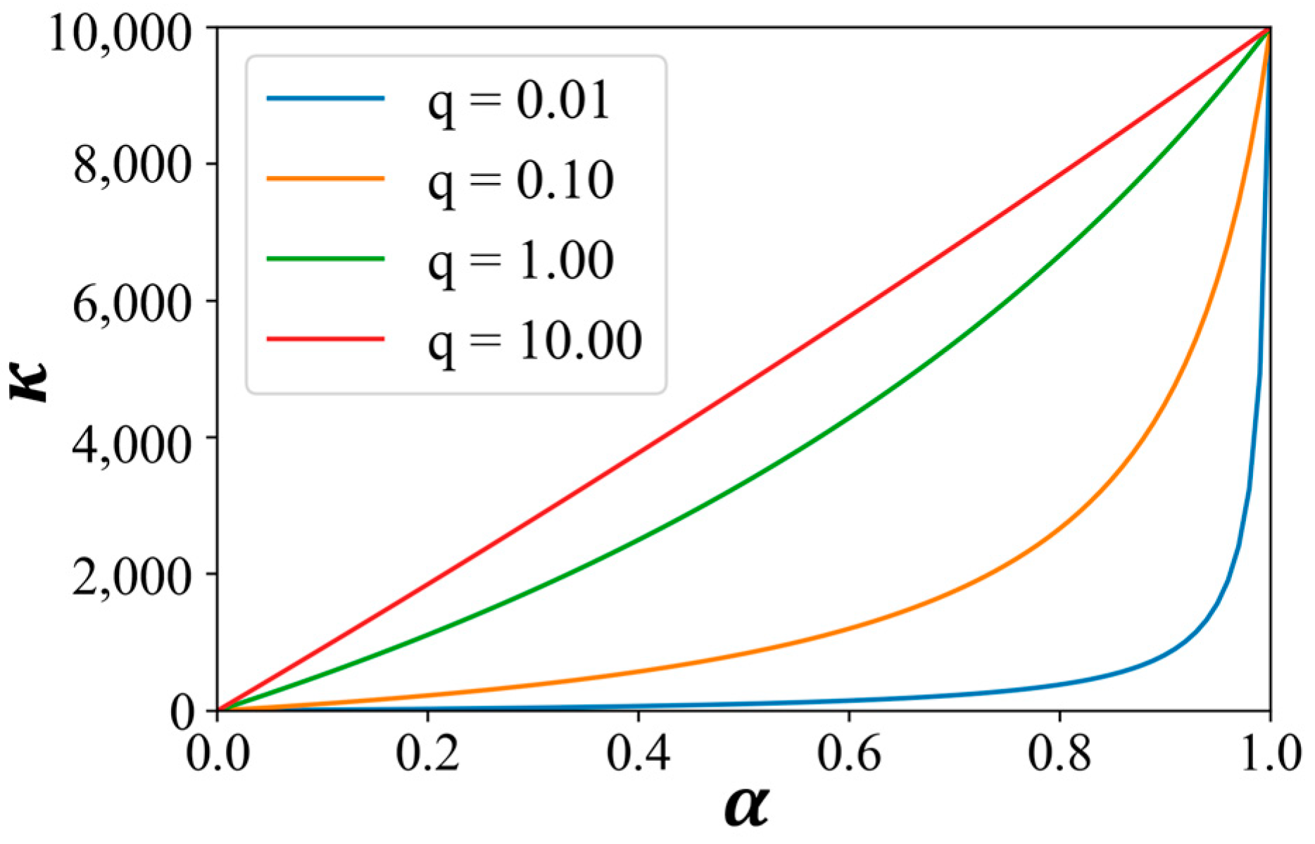
where controls the shape of , as shown in Figure 1. Borrvall et al. suggest setting a smaller () in the initial phase of TopOpt to avoid local minima and increasing it () as the optimization proceeds to obtain values of 0 or 1 s to [3]. This strategy is adopted in Section 5.3, and it works fine. However, the exact value of at different optimization stages might be fine-tuned for different values of to obtain better performance with respect to avoiding local minima.
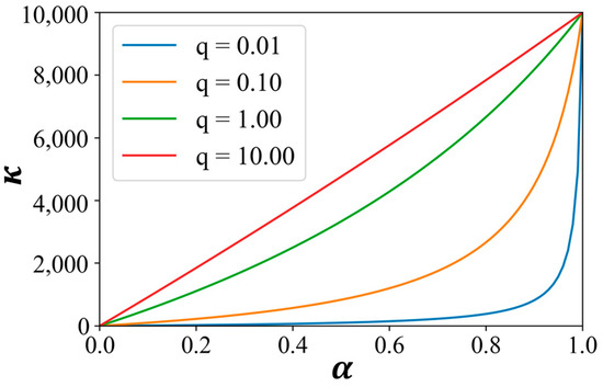
Figure 1.
’s variation with respect to α for different values of when .
Setting Equation (1) as a constraint, the mathematical formulation of TopOpt of turbulent flow based on Darcy’s source term can be written as follows:
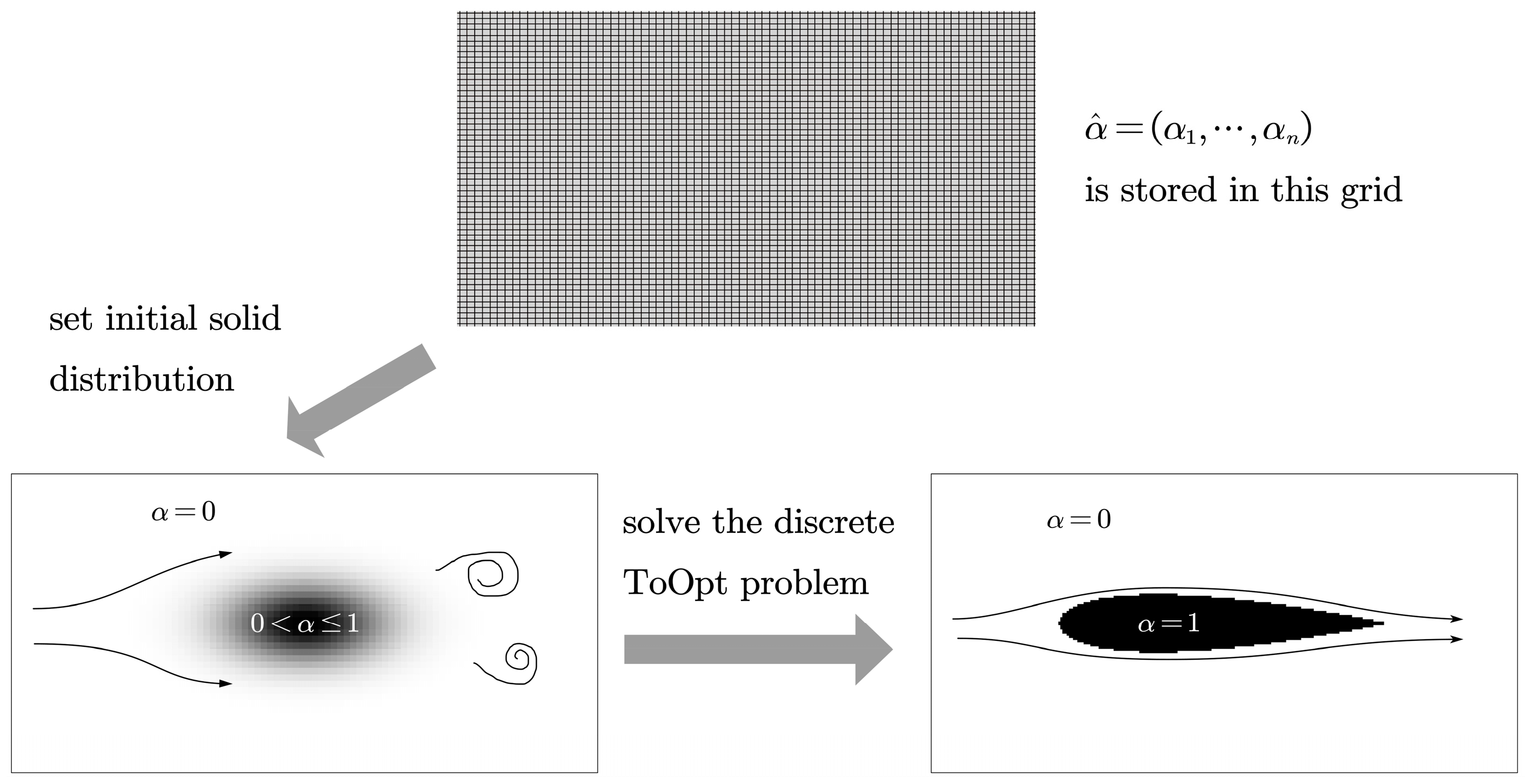
where is the objective function (functional) and is the design constraint. Since field is used to represent the solid distribution in TopOpt, an optimized solid distribution is found once the above optimization problem is solved for . In practice, the flow field is calculated by CFD, and then the objective function is evaluated. In this case, the computational domain is discretized into cells, and the functions, such as , are represented by vectors with hats () that store the respective function values in each cell. The discrete versions (the discrete equations that are solved in the CFD code) of Equations (3)–(6) can be abbreviated as follows:
Based on Equations (9) and (10), the discrete expression for TopOpt based on Darcy’s source term can be written as follows:
The process of solving the discrete TopOpt problem is illustrated in Figure 2. The functional and that generate Figure 2 can be found in Equations (24) and (26). Any vector whose elements all fall between 0 and 1 can be chosen as the initial . The gradient of the objective function and the constraint are obtained by the discrete adjoint method (which will be discussed in Section 4) during the search for the optimized distribution.
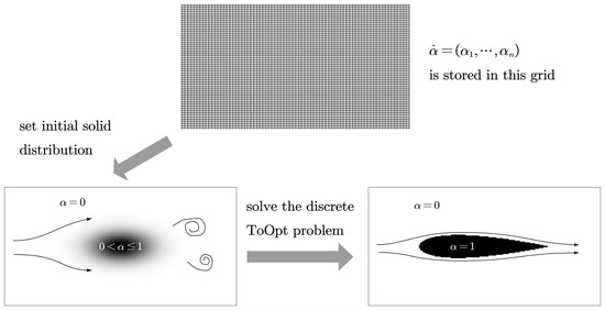
Figure 2.
The solution process of the discrete TopOpt problem.
2.2. Strategy for Setting at High Reynolds Numbers
The higher is, the more impermeable the solid modeled by Darcy’s source term. However, a large induces severe stiffness in Equation (1) (if the source term is treated explicitly) and in the adjoint equation that will be introduced later (Equation (43)), which is an undesirable feature for numerical solution [2]. Therefore, a that is as small as possible while modeling the solid with acceptable fidelity is preferred. Refs. [4,18] suggest that for a relatively low-Reynolds-number flow (), should be chosen to ensure that Darcy’s source term significantly outweighs the viscous force:
is the ratio of the magnitude of the viscous force and Darcy’s source term. In the following paragraphs, the relationship between needed to model the solid with enough accuracy and the characteristic features of the flow is investigated. If the maximum velocity in the region where is smaller than , the solid is considered to be modeled with enough accuracy. In this study, is considered to be accurate enough because of a possible direct hit of freestream on the “solid” in some optimization examples, and is studied (). Then, a strategy for setting is proposed.
Two hypotheses are needed for the derivation of :
Hypothesis 1.
When Darcy’s source term sufficiently impedes the fluid motion in the solid region (, whereis the freestream velocity), approximately satisfiy the following relations and Equation (4) (Darcy’s equation and the continuity equation) in the solid region:
Hypothesis 2.
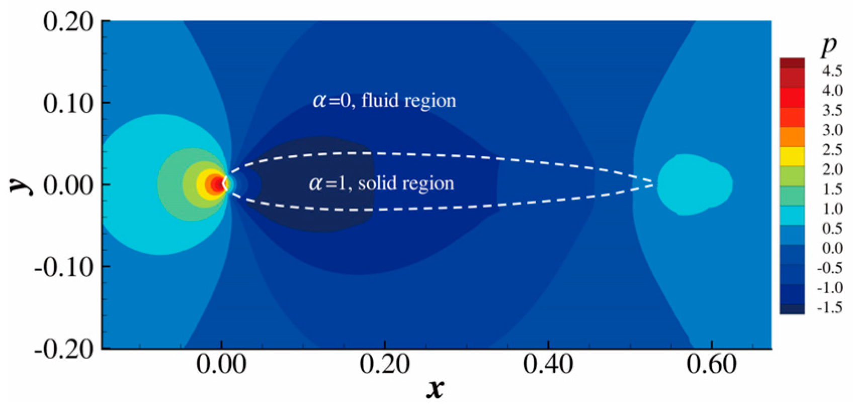
When Darcy’s source term sufficiently impedes the fluid motion in the solid region, the pressure is continuous across the solid–fluid boundary.
The above hypothesis can be tested in the following case. Darcy’s source term is used to model an airfoil. The Reynolds number based on the chord length is (consider a fully turbulent flow induced by trips at the leading edge of the airfoil), and is satisfied in the airfoil modeled by Darcy’s source term (by definition, the solid is modeled with enough accuracy in this case). For Hypothesis 1, the continuity equation holds since the flow field is obtained by solving Equation (1). Figure 3 shows that the component of the left-hand side of Darcy’s equation in Equation (12) is approximately zero in the solid region. The distribution of the component is similar. Therefore, Hypothesis 1 is demonstrated to be reasonable. Figure 4 shows that the pressure is continuous across the solid–fluid boundary, justifying Hypothesis 2.
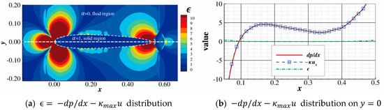
Figure 3.
Distribution of the left-hand side of the component of Darcy’s equation in an airfoil case at .

Figure 4.
Pressure distribution of the domain.
Using hypotheses A and B, it can be derived that approximately satisfies the following boundary value problem:
where is the boundary of the solid region and is the pressure distribution on the surface of the airfoil given by solving the flow field outside of the airfoil using N–S equations with a solid-wall boundary condition (without using Darcy’s source term). At a high Reynolds number, where the flow has no separation (i.e., for the airfoil, the angle of attack should be small enough to make this assumption), the viscous effect only dominates in the boundary layer and the boundary layer is very thin. Though the details of pressure distribution might be influenced by the displacement thickness, the outline and the extremum of the distribution are mainly determined by the inviscid effect. Since the approximate value of is being estimated, the viscous effect on pressure distribution is dropped here. Consequently, is only related to the freestream velocity, , the length scale of the airfoil, , and the geometry of the airfoil, . is the chord length of the airfoil, and can be viewed as the nondimensional curve defining the airfoil. The boundary value problem Equation (13) suggests that the value of in the solid region, , is only related to the shape of and the information on the boundary (). Consequently, is only related to . Using dimensional analysis and the result of the above discussion, can be written as follows:
where is a functional of , which reflects the influence of the geometry on the maximum magnitude of the pressure gradient. Hypothesis 1 indicates that the maximum velocity magnitude in the solid region satisfies the following condition:
Insert Equation (14) into Equation (15):
To ensure that , should satisfy the following:
Equation (17) suggests that the minimal needed to resist the flow is proportional to . Using the order analysis, a very important contribution by Theulings et al. [19] suggests that the order of should satisfy the following:
where is the scale of grid cells. This is similar to Equation (17), which suggests that the velocity, , and should scale linearly. The in Equation (18) comes from a very meticulous analysis of the grid-cell level in [19] that is not performed here. Based on Equation (17), the following strategy for setting is proposed:
- Set based on Equation (11) as an initial guess.
- If the initial guess is insufficient to impede the fluid motion in the solid, then is increased until the desired accuracy is obtained (the velocity in the region where is smaller than , where and is determined by the user) and the numerical solution process of the governing equations and the adjoint equations is stable.
- Suppose it is known that is enough for the TopOpt of one geometry at a low Reynolds number, , and TopOpt of the same geometry at a high Reynolds number, (), is desired. Instead of increasing the flow speed, one can keep and unchanged and adjust the fluid viscosity, (), or one can also scale and together and keep the dimensionless number unchanged. This is because, according to Equation (17), if stays the same, the accuracy of solid modeling would not change regardless of the variation in the Reynolds number. Scaling more aggressively or conservatively compared with scaling will result in suboptimal performance. Consider the ratio of the inertial term or the pressure term to Darcy’s source term. By performing magnitude analysis, the ratio can be expressed as follows:
Equation (19) indicates that if is increased more aggressively than (i.e., ), the ratio will be amplified, causing stronger stiffness, especially for the adjoint equations. On the other hand, if is increased more conservatively (i.e., ), will decrease, resulting in a downgraded blocking effect according to Equation (17).
2.3. Objective Functions and Constraints
The following objective functions and constraints are used in this paper:
- The total pressure loss, where is the computational domain and is the outer normal of the domain boundary, , is given as follows [6,20]:
The total pressure loss can measure the energy dissipation in the computational domain. However, when the grid resolution near the boundary of the computational domain is coarse, the accuracy of Equation (20) might be compromised.
- 2.
- The integration of the total dissipation rate [3,14] is as follows:
- 3.
- The approximate drag exerted on the porous medium is represented by Darcy’s source term proposed by [9]:
It can be proved mathematically [9] that Equation (24) tends to the following equation as the velocity in the region where tends to zero:
where is the combination of the viscous stress tensor and the Reynolds stress tensor, is the second-order identity tensor, is the unit vector in the direction, and is the boundary of the solid region. It can be seen that Equation (25) is the conventional formula used to calculate the drag exerted on a solid surface.
In some TopOpt examples of the following sections, the volume constraint of the solid is applied:
where is the total volume of the computational domain and is the lower bound of the volume fraction of the solid. In the optimization that uses drag (Equation (24)) as the objective, Equation (26) is used to prevent the algorithm from reducing the drag by removing the solid material. On the other hand, Equation (26) can also suppress the intermediate density () in some cases [2].
3. Turbulence Models with Modification Terms Related to Darcy’s Source Term
In this paper, two modified turbulence models that can consider the influence of Darcy’s source term are developed. To the best of the authors’ knowledge, neither of these models has been proposed in the current literature.
3.1. The Modified Launder–Sharma Model
The transport equations of the modified Launder–Sharma (LSKE) turbulence model [21] are as follows:
The terms with underbraces were proposed by Launder and Sharma and are defined as follows:
The turbulent viscosity is calculated using the following equation:
The standard model [22] necessitates the use of a wall function. The modification terms of Launder and Sharma enable the LSKE model to be integrated into the wall. Consequently, one can simply set to zero at the wall without activating the wall function when using the LSKE model.
The term underlined in the equation is proposed in the present paper and is inspired by Gil Ho Yoon’s work [15]. It is quite similar to Darcy’s source term in the N–S equation, and it compels to zero in the solid region (which means there is no turbulence in the solid region). When is compelled to zero in the solid region, is also compelled to zero, since the production term in ’s transport equation vanishes if :
Note that although and are both small in the solid region, in the solid region is still calculated by the definition in Equation (32). By assuming that the velocity is (nearly) zero in the solid region, only the second and third terms on the right-hand side remain in Equation (28). According to the magnitude analysis:
is the characteristic length of the solid. Since the above two terms are equal:
By the definition of Equation (32), . Since in the solid region, also tends to zero. Therefore, using Equation (32) to calculate in the solid region will not result in a large .
From now on, the LSKE model with Darcy’s source term modification proposed by the authors is referred to as the modified LSKE model. The modified LSKE model’s ability to describe the influence of Darcy’s source term on turbulence is tested in Section 5.
3.2. The Modified SST Model
The shear stress transport (SST) turbulence model is widely used in industry. The transport equation of the SST turbulence model [23,24] is given below:
where is defined as and is the smallest grid scale. The value of is adopted from the recommended solid-wall boundary condition for the SST model [24]. The relation between and is determined by balancing the molecular diffusion and the destruction term in Equation (37). The factor 800 was suggested by Menter [24], based on numerical experiments. Since tends to infinity near the wall, the source term was constructed to compel to in solid regions, where has a very large value. The underlined terms were originally used by Dilgen et al. in the modified Wilcox turbulence model. However, different from the Wilcox model, another fix is needed in the blending function used by the equation of the SST turbulence model. By using the blending function in ’s transport equation, the SST model switches between the standard model (activated far from the wall) and the Wilcox model (activated near the wall). This zonal formulation makes the SST model robust to use and has a good resolution near the wall. is defined as follows:
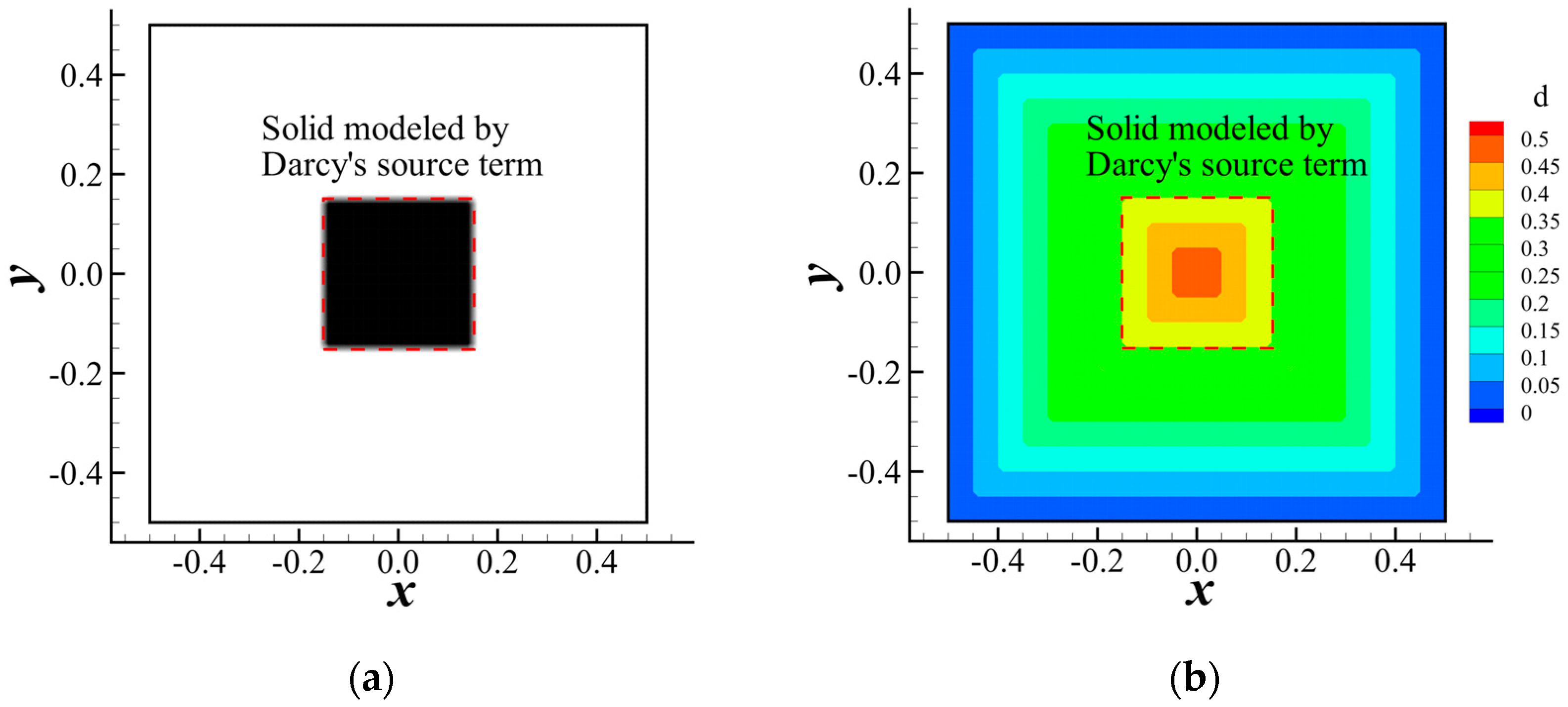
depends on the wall-distance field, , where is defined as the distance to the closest wall. is important since it directly influences the zonal formulation of the model by determining the value of . Traditional methods used to calculate have trouble recognizing the solid modeled by Darcy’s source term; hence, erroneous values around the solid region are given in TopOpt based on Darcy’s source term. Consider a square domain surrounded by walls with side length . A piece of a solid modeled by Darcy’s source term with a square shape located at the center of the domain has a side length . The true distance we expect at the edge of the solid should be zero. However, if the traditional method that only depends on real solid boundaries is used, the distance at the edge should be . This discrepancy is illustrated in Figure 5, where the wall distance is calculated by the classic mesh-wave method [25] in OpenFOAM.
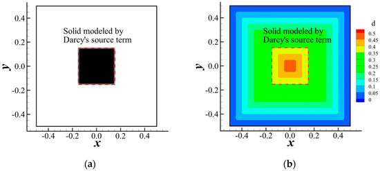
Figure 5.
The erroneous wall-distance field calculated by the mesh-wave method that does not take Darcy’s source term into account. (a) The solid modeled by Darcy’s source term. (b) The wall-distance field, , takes a nonzero value at the edge of the modeled solid.
To address this problem, a concise method based on the p-Poisson equation and normalization proposed by [26] is developed. It contains two major steps:
- Solve the p-Poisson equation with the penalization term proposed in this paper:where is larger than or equal to 2 and .
- Normalize to acquire :
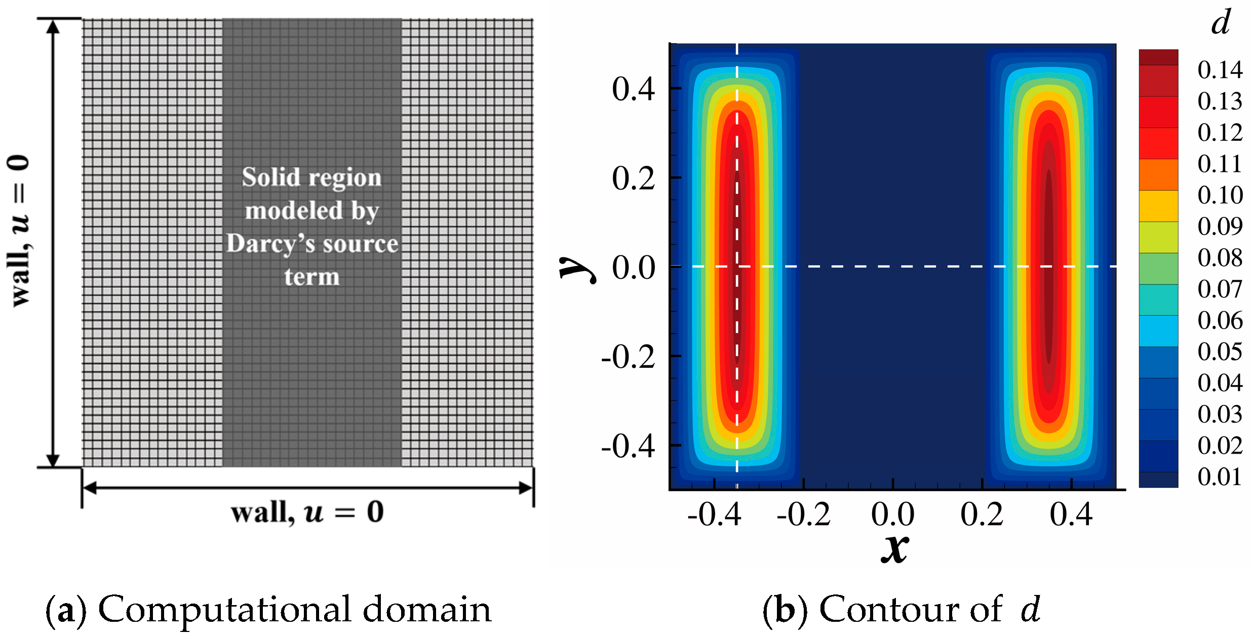
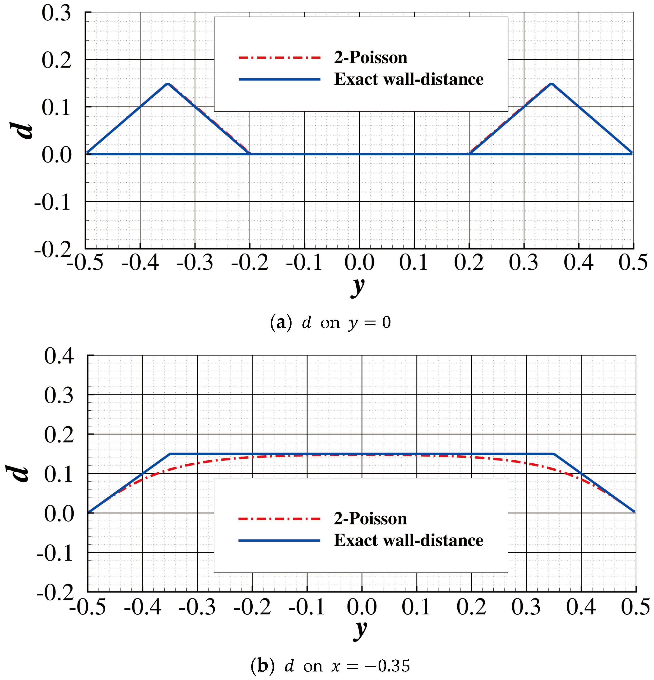
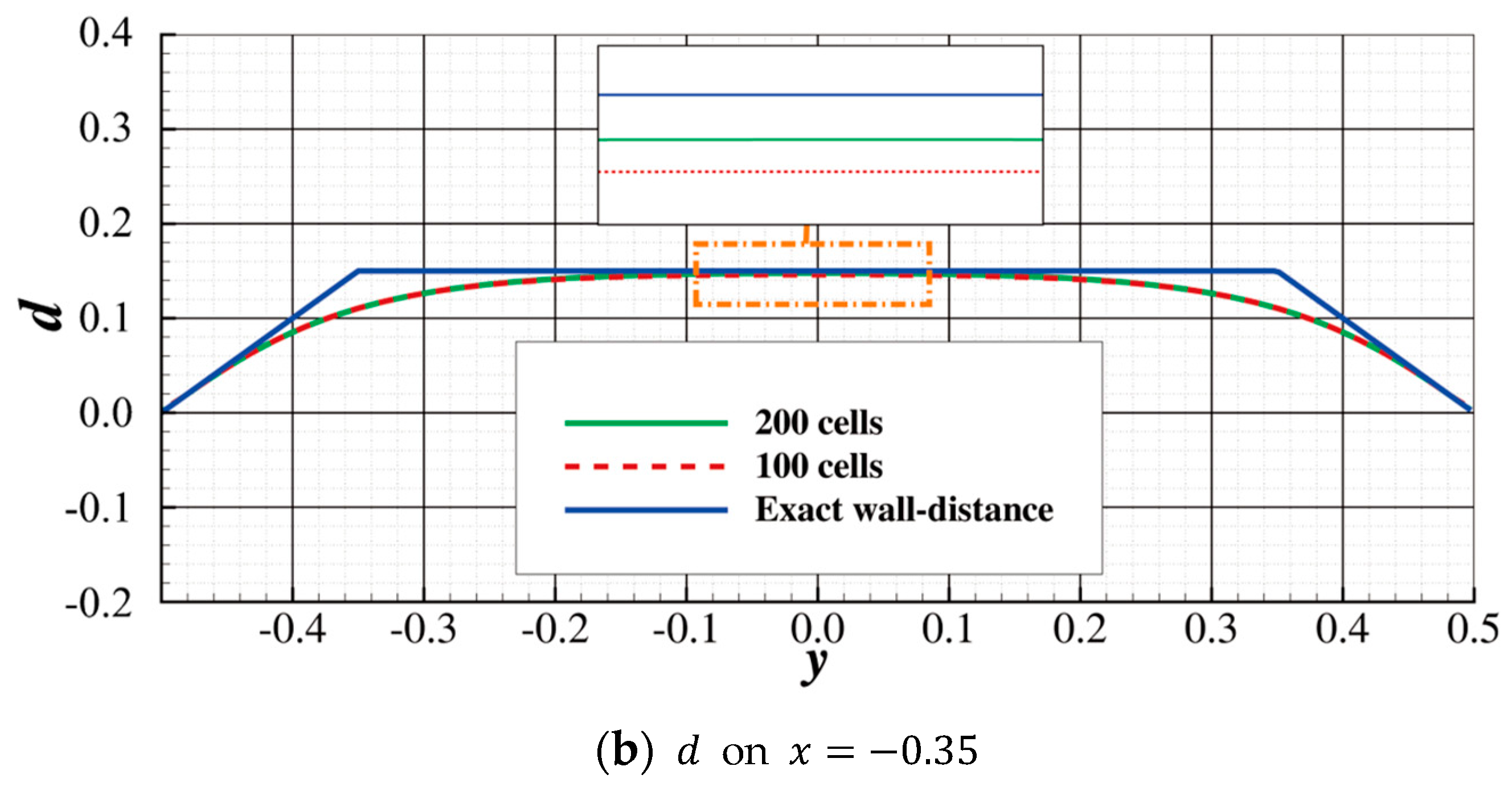
In this paper, is set to 2, and the resulting 2-Poisson equation, according to Equation (39), is linear. The accuracy of the proposed method is checked in the following test case. The wall-distance field, , is computed by the new method in the domain shown in Figure 6a. The gray area is the solid modeled by Darcy’s source term. The calculated is shown in Figure 6b. The result extracted from is plotted in Figure 7. The result given by the proposed method is almost identical to the analytical solution at . However, it deviates from the analytical solution at , where sharp corners appear in the analytical solution. Since the SST model only uses the wall-distance field to switch from the model, which is preferable within the boundary layer, to the model, the accuracy of the wall-distance field near the wall (around the boundary layer) is of the utmost importance. The wall-distance field calculated by the proposed method overlaps the analytical solution in Figure 7a,b near the wall, so the accuracy of the proposed method is sufficient. A coarser grid that uses 100 cells on each edge was also used to test the current method. The result in Figure 8 shows that the proposed scheme still performs well in this coarser grid. The validation case in Section 4.2.2 further proves the accuracy of the proposed approximate wall-distance computation method.
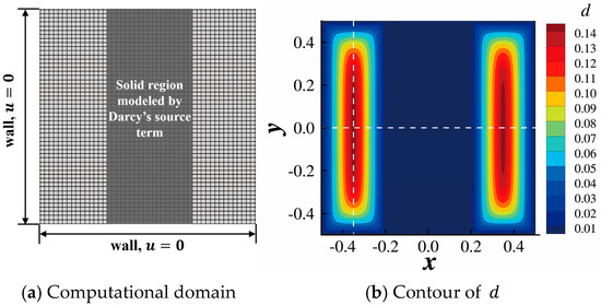
Figure 6.
Diagram of the computational domain and the result. A gird is used. For clarity, a coarsened grid is shown in (a).

Figure 7.
Comparison of the results computed by the proposed method and the analytical solution.
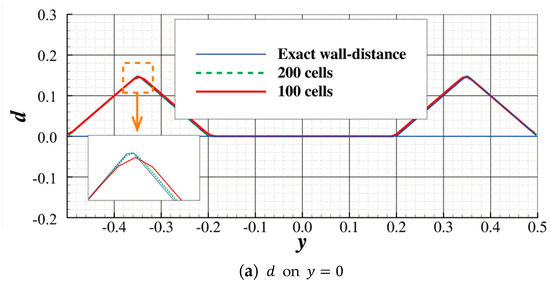
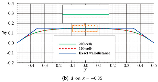
Figure 8.
Comparison of the results given by the finer grid () and the coarser grid (). The two results are almost identical.
4. Numerical Method and Validation
4.1. Numerical Method for CFD and Gradient Computation
In this study, the open-source multidisciplinary optimization program DAFoam [27,28,29] was used to solve the CFD problem and obtain the gradient of the objective function in TopOpt. The calculated objective function value and the gradient were then fed into the optimization solver pyOptSparse [30] using SNOPT’s SQP algorithm [31]. The TopOpt problem was solved by following the steps below [32,33]. The notation follows the discrete form of the TopOpt problem detailed in Section 2.1.
- Given the solid distribution , the state variable (including and turbulence variables) is calculated by solving the discrete form of the governing equations, including the momentum equation, the continuity equation, and the turbulence model equations:
Equation (41) represents the system of linear equations resulting from discretization. Take the momentum equation (2D), for example; the discretized momentum equation in the direction for cell can be written as follows:
where the variables with capital letter subscripts are variables defined for the cell center and the variables with lowercase letter subscripts are the interpolated variables for the interface, are the scale of the grid cell, is the direction velocity, and is the direction velocity. To avoid a checker-board pressure distribution, momentum interpolation might be introduced to obtain [34]. Readers who are interested in the detailed and full definition of are referred to the article devoted to the discrete adjoint method [27].
After solving Equation (41), the values of the objective function and the constraint are calculated.
- 2.
- The Jacobians , , and are computed using automatic differentiation (AD) [35,36], which is designed to evaluate the derivative of any function specified by a computer program. The core idea of AD is that, for any program, no matter how complicated it is, its output is always defined by a series of elementary operations for which the derivative is easy to compute. Due to this characteristic, the chain rule can be applied repeatedly to these operations to evaluate the derivative of the final output of the program to the inputs. By using this strategy, AD can compute the derivative of any computer program accurately to machine precision.
- 3.
- The adjoint vector is calculated by solving the linear equations (adjoint equations):
- 4.
- The gradients of the objective function and the constraint are computed:
- 5.
- and are fed into pyOptSparse, and the SQP algorithm is used to update the solid distribution, .
Steps 1 to 5 are repeated until the convergence criteria specified for pyOptSparse are achieved. The default criteria of pyOptSparse are used here. When the major optimality tolerance drops to , the optimization loop ends. The optimality tolerance measures how optimal a solution is based on the current gradient information. The clear definition of major optimality is beyond the scope of the paper, and readers are referred to [37]. Note that the magnitude of Darcy’s source term, , always appears on the diagonal of , which will increase the condition number of the matrix (the “stiffness” of the equations). Consequently, a smaller is more favorable for the numerical solution of Equation (43).
4.2. Validation of the CFD Solver
In this study, DAFoam’s DASimpleFoam solver (which is identical to the well-known simpleFoam solver of OpenFOAM) was used to solve the CFD problem. Two cases that are similar to the optimization examples in the next section will be calculated here to validate the solver. In all validation cases here, Darcy’s source term is not included because we only want to focus on the numerical method in this section. The accuracy of the proposed wall-distance calculation method when Darcy’s source term is involved is illustrated in Section 3.2. The accuracy of the modified LSKE model when the solid is modeled by Darcy’s source term in the mesh that can resolve the wall turbulence will be discussed later in Section 5.1.
4.2.1. NACA0012, LSKE Model
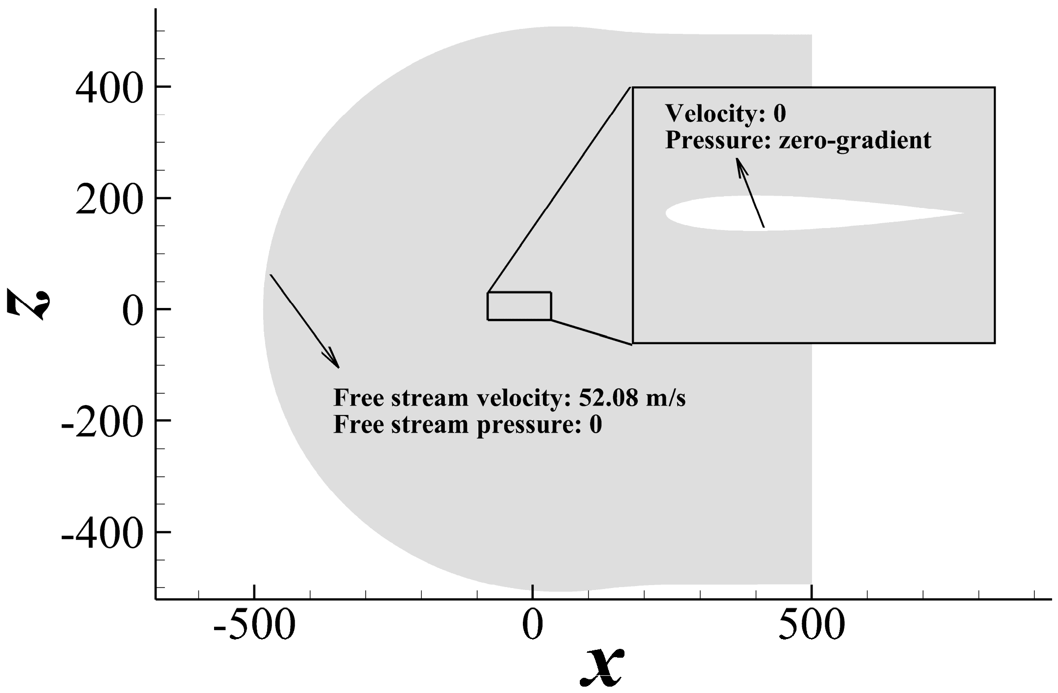
In this subsection, NASA’s NACA0012 validation case [38] is calculated using the LSKE model. The LSKE model will be used in the low-drag profile optimization later in Section 5.1, which is similar to this validation case. The family II grid provided by NASA [39] with cells is used to carry out the computation. The Reynolds number based on airfoil chord length is , and the angle of attack () is set to . The computational domain and the boundary conditions are shown in Figure 9. The turbulent variables, are set to in the freestream and are set to 0 on the airfoil surface.

Figure 9.
The computational domain and the boundary conditions.
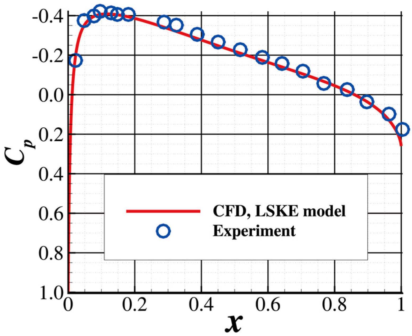
A comparison of the experimental distribution [40] and the computed result is shown in Figure 10. The result given by the current solver agrees well with the experimental data. The computed drag coefficient is compared with the tripped (corresponding to a fully turbulent boundary layer) experimental data obtained by Ladson [41]. The result is shown in Table 1. It can be seen that the relative error between the experimental data and the current result is 2.2%, suggesting that the precision of the viscous force is also acceptable.
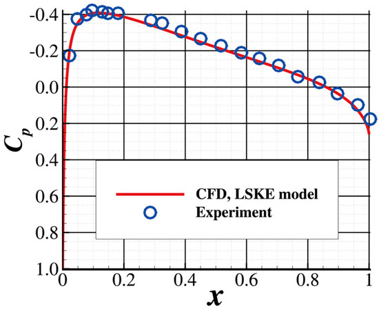
Figure 10.
distribution at .

Table 1.
Drag coefficient () comparison.
4.2.2. Backward-Facing Step, SST Model + 2-Poisson Wall-Distance Approximation Method
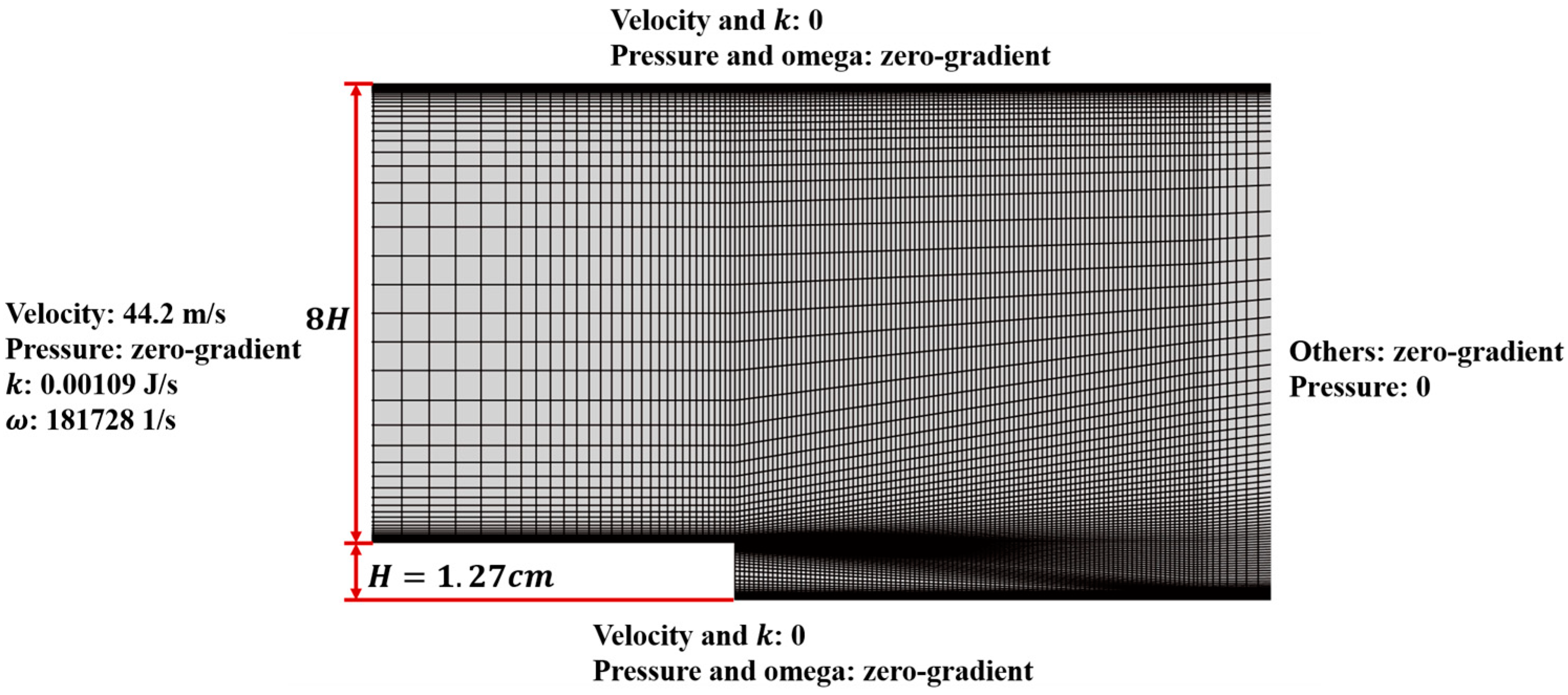
NASA’s 2D backward-facing step validation case [42] is solved by DASimpleFoam using the SST model, with the wall distance computed by the 2-Poisson equation introduced in Section 3.2. Optimization examples with a similar geometry can be found in Section 5.2. The grid generated by OpenFOAM’s blockMesh utility [43] is shown in Figure 11. The height of the step and the channel are marked in the figure. Note that the total length of the computational domain in the streamwise direction is (the distance between the inlet and the step + the distance between the step and the outlet), and only a part of the mesh is shown in Figure 11. The boundary conditions are also shown in Figure 11. The Reynolds number based on the height of the step is . Equations (39) and (40) are used to compute the wall-distance field needed by the SST model.
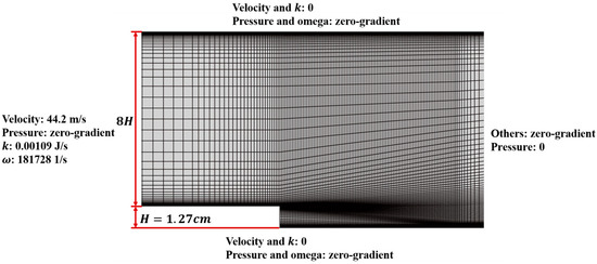
Figure 11.
The computational grid (only part of it is shown) with 20,540 cells.
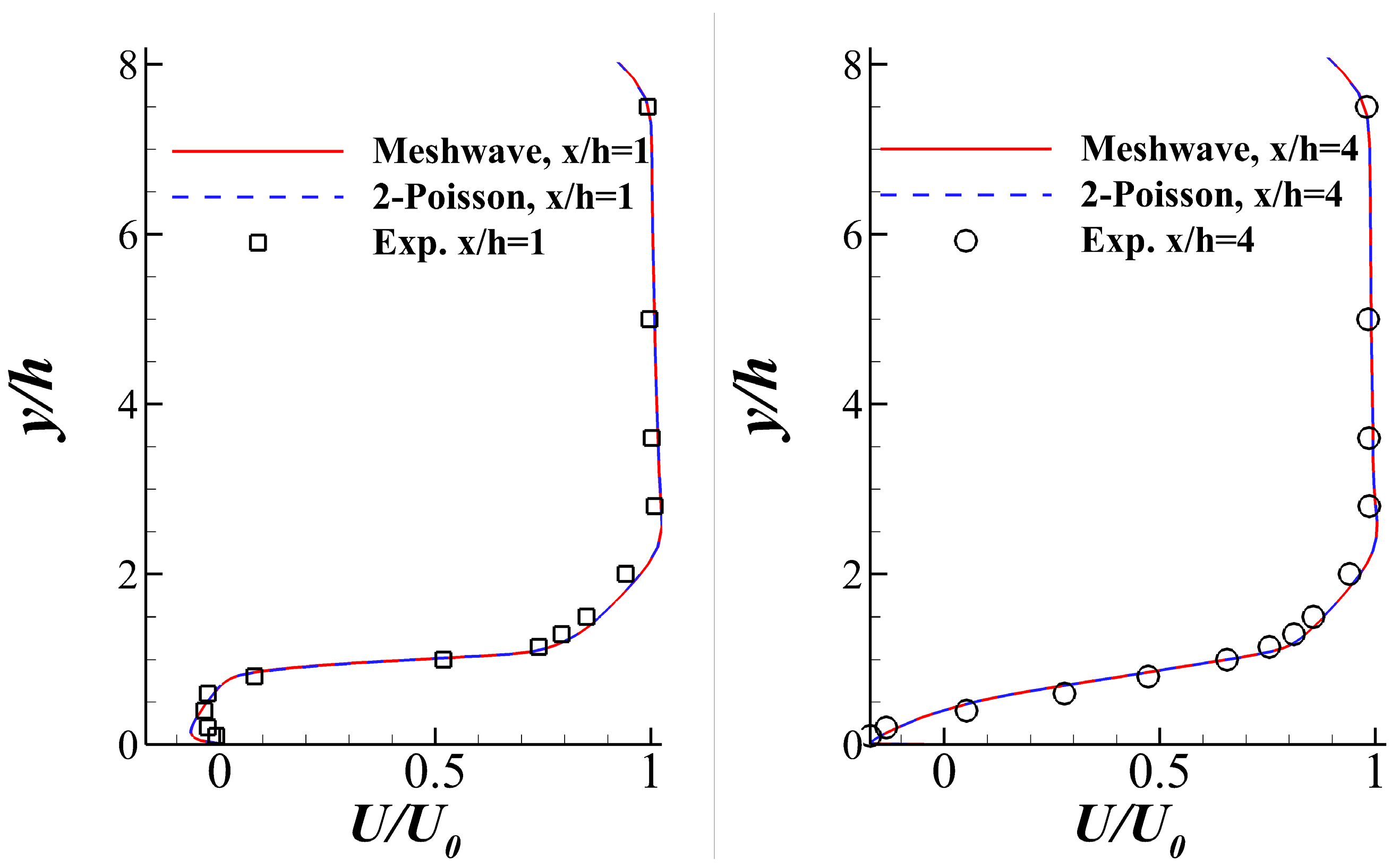
The computed velocity profiles at and downstream of the step are shown in Figure 12. Experimental data [44] and the result given by the SST model + the mesh-wave method [45] (the default wall-distance calculation method with high accuracy provided by OpenFOAM) are also plotted for comparison. The meaning of each line style is documented in Table 2 for clarity. Figure 12 shows that the velocity profiles obtained by the mesh-wave and 2-Poisson equations are almost identical, suggesting that the accuracy of the proposed wall-distance calculation method in Section 3.2 is acceptable. On the other hand, the results of CFD agree well with the experimental data. The location of the reattachment point is shown in Table 3. The comparison suggests that the precision of the reattachment point of the current solver is also satisfactory.
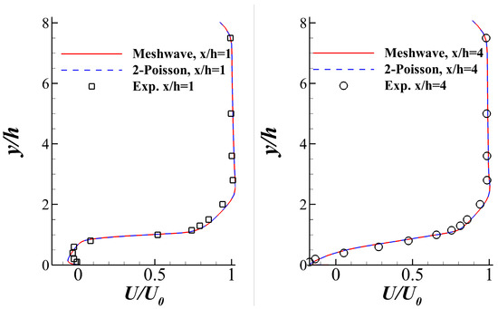
Figure 12.
Velocity profile comparison at and .
Table 2.
The meaning of each line style in Figure 12.
Table 3.
The comparison of the reattachment point.
5. TopOpt Examples
In this section, some TopOpt examples related to aerodynamic design are presented. Whenever the flow is assumed to be turbulent, the modified turbulence model developed in Section 3 is implemented. The ability of the modified models to depict the interaction between Darcy’s source term and the turbulence is also tested in some examples.
5.1. Optimization of the Low-Drag Profile
The TopOpt of the low-drag profile in the external flow was first studied by Borrvall et al. [2], assuming that (Stokes flow). It was revisited in [9], and the solution at various Reynolds numbers for laminar flow was studied. In this example, we extend the TopOpt of the low-drag profile to turbulent flow by using the modified LSKE turbulence model. In this subsection, the approximate drag (Equation (24)) is chosen as the objective function:
and the volume fraction of the solid (Equation (26)) is constrained to be no less than :
5.1.1. Re = 600, Laminar Flow
The initial solid distribution is set according to the expression below:
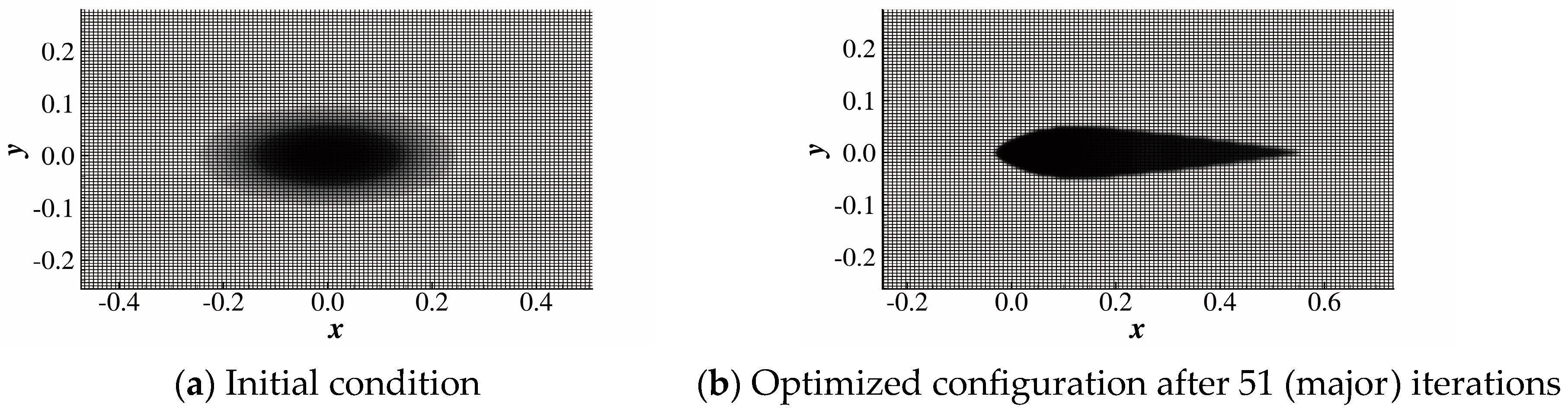
where . Rather than setting , where and elsewhere, this initial condition can avoid vortex shedding induced by the shear layer instability while still concentrating the solid in the ellipse. The initial condition and the computational grid are visualized in Figure 13a. The grid is composed of a rectangle. After 100 minor iterations (51 major iterations) in pyOptSparse, a profile with a blunt head and sharp tail is achieved, which is quite similar to an airfoil. After the optimization process, the nondimensional approximate drag is reduced from 0.17 to 0.10. The nondimensional approximate drag, , is defined as follows:
where is the freestream velocity and is computed using Equation (45). The reduction ratio is approximately 41%, showing the effectiveness of the present optimization.
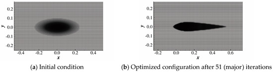
Figure 13.
Evolution of the solid distribution. Optimization is conducted on a grid composed of rectangles.
The relative thickness of the current result is compared with the results given in [9]. In the present study, the Reynolds number is calculated based on the chord length of the profile. However, in [9], the Reynolds number is based on the square root of the solid area, . The Reynolds number based on of the current result is . The results of the optimized configuration at and are given in [9], as shown in the first two columns in Table 4. The thickness of the current result lies between the results of [9]. This is reasonable, since the Reynolds number of the current result also lies between the Reynolds number investigated in [9]. Due to the lack of grid information in [9], the same grid cannot be used here, so the comparison below is rather qualitative. The comparison shows qualitatively that, for laminar flow, the higher the Reynolds number, the thinner the optimized profile.
Table 4.
Relative thickness comparison. The results of the first two columns are drawn from [9].
5.1.2. Turbulent Flow
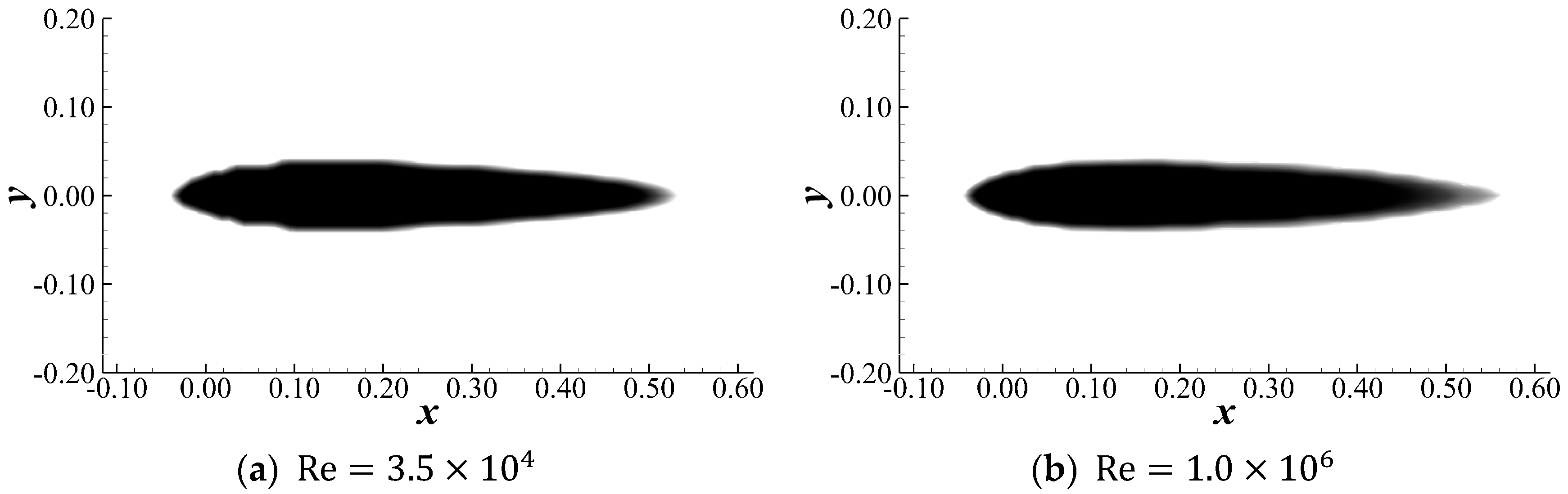
The low-drag profile is obtained at and . The flow is assumed to be fully turbulent. The parameters used at different Reynolds numbers are listed in Table 5. at was chosen according to Strategy 1 in Section 2.2 and was found to be sufficient to impede the fluid flow in the solid region (, where , except for a region around the leading edge directly hit by the freestream where . The scale of this region is less than 1% of the chord length, so it is still included in the solid region to make the optimized configuration smooth). At , are kept unchanged and is decreased to acquire a higher Reynolds number according to strategy 3 in Section 2.2. This parameter setting avoids a significant increase in the equation stiffness induced by a larger . The intermediate solid distribution during the optimization process at is used as the initial condition.
Table 5.
Parameters at different Reynolds numbers.
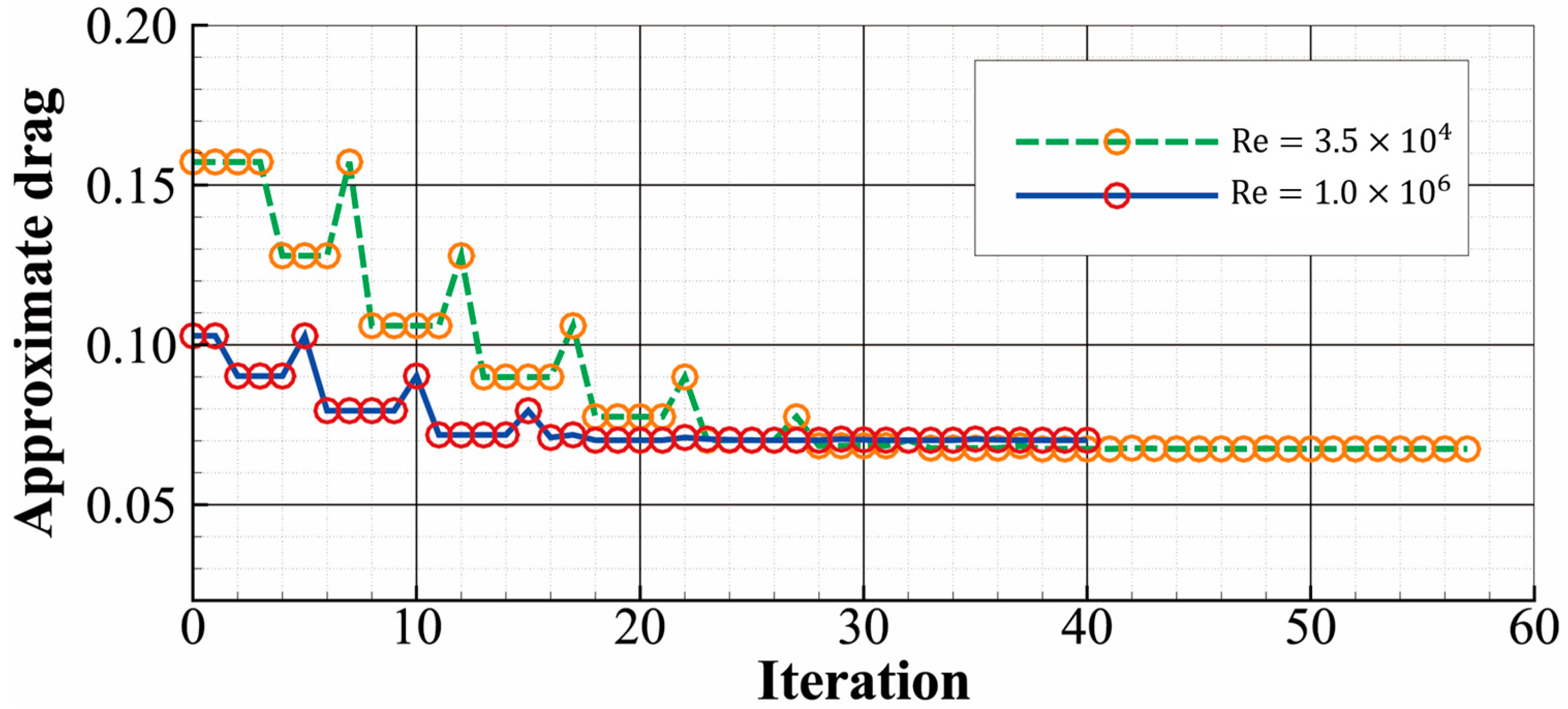
The optimized configurations are presented in Figure 14. Both configurations have a blunt nose, a sharp tail, and a smaller thickness compared with their laminar counterparts. As shown in Figure 15, the nondimensional, approximate drag decreases by 56% and 30% at and , respectively, indicating the effectiveness of the optimization process.
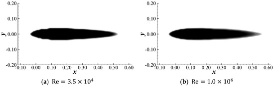
Figure 14.
Optimized low-drag profile in turbulent flow.
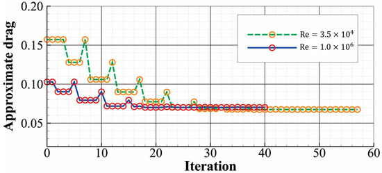
Figure 15.
Convergence history of the nondimensional, approximate drag. The value in Equation (8) is set to 0.005 here.
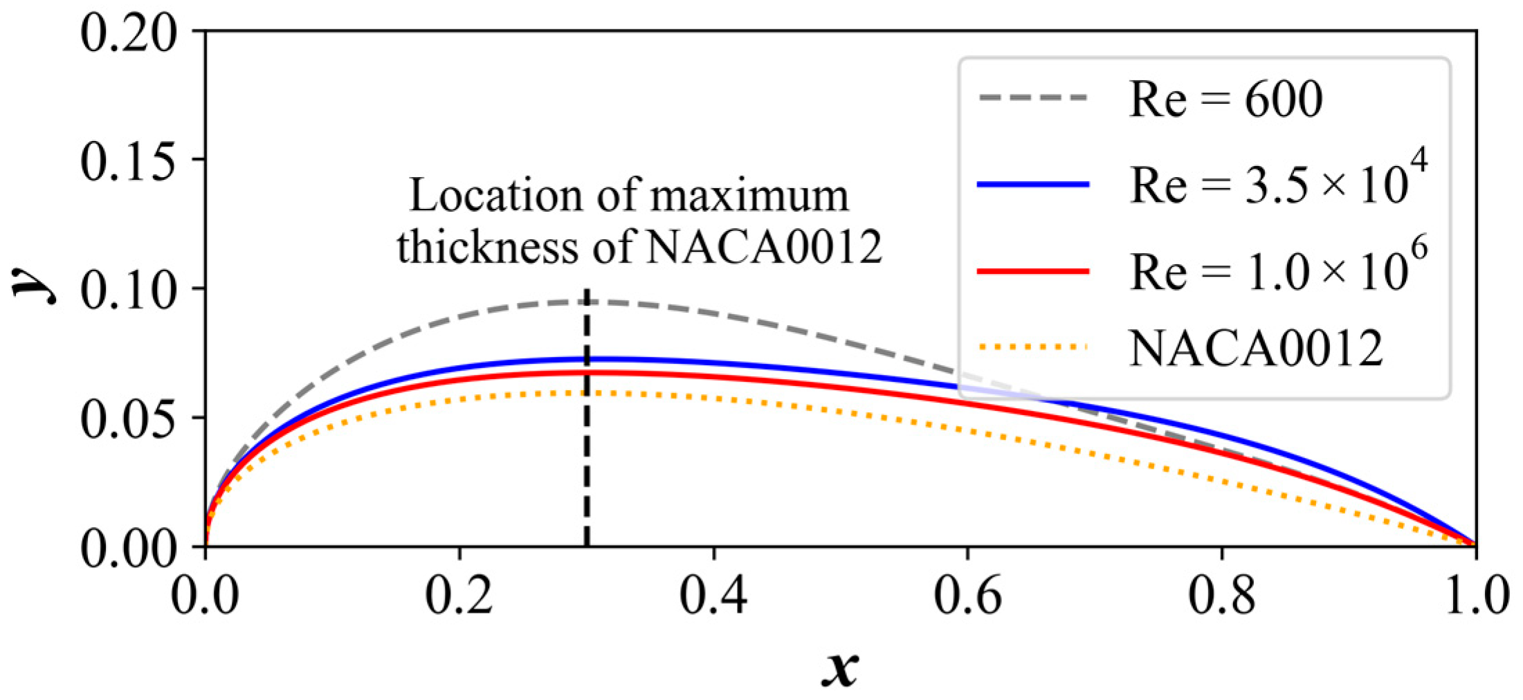
The class-shape transformation (CST) [46] method was then applied to extract a smooth profile from the optimized configuration obtained by TopOpt, as shown in Figure 16. For the turbulent case, the optimized profiles at different Reynolds numbers are similar. This is partly caused by treating the boundary layer as fully turbulent in both cases, while the low-Reynolds-number case might involve the transition effect. The optimized profile at is slightly thinner than its counterpart at . The optimized profile in laminar flow () is quite different from the ones in turbulent flow, having a larger relative thickness. Both turbulent profiles are slightly thicker than the NACA0012 airfoil, but the location of the maximum thickness is quite similar (at approximately ). The resemblance between the smoothed profile and the existing widely used airfoil indicates that the current result is physically reasonable.
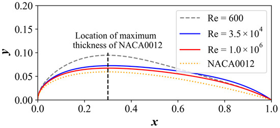
Figure 16.
Smoothed optimized profile.
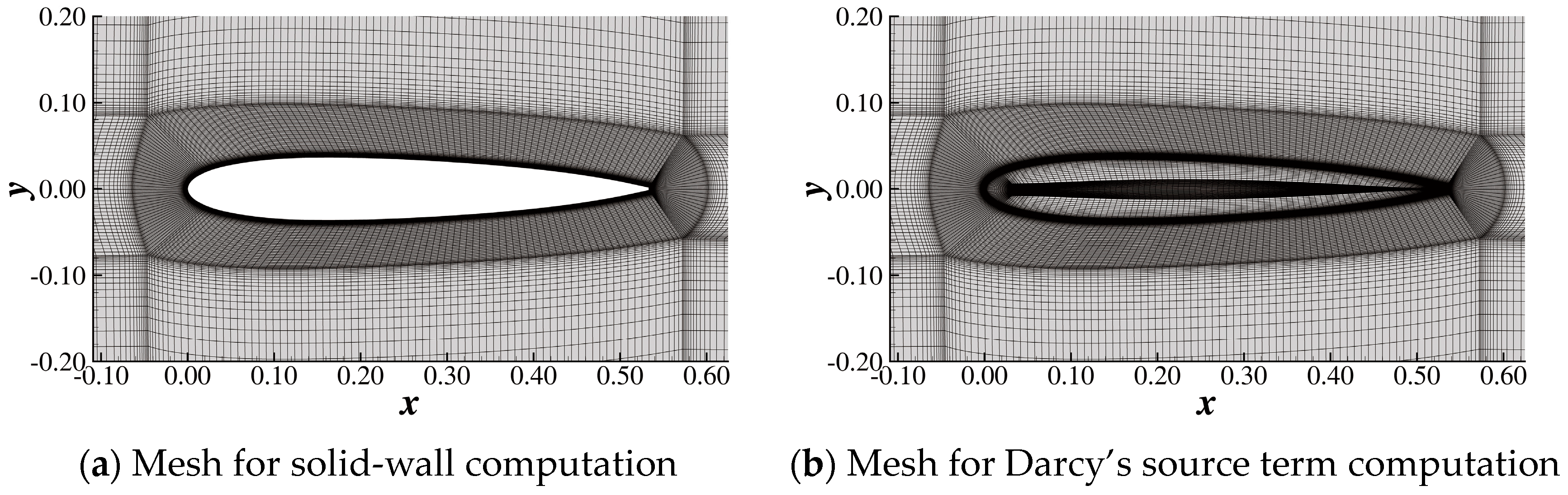
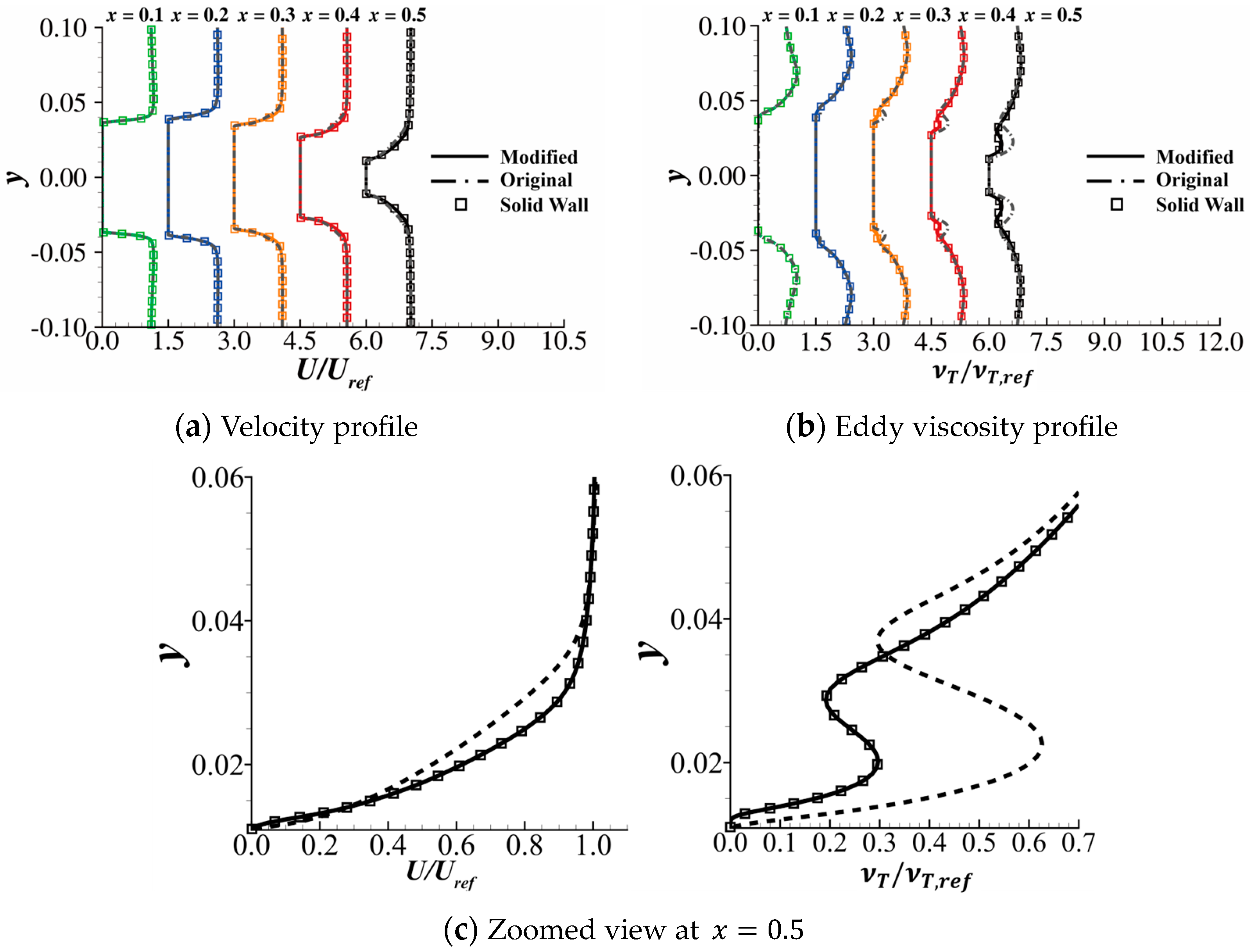
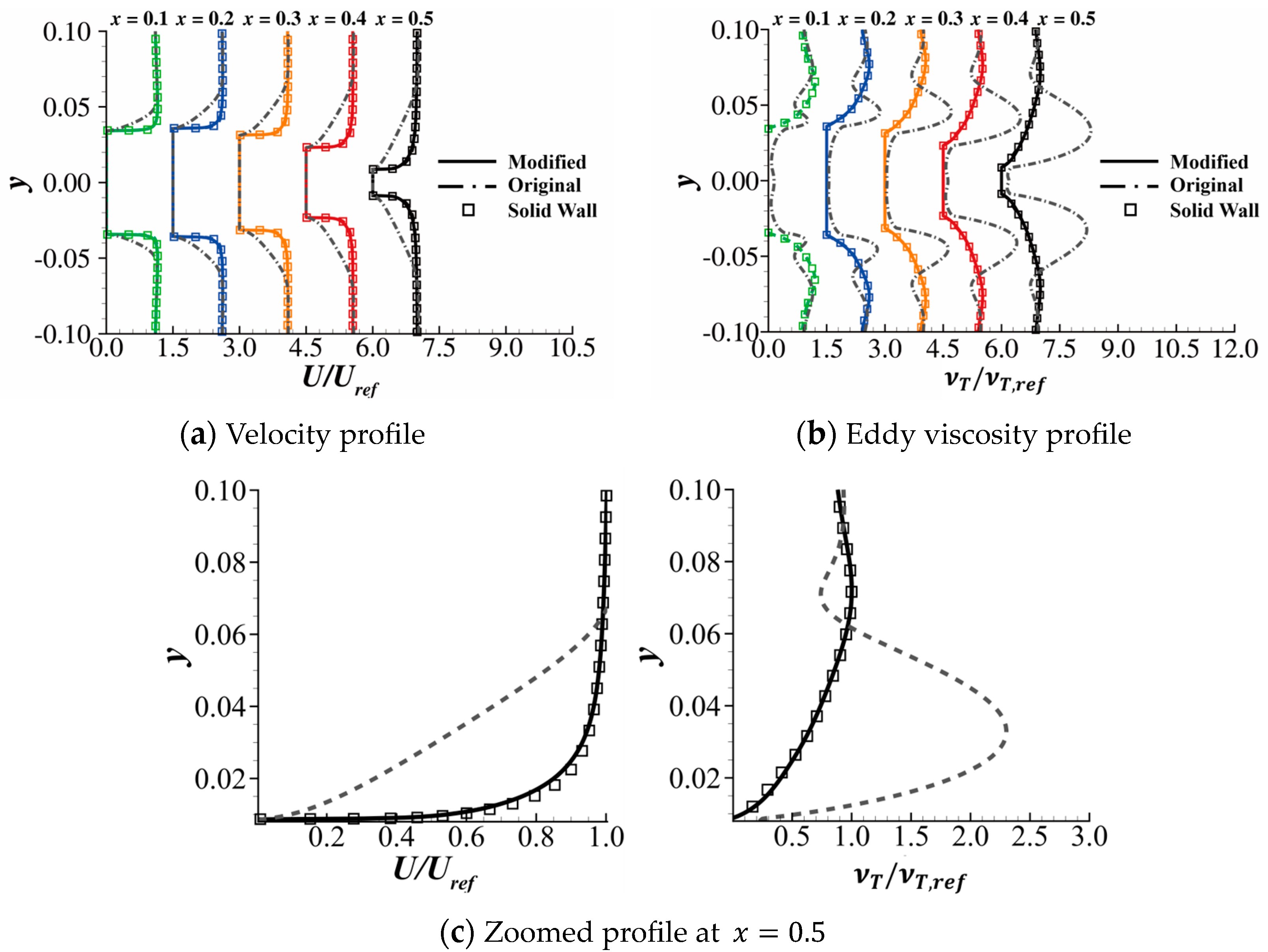
The flow field around the smoothed profile was obtained by the modified LSKE model with Darcy’s source term to model the solid and the original LSKE model with a traditional solid-wall boundary condition. Two kinds of body-fitted meshes were generated for solid-wall computation and Darcy’s source term computation. As shown in Figure 17, the only difference between the two meshes is that the solid domain is also covered by a grid in the mesh for Darcy’s source term computation. The velocity profile and the eddy viscosity profile are plotted in Figure 18 and Figure 19. For clarity, the calculation method used for each line is documented in Table 6. The profiles are almost identical. This result indicates that the modified LSKE model can reflect the influence of Darcy’s source term on turbulence with enough accuracy, even when the Reynolds number is as high as .
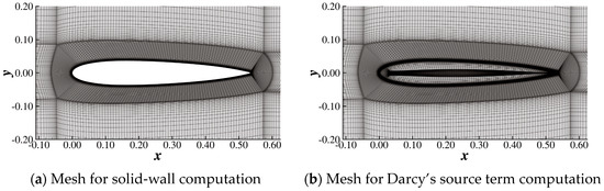
Figure 17.
Body-fitted mesh generated around the smoothed profile obtained at . The corresponding mesh for is quite similar.
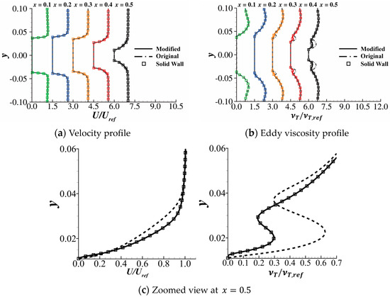
Figure 18.
Profile comparisons at ; the symbols are the results given by the original LSKE model with solid-wall boundary conditions. For every 0.1 increase in x, the result is shifted to the right by 1.5 units.
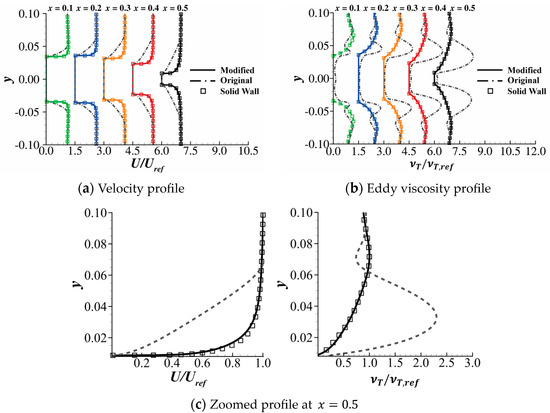
Figure 19.
Profile comparison at . The symbols are the results given by the original LSKE model with solid-wall boundary conditions. For every 0.1 increase in x, the result is shifted to the right by 1.5 units.
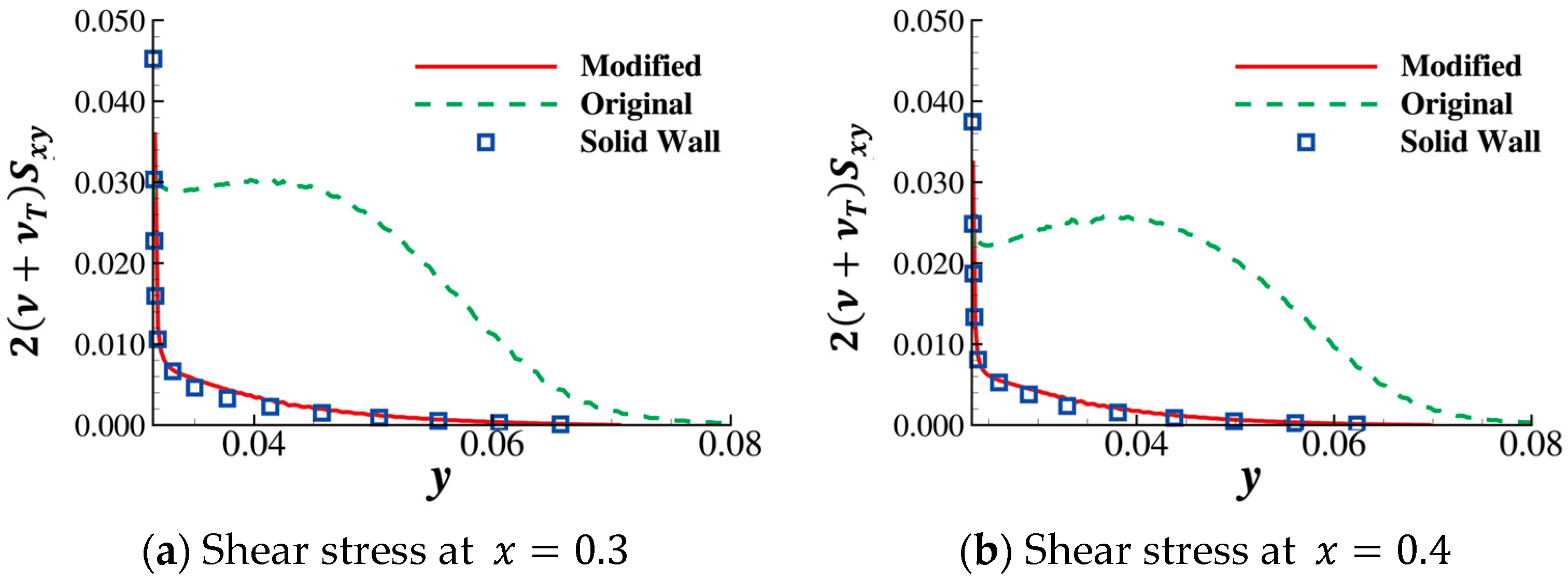
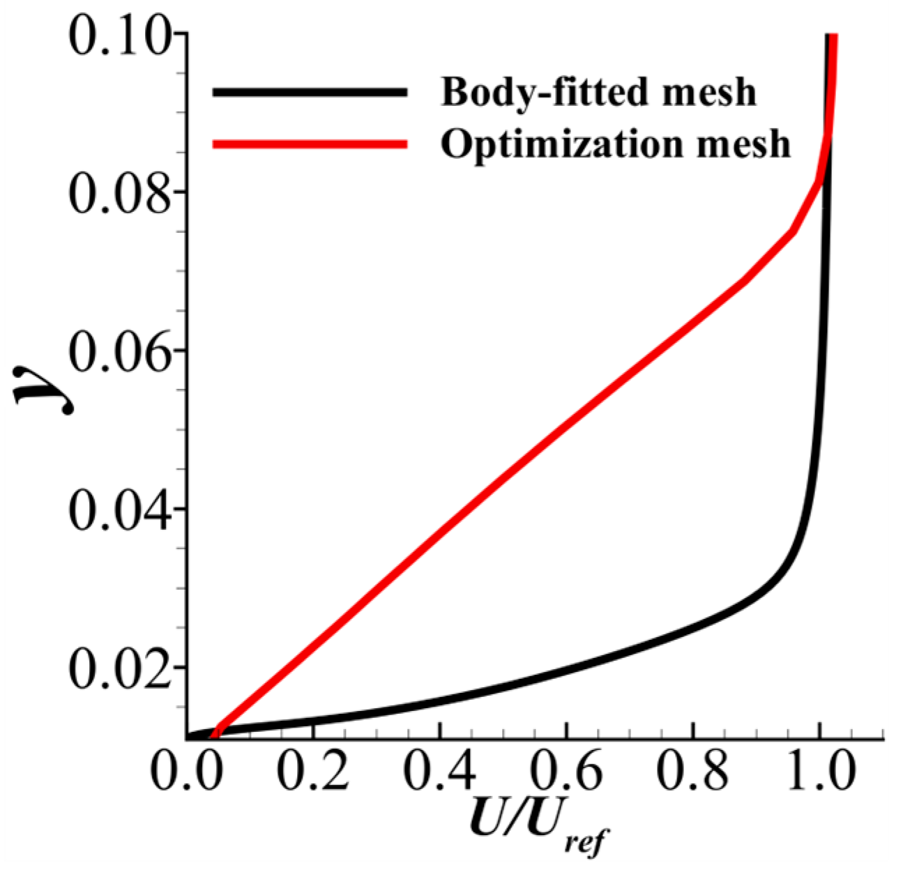
The necessity of the fix related to Darcy’s source term in the modified LSKE model can be demonstrated as follows. Figure 18b shows that the eddy viscosity profile calculated without the fix deviates from the solid-wall distribution near the wall. A zoomed view at is shown in Figure 18c, showing the discrepancy more clearly. This deviation is much more severe at and causes a large error in the velocity profile indicated by Figure 19. The deviation induced by the LSKE model without the fix can also be seen in the contours of the flow variables. The shear stress profiles at along are plotted in Figure 20. The result shows that the profile computed by the corrected LSKE model agrees well with the solid-wall solution and is a significant improvement compared with the original model. However, unlike the solid-wall boundary condition, the velocity is not stipulated to be zero at the solid–fluid interface when Darcy’s source term is used to model the solid. Consequently, the shear stress immediately adjacent to the wall is not quite accurate. Figure 21 compares the flow field at computed by three methods using the contour of the field variables, which might be a more intuitive way to show the results in Figure 19 and Figure 20: solid-wall computation (baseline), Darcy’s source term computation with the modified LSKE model, and Darcy’s source term computation with the original LSKE model. The velocity field and the turbulent kinetic field calculated by the modified LKSE model agree well with the baseline. However, the boundary layer obtained by Darcy’s source term with the original LSKE model is significantly thicker than the baseline, which is nonphysical at . The accuracy of the modified LSKE model degrades on the mesh used for the optimization, as shown in Figure 22. This is because, during the optimization, the grid points are distributed uniformly since we do not know from where the solid will emerge. Additionally, the cells are relatively large in the optimization, making it hard to directly resolve the boundary layer caused by the solid. Consequently, there are still problems in the resolution of turbulence during the TopOpt process. However, as shown in Figure 18, Figure 19, Figure 20 and Figure 21, the modified LSKE model gives an asymptotically correct prediction of turbulence when the grid resolution is good enough near the wall. The asymptotically (as the grid becomes denser) correct behavior is the basis for true turbulence resolution in TopOpt, and the modified LSKE model proposed here can achieve it. To make the turbulence prediction more accurate, future work might focus on developing wall functions considering Darcy’s source term.
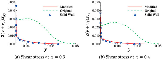
Figure 20.
The shear stress () comparison at along the wall’s normal direction.
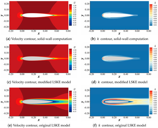
Figure 21.
Comparisons of the three computations at (right column: velocity contour; left column: turbulent kinetic energy; region where or is cut off).

Figure 22.
The discrepancy between the results for the body-fitted mesh and the optimization mesh, obtained using the optimized profile at , .
Considering the above observation, in general, the modification related to Darcy’s source term in the corrected LSKE model proposed in this paper can lead to improved results.
5.2. Rearward-Facing Step
In this study, the TopOpt of the classic rearward-facing step [47] is considered using the modified SST turbulence model. The objective function in this case is the total pressure loss, (see Equation (20)):
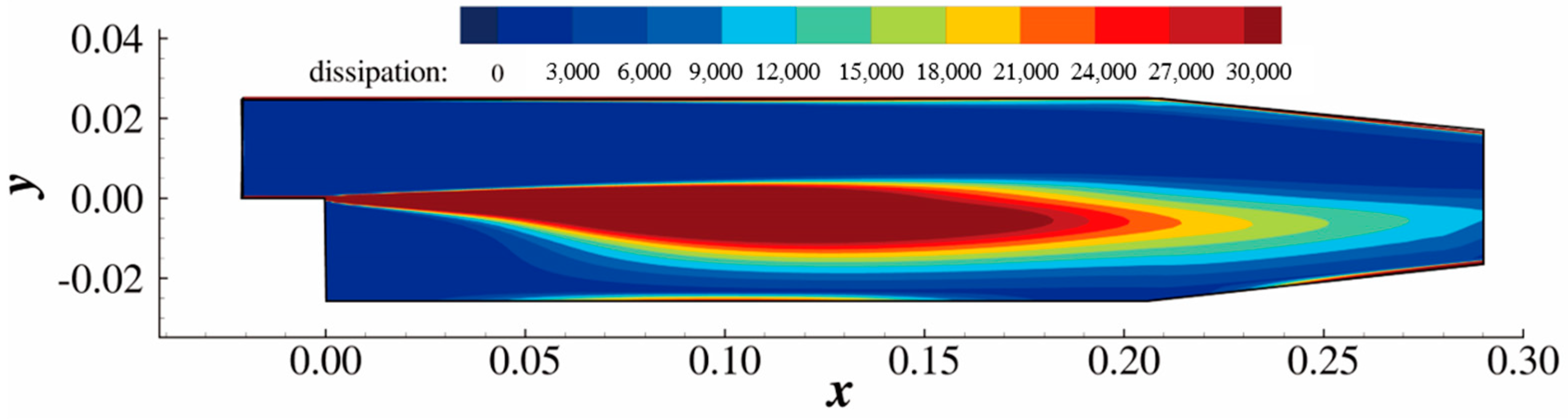
The total pressure loss is a measure of energy dissipation. No constraints are added in this case. In other words, the algorithm will explore all configurations possible to decrease the dissipated energy in the domain. is set to based on Strategy 1 in Section 2.2. The Reynolds number based on the step height is 70,000. A large separation bubble is observed behind the step, as shown in Figure 23. The viscous dissipation rate (Equation (22)) distribution is plotted in Figure 24.
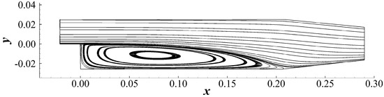
Figure 23.
Initial condition and flow field.
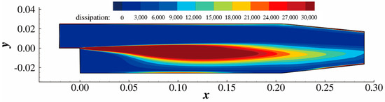
Figure 24.
Viscous dissipation rate distribution.
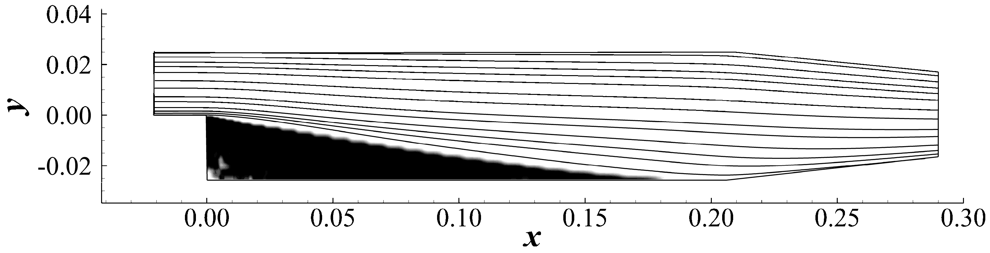
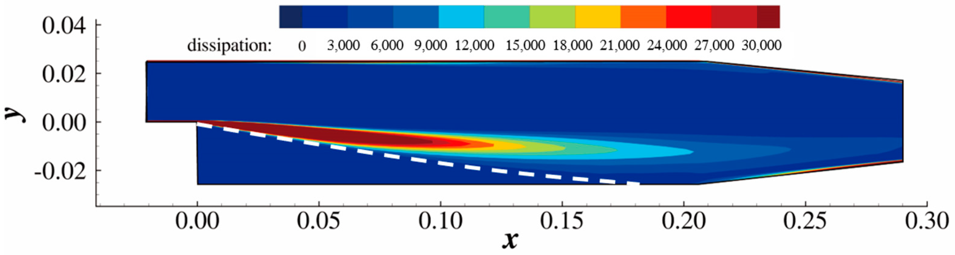
The optimization converged after 19 major iterations and the convergence criteria were satisfied, as shown in Figure 25. The number of iterations here is slightly low since the TopOpt problem is relatively easy to solve. The reduction in the total pressure loss is shown to be 55%. In the optimized configuration, the separation bubble is eliminated by the solid distributed behind the step, as shown in Figure 26. Note that a geometry closer to a plane channel might result in a higher bulk velocity and thus a higher friction. So, it is reasonable to have an optimized solution, as shown in Figure 26. The viscous dissipation rate is effectively suppressed in the optimized configuration compared with Figure 24, as shown in Figure 27.
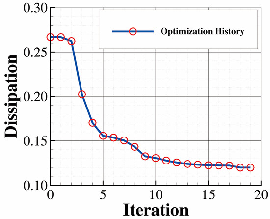
Figure 25.
Convergence history of , major iteration.

Figure 26.
Optimized configuration.
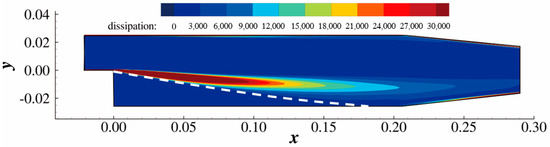
Figure 27.
The viscous dissipation rate is largely reduced in the optimized configuration.
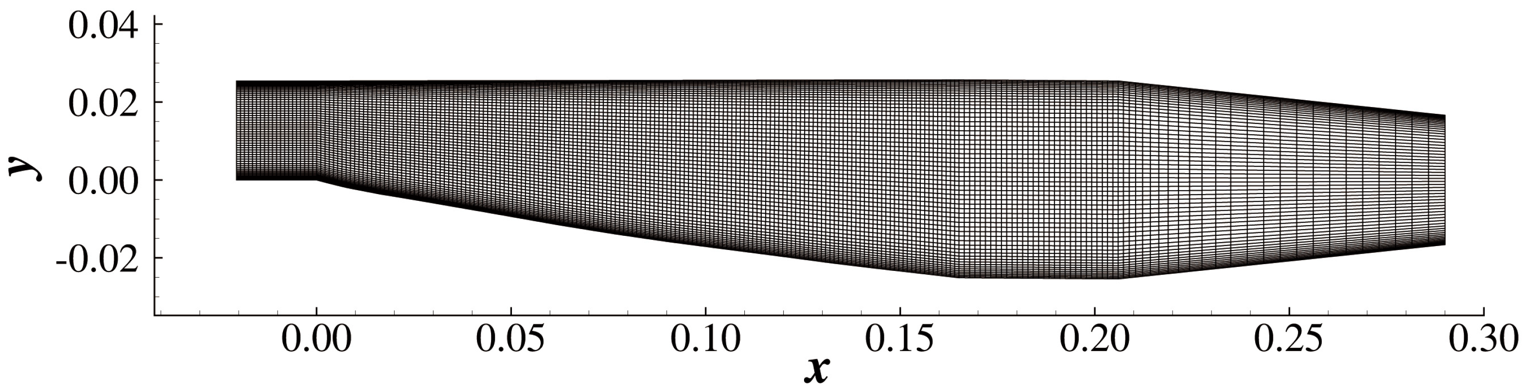
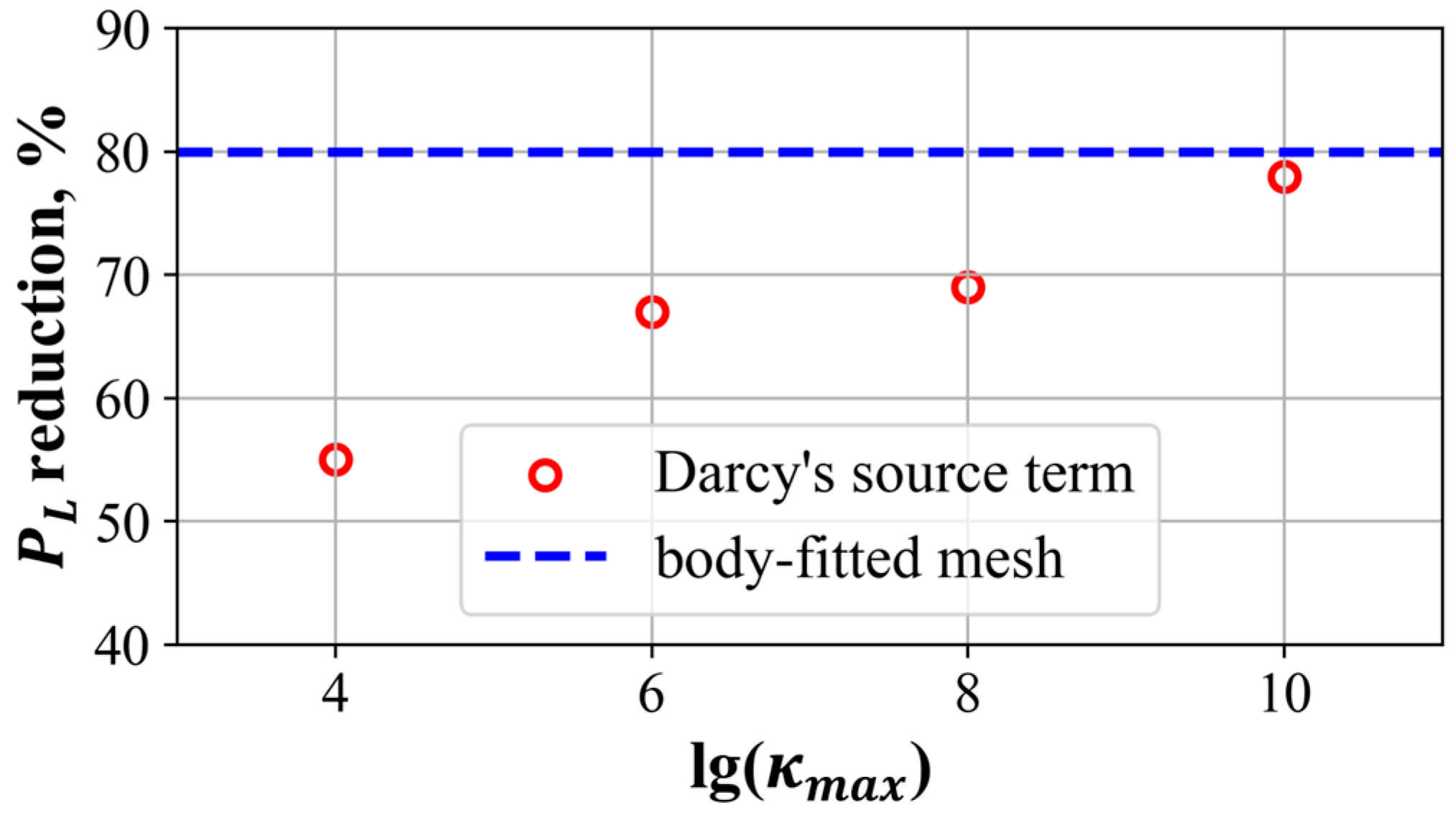
In Figure 28, a body-fitted mesh is generated around the optimized configuration. The of the optimized configuration is computed on this mesh and is compared with the of the original configuration in Table 7. is reduced by 80% in the optimized configuration, showing the effectiveness of TopOpt. Figure 29 shows that as increases, the computed with Darcy’s source term modeling the solid approaches that computed by the body-fitted mesh. This result suggests that the SST model can effectively reflect the influence of solid material represented by Darcy’s source term when is large.
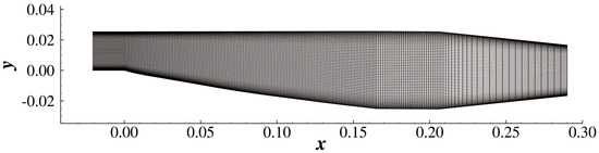
Figure 28.
Body-fitted mesh around the optimized configuration.
Table 7.
comparison.
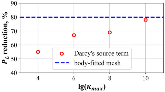
Figure 29.
Variation in , computed in TopOpt with respect to the log of .
Figure 30 shows that the velocity profiles obtained by the optimization mesh + Darcy’s source term and the body-fitted mesh have discrepancies. The cause of the discrepancy is similar to the situation described in Section 5.1.2: the grid resolution around the solid is not enough to resolve wall turbulence during the optimization process.
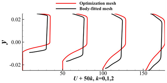
Figure 30.
Velocity profiles obtained by the optimization mesh + Darcy’s source term and the body-fitted mesh + solid-wall boundary.
5.3. Rotor-like Case
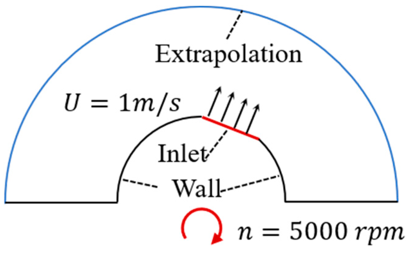
Turbomachinery design is of great importance in the application of aerodynamic optimization. To show the modified SST model’s ability to handle the TopOpt of turbomachinery, a geometry (Figure 31) [10] generalized from a centrifugal compressor (Figure 32) was optimized with the modified SST model. Only one inlet is included in Figure 31, considering the rotational symmetry of the centrifugal compressor. As shown in Figure 31, the whole geometry is in a noninertial frame whose rotation speed is . The rotation effect is considered by adding inertial forces into the momentum equation ():
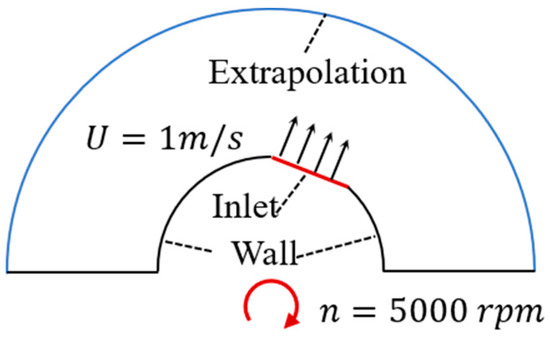
Figure 31.
Computational domain and the boundary conditions.
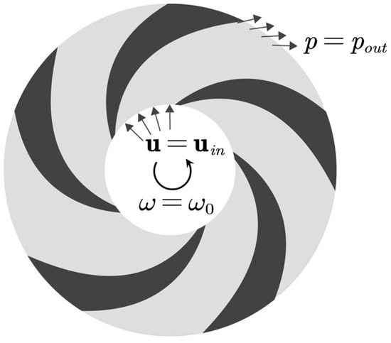
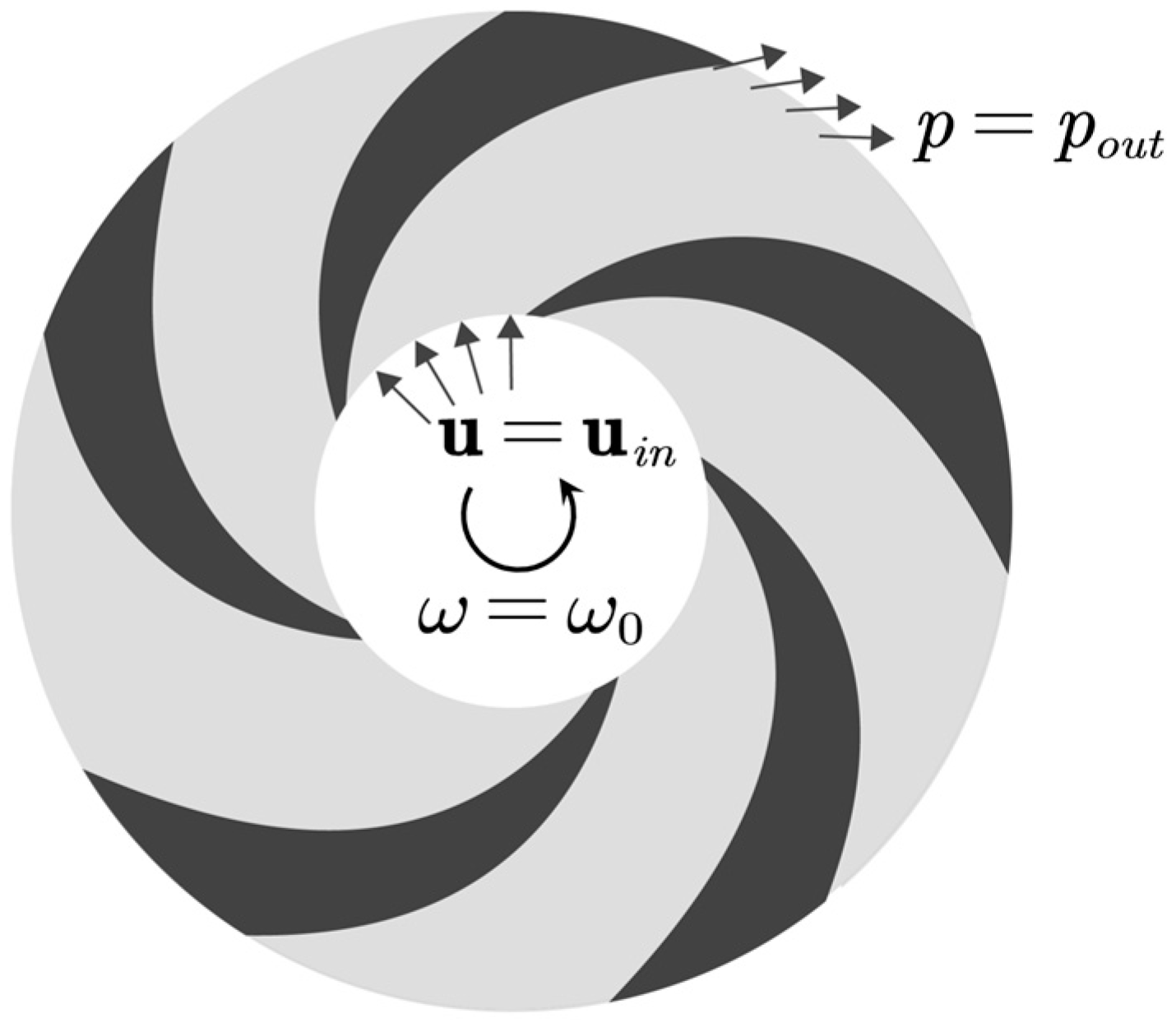
Figure 32.
Illustrative diagram of a centrifugal compressor.
The integral of the dissipation rate over the whole computational domain (see Equation (21)) is chosen as the objective function:
The volume constraint of the solid in Equation (26) is activated with a lower bound of the volume fraction of 0.8:
In the initial condition, is set to 0.8 everywhere to fulfill the constraint. is set to , according to Strategy 1 in Section 2.2.
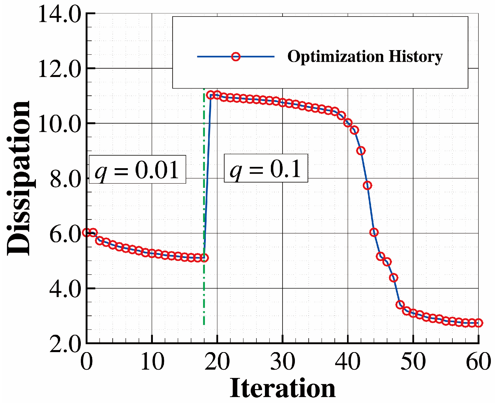
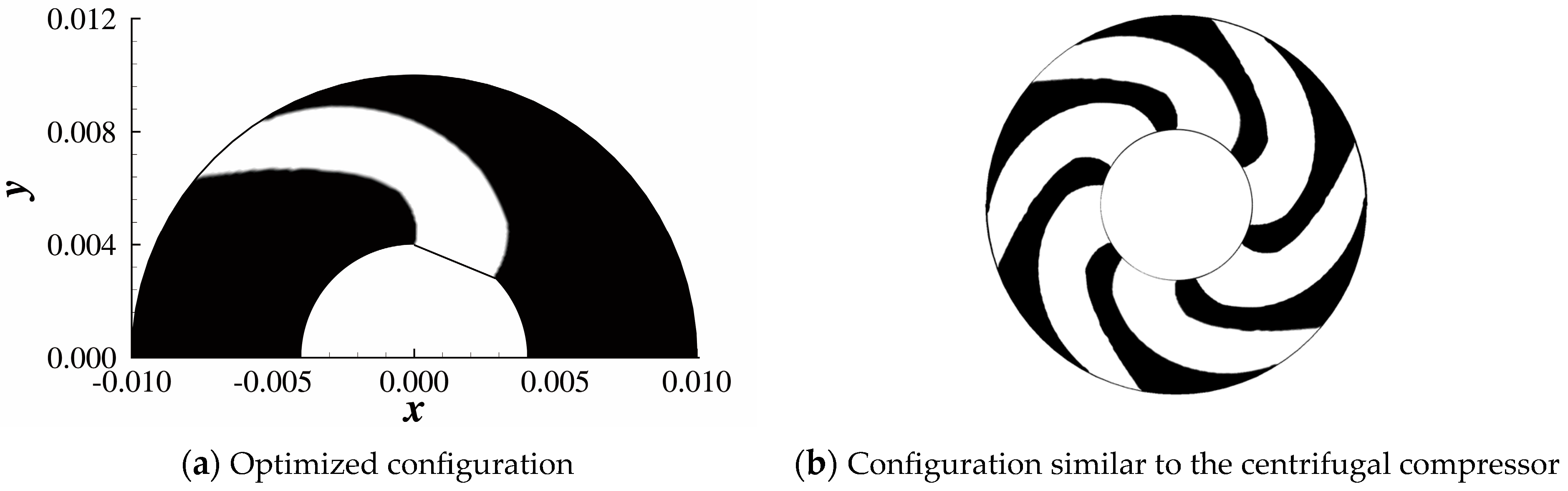
As shown in Figure 33, in Equation (8) is set to 0.01 in the first several iterations. After the optimization converges to a solution where many cells have intermediate values, is increased to 0.1 to make the solid–fluid boundary sharp. This trick was proposed by Borrvall et al. [2]. The optimized configuration, shown in Figure 34a, is a pipe deflected toward the Coriolis force felt by the fluid particles. The pipe is copied and uniformly distributed around the inner circle to obtain a configuration resembling a centrifugal compressor, as shown in Figure 34b. Figure 35 compares the optimized pipe and the velocity field obtained in laminar flow () and the current result. The difference is fairly clear. In the laminar solution, the two sides of the pipe bend in different directions, while in the turbulent solution, both sides bend in the direction of the Coriolis force felt by the fluid particles. The velocity distribution shows that the boundary layer is much thicker in the laminar flow case than in the turbulent flow case. Similar optimization of the rotor in turbulent conditions using the Spalart–Allmaras turbulence model can be found in [17]. In [17], the optimized pipe has two branches, both rooting from the inlet, while in this paper the optimized configuration has one branch only. This is very different from the result of the current case. Many factors can contribute to this difference, including the penalty setting ( and at different stages), the optimizer, the turbulence model, the objective function, and the volume constraint.
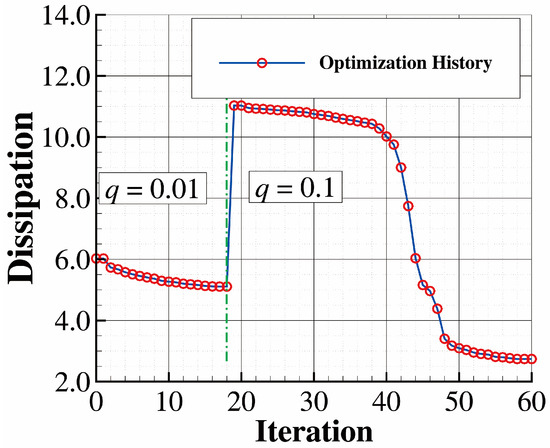
Figure 33.
Convergence history of the energy dissipation.
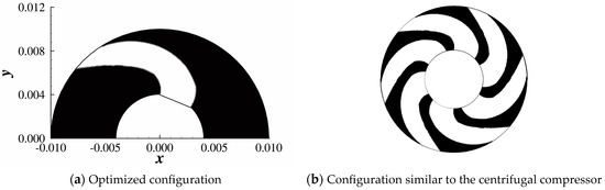
Figure 34.
Result of TopOpt. A curved pipe (the white area) formed after TopOpt.

Figure 35.
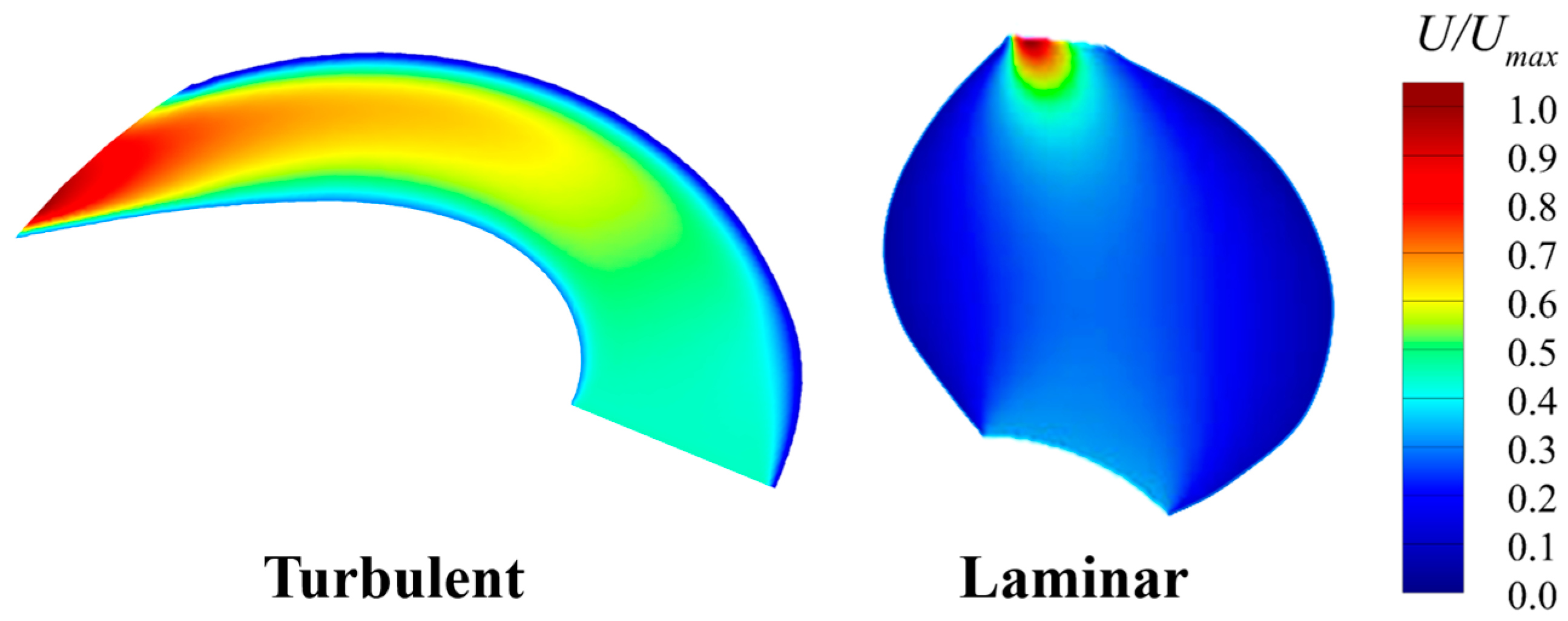
Comparison of the optimized configuration and the velocity distribution in laminar and turbulent flows. The laminar velocity distribution was extracted from [10].
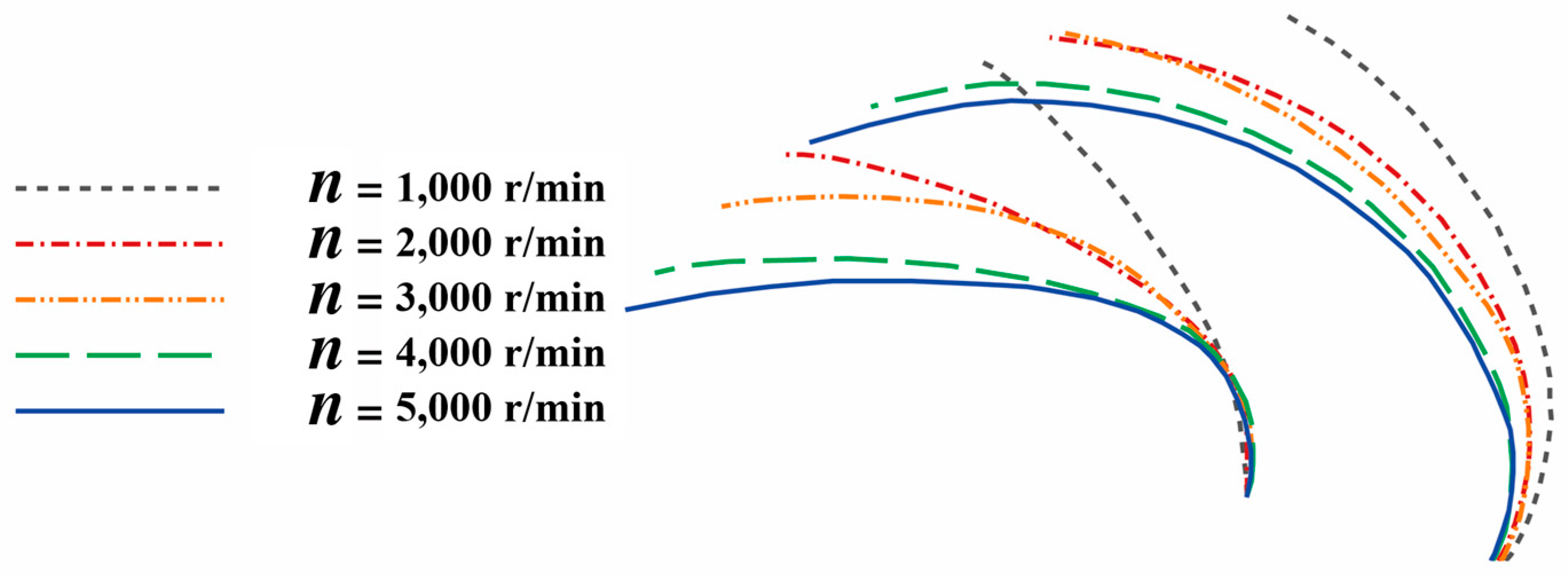
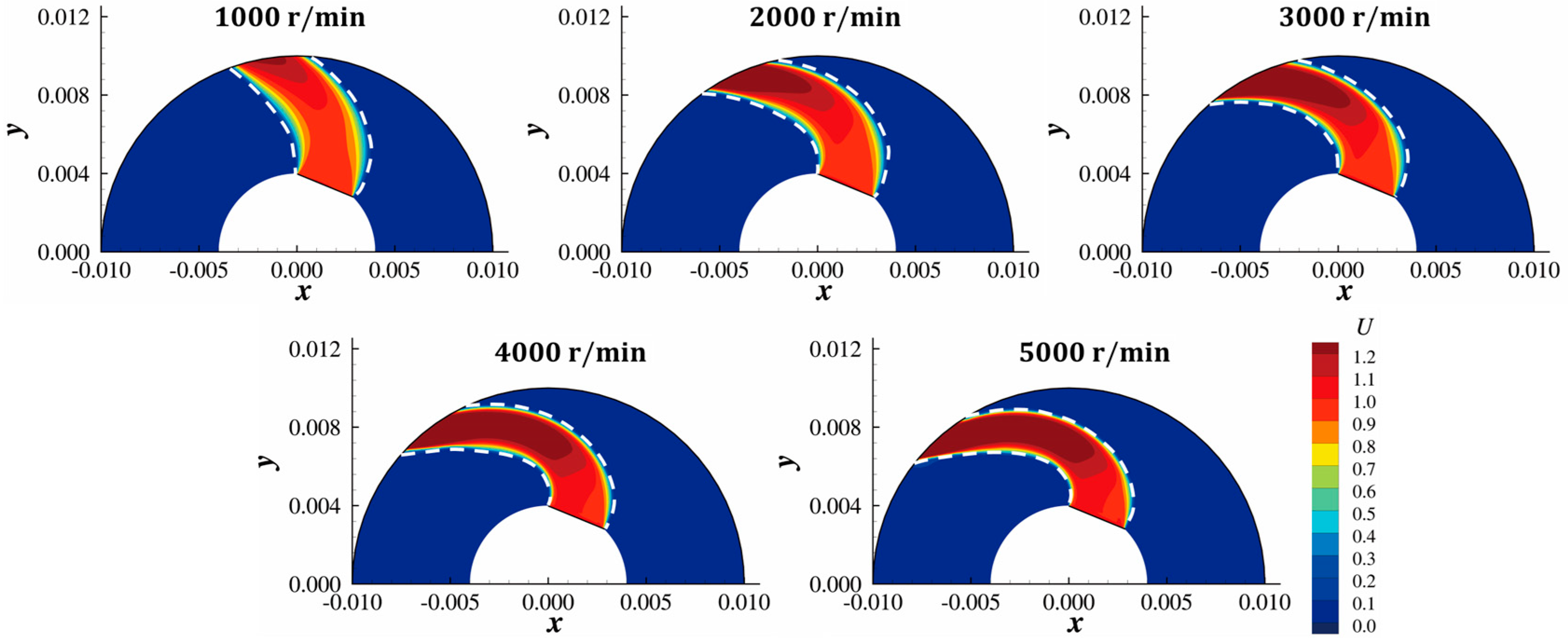
The optimized configurations at other rotating speeds were also computed using TopOpt and are shown in Figure 36. The velocity distribution of the optimized configuration at each rotating speed is shown in Figure 37. All the optimized configurations are pipes deflected in the direction of the Coriolis force, and the larger the rotating speed, the more deflected the pipe. Additionally, the maximum curvature of the pipe is shown to always occur near the inlet.
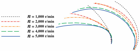
Figure 36.
The optimized configurations are all deflected pipes.

Figure 37.
Velocity magnitude distribution of the optimized configuration at and .
6. Conclusions
The work in this paper focuses on applying TopOpt based on Darcy’s source term to aerodynamic design under turbulent flow. The results and the problems solved can be summarized as follows:
- The minimum needed to impede the fluid flow in a solid (to make in the solid) is proportional to the freestream velocity, , and is unrelated to fluid viscosity when the Reynolds number is large. Based on this relationship and previous experience [18], a strategy for setting is proposed: keep the nondimensional number unchanged when the Reynolds number varies. The strategy is used in the examples of TopOpt and is shown to be effective.
- The flows encountered in aerodynamic design are generally turbulent. Therefore, for TopOpt, considering the impact of Darcy’s source term on turbulence is important. In this paper, a modified LSKE turbulence model is developed. The test case in Section 5.1.2 shows that the proposed model has a satisfactory ability to depict the influence of Darcy’s source term on turbulence, even when the Reynolds number is as high as . A concise, approximate wall-distance computation method that recognizes the solid modeled by Darcy’s source term is developed. This method is integrated into the modified SST model. The modified SST model can also reflect the influence of Darcy’s source term on turbulence when is large.
- Many aerodynamic optimization problems are related to acquiring a configuration with the lowest drag in an external flow. TopOpt was previously mostly used to obtain low-drag profiles in laminar flow. In this study, the TopOpt of a low-drag profile is extended to turbulent flows whose Reynolds numbers are as high as , which has some significance for the application of TopOpt to aerodynamic design.
- Optimizing turbomachinery is another important topic in aerodynamic design. In this paper, the TopOpt of a rotor-like geometry is studied using the modified SST model. The model’s potential for performing the TopOpt of turbomachinery is tested. This test case shows that the larger the rotating speed, the more deflected the optimized configuration.
The authors believe that the problems solved in this work can promote the practical application of TopOpt in the aerodynamic design process, in which high-Reynolds-number turbulent flow is often encountered.
Author Contributions
Conceptualization, C.W. and Y.Z.; methodology, C.W.; software, C.W.; validation, C.W. and Y.Z.; formal analysis, C.W.; investigation, C.W.; resources, Y.Z.; data curation, C.W; writing—original draft preparation, C.W.; writing—review and editing, C.W. and Y.Z.; visualization, C.W.; supervision, Y.Z.; project administration, Y.Z.; funding acquisition, Y.Z. All authors have read and agreed to the published version of the manuscript.
Funding
This work was supported by the National Natural Science Foundation of China (grant nos. 11872230, 92052203, and 91952302) and the Aeronautical Science Foundation of China (grant no. 2020Z006058002).
Data Availability Statement
Dataset available on request from the authors.
Conflicts of Interest
The authors declare no conflict of interest.
References
- Zhang, M.; Liu, J.; Liu, Y. Fluid Topology Optimization Method and Its Application in Turbomachinery. J. Propuls. Technol. 2021, 42, 2401–2416. (In Chinese) [Google Scholar]
- Borrvall, T.; Petersson, J. Topology optimization of fluids in Stokes flow. Int. J. Numer. Methods Fluids 2003, 41, 77–107. [Google Scholar] [CrossRef]
- Gersborg-Hansen, A.; Sigmund, O.; Haber, R.B. Topology optimization of channel flow problems. Struct. Multidiscip. Optim. 2005, 30, 181–192. [Google Scholar] [CrossRef]
- Olesen, L.H.; Okkels, F.; Bruus, H. A high-level programming-language implementation of topology optimization applied to steady-state Navier–Stokes flow. Int. J. Numer. Methods Eng. 2006, 65, 975–1001. [Google Scholar] [CrossRef]
- Each Othmer, C.; De Villiers, E.; Weller, H. Implementation of a continuous adjoint for topology optimization of ducted flows. In Proceedings of the 18th AIAA Computational Fluid Dynamics Conference, Miami, FL, USA, 25–28 June 2007. [Google Scholar]
- Pietropaoli, M.; Montomoli, F.; Gaymann, A. Three-dimensional fluid topology optimization for heat transfer. Struct. Multidiscip. Optim. 2019, 59, 801–812. [Google Scholar] [CrossRef]
- Gaymann, A.; Montomoli, F.; Pietropaoli, M. Fluid topology optimization: Bio-inspired valves for aircraft engines. Int. J. Heat Fluid Flow 2019, 79, 108455. [Google Scholar] [CrossRef]
- Othmer, C. A continuous adjoint formulation for the computation of topological and surface sensitivities of ducted flows. Int. J. Numer. Methods Fluids 2008, 58, 861–877. [Google Scholar] [CrossRef]
- Kondoh, T.; Matsumori, T.; Kawamoto, A. Drag minimization and lift maximization in laminar flows via topology optimization employing simple objective function expressions based on body force integration. Struct. Multidiscip. Optim. 2011, 45, 693–701. [Google Scholar] [CrossRef]
- N. Sá, L.F.; Novotny, A.A.; Romero, J.S.; N. Silva, E.C. Design optimization of laminar flow machine rotors based on the topological derivative concept. Struct. Multidiscip. Optim. 2017, 56, 1013–1026. [Google Scholar] [CrossRef]
- Alexandersen, J.; Andreasen, C.S. A review of topology optimisation for fluid-based problems. Fluids 2020, 5, 29. [Google Scholar] [CrossRef]
- Papoutsis-Kiachagias, E.M.; Kontoleontos, E.A.; Zymaris, A.S.; Papadimitriou, D.I.; Giannakoglou, K.C. Constrained topology optimization for laminar and turbulent flows, including heat transfer. In Proceedings of the EUROGEN, Evolutionary and Deterministic Methods for Design, Optimization and Control, Capua, Italy, 14–16 September 2011; CIRA, Ed.; [Google Scholar]
- Yoon, G.H. Topology optimization for turbulent flow with Spalart–Allmaras model. Comput. Methods Appl. Mech. Eng. 2016, 303, 288–311. [Google Scholar] [CrossRef]
- Dilgen, C.B.; Dilgen, S.B.; Fuhrman, D.R.; Sigmund, O.; Lazarov, B.S. Topology optimization of turbulent flows. Comput. Methods Appl. Mech. Eng. 2018, 331, 363–393. [Google Scholar] [CrossRef]
- Yoon, G.H. Topology optimization method with finite elements based on the k-ε turbulence model. Comput. Methods Appl. Mech. Eng. 2020, 361, 112784. [Google Scholar] [CrossRef]
- Alonso, D.H.; Saenz, J.S.R.; Picelli, R.; Silva, E.C.N. Topology optimization method based on the Wray–Agarwal turbulence model. Struct. Multidiscip. Optim. 2022, 65, 82. [Google Scholar] [CrossRef]
- Sá, L.F.; Yamabe, P.V.; Souza, B.C.; Silva, E.C. Topology optimization of turbulent rotating flows using Spalart–Allmaras model. Comput. Methods Appl. Mech. Eng. 2021, 373, 113551. [Google Scholar] [CrossRef]
- Philippi, B.; Jin, Y. Topology optimization of turbulent fluid flow with a sensitive porosity adjoint method (spam). arXiv 2015, arXiv:1512.08445. [Google Scholar]
- Theulings, M.J.B.; Langelaar, M.; van Keulen, F.; Maas, R. Towards improved porous models for solid/fluid topology optimization. Struct. Multidiscip. Optim. 2023, 66, 133. [Google Scholar] [CrossRef]
- Zhang, M.; Liu, Y.; Yang, J.; Wang, Y. Aerodynamic topology optimization on tip configurations of turbine blades. J. Mech. Sci. Technol. 2021, 35, 2861–2870. [Google Scholar] [CrossRef]
- Launder, B.; Sharma, B. Application of the energy-dissipation model of turbulence to the calculation of flow near a spinning disc. Lett. Heat Mass Transf. 1974, 1, 131–137. [Google Scholar] [CrossRef]
- Wilcox, D.C. Turbulence Modeling for CFD; DCW Industries: La Canada, CA, USA, 1998; Volume 2. [Google Scholar]
- Menter, F.R.; Kuntz, M.; Langtry, R. Ten years of industrial experience with the SST turbulence model. Turbul. Heat Mass Transf. 2003, 4, 625–632. [Google Scholar]
- Menter, F.R. Two-equation eddy-viscosity turbulence models for engineering applications. AIAA J. 1994, 32, 1598–1605. [Google Scholar] [CrossRef]
- OpenFOAM: User Guide: Wall Distance Calculation Methods. (n.d.). Available online: https://www.openfoam.com/documentation/guides/latest/doc/guide-schemes-wall-distance.html (accessed on 16 July 2022).
- Belyaev, A.G.; Fayolle, P. On variational and PDE-based distance function approximations. Comput. Graph. Forum 2015, 34, 104–118. [Google Scholar] [CrossRef]
- He, P.; Mader, C.A.; Martins, J.R.; Maki, K.J. An aerodynamic design optimization framework using a discrete adjoint approach with OpenFOAM. Comput. Fluids 2018, 168, 285–303. [Google Scholar] [CrossRef]
- He, P.; Mader, C.A.; Martins, J.R.R.A.; Maki, K.J. DAFoam: An open-source adjoint framework for multidisciplinary design optimization with OpenFOAM. AIAA J. 2020, 58, 1304–1319. [Google Scholar] [CrossRef]
- He, P.; Mader, C.A.; Martins, J.R.R.A.; Maki, K. An object-oriented framework for rapid discrete adjoint development using OpenFOAM. In Proceedings of the AIAA Scitech 2019 Forum, San Diego, CA, USA, 7–11 January 2019. [Google Scholar]
- Wu, N.; Kenway, G.; Mader, C.A.; Jasa, J.; Martins, J.R.R.A. pyOptSparse: A Python framework for large-scale constrained nonlinear optimization of sparse systems. J. Open Source Softw. 2020, 5, 2564. [Google Scholar] [CrossRef]
- Gill, P.E.; Murray, W.; Saunders, M.A. SNOPT: An SQP algorithm for large-scale constrained optimization. Siam Rev. 2005, 47, 99–131. [Google Scholar] [CrossRef]
- Bradley, A.M. PDE-Constrained Optimization and the Adjoint Method. Technical Report. Stanford University. 2013. Available online: https://cs.stanford.edu/~ambrad/adjoint_tutorial.pdf (accessed on 24 June 2024).
- Duffy, A.C. An Introduction to Gradient Computation by the Discrete Adjoint Method; Technical Report; Florida State University: Tallahassee, FL, USA, 2009. [Google Scholar]
- Li, X.-S.; Gu, C.-W. The momentum interpolation method based on the time-marching algorithm for All-Speed flows. J. Comput. Phys. 2010, 229, 7806–7818. [Google Scholar] [CrossRef]
- Griewank, A.; Walther, A. Evaluating Derivatives: Principles and Techniques of Algorithmic Differentiation; Society for Industrial and Applied Mathematics: Philadelphia, PA, USA, 2008. [Google Scholar]
- Sagebaum, M.; Albring, T.; Gauger, N.R. High-performance derivative computations using codipack. ACM Trans. Math. Softw. 2019, 45, 1–26. [Google Scholar] [CrossRef]
- Philip, E.; Murray, W.; Saunders, M.A. User’s Guide for SNOPT Version 7, a Fortran Package for Large-Scale Nonlinear Programming. 2005. Available online: https://web.stanford.edu/group/SOL/guides/sndoc7.pdf (accessed on 24 June 2024).
- 2D NACA 0012 Airfoil Validation. NASA. Available online: https://turbmodels.larc.nasa.gov/naca0012_val.html (accessed on 24 June 2024).
- Grids-NACA 0012 Airfoil for Turbulence Model Numerical Analysis. Available online: https://turbmodels.larc.nasa.gov/naca0012numerics_grids.html (accessed on 15 January 2023).
- Gregory, N.; O’Reilly, C.L. Low-Speed Aerodynamic Characteristics of NACA 0012 Aerofoil Sections, Including the Effects of Upper-Surface Roughness Simulation Hoar Frost; Reports and Memoranda No. 3726; National Physics Laboratory: Teddington, UK, 1970. [Google Scholar]
- Ladson, C.L. Effects of Independent Variation of Mach and Reynolds Numbers on the Low-Speed Aerodynamic Characteristics of the NACA 0012 Airfoil Section; NASA Technical Memorandum NASA-TM-4074; NASA Langley Research Center: Hampton, VA, USA, 1988.
- 2D Backward Facing Step. Available online: https://turbmodels.larc.nasa.gov/backstep_val.html (accessed on 24 June 2024).
- OpenFOAM: User Guide: Backward Facing Step. Available online: www.openfoam.com/documentation/guides/latest/doc/verification-validation-turbulent-backward-facing-step.html (accessed on 15 January 2023).
- Nasa.gov. 2023. Available online: https://turbmodels.larc.nasa.gov/backstep_validation/profiles.exp.dat (accessed on 15 January 2023).
- OpenFOAM: User Guide: Mesh-Wave Wall Distance. Available online: www.openfoam.com/documentation/guides/latest/doc/guide-schemes-wall-distance-meshwave.html (accessed on 15 January 2023).
- Kulfan, B.M. CST universal parametric geometry representation method with applications to supersonic aircraft. In Proceedings of the Fourth International Conference on Flow Dynamics Sendai International Center Sendai, Sendai, Japan, 26–28 September 2007. [Google Scholar]
- He, P. PitzDaily. DAFoam. 22 February 2022. Available online: https://dafoam.github.io/my_doc_tutorials_topo_pitdaily.html (accessed on 4 April 2022).


Disclaimer/Publisher’s Note: The statements, opinions and data contained in all publications are solely those of the individual author(s) and contributor(s) and not of MDPI and/or the editor(s). MDPI and/or the editor(s) disclaim responsibility for any injury to people or property resulting from any ideas, methods, instructions or products referred to in the content. |
© 2024 by the authors. Licensee MDPI, Basel, Switzerland. This article is an open access article distributed under the terms and conditions of the Creative Commons Attribution (CC BY) license (https://creativecommons.org/licenses/by/4.0/).