Abstract
A novel combination of three control systems is presented in this paper: an adaptive control system, a type-two fuzzy logic system, and a super-twisting sliding mode control (STSMC) system. This combination was developed at the Laboratory of Applied Research in Active Controls, Avionics and AeroServoElasticity (LARCASE). This controller incorporates two methods to calculate the gains of the switching term in the STSMC utilizing the particle swarm optimization algorithm: (1) adaptive gains and (2) optimized gains. This methodology was applied to a nonlinear model of the Cessna Citation X business jet aircraft generated by the simulation platform developed at the LARCASE in Simulink/MATLAB (R2022b) for aircraft lateral motion. The platform was validated with flight data obtained from a Level-D research aircraft flight simulator manufactured by the CAE (Montreal, Canada). Level D denotes the highest qualification that the FAA issues for research flight simulators. The performances of controllers were evaluated using the turbulence generated by the Dryden model. The simulation results show that this controller can address both turbulence and existing uncertainties. Finally, the controller was validated for 925 flight conditions over the whole flight envelope for a single configuration using both adaptive and optimized gains in switching terms of the STSMC.
1. Introduction
Artificial intelligence-based control systems have become the main topic of much research. The recent developments in aircraft systems have increased pilots’ workload; our primary motivation in this paper is to reduce that workload and ease flight procedures for pilots, especially in critical conditions such as atmospheric turbulence. This objective could help to reduce aircraft accidents. As claimed in [1], 80% of aircraft accidents are caused by human errors rather than system failures. The novel methodology proposed here benefits from the advantages of the approximation capability of the Type-Two Fuzzy Logic System (T2FLS) while facing existing uncertainties, the robustness of super-twisting sliding-mode control (STSMC), and the characteristics given by adaptation laws to update approximated functions by a T2FLS during the lateral motion simulation of the Cessna Citation X aircraft in cruise. The gains in the switching control term designed in the STSMC were determined by two different methodologies: one uses adaptation laws, and the other uses the Particle Swarm Optimization method, both of which are discussed in more detail later in this paper.
Concerning the selected methodologies in this article, a brief discussion of the previous studies is presented in this section to provide some essential background. These methodologies have been used for different applications in aerospace and aeronautics.
Satisfying the stability and maneuverability of an aircraft with a control system is essential to guarantee flight safety and passengers’ comfort. These problems have been addressed by a wide range of control techniques and methodologies, as detailed next.
Previously, conventional methodologies showed their compatibility and precision for various types of air vehicles. Idir et al. [2] introduced a novel methodology using a combination of an optimal reduced-order fractional proportional–integral–derivative (PID) controller with the Harris Hawks Optimization Algorithm to control the pitch angle of an aircraft using the Matsuda and the Oustaloup approximation methods. Although these control methodologies have shown superior performance in terms of transient response analysis and the signal characteristics of the pitch angle compared to other controllers, it is necessary to add a robust controller to guarantee the boundedness of the control system, especially in the presence of a load disturbance. To control the pitch of a general aviation aircraft, Deepa and Sudha [3] suggested using tuning methods such as the Zeigler–Nichols, modified Zeigler–Nichols, Tyreus–Luyben, and Astrom–Hagglund methods to find the gains of a PID controller. Based on the presented performance analysis, the Zeigler–Nichols method found more appropriate gain values to remove drastic oscillations, which can be used for both linearized and nonlinear aircraft models. Wilburn et al. [4] developed a new Genetic Algorithm (GA) to optimize the performance of several controllers, including a PID, a Nonlinear Dynamic Inverse (NLDI), and an adaptive PID. The enhanced GA used in this paper benefits from excessive normalization, proposing a mutation operator matrix, varying parameter bounds, and initializing the GA population with predefined values. This study demonstrated that this novel GA algorithm can be used with other controllers, such as artificial immune system-based PID control systems, with the aim of improving the robustness and trajectory tracking performance of an Unmanned Aerial Vehicle (UAV). Moreover, the efficiency of an optimized bio-inspired adaptive control approach with a GA was evaluated in [5] to compensate for aircraft failures. In addition to addressing these failures, that study highlighted the ability of the proposed method to significantly improve aircraft handling qualities. The proposed adaptive immunity-based controllers acted as model-referenced baseline control systems to generate control inputs for the angular rates. This baseline control system and a nonlinear dynamic inversion (NLDI) approach were developed to deal with nonlinearities. Compared with an adaptive neural network system, the combination of the adaptive immunity-based controllers and NLDI provided better results in nominal and abnormal pilot-in-the-loop simulations.
In [6], extensive studies were conducted to evaluate the performance of Linear Quadratic Regulator (LQR), Linear Quadratic Gaussian (LQG), and nonlinear methods for controlling the pitch angle of a UAV. Among these control methods, the LQG successfully attenuated the disturbance, and the LQR performed better under ideal flight conditions. In contrast, the nonlinear control system outperformed both the LQR and LQG methods in terms of smoothness of the response, robustness, and speed of convergence to the reference signal. Further exploration by Vishal and Ohri [7] showed that a Genetic Algorithm (GA) can effectively adjust the parameters of LQR and PID controllers, offering better results in terms of pitch angle control of an aircraft compared to its parameters manual adjustments. Between the GA-based PID controller and the GA-LQR combination, the GA-LQR offered better signal characteristics, such as rise time, settling time, and peak overshoot. In addition, the steady-state error obtained for the GA-LQR was smaller than that of the GA-based PID method. Qi et al. [8] developed a Modified Uncertainty and Disturbance Estimator (MUDE) for achieving accurate attitude-tracking performance in quadcopters using a precise actuation model. This method was compared with cascaded PID and conventional uncertainty and disturbance estimator-based controllers. This comparison revealed that the MUDE-based controller performs better in reducing both tracking and disturbance estimation errors. Furthermore, to solve the path-following problem and attain asymptotic stability for a minimum of three quadrotors, a Robust Load Priority (RLP) control system was proposed in [9]. In this article, a nonlinear control system was developed by leveraging Kane’s method with the direct Lyapunov method to convert the position and attitude errors into a virtual lift control input. This control input helps the quadrotors to rotate and manipulate their loads. On the other hand, a UDE-based robust controller was proposed for a single quadrotor to achieve path-tracking control performance while lifting a suspended payload under disturbances. A two-loop control system was implemented to address external disturbances, such as turbulence, on fixed-wing UAVs flying at low altitudes [10]. It included an LQR and and a Luenberger observer serving as a full-state estimator. In addition to mitigating the effects of disturbances, this control method ensured the safety margin of the UAVs with respect to the ground by tuning the reference altitude. The L1 adaptive control system is another methodology, which was applied in [11] as a fault-tolerant control system to address the challenges caused by actuation failures and turbulence. This control mechanism enhanced the functionalities of a linear controller, and an extended NLDI control system was developed to reduce the distance error with respect to the desired flight path of the West Virginia University Unmanned Aerial Vehicle (UAV). To deal with parameters uncertainties, disturbance, and coupled dynamics in quadrotors, Labbadi et al. [12] have developed super-twisting proportional–integral–derivative sliding-mode control (STPIDSMC) methodologies based on the fractional-order control methodology for each of the position and attitude control systems. This combination offered a highly robust and accurate tracking performance under various scenarios in comparison with fractional-order backstepping sliding-mode control and nonlinear internal control systems by considering their Integral Absolute Error (IAE) values. In addition, to satisfy the 3D trajectory tracking performance of quadcopters, a group of six second-order sliding-mode control (SMC) systems using the super-twisting algorithm within two separate controller mechanisms, one for attitude and altitude of the quadcopters and the other one for the position of the quadcopters, was proposed by Matouk et al. [13]. Compared to a conventional SMC and a fuzzy sliding-mode control system, this control methodology provided improved model robustness to parametric variations, uncertainties, and disturbances and gave more accurate tracking performance without undesired chattering.
In recent years, the evolution of control methodologies has seen a significant shift from conventional approaches to AI-based techniques, demonstrating a broad spectrum of very good adaptability and precision. As an AI-based control system, Deep Recurrent Neural Networks (DRNNs) were used to control highly nonlinear hypersonic vehicles [14], offering very high adaptability to time-varying trajectories and robust performance in the presence of aerodynamic uncertainties. The DRNNs were equipped with gated recurrent units at the hidden neurons to enhance long-term learning and avoid the gradient decay problem. This paper showed that the proposed DRNN-based controller could perform better than the gain-scheduled LQR control approach. This study, among many others, highlights a significant shift from traditional control methods toward exploiting the adaptive capabilities of neural networks. An Aggregated Multiple Reinforcement Learning System (AMRLS) with multiple Reinforcement Learning (RL) algorithms and Cerebellar Model Articulation Controller (CMAC) techniques was proposed in [15] to solve the problem of the exponential increase of dimensionality due to the excessive size of continuous state space equation form used for the pitch control of a B747 aircraft. This control algorithm accelerated the convergence rate and reduced the steady-state pitch error. Furthermore, Andrianantara et al. in [16,17] explored advanced control strategies for the pitch rate control of the Cessna Citation X (CCX) business jet. In [16], a linear PID control system was combined with an adaptive neural network (ANN) and dynamic inversion (DI) methodology to achieve tracking performance and to ensure aircraft stability without prior knowledge of aircraft dynamics. This control methodology gave better results than single PID, PID-DI, and PID-NN control systems. With the same objectives, Andrianantara et al. [17] integrated an adaptive neural network system with an online Recursive Least Square (RLS)-based Model Predictive Controller (MPC) to control the CCX pitch rate under different flight conditions.
According to [18], different controllers, such as PID, fuzzy PID, and sliding-mode control systems, might be chosen for controlling the pitch rate of an aircraft in the presence of unpredicted conditions such as external disturbances. In this article, although the fuzzy PID control system showed the best signal characteristics in terms of tracking performance, besides its ability to update the control parameters during the simulation, the SMC systems worked perfectly in terms of both rise and settling times among all the presented methods. Nair et al. [19] studied the performance of a Linear Quadratic Controller (LQR) system and a Fuzzy Logic Controller (FLC) based on their time response characteristics in controlling the aircraft yaw rate. This study revealed that both methods have specific steady-state errors and overshoots; however, the LQR controller converges to the given desired signals faster than the FLC system. With the aim of achieving a robust automatic landing system in the presence of coupling effects and uncertainties, a proportional–derivative fuzzy logic control system was developed for the nonlinear six-degree-of-freedom models of a medium-sized aircraft. The performance analysis illustrated that this control methodology was appropriate in terms of the stability and steady-state error criteria [20]. Jiao et al. [21] focused on the stability of quadrotor Unmanned Aerial Vehicles (UAVs) equipped with a 2-degree-of-freedom robotic arm and a combination of Sliding-Mode Extended State Observer (SMESO) and a Fuzzy Adaptive Saturation Super-Twisting Extended State Observer (FASTESO) that updated observer gains for the accurate attitude control in the presence of disturbances. In addition, an adaptive super-twisting sliding-mode methodology was developed by Humaidi and Hasan in [22] to control a two-axes helicopter with uncertainties in its model to achieve tracking performance while reducing the chattering on the control input. This control model was equipped with the Particle Swarm Optimization (PSO) algorithm to find the best values for the design parameters.
Dealing with uncertainties is another challenging issue for aircraft control. Hashemi and Botez [23] suggested using a robust adaptive T-S fuzzy logic control system for the Hydra Technologies UAS-S4 Ehécatl to handle various uncertainties, such as unknown parameters in the control system, modelling errors, and disturbances. To minimize energy consumption, improve tracking performance, and maintain stability in a chaotic environment in a Click Mechanism Flapping Wing (CMFW) of an insect-inspired Nano Air Vehicle (NAV), which was defined by T-S fuzzy rules, the authors in [24] proposed using a fuzzy controller integrated with a state feedback control system. In this methodology, the gains of the fuzzy logic-based control system were updated using several adaptive control laws derived from the Lyapunov theorem.
Yu et al. [25] validated the performance of a fault-tolerant control method for UAVs to maintain their attitude with the occurrence of failures in the actuation system while dealing with the existing model uncertainties. This control system employed a fractional-order-based control system based on an adaptive fuzzy neural network system to approximate the uncertainties due to the failures in the follower UAV actuation systems. In addition, distributed sliding-mode systems were designed to estimate the attitudes of the leader UAVs to ensure attitude-tracking performance and to achieve a safe formation. As another fault-tolerant control system for UAVs, a new event-triggered methodology was included using fractional-order calculus and interval type-2 fuzzy neural network systems to satisfy attitude-tracking performance and stability [26]. The stability of the UAVs was demonstrated by analyzing their performance at different attitudes while tracking the issued reference signals. These control systems have reduced the communication load while improving the fault tolerance properties in this application. Moreover, it was suggested in [27] to apply a combination of fixed-time performance functions, fractional calculus, and sliding-mode surfaces, enhanced by recurrent fuzzy neural networks, to keep the tracking errors within certain bounds and improve fault tolerance characteristics of the UAVs in the presence of actuators faults.
Continuing the investigations outlined for the longitudinal motion of a Cessna Citation X using fuzzy logic-based control systems in [28,29] and a model reference adaptive recurrent neural network control system in [30], this study aims to explore their compatibility with the lateral motion of the aircraft, which is more complex than the longitudinal motion due to the coupling between the roll and yaw motions. Therefore, this paper mainly contributes to the application of an artificial intelligence methodology with the Type-Two Adaptive Fuzzy Logic System (T2AFLS) combined with a nonlinear super-twisting sliding-mode control (STSMC) system for the lateral motion of aircraft, as detailed below:
- Previously, most studies were devoted to designing an AI-based controller for the longitudinal motion of aircraft. However, this article presents a new combination of control systems comprising T2AFLS and STSMC methodologies for the lateral motion of the Cessna Citation X aircraft. This methodology addresses two main challenges in the control of an aircraft: (1) the issues that arise with structured uncertainties, such as variations of flight conditions, and unstructured uncertainties, such as unmodeled parameters, and (2) aircraft stabilization in the presence of turbulence. We used the Dryden turbulence model to generate a moderate-intensity turbulence profile, which has not been used before with the considered methodology in the paper. This controller benefits from an improved uncertainty handling offered by the T2FLS, while the adaptation laws determined based on the Lyapunov theorem help to continuously update the approximated function by the fuzzy logic system. Enhanced robustness and stability were achieved using a nonlinear super-twisting sliding-mode control (STSMC). Two methodologies were employed to fine-tune the gains in the STSMC term: (1) adaptive control laws (calculated by the Lyapunov theorem) presented later in this paper [31,32], and (2) the Particle Swarm Optimization (PSO) algorithm. Although the adaptation laws used for the switching control term in this paper were designed based on the methodology proposed in [32], our new method suggests combining the T2AFLS-based approximator with the adaptive super-twisting sliding-mode control, a considerable contribution to the theory. The performances of these approaches are compared to each other to help the reader understand the advantages of each method in this particular application. The validation process was conducted across the entire flight envelope (over 925 flight conditions covering the whole flight envelope) to ensure its reliability and effectiveness with and without turbulence.
- The super-twisting sliding-mode control system (STSMC) has been studied for different aircraft types alone and with other control systems [21,22]. The methodology proposed here is novel according to several features; for example, in [21], the authors combined the Type-One Adaptive Fuzzy Logic System (T1AFLS) with the STSMC, where the T1AFLS was employed to approximate the gain in the switching control term, whereas the proposed Type-Two Adaptive Fuzzy Logic System (T2AFLS) in our paper was used to approximate the unknown dynamics of the aircraft. Furthermore, our controller employs two methodologies to find the gains in the switching control term formulated based on the super-twisting algorithm, the adaptive switching term, and the optimized switching term by using the PSO algorithm. Although the authors in [22] applied the PSO algorithm to optimize those gains, our methodology offers some improvement. Our paper proposes a different cost function to optimize three parameters, which could reduce the computational burden regarding the number of iterations and the swarm population compared with the one used in [22] for optimizing eight parameters.
- We validated our new methodologies using a highly accurate nonlinear simulation platform designed with actual flight data derived from a Level-D Research Aircraft Flight Simulator (RAFS) for Cessna Citation X business aircraft. We believe this simulation platform can precisely represent the dynamics of Cessna Citation X aircraft at each flight phase. This paper is thus among the pioneer articles that applied this methodology to a business aircraft containing much more nonlinearities and complexity than the Unmanned Air Vehicles (UAVs) [21], helicopter models [22], Teledyne Ryan BQM-34 (Firebee) aircraft used in [32], quadrotors [12,13], and hypersonic aircraft [20].
The rest of this article is organized as follows: Section 2 begins with a description of the lateral aircraft model, followed by a detailed explanation of the applied control methodology in Section 2.2. Next, Section 3 discusses the simulation results for each control approach, including a comparison of their performances. This paper will be concluded in Section 4.
2. Methodology
This section explains the methodology for developing a Super-Twisting Adaptive Type-Two Fuzzy Sliding-Mode Control (STAT2FSMC) system. This control system integrates the robustness of a super-twisting control system with the adaptive approximation capability of a Type-Two Adaptive Fuzzy Logic System (T2AFLS). The super-twisting sliding-mode control system (STSMC) is an enhanced type of sliding-mode control system commonly used for mitigating chattering (unwanted oscillations with finite frequency and amplitude) [33].
The nonlinear aircraft model is described in Section 2.1. This model contains unknown dynamics that can be approximated by an Adaptive Type-Two Fuzzy Logic System (AT2FLS). The adaptive characteristic of this approximator is that it fine-tunes the adjustable parameters in real time in order to acquire optimal performance under various flight conditions. A Particle Swarm Optimization (PSO) method was utilized to find the appropriate values for the design parameters of this controller.
2.1. Aircraft Mathematical Model
This article uses a nonlinear model of the Cessna Citation X business jet aircraft. The aircraft is represented by a state-space model to provide adequate understanding and prediction abilities for its response of an aircraft to control inputs and external disturbances. For this purpose, a simulation platform was employed to reproduce the nonlinear lateral dynamics of the Cessna Citation X. This simulation platform was developed at the LARCASE laboratory and validated with flight data obtained from a Level-D Research Aircraft Flight Simulator (RAFS), as shown in Figure 1. Level D is the highest degree of qualification issued by the Federal Aviation Administration (FAA) for research flight simulators [34].
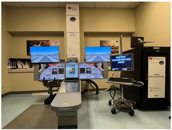
Figure 1.
The Level-D RAFS for the Cessna Citation X business jet aircraft.
The state vector for the aircraft lateral model typically includes variables such as sideslip angle , roll rate , roll angle , and yaw rate . These state variables are the most pertinent for describing the variations of the aircraft dynamics in lateral motion. The main objective of this research is to control the roll rate and to stabilize the yaw rate indirectly by controlling the sideslip angle . Therefore, the state-space representation can be written in a standard form with its order of time derivative, as given in [35]:
where is the state vector, and are the unknown nonlinear functions to be approximated for the purpose of this research, represents the unknown disturbance, and denotes the control inputs, such as the ailerons and rudder command signals.
Practically, represents the control effectiveness. This function exhibits minimal variations in business jets such as the Cessna Citation X during cruise, in which stable and smooth maneuvers are crucial. This aspect was observed during simulation. Thus, to reduce the complexity of the control system design and to focus on the aircraft’s dominant nonlinearities in the presence of uncertainties and turbulence, in this methodology, was approximated to be equal to 1, (), and was approximated by the Type-Two Adaptive Fuzzy Logic System (T2AFLS) using the methodology presented in Section 2.2.1.
2.2. Control System Design
Two control systems are designed here, one for the roll rate and the other one for the yaw rate. The roll rate control system that produced the aileron command signal was designed using a Type-Two Adaptive Fuzzy Super-Twisting Sliding-Mode Control (T2AFSTSMC). In addition, an integral (I) controller was employed to stabilize the yaw rate using the sideslip angle error (the rudder command).
The first step to designing the roll rate control system is to provide the details of the applied Type-Two Fuzzy Logic System, presented next in Section 2.2.1.
2.2.1. Type-Two Fuzzy Logic System as an Approximator
Fuzzy logic systems have emerged as a practical approach to control nonlinear systems in many studies. Unlike conventional control systems, which are designed for crisp input and output values, a fuzzy logic system relies on the linguistic qualification of the input and output values, thus akin to human reasoning, which operates on a spectrum of possibilities.
For the methodology proposed here, the Type-Two Fuzzy Logic system was selected due to its ability to handle uncertainties and variations in aircraft dynamics. The Type-Two Fuzzy Logic System consists of the following 5 components [36]: (1) Fuzzifier, (2) Inference Engine, (3) Fuzzy Rule Base, (4) Type Reducer, and (5) Defuzzifier. A simplified architecture of a Type-Two Fuzzy Logic System is illustrated in Figure 2.
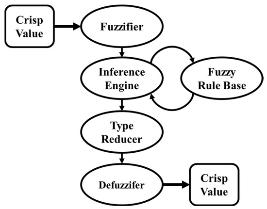
Figure 2.
A simple Type-2 Fuzzy Logic System architecture.
Initially, the inputs must be fuzzified by a membership function showing the membership degree of an input value to a fuzzy set. In this Type-Two Fuzzy Logic System, for each input variable, such as the roll rate and its reference signal , lower and upper membership functions were defined to compose a region called a “Footprint of Uncertainty (FOU)”, as shown in cyan and red colours in Figure 3. The definition of these membership functions improves the handling of uncertainties compared to the single membership function used in Type-One Fuzzy Logic Systems [37].
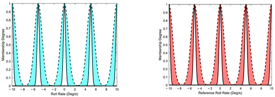
Figure 3.
Upper (dashed line) and lower (solid line) membership functions and the FOU for the roll rate (in cyan) and its reference (in red).
In normal flight conditions, the roll rate varies between −1 and 1 degree per second. However, moderate-intensity turbulence can cause significant fluctuations, resulting in much higher roll rates. To handle this wide range of uncertainties and to ensure smoother maneuvers while maintaining passenger comfort and flight safety, the roll rate linguistic variables were defined between −10 and 10 degrees per second. This range was selected based on standard operational specifications of the CCX aircraft.
The membership functions shown in Figure 3 were selected using five Gaussian membership functions formulated in Equation (2). The parameters of these membership functions are presented in Table 1 with the linguistic terms for each constructed fuzzy set (constructed with upper and lower membership functions). The values of the and given in Table 1 were found on a trial-and-error basis.

Table 1.
Linguistic terms and parameter values of the membership functions.
The relationship between the membership functions can be defined using the IF–THEN rules described in Equation (3):
where are the inputs of the T2FLS, are the membership functions defined for each input, is the output of the T2FLS, and is a singleton fuzzy set for the rule. In this equation, is the number of the inputs, is the number of fuzzy rules, and is the number of membership functions defined for each input variable [38].
To approximate the aircraft dynamics for its lateral motion, two variables were selected as the inputs of the fuzzy logic system: the roll rate and its reference signal . For each value of roll rate signal and its reference signal , five Gaussian membership functions (), calculated with Equation (2), were uniformly distributed between [−10,10] degrees (this range was determined through a process of trial and error based on the obtained results). The fuzzy rules were defined in Table 2 using the linguistic terms explained in Table 1.
Table 2.
Selected fuzzy rules using the linguistic variables of the roll rate and the roll rate reference .
The singleton fuzzy outputs denoted by in Table 2 create the adjustable parameters vectors shown by and in Equation (4). It should be noted that these vectors were initialized with random numbers between [0, 1]. Therefore, the output of the T2FLS can be calculated as follows:
In Equation (4), and contain the singleton fuzzy outputs named as adjustable parameters which are updated during the simulation using the adaptation laws given in Equation (12). In addition, and are the Fuzzy Basis Functions calculated with Equation (5). Having five membership functions for the roll rate and five membership functions for the roll rate reference , and using the product inference engine, there will be 25 fuzzy rules, as ; therefore, .
To obtain the output of the T2FLS, the Nagar–Bardini (NB) algorithm was selected, as it combined the operations of the type reduction with the Defuzzifier components [39,40]. Thus, the output can be calculated as follows Equation (6). In this fuzzy logic system, at each time, there is at least one active fuzzy rule during simulation, as shown above in Equation (4) [38].
The approximated function obtained in Equation (6) will be used in the developed Adaptive Type-Two Fuzzy Super-Twisting Sliding-Mode Control System, which is explained in Section 2.2.2.
2.2.2. Adaptive Type-Two Fuzzy Super-Twisting Sliding Mode Control System
Based on the contributions explained before in Section 1, we selected the sliding-mode control (SMC) system as a nonlinear control methodology to meet the robustness criteria and lead the aircraft dynamics to reach its equilibrium. Super-twisting sliding-mode control is an improved version of the conventional SMC that can compensate for the turbulence and may more effectively improve control system robustness. The sliding surface can be defined as a function of the tracking error, and its first-time derivative is expressed as follows [41]:
where is a design parameter.
Taking the first-time derivative of the sliding surface in Equation (8), and then replacing , written based on Equation (1) with as the selected state variable and as the time-derivative order, yields the following:
By setting in Equation (9), the equivalent control law can be formulated as shown in Equation (10). In this equation, the unknown function was replaced with its approximation calculated by the T2AFLS in Equation (6).
The switching control term in Equation (11a) was selected as proposed in [31], where is an unknown function. Therefore, the aileron control law can be written as given in Equation (11b):
where denotes the saturation function. In contrast with the control input presented in [42] that used , in Equation (11a), we opted to use the saturation function because of its potential to reduce chattering.
In Equation (11a), and are two positive constants whose values were determined using two different approaches. Initially, we employed an adaptive control methodology to continuously adjust its parameters during the simulation. In this approach, the two parameters were increased until the aircraft state variables reached the sliding surface, and then they decreased over time [31]. The second approach is to employ the Particle Swarm Optimization (PSO) algorithm to find optimal values for and , as well as in Equations (10) and (11a).
In the equivalent control law proposed in Equation (10), the term is unknown, while is not measurable in practice. Therefore, the unknown function () can be replaced with the approximated function as in Equation (6) with the expression . As described earlier, can be computed using the adaptation law in Equation (12):
where and .
To ensure the stability and the boundedness of the proposed control law, the Lyapunov theorem was used, as explained below:
Proof of Stability.
As follows, a comprehensive proof of the stability and boundedness of this control system is presented using the well-known Lyapunov theorem. We propose a Lyapunov candidate as a combination of two terms denoted by for the Type-Two Adaptive Fuzzy Sliding-Mode Control [36] and for the super-twisting switching control [31]. Therefore, the Lyapunov candidate can be written as follows:
where
In Equation (14), are two positive constants. Moreover, to prove the stability of the presented supertwisting control law, using the Lyapunov candidate denoted by in Equation (15), it was suggested in [31] to use new state vectors as expressed later in Equation (25).
As demonstrated in [31], if , the matrix will be positive definite. On the other hand, and are also two positive constants. Thus, the Lyapunov candidate for the switching control law will be [31]
where is a real number, and and are two positive constants. In the developed control law given in Equation (10), we know that is unknown, and it was approximated by . For each of the elements in the vector of the adjustable parameter , there is an optimal value, which can be defined as follows:
According to [36,43,44], the unknown functions and are assumed to be bound to positive constants, such as and , respectively, ( and ). As presented in [43], for the adjustable parameter , there will be , which means that is bound to a finite positive constant, such as . In Equation (16), is not a real parameter; it is only used to demonstrate the Lyapunov proof. Using the minimum approximation error given by [45], and the triangular inequality, we obtain [46]
The time derivative of the sliding surface was calculated in Equation (9). Therefore, it can be rewritten such that
Furthermore, it can be assumed that and then , so that from [47]. By substituting and in Equation (18) (in Equation (10) and are unknown, so was then replaced with its approximation denoted by in the expression of the equivalent control law (), the following relationship can be obtained:
Proving the stability and boundedness of the system requires calculation of the time derivative of the Lyapunov candidate denoted by in Equation (14) and in Equation (15). It must be noted that to explain the demonstrations more clearly for , we considered that in Equation (20) and the stability of the will be separately proved by the related Lyapunov candidate later in this section using Equation (15):
Since , we can adopt the adaptation laws designed for and in Equation (12) into the final expression of in Equation (20). Moreover, as indicated in Equation (17), , and the turbulence was assumed to be bound such that . Therefore, Equation (20) can be reformulated as follows:
The expression in Equation (21) was calculated based on the selected Lyapunov candidate for the equivalent control law in the designed Type-Two Adaptive Fuzzy Sliding-Mode System denoted by in Equation (13) (). In addition, to verify the stability of the proposed control methodology, the stability of the switching control term must also be proved by the related Lyapunov candidate introduced by the term in Equation (15) [31,42]. In the super-twisting adaptive sliding-mode control system, it must be considered that in a specific time limit in the presence of bounded perturbation. Within this consideration, The finite-time convergence and stability of the adaptive switching control law u_sw were discussed in detail in [31,32]. According to [31,32], it was explained that with the following expressions for the and :
where
where and are arbitrary positive finite boundaries and is an uncertain function. As proposed in [31,42], it was assumed that using the expression given for in Equation (22b), where is positive function and shows a bounded perturbation with unknown boundaries [31,32]. With these expressions, and considering , becomes [31,32]
Now, it is possible to rearrange in Equation (11a) as follows [42]:
where and are the adaptive gains of switching control law. For the proof of stability, we should define new state vectors, as shown below regarding the methodology presented in [31]:
Calculating the time derivative of Equation (25), we can write the following:
In Equation (22a), we stated that and ; as stated earlier, and are positive finite boundaries. In addition, it was assumed in [31] that . Therefore, , and . Accordingly, Equation (26) can be reformulated as follows [31]:
where are unknown bounds [31,42]. Then, the time derivatives of and given in Equation (15) become [31]
where as , , and . Thus, in [31], it was concluded that becomes
where
where , and . In [31], it was suggested to use the following adaptation laws to update the gains of the switching control law, as shown in Equation (30), as follows:
For the stability proof and to achieve the finite time convergence, it was explained in [31] that for obtaining in Equation (29), . Moreover, in Equation (30), it was shown that ; therefore, by differentiating and choosing , it yields
Having Equation (31) for , and with , then in Equation (29) becomes zero and , proving that the sliding surface and its derivative converge to zero in finite time.
In addition, as shown in the expression of in Equation (30), there is a term that acts as a detector. This term ensures that when exceeds the threshold , the gains and dynamically increase to correct the system trajectory [31]. Conversely, if remains below the threshold , then and start decreasing. This technique also helps reduce the chattering phenomena. In Equation (30), was used to prevent from becoming zero. More details regarding the stability proof and finite time convergence for the adaptation laws introduced in Equation (30) are discussed in [31,32].
Consequently, in [31], it was proven that the following adaptation laws are bound and that the aircraft dynamics are driven to the sliding surface in a finite time . Hence, using the proposed Lyapunov candidate and its expression given in Equations (21) and (29), the following equation can be obtained:
Therefore, it can be concluded that using the final control law shown in Equation (33), approaches zero in finite time, which means that the aircraft is stable, and the error tends to zero while remaining bound within a certain region around the equilibrium. □
With this respect, using the control laws expressed in Equations (10) and (11a) and its adaptive gains and calculated by Equation (30), the final form of the aileron control law becomes
However, as another approach, we also used the PSO algorithm instead of these adaptation laws to find the optimum values of , and in Equation (33), as explained in Section 2.2.3.
2.2.3. A Particle Swarm Optimization (PSO) Algorithm
Here, we explain our application of a PSO optimization algorithm to find the design parameters used in the proposed control system.
Description of the PSO Algorithm
Particle Swarm Optimization (PSO) is a computational method that iteratively finds an optimal solution that minimizes or maximizes a given cost function. The algorithm mimics the behaviour of a set of particles moving in a swarm, each representing a potential solution. In this context, the particles move through a search space to find the optimal solution, using their individual and global experiences. In addition, each particle shares several attributes with the other particles, such as position and velocity, which are updated at each iteration. This strategy enables progressive and efficient convergence toward the optimal solution [48].
The principle of the PSO algorithm can be described with Equation (34); in this algorithm, each particle searches for the best solution using its personal best and the global best [48] solutions:
where is the total number of swarm population; is the undergoing iteration; is the objective or cost function, which must be minimized; and y is a vector of possible solutions (positions).
Based on the definition of the personal best and the global best in Equation (34), the velocity and position of a given particle can be updated by applying the following rules [48,49]:
where are the new velocity and position of the particle, respectively; is the damping inertia; and are learning coefficients (known as acceleration coefficients); and and are random numbers between 0 and 1. The PSO algorithm is presented in Algorithm 1 [48].
| Algorithm 1. General Particle Swarm Optimization (PSO) Algorithm. |
INPUTS:
|
Definition of the Cost Function
In the PSO, the cost function plays an essential role as the objective function that the algorithm tries to optimize. Each PSO particle navigates the search space, recording its personal experience with the aim of minimizing or maximizing the given cost function, depending on the specific problem to be solved. For the PSO algorithm designed in this article, a particular cost function has been selected to find the optimal values of the parameters of the control system ( in Equation (10) and and in Equation (11a)) proposed in Section 2.2.2. This cost function is given in the following equation:
where .
2.2.4. Integral Controller as a Yaw Rate Stabilizer
The interaction between the yaw and roll motions in an aircraft is a crucial aspect that influences the stability and maneuverability of an aircraft. This article highlights the coupling effects between roll and yaw dynamics. The yaw rate variations directly affect the roll rate. Despite the controllers being distinct and decoupled, the aircraft dynamics remain coupled due to aerodynamic interactions between roll and yaw rate dynamics. To minimize the effect of the variations of the yaw rate, we began by using a proportional–integral–derivative (PID) control technique, which has not provided a satisfactory result for the scope of this research. We determined that the integral (I) controller could perform better than the others at this task. Therefore, we focused on using the sideslip angle and its reference signal to indirectly stabilize the yaw rate signal. Specifically, the control input signal given in Equation (38) for the rudder of the Cessna Citation X aircraft (which is controlled with an electrical actuator) was generated based on the error shown in Equation (37) between the actual sideslip angle and a reference value (e.g., equal to zero):
where is a constant gain; this small gain was selected since large gain values led to instability in the aircraft.
This section presented a detailed explanation of the applied methodologies, whose block diagram is shown in Figure 4. The simulation results obtained with this methodology are discussed for the Adaptive Type-Two Fuzzy Super-Twisting Sliding-Mode Control System using both PSO-based and adaptive switching control terms in the next section.
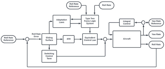
Figure 4.
Simplified scheme of the designed control methodologies.
3. Results
To evaluate the performance of the proposed control system, the nonlinear model of the Cessna Citation X business jet presented in Section 2.1 was used. For this purpose, a total of 925 different flight conditions were selected by varying aircraft weight (lbs), center of gravity position (%) of the chord, altitude (ft), and calibrated airspeed (kts), as shown in Table 3. These 925 flight conditions were selected to cover the entire flight envelope of the Cessna Citation X aircraft.
Table 3.
Parameter values to generate 925 flight conditions.
In the first step, as they are the inputs of the fuzzy system, the roll rate and roll rate reference signals must be fuzzified by the membership function given in Equation (3), whose parameters are defined in Table 3 (these values were found on a trial-and-error basis with respect to the tracking performance of the controller). For each variable, five membership functions were distributed uniformly over the interval of [−10,10] degrees for both upper and lower membership functions for each variable, and , as shown in Table 1.
We decided to follow two different approaches to select the best parameter values used in the sliding-mode switching control term (1) by using the adaptation laws in Equation (30) to find and (the optimal values for the other parameters were chosen by the designer, taking into account the tracking performance) and (2) by using the PSO algorithm described in Section 2.2.3 to find , , and in Equation (33), returning the values presented in Table 4. To find the best values for each of these parameters, we tried different numbers of iterations and population sizes, and it revealed that increasing the number of iterations did not change the results significantly; therefore, the PSO algorithm was designed using the parameters given in Table 4 for both ideal and turbulent flight conditions.
Table 4.
Particle Swarm Optimization configuration.
It should be noted that the bounds and were selected to optimize all three parameters, , , and at the same time. Accordingly, the design parameter values are presented in Table 5 for the T2AFSTSMC with both methodologies, the adaptation laws and the PSO algorithm, as follows. The PSO algorithm was used to determine the values of , and in an offline process, and they remained fixed during the simulation across all flight conditions.
Table 5.
Parameters of the control system design.
The parameter values of the control system design are given in Table 5. Based on the simulation results for 925 flight conditions, the suggested controller could perform adequately in ideal and turbulent conditions. In addition to the signal analysis provided for the obtained results in this section, a more detailed evaluation will be presented next using two tracking error metrics: the Mean Absolute Error (MAE) in Equation (39) and the Max Absolute Error, which is calculated for each flight condition to understand better the performance achieved by each control system. These assessments will be presented later in this section.
As shown in Figure 5, the controller with both types of switching terms could meet the tracking performance, as the roll rate could follow the reference signal. However, the T2AFSTSMC, equipped with an adaptive switching term, could perform slightly better than the PSO-based T2AFSTSMC in tracking the roll rate reference signal. This better performance of the adaptive switching term was achieved because the adaptation laws were able to stabilize the aircraft more effectively by updating the gain values during the simulation rather than by using the fixed parameters found by the PSO.
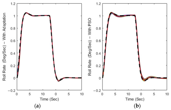
Figure 5.
Roll rate variations for T2AFSTSMC with (a) adaptive switching control term and (b) PSO algorithm (The black dashed line represents the reference signal).
As indicated in Figure 5, the results seem to be similar. Therefore, to determine which method performed better in the control of the roll rate of the Cessna Citation X aircraft, another evaluation is presented in Figure 6, based on the reference signal tracking. This figure shows that the T2AFSTSMC with adaptive switching control can perform better than the PSO-based one in ideal flight conditions, as the Mean Absolute Error (MAE) values (in black) were negligible and consistently smaller than those obtained with the PSO algorithm.
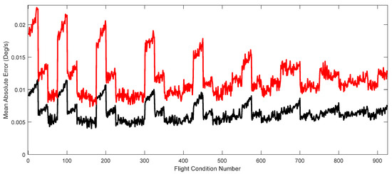
Figure 6.
Mean absolute error for the T2AFSTSMC with adaptive switching control term (black) and the PSO algorithm (red) for each flight condition in ideal condition.
In addition, the performance of the control system was assessed in terms of roll angle variations, as shown in Figure 7. This figure clearly indicates that the aircraft is turning with the roll rate commanded from zero to five degrees. However, there is a discrepancy between the actual roll angle and its reference values after 6 s. Such an issue can be expected since the aircraft was experiencing some residual yaw that was induced by the motion of the aircraft. The difference between the roll angle and its reference signal in the controller with adaptive switching terms was slightly smaller than the PSO-based one. This study required a high level of roll rate tracking performance, which was successfully achieved.
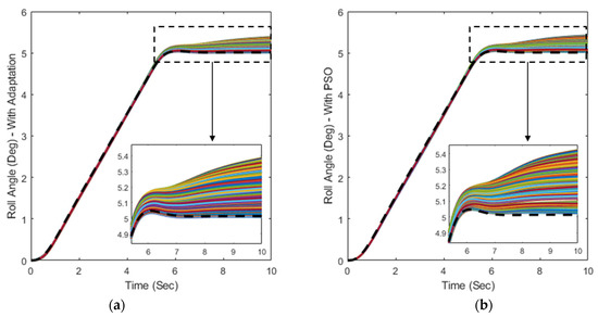
Figure 7.
Roll angle variations for the T2AFSTSMC with (a) adaptive switching control term and (b) PSO algorithm (The black dashed line represents the reference signal).
Designing a control system to generate a smooth control input signal is crucial for several reasons, primarily in terms of passenger safety and comfort and to ensure that commands will not damage the actuation system. Sudden or abrupt maneuvers could lead to structural damage to the airframe and to accelerated wear and tear. In addition, from the flight dynamics approach, smooth commands help to maintain the stability and maneuverability of an aircraft. Our goal was to design a control system that produced a control input signal for ailerons with the most negligible high-frequency oscillations. As shown in Figure 8, both control methodologies could satisfy this criterion. However, the controller with the adaptive switching control term was smoother than the one with PSO, especially during the first seconds of the simulation, as some abrupt changes (in some flight conditions) can be seen between to s.
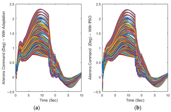
Figure 8.
Time variations of the aileron command for T2AFSTSMC with (a) adaptive switching control term and (b) the PSO-based one.
As shown in Figure 9, to stabilize the yaw rate, we used an integral controller to reduce the steady-state error between the sideslip angle and its trim value (which usually equals zero—black dashed line). By maintaining the sideslip angle close to its trim value, it would be possible to ensure that the yaw rate is stable, as any variations in the sideslip angle can change the yaw rate.
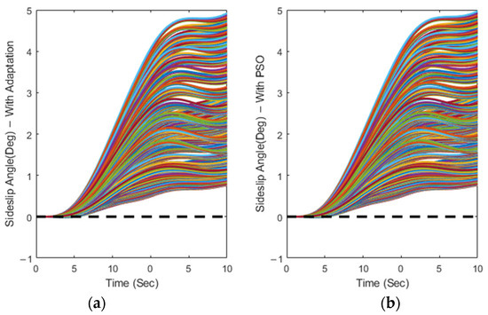
Figure 9.
Time variations of the sideslip angle for T2AFSTSMC with (a) adaptive switching control term and (b) the PSO-based one.
As illustrated in Figure 10, the use of an integral feedback for the sideslip angle allowed the yaw rate variations to be maintained in a reduced range close to zero. These results validate the proposed strategy and demonstrate the effectiveness of the complete control system proposed in this paper.
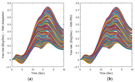
Figure 10.
Time variations of the yaw rate for T2AFSTSMC with (a) adaptive switching control term and (b) the PSO-based one.
One of the main objectives of this research was to design a control system for minimizing the effects of turbulence as a common critical condition during the cruise. To evaluate such systems, we used the Dryden turbulence model available in the Simulink Aerospace Blockset to obtain the effects of turbulence on the performance of Cessna Citation X aircraft equipped with the proposed T2AFSTSMC controllers. To achieve the objectives of this research, we selected the moderate probability for exceedance of high-altitude intensity (equal to ) in accordance with the specifications given in MIL-F-8785C [50].
Earlier in this section, we analyzed the performance of control methodologies under ideal conditions, demonstrating their efficiency and reliability. However, a test of the robustness and adaptability of an aircraft control system lies in its ability to handle real-world phenomena such as turbulence while maintaining the aircraft stability. This analysis highlights the capabilities of the designed control systems and provides precious insights to ensure optimal performance under operational conditions.
As represented in Figure 11, the tracking performance was achieved with both control system methods handling the turbulence effects with a minimum amplitude variation.
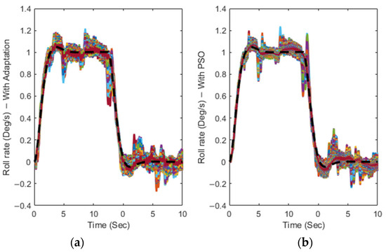
Figure 11.
Time variations of the roll rate for T2AFSTSMC with (a) adaptive switching control term and (b) the PSO-based one (The black dashed line represents the reference signal).
The simulation results in Figure 11 are numerically compared with those shown in Figure 12 at each flight condition, revealing that the MAE values varied in almost the same range using the T2AFSTSMC with an adaptive switching term and with a PSO-based switching term. The trend of these variations shows that as the altitude increased, the MAE values consistently decreased (the first flight condition had the lowest altitude (8000 ft), and the 925th flight condition had the highest altitude (45,000 ft)), indicating that the controller could operate better at higher altitudes than at lower altitudes.
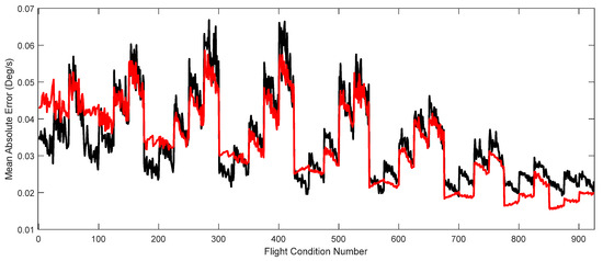
Figure 12.
MAEs for T2AFSTSMC using an adaptive switching term (black) and a PSO-based switching term (red) for each flight condition with turbulence.
While the trends of MAE variations are presented in Figure 12, it was not obvious which method could operate better in the presence of turbulence. To investigate any possible differences, the distribution of the MAEs across all flight conditions was assessed, as shown by the histogram in Figure 13. This evaluation showed that the controller with a PSO-based switching term operated better than the one with an adaptive term, as the MAE values for all flight conditions were less than 0.06 degrees per second. However, the maximum MAE for the controller with an adaptive switching term was very close to this value at less than 0.07 deg/s.
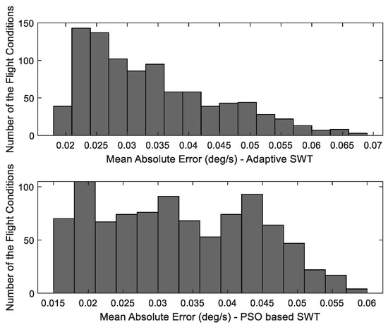
Figure 13.
Distribution of the MAEs for T2AFSTSMC using an adaptive switching term (UP) and a PSO-based switching term (down) under turbulence in 925 flight conditions.
As shown in Figure 14, the aircraft equipped with both switching terms attempted to achieve the commanded roll angle of 5 degrees. However, due to the erratic effects of the turbulence, the roll angle deviated from its reference roll angle, and the aircraft could not remain stable at the targeted 5 degrees. These challenging variations imposed on the maneuverability of the aircraft have occurred in both control methodologies.
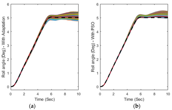
Figure 14.
Roll angle time variations for T2AFSTSMC with turbulence using (a) an adaptive switching term and (b) a PSO-based switching term (The black dashed line represents the reference signal).
As shown in Figure 15, the produced aileron control input signals had minimum abrupt oscillations (without high amplitude) in the presence of turbulence. This characteristic was successfully achieved with both methods since the imposed effects of the turbulence forced the control system to change the position of the ailerons very rapidly within a restricted deviation range.
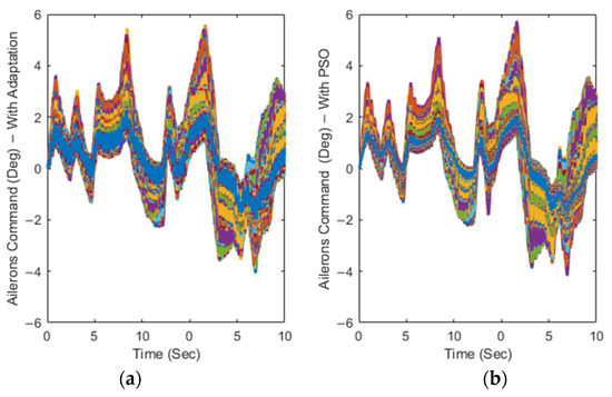
Figure 15.
Time variations of the aileron command for T2AFSTSMC under turbulence with (a) an adaptive switching control term and (b) a PSO-based switching term.
4. Conclusions
In this work, an enhanced Type-Two Adaptive Fuzzy Super-Twisting Sliding-Mode Control system was developed and validated with the nonlinear lateral model of the Cessna Citation X business jet aircraft. In this control system, the Type-Two Fuzzy Logic System approximated the unknown function in the state-space model of the aircraft with no prior knowledge of its parameters. This approximated function could be updated during the simulation using the adaptation laws derived from the Lyapunov theorem. This methodology helped to handle the uncertainties and parameter variations effectively. Both robustness and stability were achieved using the proposed super-twisting sliding-mode control system for the Cessna Citation X aircraft. Principally, in the sliding-mode control, the control law consisted of an equivalent control law based on the concept of the proposed Type-Two Adaptive Fuzzy System and the switching control law. Two methods were employed to choose the best gains values in the switching control law: one with the adaptation laws developed for the gains by the Lyapunov theorem and the other with the gains found by the PSO algorithm. The simulation results revealed that both control approaches were able to guarantee the robustness and stability of the aircraft in the presence of turbulence with a moderate intensity . Furthermore, the tracking performance of the roll rate was excellent while producing the aileron control input with minimum high-frequency oscillations to avoid mechanical damage to the aircraft actuation system. Regarding the tracking performance analyzed for the aircraft roll rate, it was found that the controller equipped with a PSO-based switching control term operated better than the adaptive one, with a maximum Mean Absolute Error (MAE) value equal to 0.06 degrees per second in the presence of turbulence. Finally, this controller could be applied for any aircraft model, as no knowledge regarding the aircraft model or the dynamic parameters is required, and the Adaptive Type-Two Fuzzy Logic System can update the aircraft dynamics in real time with only a measured state variable, such as the roll rate and its reference signal.
Author Contributions
Conceptualization, S.M.H.; Methodology, S.M.H., I.B., G.G. and R.M.B.; Software, S.M.H. and I.B.; Validation, S.M.H. and G.G.; Formal analysis, I.B.; Investigation, S.M.H. and I.B.; Resources, G.G. and R.M.B.; Writing—original draft, S.M.H.; Writing—review & editing, G.G. and R.M.B.; Supervision, G.G. and R.M.B.; Project administration, G.G. and R.M.B.; Funding acquisition, G.G. and R.M.B. All authors have read and agreed to the published version of the manuscript.
Funding
This research was funded by the Canada Research Chair of Aircraft Modelling and New Simulation Technologies, grant number: 231679, which helped in the realization and publication of this article. Ruxandra Botez is the Canada Research Chair Tier 1 Holder in Aircraft Modeling and New Simulation Technologies.
Data Availability Statement
The data presented in this study are available in the article.
Acknowledgments
For more information related to this research, please visit the LARCASE website at https://larcase.etsmtl.ca (accessed on 26 June 2024). This research was performed and realized at the Laboratory of Applied Research in Active Controls, Avionics and AeroServoElasticity (LARCASE). The Research Aircraft Flight Simulator (RAFS) of the Cessna Citation X was obtained by Ruxandra Botez, Full Professor. We give our thanks to research grants from the Canadian Foundation of Innovation (CFI) and the Ministère du Développement Économique, de l’Innovation et de l’Exportation (MDEIE), as well as from the contributions of CAE Inc. The authors would like to thank the CAE Inc. team and Oscar Carranza Moyao for their support in the development of the RAFS at the LARCASE laboratory. Thanks are also due to Odette Lacasse of the ETS for her support.
Conflicts of Interest
The authors declare no conflict of interest.
Nomenclature
| Unknown dynamics function | |
| d(t) | Atmospheric turbulence |
| Aileron command signal (degree) | |
| Rudder command signal (degree) | |
| Aircraft state vector | |
| Sideslip angle (degree) | |
| Roll rate (degree per second) | |
| Roll rate reference (degree per second) | |
| Yaw rate (degree per second) | |
| Fuzzy membership function | |
| Approximated dynamics function | |
| Fuzzy adjustable parameters vector | |
| Fuzzy Basis Functions (FBFs) | |
| Roll rate tracking error | |
| Sliding surface for the lateral motion | |
| , , | Positive design parameters |
| Equivalent control law | |
| Switching control law | |
| , , | Positive gains in the super-twisting switching control law |
| Proposed Lyapunov candidate | |
| Lyapunov term for the Type-Two Adaptive Fuzzy System | |
| Lyapunov term for the adaptive super-twisting switching control law | |
| Minimum approximation error | |
| , , , , | Positive design parameters |
| Personal best in the PSO algorithm | |
| Global best in the PSO algorithm | |
| , , | Uncertain functions |
| , | Arbitrary positive finite boundaries for and |
| Assumed state vector | |
| , | Positive constants |
| s | Iterations in the PSO |
| J | Number of swarm particles |
| , | Lowest and highest bounds of decision variables |
| Damping inertia in the PSO | |
| Personal acceleration in the PSO | |
| Social acceleration in the PSO | |
| Scaling factor for the particle’s velocity in the PSO |
References
- Rankin, W. MEDA Investigation Process. Aeromagazine, ChapterQTR_02, 26. 2007, pp. 15–21. Available online: http://www.lb.boeing.com/commercial/aeromagazine/articles/qtr_2_07/ (accessed on 7 May 2023).
- Idir, A.; Bensafia, Y.; Khettab, K.; Canale, L. Performance Improvement of Aircraft Pitch Angle Control Using a New Reduced Order Fractionalized PID Controller. Asian J. Control 2023, 25, 2588–2603. [Google Scholar] [CrossRef]
- Deepa, S.N.; Sudha, G. Longitudinal Control of Aircraft Dynamics Based on Optimization of PID Parameters. Thermophys. Aeromech. 2016, 23, 185–194. [Google Scholar] [CrossRef]
- Wilburn, B.K.; Perhinschi, M.G.; Wilburn, J.N. A Modified Genetic Algorithm for UAV Trajectory Tracking Control Laws Optimization. Int. J. Intell. Unmanned Syst. 2014, 2, 58–90. [Google Scholar] [CrossRef]
- Perez, A.E.; Moncayo, H.; Perhinschi, M.; Al Azzawi, D.; Togayev, A. A Bio-Inspired Adaptive Control Compensation System for an Aircraft Outside Bounds of Nominal Design. J. Dyn. Syst. Meas. Control. 2015, 137, 091012. [Google Scholar] [CrossRef]
- Ingabire, A.; Sklyarov, A.A. Control of Longitudinal Flight Dynamics of a Fixedwing UAV Using LQR, LQG and Nonlinear Control. E3S Web Conf. 2019, 104, 02001. [Google Scholar] [CrossRef]
- Vishal; Ohri, J. GA Tuned LQR and PID Controller for Aircraft Pitch Control. In Proceedings of the 2014 IEEE 6th India International Conference on Power Electronics (IICPE), Kurukshetra, India, 8–10 December 2014. [Google Scholar] [CrossRef]
- Qi, Y.; Zhu, Y.; Wang, J.; Shan, J.; Liu, H.H.T. MUDE-Based Control of Quadrotor for Accurate Attitude Tracking. Control Eng. Pract. 2021, 108, 104721. [Google Scholar] [CrossRef]
- Qian, L.; Liu, H.H.T. Robust Control Study for Tethered Payload Transportation Using Multiple Quadrotors. J. Guid. Control Dyn. 2022, 45, 434–452. [Google Scholar] [CrossRef]
- Xiong, S.; Liu, H.H.-T. Low-Altitude Fixed-Wing Robust and Optimal Control Using a Barrier Penalty Function Method. J. Guid. Control Dyn. 2023, 46, 11. [Google Scholar] [CrossRef]
- Moncayo, H.; Krishnamoorty, K.; Wilburn, B.; Wilburn, J.; Perhinschi, M.; Lyons, B. Performance Analysis of Fault Tolerant UAV Baseline Control Laws with L1 Adaptive Augmentation. J. Model. Simul. Identif. Control 2013, 1, 137–163. [Google Scholar] [CrossRef]
- Labbadi, M.; Boukal, Y.; Cherkaoui, M. Path following Control of Quadrotor UAV with Continuous Fractional-Order Super Twisting Sliding Mode. J. Intell. Robot. Syst. 2020, 100, 1429–1451. [Google Scholar] [CrossRef]
- Matouk, D.; Abdessemed, F.; Gherouat, O.; Terchi, Y. Second-order sliding mode for position and attitude tracking control of quadcopter UAV: Super-twisting algorithm. Int. J. Innov. Comput. Inf. Control IJICIC 2020, 16, 29–43. [Google Scholar] [CrossRef]
- Nivison, S.A.; Khargonekar, P.P. Development of a Robust Deep Recurrent Neural Network Controller for Flight Applications. In Proceedings of the 2017 American Control Conference (ACC), Seattle, WA, USA, 24–26 May 2017. [Google Scholar] [CrossRef]
- Jiang, J.; Kamel, M.S. Pitch Control of an Aircraft with Aggregated Reinforcement Learning Algorithms. In Proceedings of the 2007 International Joint Conference on Neural Networks, Orlando, FL, USA, 12–17 August 2007. [Google Scholar] [CrossRef]
- Andrianantara, R.P.; Ghazi, G.; Botez, R.M. Neural Network Adaptive Controller with Approximate Dynamic Inversion for Pitch Control of the Cessna Citation X. In Proceedings of the AIAA AVIATION 2023 Forum, San Diego, CA, USA and Online, 12–16 June 2023. [Google Scholar] [CrossRef]
- Andrianantara, R.P.; Ghazi, G.; Botez, R.M. Model Predictive Controller with Adaptive Neural Networks and Online State Estimation for Pitch Rate Control of the Cessna Citation X. In Proceedings of the AIAA SCITECH 2024 Forum, Orlando, FL, USA, 8–12 January 2024. [Google Scholar] [CrossRef]
- Khalid, A.; Zeb, K.; Haider, A. Conventional PID, Adaptive PID, and Sliding Mode Controllers Design for Aircraft Pitch Control. In Proceedings of the 2019 International Conference on Engineering and Emerging Technologies (ICEET), Lahore, Pakistan, 21–22 February 2019. [Google Scholar] [CrossRef]
- Nair, V.G.; George, V.I. Aircraft Yaw Control System Using LQR and Fuzzy Logic Controller. Int. J. Comput. Appl. 2012, 45, 9. [Google Scholar]
- Nho, K.; Agarwal, R.K. Automatic Landing System Design Using Fuzzy Logic. J. Guid. Control Dyn. 2000, 23, 298–304. [Google Scholar] [CrossRef]
- Jiao, R.; Chou, W.; Rong, Y.; Dong, M. Anti-Disturbance Control for Quadrotor UAV Manipulator Attitude System Based on Fuzzy Adaptive Saturation Super-Twisting Sliding Mode Observer. Appl. Sci. 2020, 10, 3719. [Google Scholar] [CrossRef]
- Humaidi, A.J.; Hasan, A.F. Particle Swarm Optimization–Based Adaptive Super-Twisting Sliding Mode Control Design for 2-Degree-of-Freedom Helicopter. Meas. Control 2019, 52, 1403–1419. [Google Scholar] [CrossRef]
- Hashemi, S.M.; Botez, R.M. Lyapunov-Based Robust Adaptive Configuration of the UAS-S4 Flight Dynamics Fuzzy Controller. Aeronaut. J. 2022, 126, 1187–1209. [Google Scholar] [CrossRef]
- Hashemi, S.M.; Botez, R.M.; Grigorie, L.T. Adaptive Fuzzy Control of Chaotic Flapping Relied upon Lyapunov-Based Tuning Laws. In Proceedings of the AIAA AVIATION 2020 FORUM, Virtual Event, 15–19 June 2020. [Google Scholar] [CrossRef]
- Yu, Z.; Zhang, Y.; Liu, Z.; Qu, Y.; Su, C.-Y. Distributed Adaptive Fractional-Order Fault-Tolerant Cooperative Control of Networked Unmanned Aerial Vehicles via Fuzzy Neural Networks. IET Control Theory Appl. 2019, 13, 2917–2929. [Google Scholar] [CrossRef]
- Yu, Z.; Yang, Z.; Sun, P.; Zhang, Y.; Jiang, B.; Su, C.-Y. Refined Fault Tolerant Tracking Control of Fixed-Wing UAVs via Fractional Calculus and Interval Type-2 Fuzzy Neural Network under Event-Triggered Communication. Inf. Sci. 2023, 644, 119276. [Google Scholar] [CrossRef]
- Yu, Z.; Zhang, Y.; Jiang, B.; Su, C.-Y.; Fu, J.; Jin, Y.; Chai, T. Enhanced Recurrent Fuzzy Neural Fault-Tolerant Synchronization Tracking Control of Multiple Unmanned Airships via Fractional Calculus and Fixed-Time Prescribed Performance Function. IEEE Trans. Fuzzy Syst. 2022, 30, 4515–4529. [Google Scholar] [CrossRef]
- Hosseini, S.; Ghazi, G.; Botez, R.M. Design of a Type Two Fuzzy-Based System to Control the Pitch Rate of the Cessna Citation X. In Proceedings of the AIAA AVIATION 2023 Forum, San Diego, CA, USA and Online, 12–16 June 2023. [Google Scholar] [CrossRef]
- Hosseini, S.; Ghazi, G.; Botez, R.M. Application of Type One Adaptive Fuzzy Sliding Mode Control System for the Longitudinal Motion of the Cessna Citation X. In Proceedings of the AIAA AVIATION 2023 Forum, San Diego, CA, USA and Online, 12–16 June 2023. [Google Scholar] [CrossRef]
- Hosseini, S.; Inga, C.; Ghazi, G.; Botez, R.M. Model-Referenced Adaptive Flight Controller Based on Recurrent Neural Network for the Longitudinal Motion of Cessna Citation X. In Proceedings of the AIAA AVIATION 2023 Forum, San Diego, CA, USA and Online, 12–16 June 2023. [Google Scholar] [CrossRef]
- Shtessel, Y.; Taleb, M.; Plestan, F. A Novel Adaptive-Gain Supertwisting Sliding Mode Controller: Methodology and Application. Automatica 2012, 48, 759–769. [Google Scholar] [CrossRef]
- Yan, B.; Dai, P.; Liu, R.; Xing, M.; Liu, S. Adaptive Super-Twisting Sliding Mode Control of Variable Sweep Morphing Aircraft. Aerosp. Sci. Technol. 2019, 92, 198–210. [Google Scholar] [CrossRef]
- Utkin, V.; Lee, H. Chattering problem in sliding mode control systems. IFAC Proc. Vol. 2006, 39, 1. [Google Scholar] [CrossRef]
- Ghazi, G.; Botez, R.; Messi Achigui, J. Cessna Citation X Engine Model Identification from Flight Tests. SAE Int. J. Aerosp. 2015, 8, 203–213. [Google Scholar] [CrossRef]
- Yedavalli, R.K. Flight Dynamics and Control of Aero and Space Vehicles; John Wiley & Sons: Hoboken, NJ, USA, 2020. [Google Scholar]
- Wang, L.-X. A Course in Fuzzy Systems and Control; Prentice Hall PTR: Upper Saddle River, NJ, USA, 1997. [Google Scholar]
- Hagras, H.; Wagner, C. Towards the Wide Spread Use of Type-2 Fuzzy Logic Systems in Real World Applications. IEEE Comput. Intell. Mag. 2012, 7, 14–24. [Google Scholar] [CrossRef]
- Wang, L.-X. Adaptive Fuzzy Systems and Control: Design and Stability Analysis; PTR Prentice Hall: Upper Saddle River, NJ, USA, 1994. [Google Scholar]
- Chen, Y. Study on Centroid Type-Reduction of Interval Type-2 Fuzzy Logic Systems Based on Noniterative Algorithms. Complexity 2019, 2019, 7325053. [Google Scholar] [CrossRef]
- El-Nagar, A.M.; El-Bardini, M. Simplified Interval Type-2 Fuzzy Logic System Based on New Type-Reduction. J. Intell. Fuzzy Syst. 2014, 27, 1999–2010. [Google Scholar] [CrossRef]
- Fei, J.; Feng, Z. Adaptive Fuzzy Super-Twisting Sliding Mode Control for Microgyroscope. Complexity 2019, 2019, 6942642. [Google Scholar] [CrossRef]
- Levant, A. Sliding Order and Sliding Accuracy in Sliding Mode Control. Int. J. Control 1993, 58, 1247–1263. [Google Scholar] [CrossRef]
- Wang, C.-H.; Liu, H.-L.; Lin, T.-C. Direct Adaptive Fuzzy-Neural Control with State Observer and Supervisory Controller for Unknown Nonlinear Dynamical Systems. Fuzzy Syst. IEEE Trans. 2002, 10, 39–49. [Google Scholar] [CrossRef]
- Slotine, J.-J.E.; Li, W. Applied Nonlinear Control; Prentice Hall: Englewood Cliffs, NJ, USA, 1991. [Google Scholar]
- Yoo, B.; Ham, W. Adaptive Fuzzy Sliding Mode Control of Nonlinear System. IEEE Trans. Fuzzy Syst. 1998, 6, 315–321. [Google Scholar] [CrossRef]
- Roopaei, M.; Zolghadri, M.; Meshksar, S. Enhanced Adaptive Fuzzy Sliding Mode Control for Uncertain Nonlinear Systems. Commun. Nonlinear Sci. Numer. Simul. 2009, 14, 3670–3681. [Google Scholar] [CrossRef]
- Labiod, S.; Boucherit, M.S.; Guerra, T.M. Adaptive Fuzzy Control of a Class of MIMO Nonlinear Systems. Fuzzy Sets Syst. 2005, 151, 59–77. [Google Scholar] [CrossRef]
- Gad, A.G. Particle Swarm Optimization Algorithm and Its Applications: A Systematic Review. Arch. Comput. Methods Eng. 2022, 29, 2531–2561. [Google Scholar] [CrossRef]
- Shi, Y.; Eberhart, R. A Modified Particle Swarm Optimizer. In Proceedings of the 1998 IEEE International Conference on Evolutionary Computation Proceedings. IEEE World Congress on Computational Intelligence (Cat. No.98TH8360), Anchorage, AK, USA, 4–9 May 1998. [Google Scholar] [CrossRef]
- Moorhouse, D.J.; Woodcock, R.J. Background Information and User Guide for MIL-F-8785C, Military Specification—Flying Qualities of Piloted Airplanes. 1982. Retrieved 3 November 2023. Available online: https://apps.dtic.mil/sti/citations/tr/ADA119421 (accessed on 17 July 2023).
Disclaimer/Publisher’s Note: The statements, opinions and data contained in all publications are solely those of the individual author(s) and contributor(s) and not of MDPI and/or the editor(s). MDPI and/or the editor(s) disclaim responsibility for any injury to people or property resulting from any ideas, methods, instructions or products referred to in the content. |
© 2024 by the authors. Licensee MDPI, Basel, Switzerland. This article is an open access article distributed under the terms and conditions of the Creative Commons Attribution (CC BY) license (https://creativecommons.org/licenses/by/4.0/).