Analysis of Bubble Flow in an Inclined Tube and Modeling of Flow Prediction

Abstract

The lubricating oil system is a significant component of aviation engine lubrication and cooling, and the scavenge pipe is an essential component of the lubricating oil system. Accurately identifying and understanding the flow state of the scavenge pipe is very important. This article establishes a visualization test bench for a 45-degree inclined scavenge pipe, with upward and downward flow directions, respectively. The test temperature is 370 K, and a high-speed camera captures the changes in the two-phase flow inside the pipeline. Based on high-speed photography photos, we develop software for analyzing the flow characteristics of bubbles inside the tube and explore the influence of gas phase conversion velocity and liquid phase conversion velocity on the apparent velocity of bubbles inside the tube. Multiple algorithms were used to develop the model by combining machine learning with speed and accuracy to establish a data regression prediction model for the apparent velocity of bubbles inside the tube. Through calculation and analysis, it was found that the root mean square error of the prediction model using the BP neural network algorithm was the lowest, and the decision coefficient of the prediction model using the support vector machine algorithm was the highest.

1. Introduction

The power transmission system of aircraft engines is still based on mechanical transmission, and its reliability largely depends on the quality of the lubricating oil system [1,2]. In the early days, piston-type aircraft engines had complex transmission mechanisms and required multiple lubrication points, making system design more complicated. Oil tanks, radiators, and other components that must be installed on the aircraft are often called aircraft oil systems. Nowadays, the internal space limitations of advanced aircraft engines are more stringent, coupled with higher system temperatures and spindle speeds, resulting in higher thermal loads on the main bearing cavities and higher requirements for lubrication and cooling of the main shaft and bearing cavities. The aviation engine’s bearing cavity’s scavenge pipe contains a significant quantity of high-temperature lubricating oil and a minor proportion of high-pressure sealing gas. There is a complex oil-gas flow in the pipeline, which can induce spontaneous ignition and the formation of coke from the lubricating oil. Therefore, it is crucial to study the two-phase flow and heat transfer process of gas and liquid inside the lubricating oil system [3,4].

Traditional two-phase flow analysis often utilizes some flow pattern diagrams and transformation criterion relationships [5,6], but it has shortcomings such as low recognition accuracy and many usage restrictions. With the better and faster development of technology, more and more new instrument measurement methods and data analysis methods are providing assistance for the study of two-phase flow. Mesa et al. [7] measured the size of bubbles based on image analysis, while Banerjee et al. [8,9] directly used images for two-phase flow pattern recognition. Dong F et al. [10,11] used wavelet decomposition for two-phase flow signal analysis, while Ji H et al. [12,13] used empirical mode decomposition for nonlinear signal analysis of two-phase flow, thereby achieving flow pattern identification of two-phase flow in pipes. This article uses images to analyze the two-phase flow pattern inside the pipe directly. Based on the visualization test bench established in this article, a large amount of image data is obtained using a high-speed camera, and corresponding image analysis software is established to analyze the motion characteristics of bubbles inside the pipe.

Machine learning is a branch field of artificial intelligence that enables machines to learn and improve from data through computer algorithms and models and automatically make predictions, classifications, or decisions [14]. Bacu, V et al. [15] used convolutional neural networks for classification evaluation, while Yang, L et al. [16,17] used support vector machine methods for model classification. Machine learning for data regression prediction has advantages such as flexibility and adaptability, handling complex relationships and large-scale data, continuous learning, and improvement. Data regression prediction aims to find the relationship between input features and output labels, and establish a function or model to describe this relationship. This function is usually a continuous mapping, so the model can be used to predict its corresponding continuous numerical output when there are new input data. Moura [18] used support vector machines for fault and reliability prediction of time series data regression, while Ewut W [19] used machine learning for forecasting. There are many models for data regression prediction. This paper uses four algorithms, Backpropagation Neural Network, radial basis function neural network, random forest, and support vector machine, to establish the model [20]. In summary, data regression prediction is an essential task in machine learning, which can help us develop prediction models using known data and thus predict or estimate unknown data.

Most studies on flow have focused on horizontal and vertical pipes, with little consideration given to inclined pipelines. The engine of the scavenge pipe system may have various flow states in its working state, so studying the influence of the gas-liquid two-phase flow phenomenon in inclined pipes has become an essential topic of practical engineering significance. This article establishes a visual pipeline test bench with a 45-degree inclination of the scavenge pipe [21], with upward and downward flow directions and a test temperature of 370 K. A high-speed camera captures the two-phase flow changes inside the pipeline. Based on high-speed photography, we develop software for analyzing the flow characteristics of bubbles inside the tube and explore the influence of gas phase conversion velocity and liquid phase conversion velocity on the apparent velocity of bubbles inside the tube. This article establishes a prediction model for the apparent velocity of bubbles inside the test tube by taking the radian value of the angle of the flow direction, the reduced speed of the gas phase, and the reduced speed of the liquid phase as three characteristic values. Four algorithms were sequentially used to establish the model: BP neural network, radial basis function neural network, random forest, and support vector machine. Through calculation and analysis, it was found that the root mean square error of the prediction model using the BP neural network algorithm was the lowest, while the decision coefficient of the prediction model using the support vector machine algorithm was the highest. In summary, this article establishes a data regression prediction model based on the data obtained from the visualization test bench of the scavenge pipe, combined with machine learning, to achieve a more unambiguous and truthful prediction of bubble flow velocity in the pipeline.

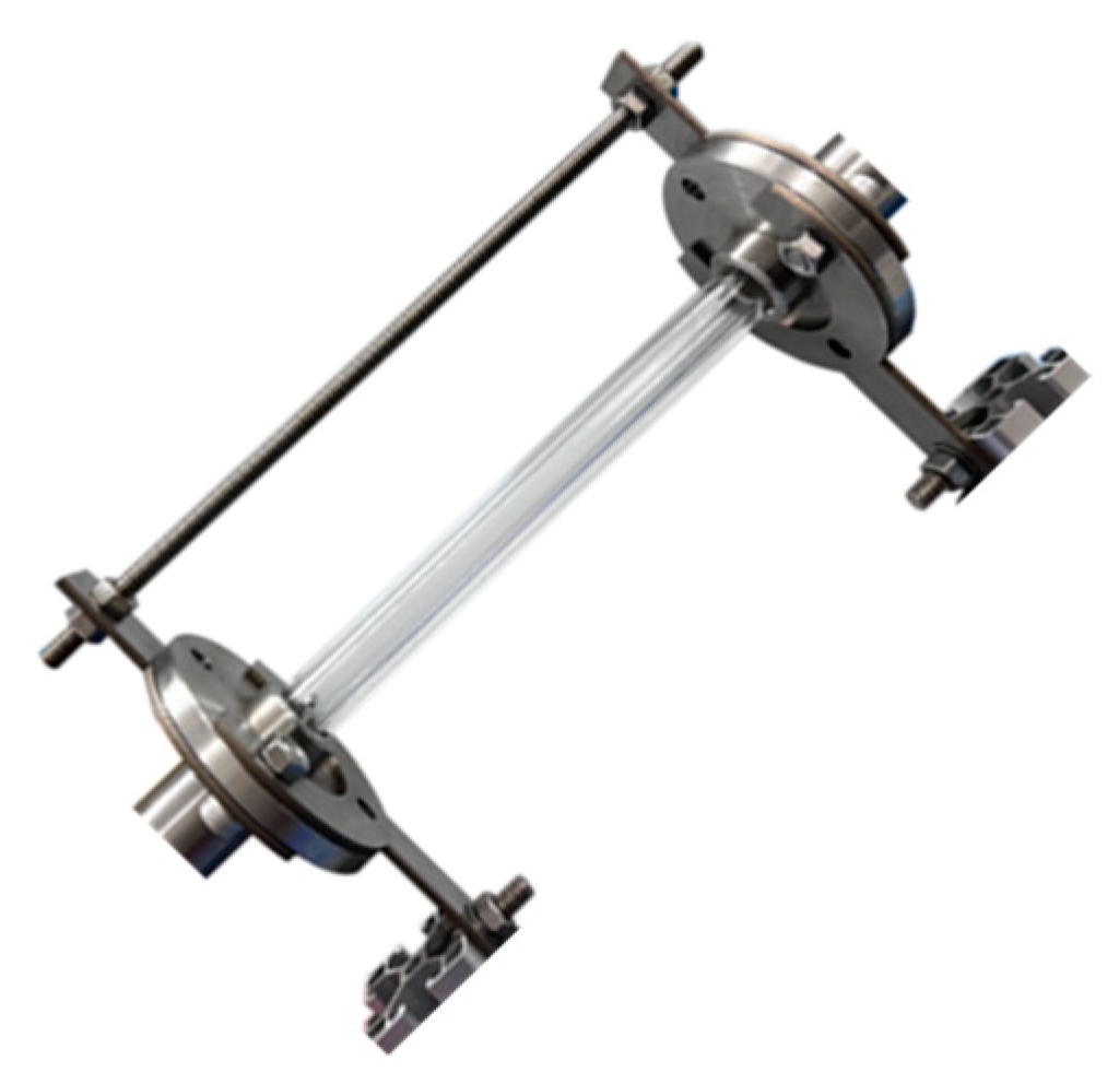
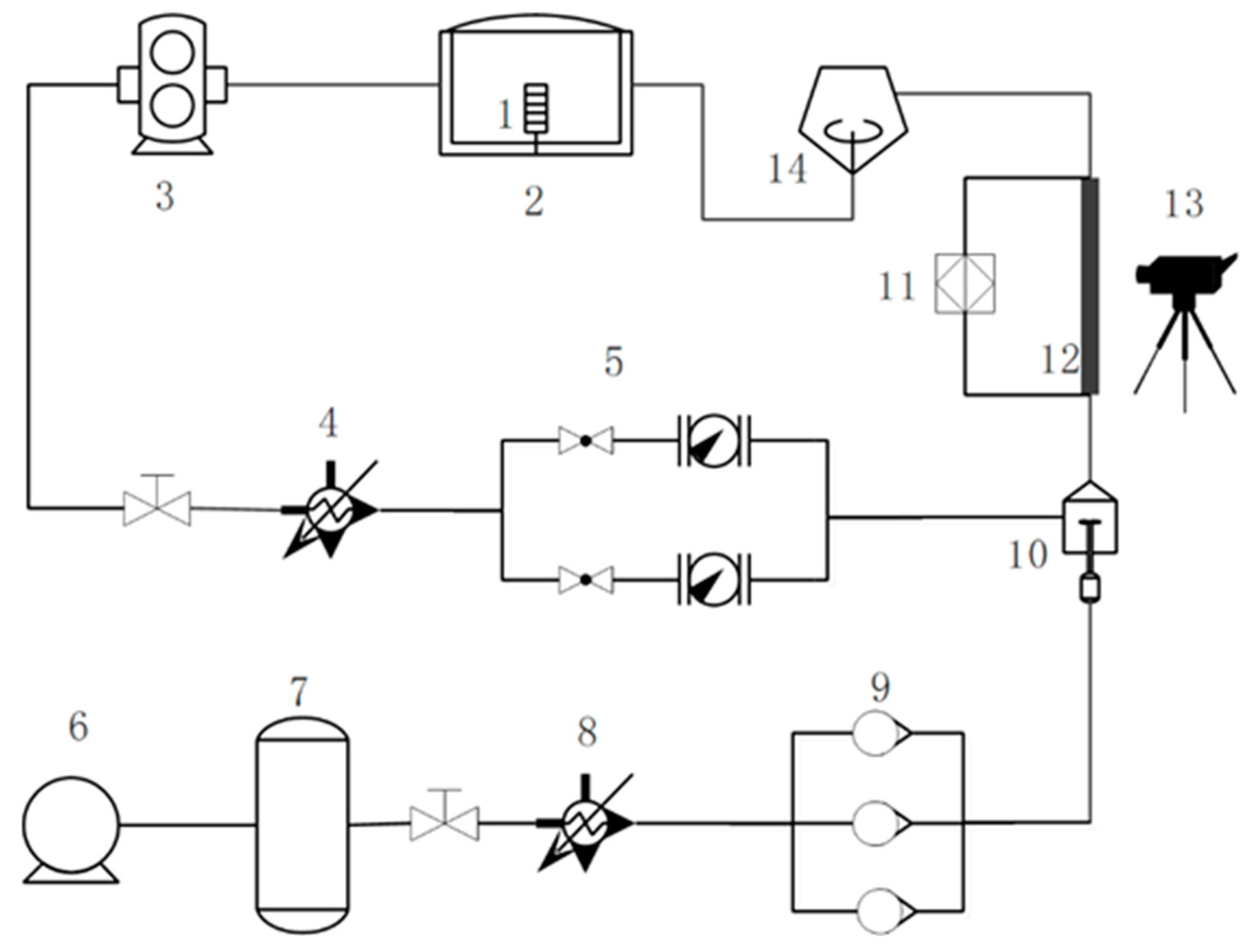
2. Visualization Test System

The model utilized for testing in this paper is illustrated in Figure 1. The pipe measures 10 mm in diameter, with 200 mm in length. The medium parameters are shown in

Table 1. Medium parameters.

Physical Properties	Air	Oil
ρ (kg/s)	0.954	1003.5
µ (kg/m·s)	2.18 × 10−5	0.0051
Cp (J/kg·K)	1.009 × 103	1880
λ (W/m·K)	0.0315	0.12

, and the temperature of the two-phase mixing is set to 370 K. The visualization pipe is placed at an inclination of 45 degrees, and a high-speed camera is employed to record the visualization segment of the test. The frame rate of the capture is 5000 fps.

Where ${\omega }_l, {\omega }_g$ denotes the liquid and gas phase reduced speed, respectively, defined as:

$${\omega }_l={\displaystyle \frac{V_l}{A}},$$

(1)

$${\omega }_g={\displaystyle \frac{V_g}{A}},$$

(2)

where: $V_l, V_g$ is the volume flow rate of the liquid and gas phases, respectively; A is the cross-sectional area of the flow channel.

The visualization test system diagram of the inclined pipe of the return oil pipeline is shown in Figure 2 and Figure 3. The experimental system is mainly divided into an oil circuit, a gas circuit, and a mixing pipe. The medium of the gas circuit is air, which is compressed by a compressor into a pressure stabilization tank, allowing for a continuous and stable supply of gas. A gas heater is used to heat the gas, and the supply flow rate of the gas line is regulated by a gas mass flow controller so that the gas meets the target parameter requirements before entering the mixer. The oil line is supplied from a tank via an oil pump, which is a heatable oil tank to raise the base temperature of the sliding oil. The flow rate of the oil circuit is adjusted using a liquid flow controller, and then the oil enters the oil heater to change the oil before entering the mixer to meet the target parameters. The oil and gas lines are uniformly mixed through the gas-liquid mixer and then enter the visualization test tube, where the flow directions are bottom-up and top-down, respectively. Temperature monitoring points are positioned at both extremities of the clear observation tube, constructed from robust quartz glass for visualization purposes, allowing the flow inside the tube to be captured by a high-speed camera. The mixed fluid flows out of the visualization tube into the gas-liquid separation device, through which the gas is discharged, and the gas-free oil flows into the tank along the pipeline, forming a cycle in the whole test system.

3. Results

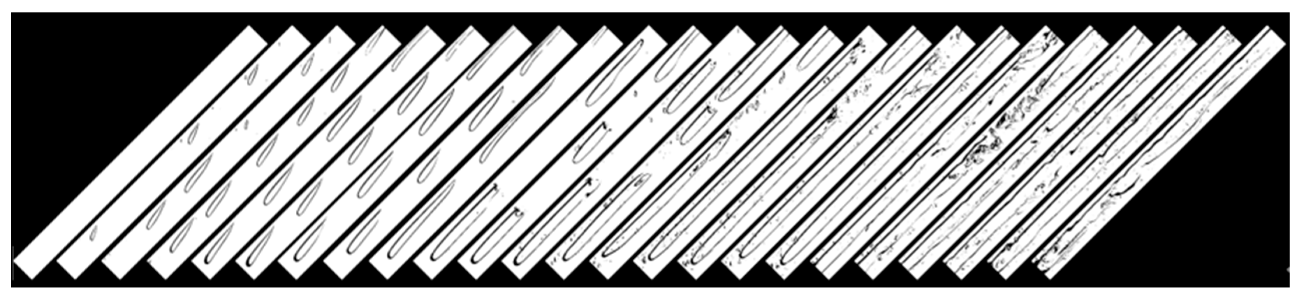
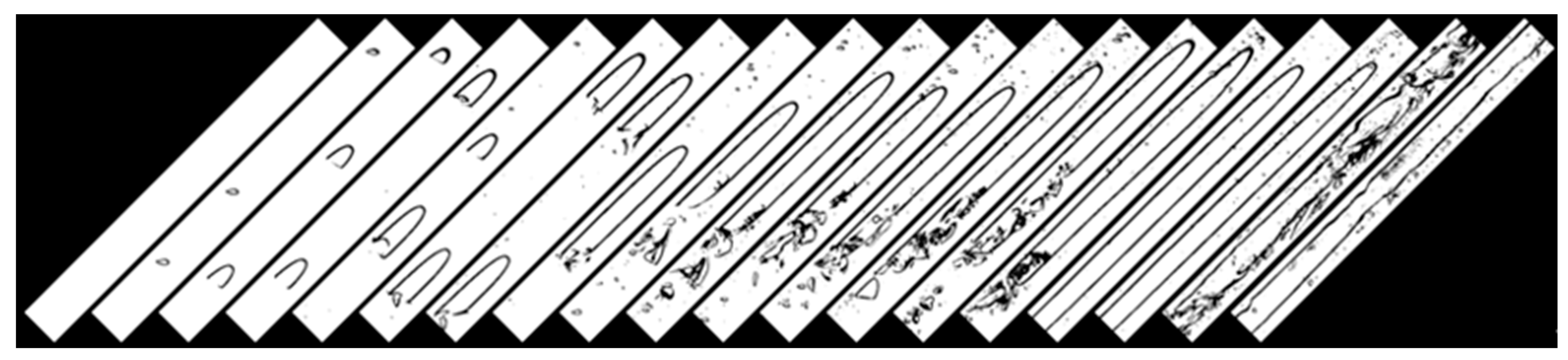
3.1. Experimental Study of Two-Phase Flow of Oil and Gas in Scavenge Pipe

The experimental setup for visualizing the oil-gas flow in a scavenge pipe is established, as shown in Figure 1. The visualized test section has a diameter of 10 mm and a length of 200 mm. The pipeline is placed at a 45-degree angle, and the intended temperature of the gas-liquid medium after mixing is 370 K. The flow direction is from bottom to top and from top to bottom, respectively. By using a high-speed camera to capture the flow changes inside the tube, the flow situation inside the tube can be obtained as the inlet gas increases at different liquid phase conversion speeds. Simple binarization processing can be performed on the captured images to analyze the flow situation inside the tube more effectively.

The flow direction is from top to bottom when the liquid phase reduces speed ${\omega }_l=0.378 \mathrm{m}/\mathrm{s}$. The flow situation of oil and gas two-phase flow in the visualization test pipeline is illustrated in Figure 4. With the increase in the gas-phase reduced speed, the bubbles in the pipe gradually grow into various flow patterns. The gas-phase reduced speed in the pipe changes in 0~2.12 m/s. Bubble flow occurs when the air intake is small, the bubble head is hemispherical, and the tail is pointed under gravity due to the tilted pipeline and downward flow of fluids. Under the influence of gravity, the head of the bubble is hemispherical, and the tail is pointed. As the inlet volume increases further, the bubble becomes longer due to the restriction of the pipe wall. At the gas-phase reduced speed of 0.212 m/s, the end of the bubble is flat, and there are some tiny bubbles at the back of the end. As the gas-phase discount velocity increases to 1.27 m/s, an annular flow is formed in the tube, and the liquid film on the upper wall is thinner than that on the lower wall. As shown in Figure 5 for the gas-phase conversion speeds of 0.085, 0.127, 0.212 m/s, respectively, with the liquid-phase conversion speed increasing the morphology of bubbles in the tube, the liquid-phase conversion speed changes in the range of 0.233 to 0.502 m/s. The figure shows that with the increase in the amount of oil feed, the bubbles are extruded, and the number of them changes to a small number of smaller and smaller morphology.

When the liquid-phase reduced speed ${\omega }_l=0.386 \mathrm{m}/\mathrm{s}$, the flow direction is from the bottom upwards, and the flow of oil and gas two-phase flow in the visualization test pipe is shown in Figure 6, and the range of the gas-phase reduced speed in the pipe is 0~2.12 m/s. When the air inlet volume is small, it is a bubble flow, and upon the augmentation of inlet airflow, the tiny bubbles grow further and become more extensive. The pipe is placed at an angle, and the fluid flows upwards, affected by the flow direction and gravity. The bubblehead is hemispherical, and the tail is flat, which is not quite the same as the downward-flowing bubbles in the pipe. The bubbles gradually elongate with the further increase in the inlet airflow and the restriction of the tube wall surface. In the gas-phase reduced speed of 1.148 m/s, the final formation is annular flow; the liquid film on the upper wall is thinner than the lower wall. As shown in Figure 7, the morphology of the bubbles in the tube increases with the liquid-phase reduced speed when the gas-phase reduced speed is 0.085, 0.127, and 0.212 m/s, respectively, and the liquid-phase reduced speed varies in the range of 0.149 to 0.623 m/s. It can be found in the figure that the bubbles in the tube are compressed significantly with the increase in the inlet oil volume, and the bubbles are compressed into smaller sizes and smaller volumes.

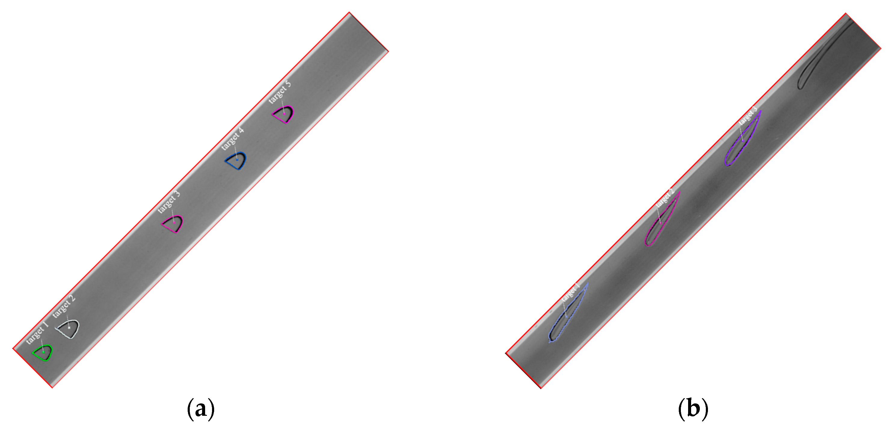
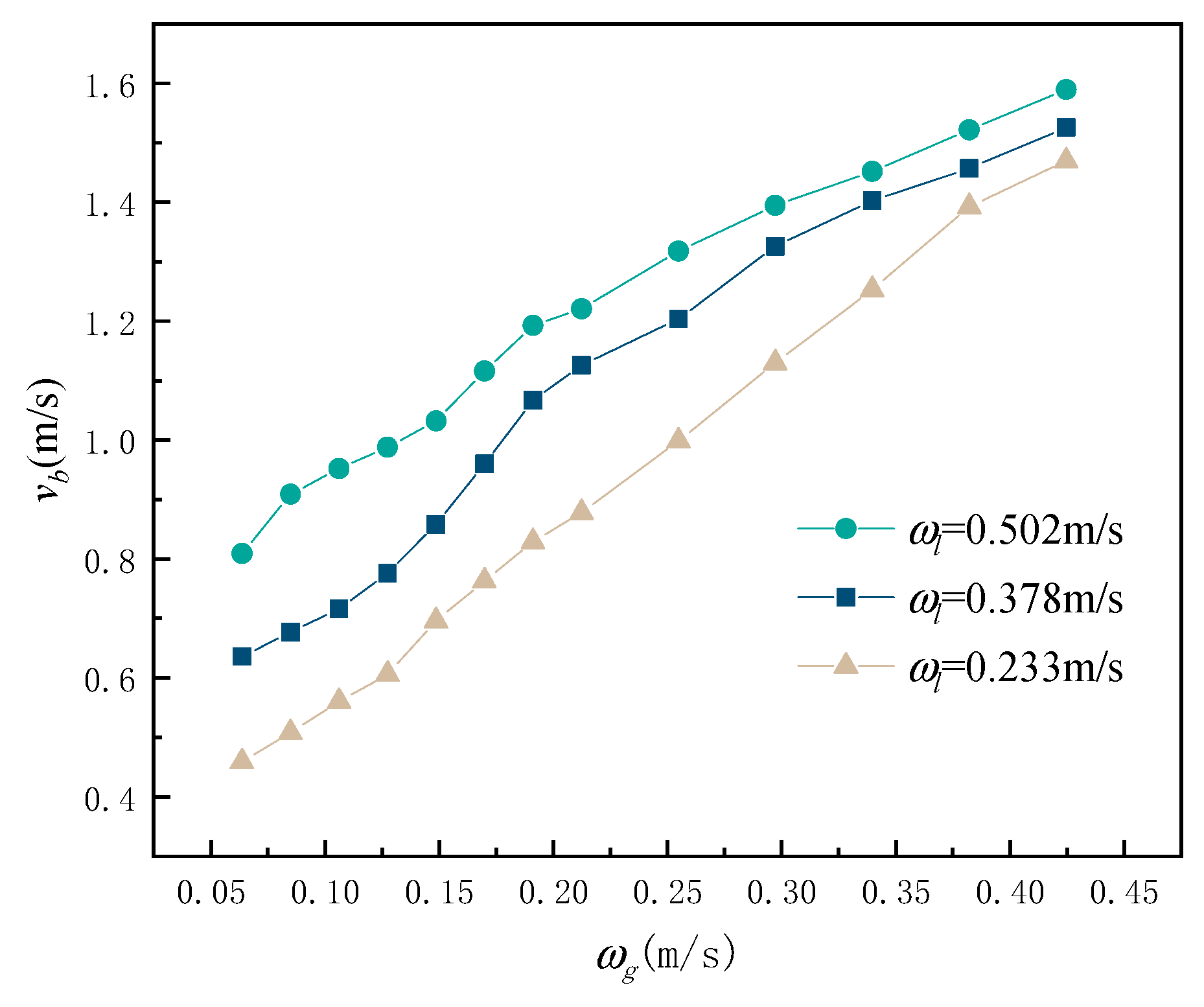
3.2. Analysis of Bubble Movement in Oil-Gas Two-Phase Flow Pipe

The inclined scavenge pipe is visualized, and the visualized pipe is photographed using a high-speed camera to obtain a clear picture of the bubble movement patterns inside the pipe. The frame rate of the photographed image is 5000 fps, and software is set up to analyze the movement parameters of the bubbles inside the target picture. As shown in Figure 8, the software is used to analyze the motion of bubbles in the target picture; using the grayscale value of the photograph reading for target identification, the size of the read picture is calibrated, the frame rate of the shooting is set as a time scale, and the changes of adjacent target pictures are compared and analyzed. The motion parameters of the target bubbles are obtained in the end.

As shown in Figure 9, the apparent velocity change of bubbles in the tube flowing from top to bottom is shown. When the liquid-phase commutation velocity is kept constant, the apparent velocity of the bubbles gradually increases with the increase in the gas-phase commutation velocity, and the growth rate of their bubble velocity is first fast and then slow. The turning point of the bubble’s apparent velocity growth is located at the gas-phase reduced speed of 0.212 m/s; due to the effect of gravity on the flow of bubbles in the tube in different flow directions, the growth rate of the bubble velocity in the tube is more significant in the top-down flow.

As shown in Figure 10, the change in apparent velocity of bubbles in the tube flowing from the bottom up is shown. From the change curve in the figure, the apparent velocity of the bubbles increases gradually with the gradual increase in the inlet volume when the oil-reduced velocity is constant. When the gas-reduced speed is less than 0.255 m/s, the growth rate of the apparent velocity of bubbles is more significant with the increase in the gas-reduced speed; after the gas-reduced speed is greater than the critical value of 0.255 m/s, the apparent velocity of bubbles slows down with the change in the gas-phase conversion speed. The increase in the apparent velocity of the bubbles is slowed down because the flow resistance increases further with the rise in the flow velocity of the gas and liquid phases.

3.3. Establishing a Prediction Model for Bubble Flow inside a Pipe

In machine learning, data regression prediction is a common supervised learning task. Data regression prediction aims to find a relationship between input features and output labels and build a function or model to describe this relationship. This function is usually a continuous mapping, so the model can be used to predict its corresponding continuous numerical output when new input data are available. In machine learning, there are various models for making data regression predictions. This paper uses four algorithms, namely, BP neural networks, radial basis neural networks, random forests, and support vector machines, for model building.

A BP neural network, or backpropagation neural network, is a standard artificial neural network model widely used in machine learning and pattern recognition. This network model consists of neurons connected through multiple layers, where each layer is connected to the next, the signals are transmitted, and the output is computed through weights. A radial basis neural network is a three-layer forward network with a vital mapping function, and its principle is closer to the backpropagation neural network; the essential feature is to use the radial basis function as the hidden layer activation function. The data from the input layer are entered into the hidden layer through the radial basis function of the nonlinear mapping and then passed to the output layer for output after linear calculation. Random forest is a classical integrated learning method commonly used for classification and regression problems. It consists of multiple decision trees and synthesizes the results of each decision tree by voting or averaging. A support vector machine is a supervised learning algorithm widely used in pattern recognition and machine learning. The main idea of the support vector machine is to find an optimal hyperplane that separates samples of different classes. A hyperplane can be understood as an N − 1 dimensional space, where N is the feature dimension of the samples. For binary classification problems, the hyperplane can separate the data into two classes. For multicategorization problems, multiple binary classifiers can be constructed using a one-to-many or one-to-one strategy.

This paper establishes a prediction model for the flow characteristics of bubbles in a tube. The target parameter of the prediction model is the apparent flow velocity of the bubbles in the tube, and the three characteristic parameters for selecting the input parameters are the radian value of the angle of the flow direction of the test tube, the reduced speed of the gas phase, and the reduced speed of the liquid phase. The angle of the flow direction of the test tube is obtained by taking the positive direction of the x-axis as the starting point. Four algorithms, BP neural network, radial basis neural network, random forest, and support vector machine, were used sequentially for data regression prediction modeling.

The training set comprised 100 data points, and 30 test samples were used to select the model. The root mean square error and coefficient of determination under the four algorithmic prediction models are shown in

Table 2. Indicators for the assessment of data regression models.

Data Regression Prediction Model	RMSE	R2
BP Neural Network	0.022059	0.97367
Radial Basis Function Neural Network	0.042145	0.98577
Random Forest	0.13949	0.81611
Support Vector Machine	0.030966	0.99572

as the evaluation metrics of the regression model. RMSE (Root Mean Square Error) is a metric in the evaluation of the regression model, which measures the prediction error of the model. R² (R-squared) is called the coefficient of determination, which is used as a measure of the degree of the model’s explanation of the variance of the data, i.e., the model’s goodness of fit to the observed data. From the table, it can be seen that the three algorithms, BP neural network, radial basis neural network, and support vector machine, have lower Root Mean Square Error (RMSE) and, at the same time, have better Coefficient of Determination (CoD). The BP neural network algorithm has the lowest RMSE for the prediction model, and the support vector machine algorithm has the highest CoD. The comparison of the test set prediction results of the two algorithms is shown in Figure 11. The data prediction model of the BP neural network algorithm has a lower error. Still, the prediction model of the support vector machine algorithm can fit the data very well, and its error is less than 5%, which can better predict the flow characteristics of the bubbles in the tube better. Combining machine learning and bubble flow analysis in the tube to establish a variety of prediction models, a comparative study of the BP neural network algorithm and support vector machine algorithm shows that the two algorithms can establish an objective and accurate prediction model. The model established in this paper can truthfully and precisely predict the bubble flow in the tube and contribute to the study of oil-gas flow in the scavenge pipe.

4. Conclusions

This paper establishes a visual pipeline test bed with the scavenge pipe tilted at 45 degrees; the flow directions are upward and downward, respectively, and the test temperature is 370 K. A high-speed camera photographs three main flow types, bubble, elastic, and annular flow, to obtain the effects of oil-gas reduced velocities on the change in bubble flow state in the pipe. The bubbles are extruded with the increase in the amount of oil feed, and the number changes to a small number of smaller and smaller morphology.

Based on high-speed photography, we establish the bubble flow characteristics of the tube flow analysis software, to obtain, respectively, the upward and downward flow of the apparent velocity of the bubble changes in the tilted 45-degree tube to explore the effect of gas-phase velocity and liquid-phase conversion velocity on the apparent velocity of the bubble in the tube. Due to the effect of gravity on the flow of bubbles in the tube in different flow directions, the growth rate of the bubble velocity is more significant in the top-down flow.

This paper establishes a regression prediction model for the apparent velocity of air bubbles in tubes and carries out prediction and evaluation. The root mean square error of the prediction model of the BP neural network algorithm is as low as 0.022059, and the coefficient of determination of the prediction model of the support vector machine algorithm is as high as 0.99572. A combination of the BP neural network algorithm and support vector machine algorithm can truthfully and precisely predict bubble flow in the tube to achieve the expected goal of the prediction model.

References

1. Li, G.Q. Present and future of aeroengine oil system. Aeroengine 2011, 6, 49–52. [Google Scholar]
2. Peng, Q.; Guo, Y.-Q.; Sun, H. Modeling and Fault Diagnosis of Aero-engine Lubricating Oil System. In Proceedings of the 2018 37th Chinese Control Conference (CCC), Wuhan, China, 25–27 July 2018; pp. 5907–5912. [Google Scholar] [CrossRef]
3. Chandra, B.; Simmons, K.; Pickering, S.; Collicott, S.H.; Wiedemann, N. Study of gas/liquid behavior within an aero enginebearing chamber. J. Eng. Gas Turbines Power 2013, 135, 051201. [Google Scholar] [CrossRef]
4. Flouros, M.; Iatrou, G.; Yakinthos, K.; Cottier, F.; Hirschmann, M. Two-Phase Flow Heat Transfer and Pressure Drop in Horizontal Scavenge Pipes in an Aero-engine. J. Eng. Gas Turbines Power 2015, 137, 081901. [Google Scholar] [CrossRef]
5. Mandhane, J.; Gregory, G.; Aziz, K. A flow pattern map for gas—Liquid flow in horizontal pipes. Int. J. Multiph. Flow 1974, 1, 537–553. [Google Scholar] [CrossRef]
6. Hibiki, T.; Mishima, K. Flow regime transition criteria for upward two-phase flow in vertical narrow rectangular channels. Nucl. Eng. Des. 2001, 203, 117–131. [Google Scholar] [CrossRef]
7. Mesa, D.; Quintanilla, P.; Reyes, F. Bubble Analyser-An open-source software for bubble size measurement using image analysis. Miner. Eng. 2022, 180, 107497. [Google Scholar] [CrossRef]
8. Thaker, J.; Banerjee, J. Characterization of two-phase slug flow sub-regimes using flow visualization. J. Pet. Sci. Eng. 2015, 135, 561–576. [Google Scholar] [CrossRef]
9. Rafałko, G.; Mosdorf, R.; Górski, G. Two-phase flow pattern identification in minichannels using image correlation analysis. Int. Commun. Heat Mass Transf. 2020, 113, 104508. [Google Scholar] [CrossRef]
10. Dong, F.; Zhang, S.; Shi, X.; Wu, H.; Tan, C. Flow Regimes Identification-based Multidomain Features for Gas–Liquid Two-Phase Flow in Horizontal Pipe. IEEE Trans. Instrum. Meas. 2021, 70, 1–11. [Google Scholar] [CrossRef]
11. De Giorgi, M.G.; Ficarella, A.; Lay-Ekuakille, A. Monitoring Cavitation Regime From Pressure and Optical Sensors: Comparing Methods Using Wavelet Decomposition for Signal Processing. IEEE Sensors J. 2015, 15, 4684–4691. [Google Scholar] [CrossRef]
12. Ji, H.; Long, J.; Fu, Y.; Huang, Z.; Wang, B.; Li, H. Flow Pattern Identification Based on EMD and LS-SVM for Gas–Liquid Two-Phase Flow in a Minichannel. IEEE Trans. Instrum. Meas. 2011, 60, 1917–1924. [Google Scholar]
13. Liang, X.; Wang, S.; Shen, W. Random Forest Model of Flow Pattern Identification in Scavenge Pipe Based on EEMD and Hilbert Transform. Energies 2023, 16, 6084. [Google Scholar] [CrossRef]
14. Chen, R.-C.; Dewi, C.; Huang, S.-W.; Caraka, R.E. Selecting critical features for data classification based on machine learning methods. J. Big Data 2020, 7, 52. [Google Scholar] [CrossRef]
15. Bacu, V.; Nandra, C.; Sabou, A.; Stefanut, T.; Gorgan, D. Assessment of Asteroid Classification Using Deep Convolutional Neural Networks. Aerospace 2023, 10, 752. [Google Scholar] [CrossRef]
16. Yang, L.; Jia, G.; Zheng, K.; Wei, F.; Pan, X.; Chang, W.; Zhou, S. An Unmanned Aerial Vehicle Troubleshooting Mode Selection Method Based on SIF-SVM with Fault Phenomena Text Record. Aerospace 2021, 8, 347. [Google Scholar] [CrossRef]
17. Chandra, M.A.; Bedi, S.S. Survey on SVM and their application in imageclassification. Int. J. Inf. Technol. 2021, 13, 1–11. [Google Scholar]
18. Moura, M.d.C.; Zio, E.; Lins, I.D.; Droguett, E. Failure and reliability prediction by support vector machines regression of time series data. Reliab. Eng. Syst. Saf. 2011, 96, 1527–1534. [Google Scholar] [CrossRef]
19. Steyerberg, E.W.; van der Ploeg, T.; Van Calster, B. Risk prediction with machine learning and regression methods. Biom. J. 2014, 56, 601–606. [Google Scholar] [CrossRef] [PubMed]
20. Wu, Y.-C.; Feng, J.-W. Development and application of artificial neural network. Wirel. Pers. Commun. 2018, 102, 1645–1656. [Google Scholar] [CrossRef]
21. Kawahara, A.; Sadatomi, M.; Nei, K.; Matsuo, H. Experimental study on bubble velocity, void fraction and pressure drop for gas–liquid two-phase flow in a circular microchannel. Int. J. Heat Fluid Flow 2009, 30, 831–841. [Google Scholar] [CrossRef]
Figure 1. Visual test pipeline tilted at 45°.
Aerospace 11 00655 g001
Figure 2. Visual test system diagram for scavenge pipe. 1. Oil heater; 2. Fuel tank; 3. Oil pump; 4. Lubricating oil heater; 5. Turbine flow meter; 6. Air pump; 7. Pressure stabilizing tank; 8. Gas heater; 9. High-quality flow controller; 10. Gas-liquid mixer; 11. Thermocouples; 12. Visualization pipelines; 13. High-speed camera; 14. Gas-liquid separator.
Aerospace 11 00655 g002
Figure 3. Test bench.
Aerospace 11 00655 g003
Figure 4. When flowing from top to bottom and ω l = 0.378   m / s , the flow inside the tube changes as the gas-phase reduced speed increases.
Aerospace 11 00655 g004
Figure 5. Changes in in-tube flow with increasing liquid-phase reduced speed in top-down flow. (a) ω g = 0.085   m / s . (b) ω g = 0.127   m / s . (c) ω g = 0.212   m / s .
Aerospace 11 00655 g005
Figure 6. When flowing from bottom to top and ω l = 0.386   m / s , the flow inside the pipe changes as the intake volume increases.
Aerospace 11 00655 g006
Figure 7. Changes in in-tube flow with increasing liquid-phase reduced speed in bottom-up flow. (a) ω g = 0.085   m / s . (b) ω g = 0.127   m / s . (c) ω g = 0.212   m / s .
Aerospace 11 00655 g007
Figure 8. Target recognition map for taking photographs. (a) Bottom-up. (b) Top-down.
Aerospace 11 00655 g008
Figure 9. Flow direction is upward, and the bubble flow rate inside the tube varies with inlet velocity.
Aerospace 11 00655 g009
Figure 10. Flow direction is downward, and the bubble flow rate inside the tube varies with inlet velocity.
Aerospace 11 00655 g010
Figure 11. Comparison of test set predictions for data regression prediction models. (a) BP neural network model. (b) Support vector machine model.
Aerospace 11 00655 g011