Decoys Deployment for Missile Interception: A Multi-Agent Reinforcement Learning Approach

Abstract

Recent advances in radar seeker technologies have considerably improved missile precision and efficacy during target interception. This is especially concerning in the arenas of protection and safety, where appropriate countermeasures against enemy missiles are required to ensure the protection of naval facilities. In this study, we present a reinforcement-learning-based strategy for deploying decoys to enhance the survival probability of a target ship against a missile threat. Our approach involves the coordinated operation of three decoys, trained using the Multi-Agent Deep Deterministic Policy Gradient (MADDPG) and Multi-Agent Twin Delayed Deep Deterministic Policy Gradient (MATD3) algorithms. The decoys operate in a leader–follower dynamic with a circular formation to ensure effective coordination. We evaluate the strategy across various parameters, including decoy deployment regions, missile launch directions, maximum decoy speeds, and missile speeds. The results indicate that, decoys trained with the MATD3 algorithm demonstrate superior performance compared to those trained with the MADDPG algorithm. Insights suggest that our decoy deployment strategy, particularly when utilizing MATD3-trained decoys, significantly enhances defensive measures against missile threats.

1. Introduction

Advanced missile systems equipped with cutting-edge radar seeker technology pose a serious threat to naval platforms, which often suffer from limited manoeuvrability. In order to protect these platforms during adverse situations, defence tactics have evolved into two main approaches. While the soft-kill option concentrates on deceiving and distracting incoming threats, the hard-kill option seeks to physically eliminate detected threats. Decoys, which are a form of Electronic Countermeasure (ECM) technology, are frequently employed in soft-kill tactics to deceive radar seekers that direct missiles in their final stage. The success of a decoy mission is strongly dependent on important criteria such as deployment angle and time. A comprehensive investigation has been carried out to formulate effective tactics for decoying. However, it is essential to consistently develop new tactics for deceiving radar seeker technology in order to successfully challenge its current improvements.

1.1. Related Works

This paper [1] examines the developing difficulties encountered in protecting airborne platforms from Radio Frequency (RF) seeker-guided missile systems. The central focus is on assessing the effectiveness of off-board RF ECM techniques, with particular attention given to off-board ECM, in ensuring protection. Various operational factors essential for the efficient deployment of towed decoys are explored in [2], including the strength of reflection, tether length, and release direction. The research findings indicate that towed decoys can serve as effective countermeasures against monopulse seeker missiles, provided that optimal operational conditions are achieved. The working mechanism of Towed Radar Active Decoy (TRAD) is briefly introduced in [3], followed by an analysis of its importance in mitigating the threat posed by monopulse radar seekers in both ground-to-air and air-to-air combat situations. The outcomes of the study have determined that when the TRAD is equipped with a fixed cable length of 130 metres and the jamming power exceeds 45 dBmW, it effectively deflects radar seekers approaching from angles between 13 degrees and 163 degrees.

Modern naval forces face a serious threat from radar-guided anti-ship missiles, and ref. [4] makes the case for the use of off-board decoys as a tactical defensive measure. In order to maximise the protection offered by these decoys, this paper underscores the significance of deployment timing, deployment direction, and RF attributes of decoys. Ref. [5] presents an outline of utilising the “soft kill” tactic to divert sea-skimming missiles aimed at valuable assets like ships. The efficacy of strategically positioning an active decoy, launched from the target platform, is assessed in a simulation environment. The study suggests that increasing the jammer’s power can result in longer miss distances. The ECM and Electronic Counter-Countermeasures (ECCM) are perpetually engaged in a competitive dynamic, continually devising novel strategies to surpass each other. A comparative analysis is provided in [6] on the functionality of ECM and ECCM in hostile environments. While ECM focuses on improving the defensive capabilities of aircraft, ECCM strengthens ground-based radar systems. In [7], the role of a solitary decoy in aiding the evasion tactics of the evader is investigated through mathematical formulation that considers factors such as the decoy launch angle and timing of decoy deployment. Following this, the paper conducts extensive simulation analyses and observes a close correspondence between the analytical predictions and the simulation findings. This is accomplished through the examination of outcomes for diverse decoy launch angles and deployment timings.

A numerical simulator is developed in [8] to model radar echo signals in real-world scenarios in which an Expendable Active Decoy (EAD) and an airborne target are both in motion. Monte Carlo simulations are utilised to evaluate how different EAD parameters and deployment scenarios affect the probability of missing the target. The study [9] explores the suitability of mobile decoys in marine and underwater environments to assess their efficacy in employing deceptive tactics aimed at diverting the incoming interceptor from its intended trajectory. These decoys have the ability to mimic the acoustic signature of the target and transmit it to the interceptor. This paper [10] develops a simulation and modelling method aimed at assessing the jamming effectiveness of a repeater-type active decoy against a ground-tracking radar in dynamic combat scenarios. The study centers on assessing time-domain echo signals and performing numerical simulations to analyze the coverage of jamming. Numerical findings demonstrate that circular polarization offers a more consistent jamming effectiveness when compared to linear polarization. A deep Q-learning-based approach is applied in [11] to guide a false target for the protection of a true target against high mobility threats in a land defence application. The findings indicate that employing the Q-learning-based method can effectively redirect threats approaching from various angles of approach, even when the amount of training data is restricted.

The study [12] investigates how the RF characteristics of the active decoy, including antenna pattern and power amplifier gain, affect its jamming performance. It evaluates the effective jamming coverage in various engagement scenarios to evaluate the survivability of the airborne platform against RF threats. A scenario-driven simulation is created in [13] to evaluate how well passive decoy systems can counter sea-skimming anti-ship missiles (ASMs). This simulation can model various features of the target ship, such as its radar cross-section (RCS) and evasive manoeuvres. The findings illustrate the impact of changes in input parameters, such as RCS and the directions from which decoys are launched, on the performance of the decoy system. This study [14] explores the most effective trajectory patterns for a swim-out acoustic decoy designed to counter acoustic homing torpedoes. It examines various factors impacting the effectiveness of these countermeasures. The authors then employ a genetic algorithm to determine the optimal trajectory parameters for different scenarios based on a predefined assessment criterion. The simulation results show that straight line, second turn-angle, and snake trajectories are better at keeping acoustic-homing torpedoes away from the target submarine than helical and circular trajectories.

The paper [15] emphasises the importance of utilising modelling and simulation (M&S) engineering as a valuable tool in designing and evaluating underwater warfare systems, particularly in addressing challenges related to countering torpedo attacks. The anti-torpedo simulator features both decoys as countermeasures and a simple jammer. Despite the simplicity of the jammer, it is argued that it aids in understanding how different jammer configurations impact the effectiveness of anti-torpedo countermeasures. This paper [16] centers on optimizing the strategy for a submarine to countermeasure acoustic homing torpedoes using two swim-out acoustic decoys. The paper seeks to find the most effective countermeasure strategy by using a genetic algorithm and considering various factors, including decoy fire time, decoy turn angles, and decoy speeds. The problem of enhancing ship survivability against adversary torpedoes through the employment of both single and multiple decoy placements is addressed in [17]. The research compares several deployment strategies, including same-side and zig-zag deployment, and the findings indicate that zig-zag deployment surpasses same-side deployment in effectiveness.

The development and testing of a drone swarm configuration designed to obscure a flying target drone from ground-based radar detection are examined in [18]. The research examined four distinct configurations for drone swarms and concluded that Drone Swarm Architecture 4, utilizing multiple multirotor platforms, was the most efficient in terms of electromagnetic concealment and hover ability, despite certain drawbacks related to payload capacity and endurance. An approach employing mixed-integer linear programming (MILP) is suggested for allocating tasks to protect stationary surface assets through the use of decoys in [19]. The objective of this approach is to minimize the worst-case response time of the decoys to the threats, ensuring effective protection of assets against incoming threats. Additionally, the study examines the impact of burn-through range on the efficacy of decoys in protecting assets from incoming threats. A ducted-fan flight array system is proposed in [20] to carry out the decoy mission against ASMs. Each module is equipped with a conventional ducted-fan configuration and can fly independently. The study outlined in reference [21] examines task allocation for multiple UAVs acting as decoys to enhance the defense of a friendly ship against anti-ship missiles. The paper proposes an auction algorithm for task assignment, selected for its faster computational speed relative to alternative optimization methods.

These kinds of defence scenarios can be considered event-triggered because once a naval platform detects an approaching threat, a command is sent to activate the decoys. In [22], a cooperative formation approach is proposed for deploying USV-UAV platforms in maritime missions. The multi-decoy systems mentioned above struggle with making individual decisions based on their local information. In our research, we place a strong emphasis on the independent decision-making process through the use of reinforcement learning.

1.2. Contribution and Structure of the Paper

The primary contributions of this research are as follows: (1) To address the protection of the naval platform against missile threat, an AI-based decoy deployment strategy is proposed. For this purpose, we trained decoys through MADDPG and MATD3 algorithms and compared their impact on the mission success rate. (2) To assess the influence of the decoy deployment angle on mission success, we partitioned a full circle into six equal regions. The coordinated movement of decoys serves to elevate their collective RCS level, thereby ensuring mission success. We advocate for the adoption of a circular formation configuration, wherein one decoy is designated as the leader while the remainder act as followers. (3) We streamlined the reward function, assigning each decoy a singular contribution to the global reward. For the leader decoy, the reward sub-function incentives movement towards the assigned point, while for each follower decoy, the reward function is contingent upon adherence to the formation configuration.

The structure of this paper is outlined as follows: In Section 2, we define the problem addressed in this research and present the system modeling. Section 3 elaborates on the reinforcement learning algorithms employed in this study and discusses the enhancements introduced. Moving to Section 4, we introduce the developed simulation environment and outline the observation space, action space, and reward function used in our experiments. Following this, Section 5 details the simulation experiments conducted and provides an analysis of the experimental results obtained. Finally, in Section 6, we conclude the paper by summarizing the key findings and contributions of this research, along with suggestions for future work and potential applications of the proposed approach.

2. Problem Definition and Modelling

In this section, we first introduce the problem addressed in this paper, followed by a detailed description of the 2D kinematics model for the target ship, decoys, and missile threat.

2.1. Problem Definition

This paper examines a scenario in the marine environment in which an anti-ship missile targets a naval platform. As shown in Figure 1, when the situational awareness system detects a threat, a warning is given to activate multiple decoys in the appropriate direction to lure the approaching threat from the main platform. For this mission, it is planned to use a quadcopter with a jammer attached as a decoy.

This research assumes that the drone can easily carry the jammer payload without affecting its flight performance during the mission. Cooperative path planning is a crucial factor influencing the mission’s success. For this purpose, a leader-follower flight formation configuration is considered to be applied; one decoy is assigned as a leader, and the rest are followers. In situations where the distance between the target ship and the anti-ship missile is sufficiently large in electromagnetic terms, a scattering point referred to as a “scattering centre” may be utilised to represent the RCS of the target ship. Remarkably, during an engagement scenario, an ASM intercepts the virtual scattering centre rather than the actual target ship. Consequently, when the target ship releases a decoy with a specified RCS level in a direction away from itself, the scattering centre shifts along the line from the target to the decoy as visualized in Figure 2a. Consequently, the line of sight (LOS) changes, altering the susceptibility. The greater the RCS of the decoy, the farther the scattering centre moves from the target ship, thereby reducing its susceptibility to the ASM.

Inspired by the paper [13], we expand the formulation for multiple decoys to calculate the estimated value of the RCS level and position of the equivalent scattering centre (ESC).

$${\sigma }_{sc}=10{log}_{10}\left({10}^{{\sigma }_s/10}+{10}^{{\sigma }_{d1}/10}+\dots +{10}^{{\sigma }_{dn}/10}\right)$$

(1)

$$x_{sc}={\displaystyle \frac{{10}^{{\sigma }_s/10}{x}_s+{10}^{{\sigma }_{d1}/10}{x}_{d1}+\dots +{10}^{{\sigma }_{dn}/10}{x}_{dn}}{{10}^{{\sigma }_{sc}/10}}}$$

(2)

$$y_{sc}={\displaystyle \frac{{10}^{{\sigma }_s/10}{y}_s+{10}^{{\sigma }_{d1}/10}{y}_{d1}+\dots +{10}^{{\sigma }_{dn}/10}{y}_{dn}}{{10}^{{\sigma }_{sc}/10}}}$$

(3)

where sub $d\left[i\right]$ represents each single decoy, and $i=1,2,\dots n$ n is equal to 3 because the number of agents is 3 in this research. The ${\sigma }_s$, ${\sigma }_{d\left[i\right]}$, and ${\sigma }_{sc}$ are the RCS level in dBsm of the target ship, the RCS level of $\left[i\right]$th decoy, and the RCS level of the ESC point, respectively. The ($x_s$, $y_s$), ($x_{sc}$, $y_{sc}$), and ($x_{d\left[i\right]}$, $y_{d\left[i\right]}$) are the instantaneous position of the ship, the ESC point, and the $\left[i\right]$th decoy in meters, respectively.

The motivation for employing multiple decoys can be explained through two key points: Firstly, the effectiveness of a jammer’s signal power determines the payload size, thus, rather than employing a single large decoy with a heavy payload, utilizing multiple smaller decoys with lighter payloads can prove more efficient. Secondly, in the event of any decoy losses within a multi-decoy setup, the remaining decoys can continue executing the mission effectively.

2.2. Modelling

This section describes the 2D system model for the target ship, decoys, and missile threat, respectively.

2.2.1. Decoy Model

In a two-dimensional setting, there are N flying agents labelled with indices $i=1,2,\dots ,N$. One agent acts as the leader, whilst the other agents serve as followers. The positions and velocities of these agents are represented by $p_i$ and $v_i$, respectively. The dynamics of a each agent is modelled by

$$\begin{array}{cc}\hfill a_i^t& ={\displaystyle \frac{F_i^t}{m}}\hfill \\ \hfill v_i^t& =v_i^{t-1}+a_i^t\Delta t\hfill \\ \hfill p_i^t& =p_i^{t-1}+v_i^t\Delta t\hfill \end{array}$$

(4)

where $i=1,2,\dots N$, and $a_i^t,v_i^t,p_i^t\in {\mathbb{R}}^2$, denote the acceleration, velocity, and position of the agent i in time instance t, $\Delta t$ denotes the system sampling period; m is the mass of the agents, and $u_i^t=F_i^t\in {\mathbb{R}}^2$ defines the control force input of agent i.

2.2.2. Target Model

The kinematics equation for a point-mass model of the target ship is as follows

$$\begin{array}{cc}\hfill & {\dot{X}}_s=V_{s}cos{\phi }_s\hfill \\ \hfill & {\dot{Y}}_s=V_{s}sin{\phi }_s,\hfill \end{array}$$

(5)

where (${\dot{X}}_s$, ${\dot{Y}}_s$) are the Cartesian velocity coordinates of the ship, ${\phi }_s$ is the heading angle, and $V_s$ is the speed in the $(x,y)$ plane.

2.2.3. Missile Model

We use a point mass model to describe the anti-ship missile (ASM). The 2D kinematics equations that represent the ASM model is given by,

$$\begin{array}{cc}\hfill & {\dot{X}}_m=V_{m}cos{\phi }_m\hfill \\ \hfill & {\dot{Y}}_m=V_{m}sin{\phi }_m,\hfill \end{array}$$

(6)

where (${\dot{X}}_m$, ${\dot{Y}}_m$) are the linear velocities of the inertial frame, and $V_m$ and ${\phi }_m$ denote the velocity and heading angle of the ASM, respectively.

This paper focuses on a missile’s terminal guiding phase. As a result, it is assumed that the missile has information about its target, and the guiding law is applied following the missile’s preferred engagement mode. Figure 3 depicts the geometry of the missile engagement model. The terms $v_T$, $v_M$, $n_T$, and $n_V$ represent the target velocity, missile velocity, target acceleration, and missile lateral acceleration, respectively. From Figure 3 we can observe the following relation,

$$R_{TM}=\sqrt{(R_{TMe}^2+R_{TMn}^2)}$$

(7)

where $R_{TM}$ is the distance between the target and the missile during the engagement. The line-of-sight angle ($\lambda$) can be easily determined by,

$$\lambda =arctan\left({\displaystyle \frac{R_{TMe}}{R_{TMn}}}\right).$$

(8)

Additionally, the relative velocity of the target and the missile is determined separately for each axis by,

$$\begin{array}{cc}\hfill V_{TMe}& =V_{Te}-V_{Me},\hfill \end{array}$$

(9)

$$\begin{array}{cc}\hfill V_{TMn}& =V_{Tn}-V_{Mn}.\hfill \end{array}$$

(10)

If we take the time-derivative of (8) yields the line-of-sight rate given by,

$$\dot{\lambda }={\displaystyle \frac{R_{TMe}{V}_{TMn}-R_{TMn}{V}_{TMe}}{R_{TM}^2}}.$$

(11)

The closing velocity $V_c$ is defined as the negative rate of change of the missile-target range $R_{TM}$, which can be calculated as,

$$V_c={\displaystyle \frac{-(R_{TMe}{V}_{TMe}+R_{TMn}{V}_{TMn})}{R_{TM}}}.$$

(12)

Using the principles of proportional navigation guidance law, we can determine the magnitude of the missile guidance command $n_c$ as follows,

$$n_c=N{V}_c\dot{\lambda }.$$

(13)

3. Reinforcement Learning

3.1. Basic Concepts of Reinforcement Learning

Reinforcement Learning formalizes the interaction between an autonomous agent and its environment using a framework known as a Markov Decision Process (MDP) as indicated in the Figure 4. An MDP is characterized by a tuple $(S,A,R,T,\gamma )$, where S denotes a finite set of states, and A signifies a finite set of actions. The transition function $T:S\times A\times S\to [0,1]$ defines the probability of transitioning from a state $s\in S$ to another state $s^{\prime }\in S$ given a specific action $a\in A$. The reward function $R:S\times A\times S\to \mathbb{R}$ specifies the immediate reward, which may be stochastic, that the agent receives when it performs action a in state s and transitions to state $s^{\prime }$. The parameter $\gamma$ represents the discount factor, balancing the importance of immediate rewards versus future rewards.

In reinforcement learning, after an action is executed, a reward—either positive or negative—is provided as feedback to assess the action’s effectiveness. The cumulative reward at each time step t is calculated using the following formula:

$$R\left(\tau \right)=r_{t+1}+r_{t+2}+r_{t+3}+r_{t+4}+\dots .$$

(14)

However simply summing the rewards is not practically viable, so a discount factor is introduced into the equation. This discount factor adjusts future rewards by exponentially weighting them according to their time step, making them comparable to immediate rewards. Near-term rewards are more reliable as they are more predictable than those projected far into the future. The modified formula for computing cumulative rewards is given below:

$$R\left(\tau \right)=r_{t+1}+\gamma r_{t+2}+{\gamma }^2{r}_{t+3}+{\gamma }^3{r}_{t+4}+\dots .$$

(15)

this corresponds to:

$$R\left(\tau \right)=\sum _{n=1}^{\infty }{\gamma }^k{r}_{t+k+1}$$

(16)

The discount factor $\gamma$ (gamma) is a key parameter in reinforcement learning, ranging between 0 and 1. A higher $\gamma$ value implies less discounting of future rewards, encouraging the agent to focus on long-term gains. Conversely, a lower $\gamma$ results in greater discounting, prioritizing short-term rewards. An essential concept in reinforcement learning is the exploration/exploitation trade-off. Exploration involves experimenting with random actions to acquire new knowledge about the environment, whereas exploitation leverages existing knowledge to make optimal decisions. There are two main approaches to training reinforcement learning (RL) agents: policy-based and value-based methods. Policy-based methods directly learn a policy that guides the agent in selecting actions to maximize the cumulative expected return. In deterministic policies, a specific action is chosen for each state, while stochastic policies produce a probability distribution over possible actions for a given state. Value-based methods, on the other hand, rely on a value function, which maps each state to its expected value, helping to indirectly determine the optimal action. A common alternative to the value function is the action–value function, denoted as $Q(s,a)$, which provides a measure of the expected reward for taking a particular action in a given state. Q-learning is one of the most prominent techniques for computing Q-values, facilitating effective decision-making in RL agents.

3.2. Centralized Training Decentralised Execution (CTDE) Framework

Applying a single-agent reinforcement learning algorithm to train multiple agents is ineffective due to the non-stationary nature of transitions in such scenarios. In a Markov Decision Process (MDP), which is the framework used for single-agent reinforcement learning, it is assumed that the transition probabilities for each state-action pair remain constant over time. However, when multiple agents are trained in the same environment, this assumption no longer holds, as the actions of each agent can influence the environment and thus alter the transition dynamics for other agents.

Multi-Agent Reinforcement Learning (MARL) is a framework to train multi agents to collectively learn, collaborate, and interact with each other in the same environment. Two primary challenges faced by MARL algorithms are non-stationary transitions and exponentially expanding state and action spaces. As the number of agents increases, the sizes of both the state and action spaces grow exponentially, leading to the curse of dimensionality, which complicates the learning process. Various approaches [23,24] have been proposed to address these challenges. Most of them fall under the umbrella of a framework known as centralized training with decentralized execution.

Centralised training and decentralised execution (CTDE) [25] is an approach employed MARL that handles the computing complexity during the training phase versus during execution. An often used approach to implement this technique is the training of a centralised critic and the execution of decentralised actors, as shown in Figure 5. This method expands upon the policy-gradient actor–critic model. In this configuration, the critic network is trained in a non-real-time manner, without being limited by the need for immediate performance. The main goal is to make it possible for decentralised policies to be learned that can solve cooperative multi-agent tasks efficiently by utilising global information that is collected by multiple agents during training but not during task execution.

Multi-Agent Deep Deterministic Policy Gradient (MADDPG) [25] algorithm presents an actor-critic based solution for tackling multi-agent problems, drawing inspiration from its single-agent counterpart, Deep Deterministic Policy Gradient (DDPG) [26]. The core idea behind MADDPG is that if all agents’ actions are known, the environment remains stationary even as the policies change. The pseudocode for the MADDPG algorithm is provided in Algorithm 1. Similar to DDPG, MADDPG is an off-policy algorithm that utilizes random samples from a buffer of experiences accumulated during training. Each agent has its observation and continuous action space, along with four neural networks: actor, critic, target actor, and target critic. The actor network produces deterministic actions based on local observations, while the critic network evaluates the actor’s performance by computing the Q-value. Unlike typical policies that output probability distributions, the actor’s network directly maps state information to action results. The framework of centralized training with decentralized execution, as depicted in Figure 5, enables policies to leverage additional information for enhanced training. In this approach, the actor can only access local information, while the critic is enriched with data from other agents. Key parameters such as joint states, next joint states, joint actions, and rewards received by each agent are stored in an experience buffer at each step. During training, a batch of random samples from the experience replay buffer is utilized to train the agents.

Algorithm 1: Multi-Agent Deep Deterministic Policy Gradient for N agents [25]

$\mathbf{for}\mathrm{episode}=1\mathrm{to}\mathrm{M}\mathbf{do}$      $\mathrm{Initialize}\mathrm{a}\mathrm{random}\mathrm{process}\mathcal{N}\mathrm{for}\mathrm{action}\mathrm{exploration}$      $\mathrm{Receive}\mathrm{initial}\mathrm{state}\mathrm{x}$      $\mathbf{for}\mathrm{t}=1\mathrm{to}\mathrm{T}\mathbf{do}$        $\mathrm{for}\mathrm{each}\mathrm{agent}i,\mathrm{select}\mathrm{action}{a}_i$ = ${\mu }_{{\theta }_i}$$\left(o_i\right)+{\mathcal{N}}_t\mathrm{w}.\mathrm{r}.\mathrm{t}\mathrm{the}\mathrm{current}\mathrm{policy}\mathrm{and}\mathrm{exploration}$        $\mathrm{Execute}\mathrm{actions}a=\left(a_1,\dots ,a_N\right)\mathrm{and}\mathrm{observe}\mathrm{reward}r\mathrm{and}\mathrm{new}\mathrm{state}{\mathrm{x}}^{\prime }$        $\mathrm{Store}$$\left(x,a,r,x^{\prime }\right)$$\mathrm{in}\mathrm{replay}\mathrm{buffer}D$        $\mathrm{x}\leftarrow {\mathrm{x}}^{\prime }$        $\mathbf{for}\mathrm{agent}\mathrm{i}=1\mathrm{to}\mathrm{N}\mathbf{do}$           $\mathrm{Sample}\mathrm{a}\mathrm{random}\mathrm{minibatch}\mathrm{of}S\mathrm{samples}\left(x^j,a^j,r^j,x^{\prime j}\right)\mathrm{from}D$           $\mathrm{Set}$$y^j=r_i^j+{\left.\gamma Q_i^{{\mu }^{\prime }}\left(x^{\prime j},a_1^{\prime },\dots ,a_N^{\prime }\right)\right|}_{a_k^{\prime }={\mu }_k^{\prime }\left(o_k^j\right)}$           $\mathrm{Update}\mathrm{critic}\mathrm{by}\mathrm{minimizing}\mathrm{the}\mathrm{loss}$$\mathcal{L}\left({\theta }_i\right)={\displaystyle \frac{1}{S}}{\sum }_j{\left(y^j-Q_i^{\mu }\left(x^j,a_1^j,\dots ,a_N^j\right)\right)}^2$           $\mathrm{Update}\mathrm{actor}\mathrm{using}\mathrm{the}\mathrm{sampled}\mathrm{policy}\mathrm{gradient}:$                   ${\left.{\nabla }_{{\theta }_i}J\approx {\displaystyle \frac{1}{S}}{\sum }_j{\nabla }_{{\theta }_i}{\mu }_i\left(o_i^j\right){\nabla }_{a_i}{Q}_i^{\mu }\left(x^j,a_1^j,\dots ,a_i,\dots ,a_N^j\right)\right|}_{a_i={\mu }_i\left(o_i^j\right)}$        $\mathbf{end}\mathbf{for}$        $\mathrm{Update}\mathrm{target}\mathrm{network}\mathrm{parameters}\mathrm{for}\mathrm{each}\mathrm{agent}\mathrm{i}i:$                   ${\theta }_i^{\prime }\leftarrow \tau {\theta }_i+(1-\tau ){\theta }_i^{\prime }$      $\mathbf{end}\mathbf{for}$ $\mathbf{end}\mathbf{for}$

Multi-Agent Twin Delayed Deep Deterministic Policy Gradient (MATD3) [27] extends twin delayed deep deterministic policy gradient (TD3) [28] to the multi-agent domain, and, similar to MADDPG, utilizes the centralized training and decentralized execution framework (see Figure 5). In this setting, it is assumed that during training, access is available to the past actions, observations, rewards, as well as policies of all agents. This information is used by each agent to learn two centralized critics. The TD3 algorithm enhances the DDPG by mitigating the overestimation bias in the Q-function, similarly to the double Q-learning approach. In DDPG, approximation errors of the multilayer perceptron (MLP), combined with the use of gradient descent, often result in overestimated Q-values for state-action pairs. This overestimation leads to slower convergence during training. TD3 addresses this issue by incorporating two critics, $Q_{{\theta }_1}$ and $Q_{{\theta }_2}$, as well as two corresponding target critic networks. In order to reduce overestimation bias, they are updated with the minimum of both critics.

4. Simulation Setup and Training of Agents

The conceptualized simulation scenario involves a single target ship, a missile threat, and three decoys. The simulation environment is a 10 km by 10 km square, with predefined bounded regions established for the missile threat, target ship, and decoys. These regions ensure that the entities are randomly localized in each initialization of the simulation. The target is positioned near the center of the simulation area, with decoys assumed to be located on the ship’s deck. The missile is launched randomly from any corner of the defined environment.

The objective of employing multi-agent reinforcement learning algorithm is to train decoys to learn cooperative path planning for the swarm formation, ensuring that all decoys remain detectable by the radar seeker at the same time. During the training of the decoys, random position points are assigned to the missile, target, and decoys simultaneously, in each reset case. At the initial stage, both decoys and the target are within the field of view of the radar seeker of the missile threat, and missile locks on the target. Subsequently, decoys are deployed from designated points to execute the mission of misleading the missile threat effectively. Instead of focusing on the missile threat’s current position, virtual target points are established to direct the leader agent to these positions. Deployment angle is a crucial parameter for decoys to carry out the mission successfully. A deployment angle range is generated which varies from 10 to 360 degrees in multiples of 10 degrees directing the leader agent to a specific location. Upon completion of the training phase, the expected result is that the leader agent moves towards the specified point, while the follower agents adapt their positions to uphold the required formation configuration, thus tracking the movements of the leader agent.

4.1. Defining Observation and Action Spaces

4.1.1. Observation Space

The observation vector, structured as an 8 by 1 array, includes data pertaining to each agent’s relative distance and angle in relation to other agents, the target ship, and the designated threat point. The observation vector for each agent is defined as follows:

$$O_i=\left[\begin{array}{c}{dist}_{a_i{a}_j},{ang}_{a_i{a}_j},{dist}_{a_{i}t},{ang}_{a_{i}t},{dist}_{a_{i}m},{ang}_{a_{i}m}\end{array}\right]$$

(17)

$O_i$ represents the observation data of the ith agent, and $i=1,\dots ,n_{\mathrm{agents}}$, and $j\in \{1,\dots ,n_{\mathrm{agents}}\}\setminus \left\{i\right\}$. The terms ${dist}_{a_i{a}_j}$, and ${ang}_{a_i{a}_j}$ denote the relative distance and relative angle between the ith agent and the jth agent, respectively.

4.1.2. Action Space

The action value assigned to each agent, comprising a 2 by 1 dataset, determines the magnitude of applied forces along the X- and Y-axes during motion. These forces are limited to a range of −1 N to +1 N, with Newton (N) being the unit of measurement for these values.

$$A_i={\left[\begin{array}{c}{F}_{x_i}{F}_{y_i}\end{array}\right]}^T\mathrm{for}i=1,\dots ,n_{\mathrm{agents}}$$

4.2. Reward Formulation

Crafting an optimal global reward function presents a formidable challenge in reinforcement learning, particularly in scenarios involving multiple agents. In our specific scenario, which entails safeguarding the naval platform against oncoming missile threats with three agents, the mission’s success hinges on the agents’ cohesive actions. To fulfil this objective, the agents must collaboratively navigate while adhering to the constraint of remaining within the radar seeker’s field of view, and this elevates the RCS level of the swarm decoys. Our proposed strategy for accomplishing this collaborative task involves adopting a circular formation arrangement, where one agent is assigned as the leader and the rest of the agents act as followers. In each run, a deployment angle is assigned randomly to the leader decoy, with the angle being a multiple of 10 degrees ranging from 10 to 360 degrees, subsequently, a virtual point is created by utilising this angle as a point of reference, which acts as the desired goal for the leading agent to move towards. The global reward function is structured in two stages: first, the leader agent is incentivized to move towards the designated point, and then the follower agents are encouraged to maintain a circular formation configuration. In the first stage, the reward comprises two sub-reward components, one based on distance ($r\_dist$) and the other on angle ($r\_angle$). These sub-rewards aim to motivate the leader agent to approach the goal point in both positional and angular aspects.

$$dist\_to\_goal=\sqrt{{(x_{\mathrm{l}\_\mathrm{agent}}-x_{\mathrm{goal}})}^2+{(y_{\mathrm{l}\_\mathrm{agent}}-y_{\mathrm{goal}})}^2}$$

(18)

$$rel\_ang=arctan\left({\displaystyle \frac{y_{\mathrm{goal}}-y_{\mathrm{l}\_\mathrm{agent}}}{x_{\mathrm{goal}}-x_{\mathrm{l}\_\mathrm{agent}}}}\right)$$

(19)

In each time step, Equations (18) and (19) are utilized to calculate the relative distance ($dist\_to\_goal$) and angle ($rel\_ang$) between the leader agent and the goal point, respectively. In this context, the variables $x_{\mathrm{l}\_\mathrm{agent}}$, $y_{\mathrm{l}\_\mathrm{agent}}$, $x_{\mathrm{goal}}$, and $y_{\mathrm{goal}}$ denote the X- and Y-coordinates of the leader agent and the goal point, respectively.

$$\begin{array}{cccc}\hfill \mathrm{r}\_\mathrm{dist}& =\left\{\begin{array}{cc}c1\hfill & \mathrm{if}\mathrm{dis}\_\mathrm{to}\_\mathrm{goal}\le 100\hfill \\ -c2\hfill & \mathrm{otherwise}\hfill \end{array}\right.\mathrm{r}\_\mathrm{angle}\hfill & \hfill =\left\{\begin{array}{cc}c3\hfill & \mathrm{if}\mathrm{rel}\_\mathrm{ang}<5\hfill \\ 0\hfill & \mathrm{if}5\le \mathrm{rel}\_\mathrm{ang}<90\hfill \\ -c3\hfill & \mathrm{otherwise}\hfill \end{array}\right.& \hfill \end{array}$$

The value of the reward function component $r\_dist$ is determined based on the relative distance between the leader agent and the goal point. If this distance falls below a predefined threshold, set at 100 metres, $r\_dist$ is assigned a value of 1000; otherwise, the leader agent incurs a penalty of −1. Regarding the angle reward component, if the relative angle between the leader agent and the goal point is less than 5 degrees, a value of 20 is assigned to $r\_angle$. However, if the relative angle falls within the range of 5 to 90 degrees, the value is set at 0. In all other cases, the value is −20.

$$\mathrm{r}\_\mathrm{formation}=\left\{\begin{array}{cc}c4\hfill & \mathrm{if}5\le \mathrm{dist}\le 15\hfill \\ -{\displaystyle \frac{\mathrm{dist}}{1000}}\hfill & \mathrm{otherwise}\hfill \end{array}\right.$$

In the second stage, a formation reward ($r\_formation$) is computed only for follower agents to ensure they maintain the appropriate distance from the leader agent and among themselves. The agents are set up in a circular formation, as shown in Figure 6. This allows for the optimal spacing, which prevents collisions while keeping them close enough to complete the mission successfully. The variables $\mathrm{l}\_\mathrm{f}1\_\mathrm{d}$, $\mathrm{l}\_\mathrm{f}2\_\mathrm{d}$, and $\mathrm{l}\_\mathrm{f}\_\mathrm{d}$ denote the instantaneous distances between the leader and follower agent 1, leader and follower agent 2, and follower agent 1 and follower agent 2, respectively. In computing the formation reward for each follower agent, distances from other agents are used as input. If the distance is within the range of 5 to 15 metres, the ($r\_formation$) is set to 0.5. Distances that fall outside this specified range result in a penalty, calculated by dividing the distance by 1000. This penalty is intended to motivate the agent to get closer to other agents. After numerous trials, the coefficient values were determined heuristically as follows: c1 = 1000, c2 = 1, c3 = 20, and c4 = 0.5.

4.3. Neural Network Architecture

The algorithms employed in this study are MADDPG, and MATD3 which operate within a framework consisting of both critic and actor neural networks. The actor network determines actions based on local observation data, whereas the critic network assesses the actor’s performance by considering global observations and joint actions. Uniformity was maintained across both networks, with an identical number of hidden layers and neurons within each layer. The neural network architectures for both the actor and critic are detailed in

Table 1. Network layer properties.

Layer	Critic Network	Actor Network
Input layer	$n_{\mathrm{agents}}\times (\mathrm{obs}\_\mathrm{dims}+\mathrm{action}\_\mathrm{dims})$	obs_dims
Hidden layer 1	256	256
Hidden layer 2	64	64
Hidden layer 3	256	256
Hidden layer 4	64	64
Output layer	1	action_dims
$n_{\mathrm{agents}}=3$	$\mathrm{obs}\_\mathrm{dims}=8$	$\mathrm{action}\_\mathrm{dims}=2$

, the critic network’s input layer consists of 30 neurons, whereas the actor network’s input layer consists of 8 neurons. Furthermore, while the output of the critic network a single neuron, the actor network’s output layer contains 2 neurons. After conducting numerous trials, it has been noted that the most favorable outcomes are achieved when employing the optimized hyperparameters delineated in

Table 2. Hyper-parameters settings.

Parameters	Value
Number of Agents	3
Maximum episode number	15,000
Maximum step number	300
Critic learning rate	$2\times {10}^{-3}$
Actor learning rate	$2\times {10}^{-4}$
Experience Buffer Length	$1\times {10}^6$
Discount Factor	0.99
Mini Batch Size	128
Sample Time	0.1

. The optimal configuration for the algorithm includes a maximum episode number of 10k, a critic learning rate of $2\times {10}^{-3}$, and an actor learning rate of $2\times {10}^{-4}$.

5. Results and Discussion

To evaluate the effectiveness of the proposed decoy deployment strategy against a single missile threat, a Monte Carlo Simulation approach is employed. The performance of the strategy is assessed based on four critical parameters: the decoy deployment regions, the missile launch direction, the maximum speed of the decoys, and the missile speed. In this study, the evaluation metric is the miss distance between the missile threat and the actual target platform. We set a threshold value for the miss distance metric: if the miss distance is greater than 100 m, the decoy is considered to have successfully completed the mission; otherwise, the mission is deemed a failure.

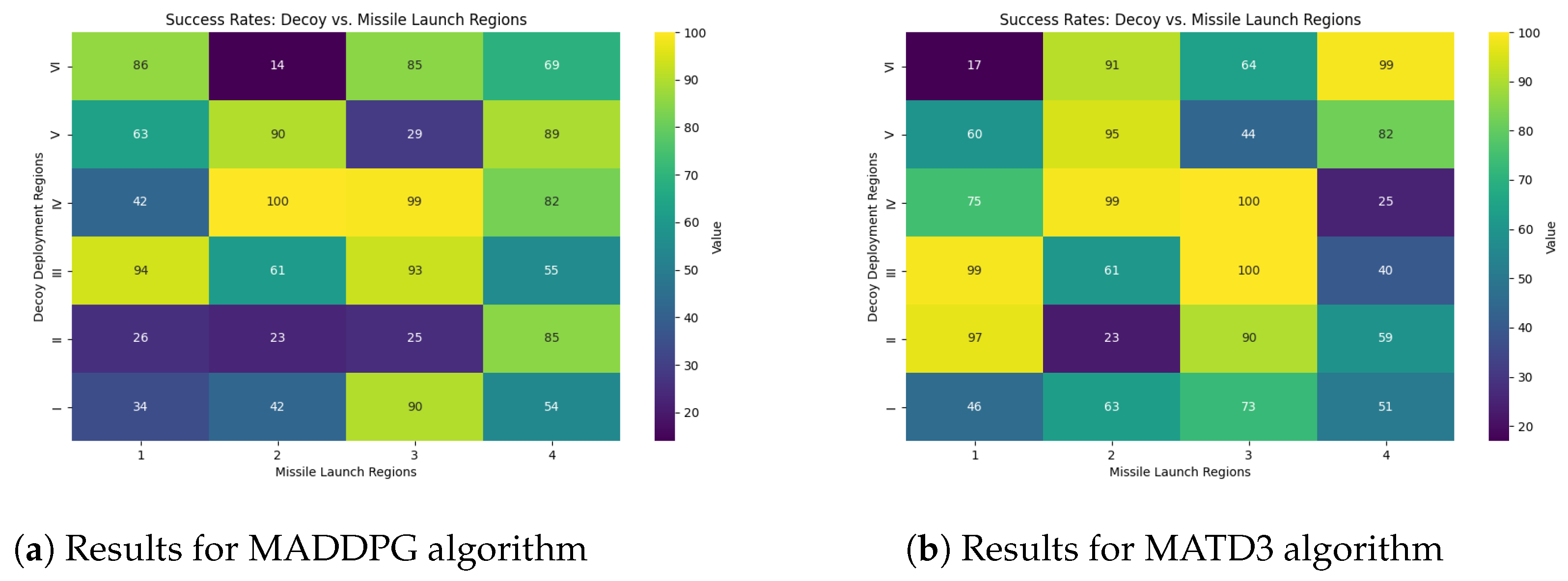
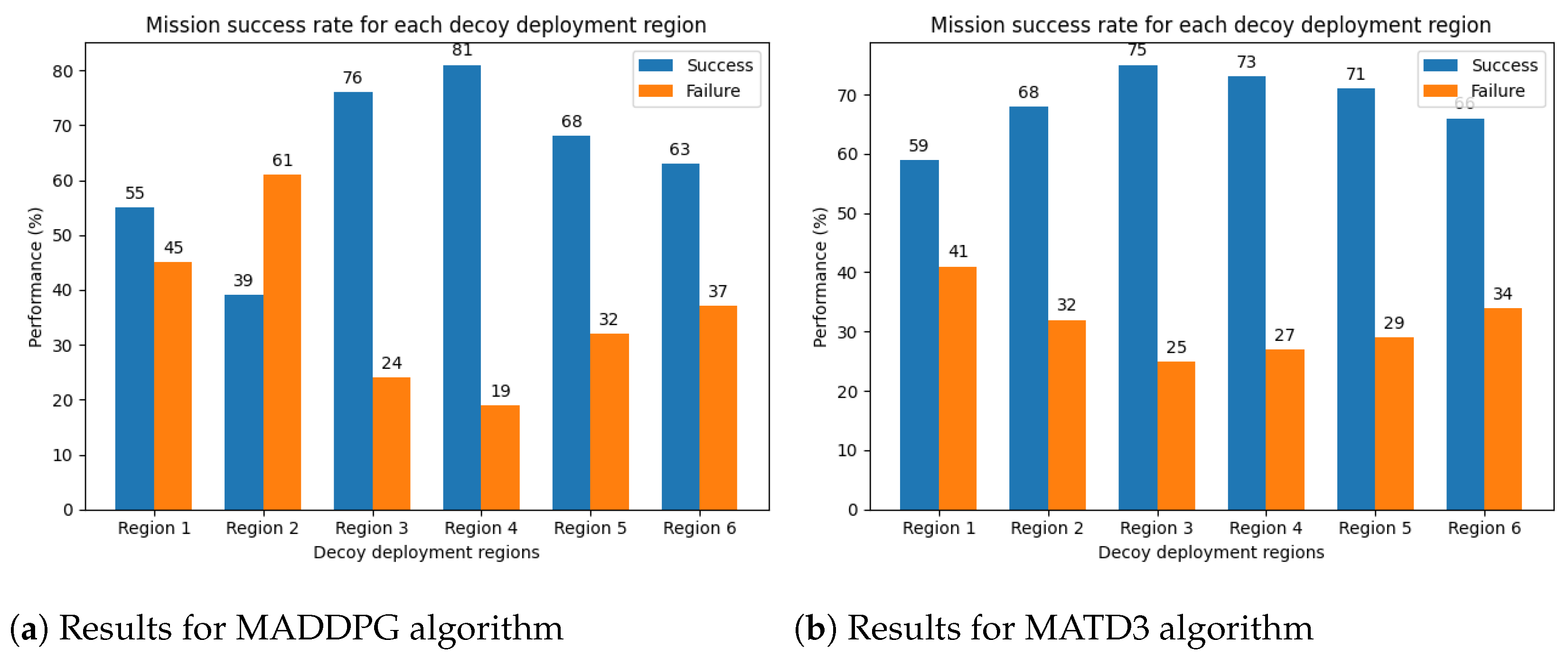
5.1. Evaluation Based on the Variable Decoy Deployment Region and Missile Launch Direction

In the first case, we set constant default values for the maximum speed of the decoy and the missile speed. This allowed us to analyze the impact of the decoy deployment regions and missile launch direction on the mission success rate. As seen in Figure 7, we generate six different regions for decoy deployment, and the missile can be launched from one of four different points. This setup results in a 6 by 4 matrix, allowing us to observe which combination provides the most protection for the main platform.

To evaluate the effectiveness of the proposed approach for each combination of decoy deployment region and missile launch direction, we employed a Monte Carlo simulation technique using trained decoys, conducting a total of 10,000 simulations. In each run, decoys were randomly deployed to a region, and the missile was launched from one of the pre-defined points. The decoy can reach a maximum speed of 20 m/s, the target ship moves at 15 m/s, and the missile speed is 300 m/s. After each termination, we record the outcomes for subsequent analysis, such as determining the success rate. The episode terminates when the missile strikes either the real target or a decoy.

Decoys were trained separately using the MADDPG and MATD3 algorithms, with the same hyperparameters and number of neurons per hidden layer. After the Monte Carlo simulations, the success rates were visualized using a heat map for each deployment region and launch direction combination. As indicated in Figure 8, the columns depict missile launch directions, while the rows represent decoy deployment regions, and both of which are defined in Figure 7.

Each cell value in the heat map represents the percentage effectiveness of the proposed decoy deployment strategy against the missile threat. We can derive key insights regarding the effectiveness of the strategy by examining the success rates of the decoy deployment regions against the missile threat direction.

Let us begin our analysis of Figure 8a by focusing on the decoy deployment regions. There is a noticeable variation in decoys’ efficiency based on the regions from which the missile is launched. When decoys are dispatched to the fourth deployment region, they successfully execute the mission with percentages of 42, 100, 99, and 82. This implies that the fourth decoy deployment strategy is reliable and adaptable to a variety of missile launch scenarios. In contrast, the sixth decoy deployment region is prominently inconsistent, with success rates varying between 86 against the first missile launch direction and 14 against the second missile launch direction.

The data in Figure 8b show the mission success rate for decoys rained by the MATD3 algorithm. The investigation’s findings indicate that regions 3 and 4 are the most effective for deploying decoys against the missile threat among the six decoy deployment regions. Regions 2 and 5 are moderately effective against the approaching missile threat and can be considered secondary options, especially in non-critical scenarios or to complement more effective regions.

Figure 9a,b present bar charts depicting the performance of the proposed decoy deployment strategy across different deployment regions, regardless of the missile launch direction. The decoys trained using the MADDPG algorithm achieve a success rate of 81% against incoming missile threats, while those trained with the MATD3 algorithm achieve a 75% success rate against threats from any direction.

5.2. Evaluation with Variable Decoys’ Maximum Speed and Missile Speed

In the second case, we examine how the maximum speed of decoys and the speed of missile influence the performance of the proposed strategy. The decoy speeds considered are 20, 25, 30, 35, and 40 in m/s, while the missile speeds are analyzed at Mach numbers 0.7, 0.8, 0.9, 1.0, and1.1.

Table 3. Decoy Performance for MADPPG algorithm [25].

	Missile Speed (in Mach)
Decoy Speed	0.7	0.8	0.9	1	1.1
20	64.8	67.1	66.26	66.27	66.02
25	65.6	65.8	65.7	65.75	66.07
30	65.8	65.65	65.6	65.39	65.16
35	64.9	64.8	64.62	64.41	64.34
40	64.13	63.86	63.81	63.73	63.56

shows the success rates of the decoy deployment strategy trained by the MADDPG algorithm. There appears to be no linear relationship between the success rate and the speeds of both the decoys and the missile. In general, as the missile’s speed increases, the time available for decoys to successfully carry out their mission decreases. As the speed of the decoys increases, the likelihood of them moving out of the radar seeker’s field of view rises, negatively impacting the mission’s success. The highest performance is observed with a success rate of 67.1%, achieved when the maximum decoy speed is 20 m/s and the missile speed is 0.8 Mach.

Similar to Table 3,

Table 4. Decoy Performance for MATD3 algorithm [27].

	Missile Speed (in Mach)
Decoy Speed	0.7	0.8	0.9	1	1.1
20	69.2	69.7	69.1	68.2	68.62
25	68.76	69.07	69.2	69.01	68.99
30	68.9	69.07	68.93	69.05	69.06
35	68.97	68.82	68.62	68.55	68.38
40	68.22	68.01	67.83	67.62	67.42

records the highest success rate of 69.7% for a decoy speed of 20 m/s and a missile speed of 0.8 Mach. This suggests that with a maximum decoy speed of 20 m/s, the deployment strategy can effectively counter missile threats across various Mach values.

5.3. Robustness Evaluation of Trained Decoys under Noisy Conditions

To evaluate the robustness of trained decoys under more realistic, noisy conditions—such as those that may arise from imperfections in sensor data—we introduce noise to all observation parameters. We consider five levels of noise, expressed as percentages, which are multiplied by the normalized observation parameters (ranging from 0 to 1). The noise levels applied are 5%, 10%, 15%, 20%, and 25% of the nominal parameters. The resulting observation data is the sum of the nominal values and the noise-adjusted values. In this comparison, the missile is consistently launched from the same area, and decoys are deployed in the same direction. Specifically, the missile is launched from direction 1, with the decoy deployment angle set to 60 degrees. As shown in Figure 10, we compare the obtained results with the baseline (noise-free) performance. The trained decoys perform well at noise levels of 5%, 10%, and 15%, achieving mission success rates of 36%, 36%, and 35%, respectively. However, at noise levels of 20% and 25%, the performance rate declines to 32% and 29%, respectively. Our analysis indicates the decoys perform efficiently at low noise levels but deteriorate as noise increases, suggesting training improvements.

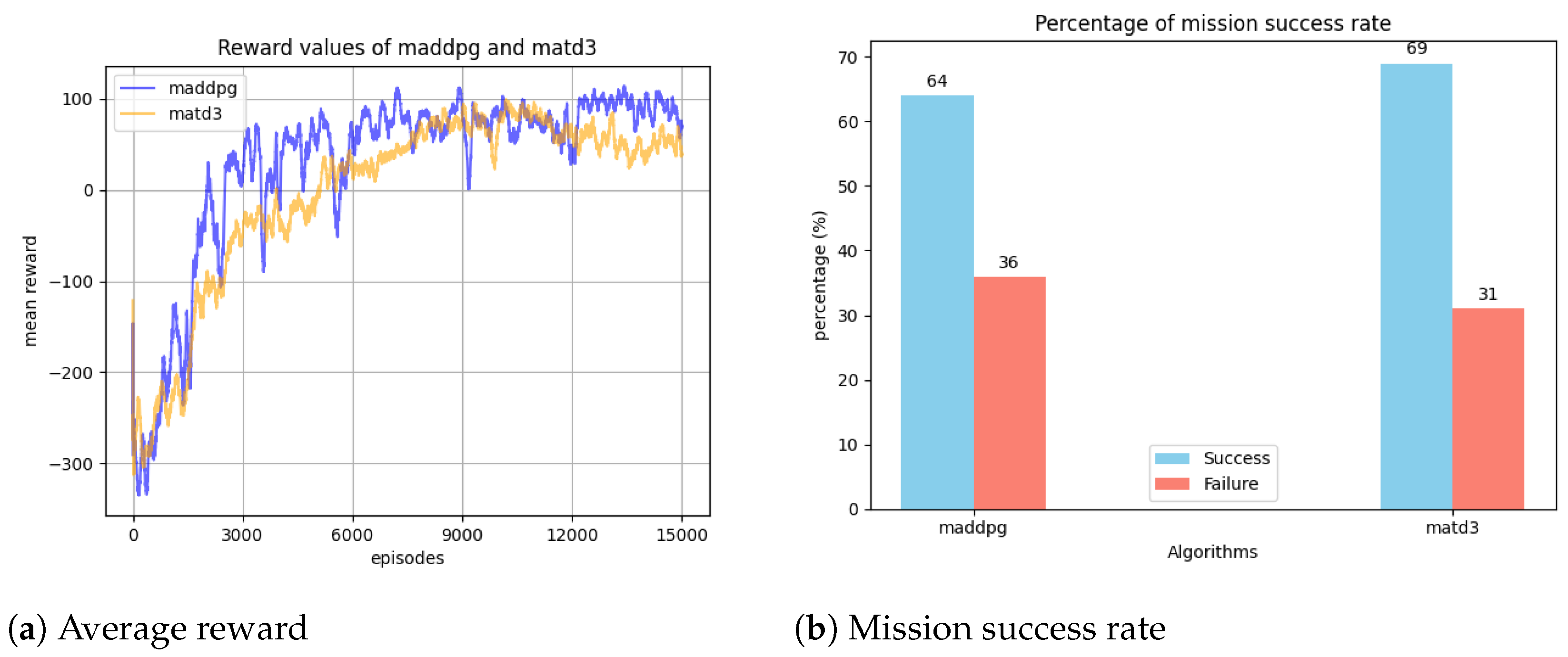
5.4. Comparisons of MADDPG and MATD3 Algorithms

In the envisioned scenario, the mission of the decoys is to protect the target ship from the approaching missile threat. To achieve this effectively, the decoys are trained separately using the MADDPG and MATD3 algorithms. Figure 11a illustrates the average reward values for both algorithms during training. The figure shows no significant difference between the two reward curves, although MADDPG occasionally achieves higher reward values than MATD3. Figure 11b compares the overall mission success rates for these algorithms, revealing that MATD3 achieves a higher performance with a 69% success rate, while MADDPG attains 64%. The effectiveness of decoys in deceiving missile threats largely depends on their formation. Based on the success rate values, it can be inferred that decoys trained using the MATD3 algorithm execute swarm formations more effectively than those trained with the MADDPG algorithm.

6. Conclusions

In this study, we develop a reinforcement-learning-based decoy deployment strategy aimed at enhancing the survival probability of a target ship. In total, three decoys are deployed from the ship’s deck to operate cooperatively to accomplish their mission. We utilize the MADDPG (Multi-Agent Deep Deterministic Policy Gradient) and MATD3 (Multi-Agent Twin Delayed Deep Deterministic Policy Gradient) algorithms to train the decoys in cooperative behavior. The deployment strategy designates one decoy as the leader and the others as followers, utilizing a circular formation to maintain proximity and effective coordination among them. We evaluate the performance of the proposed approach using four critical parameters: the decoy deployment regions, the missile launch direction, the maximum speed of the decoys, and the missile speed. Results show that among the six decoy deployment regions, regions 3, 4, and 5 are the most effective for deploying decoys to counter missile threats, regardless of the direction of the missiles approach. Comparing different maximum decoy speeds, the findings demonstrate that a deployment strategy with a maximum decoy speed of 20 m/s is effective in countering missile threats across various Mach values. The decoys trained using the MATD3 algorithm achieved a 69% mission success rate, outperforming those trained with the MADDPG algorithm, which attained a 64% success rate.

We acknowledge that our approach has certain limitations, particularly the longer duration required to establish swarm formation configuration after deployment. However, thanks to the independent decision-making capability our approach provides to the decoys, they are able to maneuver effectively in dynamic warfare environments.

This study initially considers the RCS level based on a single scatterer. However, multiple scatter points are considered to calculate a combined RCS level for the target to achieve a more comprehensive analysis. This approach allows for a more realistic evaluation of the performance of the proposed decoy deployment strategy.

References

1. Kerins, W.J. Analysis of towed decoys. IEEE Trans. Aerosp. Electron. Syst. 1993, 29, 1222–1227. [Google Scholar] [CrossRef]
2. Yeh, J.H. Effects of Towed-Decoys against an Anti-Air Missile with a Monopulse Seeker. Ph.D. Thesis, Naval Postgraduate School, Monterey, CA, USA, 1995. [Google Scholar]
3. Zhou, Y. Correlation parameters simulation for towed radar active decoy. In Proceedings of the 2012 International Conference on Computer Distributed Control and Intelligent Environmental Monitoring, Zhangjiajie, China, 5–6 March 2012; pp. 214–217. [Google Scholar]
4. Tan, T.H. Effectiveness of Off-Board Active Decoys against Anti-Shipping Missiles; Technical Report; Naval Postgraduate School: Monterey, CA, USA, 1996. [Google Scholar]
5. Lakshmi, E.V.; Sastry, N.; Rao, B.P. Optimum active decoy deployment for effective deception of missile radars. In Proceedings of the 2011 IEEE CIE International Conference on Radar, Chengdu, China, 24–27 October 2011; Volume 1, pp. 234–237. [Google Scholar]
6. Butt, F.A.; Jalil, M. An overview of electronic warfare in radar systems. In Proceedings of the 2013 the International Conference on Technological Advances in Electrical, Electronics and Computer Engineering (TAEECE), Konya, Turkey, 9–11 May 2013; pp. 213–217. [Google Scholar]
7. Ragesh, R.; Ratnoo, A.; Ghose, D. Analysis of evader survivability enhancement by decoy deployment. In Proceedings of the 2014 American Control Conference, Portland, OR, USA, 4–6 June 2014; pp. 4735–4740. [Google Scholar]
8. Rim, J.W.; Jung, K.H.; Koh, I.S.; Baek, C.; Lee, S.; Choi, S.H. Simulation of dynamic EADs jamming performance against tracking radar in presence of airborne platform. Int. J. Aeronaut. Space Sci. 2015, 16, 475–483. [Google Scholar] [CrossRef]
9. Ragesh, R.; Ratnoo, A.; Ghose, D. Decoy Launch Envelopes for Survivability in an Interceptor–Target Engagement. J. Guid. Control Dyn. 2016, 39, 667–676. [Google Scholar] [CrossRef]
10. Rim, J.W.; Koh, I.S.; Choi, S.H. Jamming performance analysis for repeater-type active decoy against ground tracking radar considering dynamics of platform and decoy. In Proceedings of the 2017 18th International Radar Symposium (IRS), Prague, Czech Republic, 28–30 June 2017; pp. 1–9. [Google Scholar]
11. Rajagopalan, A. Active Protection System Soft-Kill Using Q-Learning. In Proceedings of the International Conference on Science and Innovation for Land Power, Australia Defence Science and Technology, online, 5–6 September 2018. [Google Scholar]
12. Rim, J.W.; Koh, I.S. Effect of beam pattern and amplifier gain of repeater-type active decoy on jamming to active RF seeker system based on proportional navigation law. In Proceedings of the 2018 19th International Radar Symposium (IRS), Bonn, Germany, 20–22 June 2018; pp. 1–9. [Google Scholar]
13. Kim, K. Engagement-Scenario-Based Decoy-Effect Simulation Against an Anti-ship Missile Considering Radar Cross Section and Evasive Maneuvers of Naval Ships. J. Ocean Eng. Technol. 2021, 35, 238–246. [Google Scholar] [CrossRef]
14. Chen, Y.; Wang, H.; Zhao, Y. Optimal trajectory for swim-out acoustic decoy to countermeasure torpedo. In Proceedings of the Fourth International Workshop on Advanced Computational Intelligence, Wuhan, China, 19–21 October 2011; pp. 86–91. [Google Scholar]
15. Kwon, S.J.; Seo, K.M.; Kim, B.S.; Kim, T.G. Effectiveness analysis of anti-torpedo warfare simulation for evaluating mix strategies of decoys and jammers. In Proceedings of the Advanced Methods, Techniques, and Applications in Modeling and Simulation: Asia Simulation Conference 2011, Seoul, Republic of Korea, 16–18 November 2011; pp. 385–393. [Google Scholar]
16. Chen, Y.C.; Guo, Y.H. Optimal combination strategy for two swim-out acoustic decoys to countermeasure acoustic homing torpedo. In Proceedings of the 2017 4th International Conference on Information Science and Control Engineering (ICISCE), Changsha, China, 21–23 July 2017; pp. 1061–1065. [Google Scholar]
17. Akhil, K.; Ghose, D.; Rao, S.K. Optimizing deployment of multiple decoys to enhance ship survivability. In Proceedings of the 2008 American Control Conference, Seattle, WA, USA, 11–13 June 2008; pp. 1812–1817. [Google Scholar]
18. Conte, C.; Verini Supplizi, S.; de Alteriis, G.; Mele, A.; Rufino, G.; Accardo, D. Using Drone Swarms as a Countermeasure of Radar Detection. J. Aerosp. Inf. Syst. 2023, 20, 70–80. [Google Scholar] [CrossRef]
19. Shames, I.; Dostovalova, A.; Kim, J.; Hmam, H. Task allocation and motion control for threat-seduction decoys. In Proceedings of the 2017 IEEE 56th Annual Conference on Decision and Control (CDC), Melbourne, Australia, 12–15 December 2017; pp. 4509–4514. [Google Scholar]
20. Jeong, J.; Yu, B.; Kim, T.; Kim, S.; Suk, J.; Oh, H. Maritime application of ducted-fan flight array system: Decoy for anti-ship missile. In Proceedings of the 2017 Workshop on Research, Education and Development of Unmanned Aerial Systems (RED-UAS), Linkoping, Sweden, 3–5 October 2017; pp. 72–77. [Google Scholar]
21. Dileep, M.; Yu, B.; Kim, S.; Oh, H. Task Assignment for Deploying Unmanned Aircraft as Decoys. Int. J. Control Autom. Syst. 2020, 18, 3204–3217. [Google Scholar] [CrossRef]
22. Li, J.; Zhang, G.; Zhang, X.; Zhang, W. Integrating dynamic event-triggered and sensor-tolerant control: Application to USV-UAVs cooperative formation system for maritime parallel search. IEEE Trans. Intell. Transp. Syst. 2023, 25, 3986–3998. [Google Scholar] [CrossRef]
23. Yu, C.; Velu, A.; Vinitsky, E.; Wang, Y.; Bayen, A.; Wu, Y. The Surprising Effectiveness of PPO in Cooperative, Multi-Agent Games. arXiv 2021, arXiv:2103.01955. [Google Scholar]
24. Foerster, J.; Farquhar, G.; Afouras, T.; Nardelli, N.; Whiteson, S. Counterfactual Multi-Agent Policy Gradients. arXiv 2018, arXiv:1705.08926. [Google Scholar] [CrossRef]
25. Lowe, R.; Wu, Y.I.; Tamar, A.; Harb, J.; Pieter Abbeel, O.; Mordatch, I. Multi-agent actor-critic for mixed cooperative-competitive environments. arXiv 2017, arXiv:1706.02275. [Google Scholar]
26. Lillicrap, T.P.; Hunt, J.J.; Pritzel, A.; Heess, N.; Erez, T.; Tassa, Y.; Silver, D.; Wierstra, D. Continuous control with deep reinforcement learning. arXiv 2015, arXiv:1509.02971. [Google Scholar]
27. Ackermann, J.; Gabler, V.; Osa, T.; Sugiyama, M. Reducing overestimation bias in multi-agent domains using double centralized critics. arXiv 2019, arXiv:1910.01465. [Google Scholar]
28. Fujimoto, S.; Hoof, H.; Meger, D. Addressing function approximation error in actor-critic methods. In Proceedings of the International Conference on Machine Learning, PMLR, Stockholm, Sweden, 10–15 July 2018; pp. 1587–1596. [Google Scholar]
Figure 1. High-Level Diagram of the Proposed Methodology.
Aerospace 11 00684 g001
Figure 2. Trajectories of the missile, target, and decoys.
Aerospace 11 00684 g002
Figure 3. Missile Target engagement.
Aerospace 11 00684 g003
Figure 4. Reinforcement Learning Environment.
Aerospace 11 00684 g004
Figure 5. Centralized training and decentralized execution multi-agent reinforcement learning framework.
Aerospace 11 00684 g005
Figure 6. Relative position of leader agent with goal point and follower agents.
Aerospace 11 00684 g006
Figure 7. Decoy deployment regions and angles.
Aerospace 11 00684 g007
Figure 8. Mission success rate based on the decoy deployment regions and missile launch direction.
Aerospace 11 00684 g008
Figure 9. Mission success rate irrespective of missile launch direction.
Aerospace 11 00684 g009
Figure 10. The impact of noise in the mission success rate.
Aerospace 11 00684 g010
Figure 11. Average reward curve (left) and mission success rate (right) for MADDPG and MATD3 algorithms.
Aerospace 11 00684 g011