The Dynamic Prediction Method for Aircraft Cabin Temperatures Based on Flight Test Data

Abstract

For advanced aircraft, the temperature environment inside the cabin is very severe due to the high flight speed and the compact concentration of the electronic equipment in the cabin. Accurately predicting the temperature environment induced inside the cabin during the flight of the aircraft can determine the temperature environment requirements of the onboard equipment inside the cabin and provide an accurate input for the thermal design optimization and test verification of the equipment. The temperature environment of the whole aircraft is divided into zones by the cluster analysis method; the heat transfer mechanism of the aircraft cabin is analyzed for the target area; and the influence of internal and external factors on the thermal environment is considered to establish the temperature environment prediction model of the target cabin. The coefficients of the equations in the model are parameterized to extract the long-term stable terms and trend change terms; with the help of the measured data of the flight state, the model coefficients are determined by a stepwise regression method; and the temperature value inside the aircraft cabin is the output by inputting parameters such as flight altitude, flight speed, and external temperature. The model validation results show that the established temperature environment prediction model can accurately predict the change curve of the cabin temperature during the flight of the aircraft, and the model has a good follow-up performance, which reduces the prediction error caused by the temperature hysteresis effect. For an aircraft, the estimated error is 2.8 °C at a confidence level of 95%. Engineering cases show that the application of this method can increase the thermal design requirements of the airborne equipment by 15 °C, increase the low-temperature test conditions by 17 °C, and avoid the problems caused by an insufficient design and over-testing. This method can accurately predict the internal temperature distribution of the cabin during the flight state of the aircraft, help designers determine the thermal design requirements of the airborne equipment, modify the thermal design and temperature test profile, and improve the environmental worth of the equipment.

1. Introduction

The induced environment inside the aircraft cabin is the local environment generated by the combined effects of the aircraft platform, other equipment inside the cabin, and the equipment itself [1]. In recent years, with the improvements in aircraft combat technical indicators, on the one hand, its flight speed has increased significantly, and aerodynamic heating has become more serious. At the same time, due to volume requirements, the equipment inside the aircraft cabin has become more concentrated and compact, which has affected the heat dissipation effect, resulting in a very severe high temperature environment inside the cabin. On the other hand, when the aircraft is flying at a high altitude and a low speed with a long flight time, the external natural environment is extremely low, which will also lead to an extremely low temperature environment inside the cabin. Whether it is a high or low temperature will have a serious impact on the internal products of the aircraft, such as structural deformation, material aging, seal failure, increased lubricant viscosity, and electrical performance degradation, thereby causing a series of failures. The statistics show that 52% of aircraft’s onboard equipment failures are caused by the environment, while 74% are caused by environmental factors such as platform-induced vibration and temperature, with temperature having the most serious impact [2]. In order to reduce the risk of onboard equipment failures caused by the temperature environment, it is necessary to determine the temperature environment data of the equipment throughout its life cycle as much as possible. Flight testing is a common method for obtaining the cabin temperature environment data. However, due to the high cost and difficulty of flight testing, it is often difficult to obtain the most severe extreme temperature environment data due to the time window and safety restrictions. Therefore, temperature environment prediction technology has become a focus of attention for various countries. Moreover, determining the temperature environment requirements early in the design stage is also a development trend in the future of aircraft development [3,4], which also requires accurate temperature prediction technology.

The prediction methods for the induced temperature environment are mainly divided into two categories: numerical simulations and data-driven predictions [5]. Between the two, the data-driven method has been widely used in engineering due to its advantage of a fast calculation speed. The data-driven method mainly relies on flight test data to achieve temperature environment predictions through statistical induction, neural network, or heat transfer analysis methods. Based on temperature test data, ref. [6] established a linear model of the cabin temperature and the outside temperature when the aircraft was parked; ref. [7] analyzed the flight test data of the aircraft nacelle and calculated the temperature variation trend with altitude; ref. [8] counted the data on the temperature of the electronic pod under different conditions; ref. [9] calculated the high-temperature test conditions based on the measured missile storage data; ref. [10] established a linear regression model for predicting the rocket propellant temperature; ref. [11] established a polynomial model of the internal temperature of the container and the external temperature; ref. [12] used a BP neural network to predict the fuse temperature; refs. [13,14] used the Elman neural network to predict the cabin temperature of a UAV in the flight state and the seeker temperature of a missile in the storage state; ref. [15] used the ARX model to predict the temperature of the aircraft power system; ref. [16] used the ARIMA model to predict the temperature of the electrical equipment; ref. [17] used the RVFL neural network to predict the temperature environment of the wing pod; ref. [18] used a BP neural network to predict the temperature of the aircraft wing assembly frame; ref. [19] used the RVFL neural network to predict the temperature of the equipment compartment; ref. [20] applied a process neural network to predict the transient temperature of spacecraft; and ref. [21] used the advanced time series processing module net model to predict the satellite temperature. However, the above statistical induction and neural network methods rely entirely on the distribution patterns of the data themselves for prediction, lack basic theoretical support, and are limited by data samples; furthermore, the extrapolation effect of the model needs to be improved. Ref. [22] predicted the temperature of the aircraft rear fuselage skin by establishing a multimodal thermal model; ref. [23] established a heat transfer model for the cabin temperature of an aircraft and solved the temperature by solving the differential equation; ref. [24] applied the thermal network method to establish the thermal balance equation of the missile storage state and realized the prediction of the seeker temperature; ref. [25] established the thermal balance equation of the electronic equipment compartment of a high-altitude long-flight UAV and predicted the temperature change in the equipment compartment; ref. [26] analyzed the formation mechanism of the temperature environment of a helicopter in a parking state and established a temperature environment prediction model for the cockpit in a parking state; refs. [27,28] obtained the temperature changes of aircraft fuel tanks and aviation high-speed gears through thermal analysis; ref. [29] conducted a heat transfer analysis of airborne equipment and established a temperature prediction model for the finned tube storage energy system; and ref. [30] established a thermal analysis and prediction model for the motor slot of an electric aircraft. The heat transfer analysis method takes into account both the physical theory and flight data, but, due to the excessive idealization and simplification of the model parameters in the modeling process and insufficient consideration of thermal inertia, the temperature prediction has a lag phenomenon, and the prediction accuracy needs to be improved.

The model extrapolation effect and prediction accuracy are the problems that plague current temperature environment prediction work. In order to solve the above problems, the prediction accuracy of the temperature environment inside the aircraft cabin can be further improved, the temperature environment of the equipment during its life cycle in the cabin can be obtained, and an accurate input can be provided for the equipment’s thermal design and test verification. Based on the heat transfer theory, this paper proposes a temperature environment prediction algorithm with parameter optimization. Compared with traditional research, this algorithm establishes the heat transfer equation by deeply analyzing the heat transfer mechanism in physics, providing scientific theoretical support for ensuring the extrapolation effect of the model. At the same time, when solving the equation, different from the traditional method of roughly simplifying the variables to constants, this article carefully considers the changes in various physical quantities, and further combines them into unchanging constant terms and function terms that change with the flight state according to their change characteristics, thereby achieving a more accurate solution to the equation. After the above optimization, the algorithm establishes a functional relationship between the flight profile and the temperature environment, solves the model, and verifies the extrapolation effect based on the flight test data, eliminating the time lag of the predicted temperature change to improve the accuracy of the prediction of the dynamic change in the temperature environment. Engineering application cases show that research solving the problems of the inability to measure the limit profile in the flight test and the inaccurate requirements of the thermal design and test verification can determine the thermal design requirements in the early stages of design, reduce the cost of modifying the thermal design plans in the later stages of the design due to an inaccurate input, avoid insufficient assessment due to under-testing and increased costs due to over-testing, and are of great significance to aircraft development.

2. Methods

2.1. Temperature Environment Partitions

For a particular aircraft, a series of thermocouple sensors are used to measure the temperature data of the entire aircraft in flight, with the measurements covering 31 compartments of the entire aircraft, including the equipment compartment, the cockpit, and so on. The measurement points set U = {U1, U2, …, U31}. Since the measurement points are numerous and scattered, in order to facilitate modeling, the Kalman filter method is first applied to filter out the noise and interference signals while retaining the data features [31]. The temperature environment of the entire aircraft is partitioned to merge the data from similar measurement points.

The temperature environment partition of the whole aircraft is mainly divided into two steps: the first is structural partition. According to the structural characteristics of the aircraft and its surrounding thermal environment, a relatively broad preliminary partition result is given. According to the structure, it is mainly divided into three areas: the Forepart, Central and Rear; the second is data partition. Combined with the measured data, by calculating the average distance of the class, each measurement point is clustered and analyzed to further refine the partition results. The specific calculation method is as follows [32]:

$$d_{ij}(q)={[{{\displaystyle \sum _{k=1}^p\left|x_{ik}-x_{jk}\right|}}^q]}^{1/q}$$

(1)

$${D_{KL}}^2={\displaystyle \frac{1}{n_K{n}_L}}{\displaystyle \sum _{x_i\in U_K,x_j\in U_L}{d_{ij}}^2}$$

(2)

$${D_{MJ}}^2={\displaystyle \frac{n_K}{n_M}}{D_{KJ}}^2+{\displaystyle \frac{n_L}{n_M}}{D_{LJ}}^2$$

(3)

After calculation, the partition results of the whole materiel are determined as shown in

Table 1. The result of the temperature environment partition.

Structural Partitions	Data Set	Cluster Partitioning	Data Set
Forepart	U1, U2, …, U6	Zone 1	U1
		Zone 2	U2, U3
		Zone 3	U4, U5, U6
Central	U7, U8, …, U24	Zone 4	U7, U8
		Zone 5	U9, U10, …, U18
		Zone 6	U19, U20, …, U24
Rear	U25, U26, …, U30	Zone 7	U25, U26, U28
		Zone 8	U29, U31
		Zone 9	U27, U30

, where the results are obtained by combining the structural layout partitioning with cluster analysis calculations. The Forepart is mainly located near the head of the aircraft, including the radar cabin, cockpit, etc. Its characteristics are that it faces the opposite airflow head-on, the airflow speed changes rapidly, and the cabin airtightness is good; it is mainly affected by aerodynamic heating and equipment heating. The Central is the middle area of the fuselage, including the landing gear bay, weapon bay, etc. The structural changes are relatively gentle, the airflow speed is stable, and the air tightness is not as good as the front part. It is mainly affected by aerodynamic heating, the heating of the electronic equipment, and the ram air. The Rear is the rear end area of the aircraft, including the engine compartment and surrounding compartments. Its structural changes are relatively gentle, but the thermal environment is greatly affected by engine combustion. Based on the above division into the Forepart, Central, and Rear areas, the Minkowski distance is determined by a cluster analysis. With respect to these areas, the distance between U₂ and U₃ is shorter and the distance between U₄, U₅, and U₆ is shorter, which means that their data distribution patterns are similar and can be considered as the same area; therefore, the Forepart is further divided into Zone 1, Zone 2, and Zone 3. Similarly, based on the data’s similarity, the Central is further divided into Zone 4, Zone 5, and Zone 6; and the Rear is further divided into Zone 7, Zone 8, and Zone 9. The number of measuring points in each area is different, but the values and changing trends of the data are relatively consistent.

2.2. Thermal Environment Analysis

Analyzing the formation mechanism of the whole materiel’s thermal environment during the flight of the aircraft, the formation of the whole materiel’s thermal environment can be decomposed into the following nine thermal physical processes:

• The aerodynamic thermal effect between the high-speed flow outside the aircraft and the skin;
• The radiation effect of the sun on the outer surface of the aircraft skin and the radiation heat exchange effect between the outer surface of the skin and the space environment, which comprehensively form the non-uniform radiation heat exchange field on the outer surface of the equipment skin;
• The exchange of airflow inside the aircraft’s non-airtight cabin and the airflow of the external atmospheric environment, including the cooling of the cabin by the ram air;
• The internal heat conduction process of the skin under the coupling of the internal and external thermal environments of the aircraft;
• The heat conduction–convection–radiation-coupled heat exchange process formed between the inner surface of the skin and the internal airflow and structural equipment of the equipment, which is a multimodal-coupled heat exchange process in a large and complex system;
• The heat exchange between the environmental control system and the equipment. After the environmental control intake and the airflow inside the equipment are mixed and exchanged, convection heat exchange occurs with the equipment inside the aircraft;
• The airflow and structural heat conduction between adjacent cabins;
• The heat generated by the equipment operation;
• The heat release from the engine combustion.

For different areas of the entire materiel, the formation of the thermal environment is nothing more than the above form, but, due to the different areas, the influence of various physical processes is different, and the engineering simplification is also different.

2.3. Dynamic Prediction Model Establishment

Based on the partition results of the whole aircraft in Table 1, this paper selects Zone 1 as an example to analyze its thermal environment in detail. A schematic diagram of the location of Zone 1 is shown in Figure 1.

However, before building the model, there are some assumptions that need to be explained, as follows:

• It is assumed that air is an ideal gas and its physical properties satisfy the ideal gas state equation.
• It is assumed that the air temperature is evenly distributed in the same area.
• Assuming that the aircraft skin is very thin, it is assumed that the area inside and outside the skin is approximately equal.
• It is assumed that the gas pressure in the cabin remains constant and the airflow in and out of the cabin is equal.

Zone 1 is mainly the radar antenna cabin of the aircraft, adjacent to Zone 2, and located at the head of the fuselage. Since it is far away from the engine, the influence of the engine combustion heat release can be ignored. Since the projected area of the aircraft exposed to solar radiation is small during flight and the reflectivity of the outer skin is high, the influence of solar radiation on the thermal environment of the cabin air can be ignored. Therefore, the air inside the cabin of Zone 1 is mainly affected by the convection heat transfer on the inner surface of the skin, the ram air heat transfer, the heat transfer of the adjacent cabins, and the heating of the electronic equipment in the cabin. Its heat flow equation is shown as follows:

$$c_1{m}_1{\displaystyle \frac{\partial T_1\left(t\right)}{\partial t}}=Q_{T_r}\left(t\right)+Q_m\left(t\right)+Q_c\left(t\right)+Q_E\left(t\right)$$

(4)

Aerodynamic heating is mainly achieved by heating the outer surface of the skin through high-speed airflow, and then the heat is conducted from the outer surface of the skin to the inner surface of the skin, before finally the inner surface and the air in the cabin exchange heat together. Since the curvature of the fuselage skin is large, it is assumed that the skin is a thin flat plate structure, and the aerodynamic heating amount Q_Tr is calculated as follows:

$$Q_{T_r}(t)={\displaystyle \frac{A}{\frac{1}{h_1}+\frac{1}{h_2}+\frac{\delta }{\lambda }}}(T_r(t)-T_1(t))$$

(5)

The calculation method of T_r is as follows [33]:

$$T_r=(T_H+273.15)\times (1+\gamma {\displaystyle \frac{k-1}{2}}M{a}^2)-273.15$$

(6)

The heat exchange between the cabin air and outside air is mainly caused by the ram air entering the cabin. Assuming that the ram air velocity is approximately equal to the flight speed, the heat exchange Q_m is calculated as follows:

$$Q_m(t)=m_{r-1}{c}_r{T}_r(t)-m_{r-1}{c}_1{T}_1(t)$$

(7)

The heat transfer between the cabins is mainly caused by the structural heat conduction and airflow. The specific calculation is shown as follows:

$$Q_c\left(t\right)={\displaystyle \sum _{i=1}^{n_1}(R_i(T_i(t)-T_1(t))+c_1{m}_i(T_i(t)-T_1(t))}$$

(8)

The heat dissipation of the electronic equipment is unknown, so we take the constant Q_E0 as the basic heat dissipation of the electronic equipment. Assuming that the thermal power of the electronic equipment changes with time, the thermal power of the electronic equipment during flight is as follows:

$$Q_E\left(t\right)=Q_{E0}\times t^{n_0}$$

(9)

Combining Equations (5)–(9), Equation (4) is further transformed into Equation (10), as follows:

$$c_1{m}_1{\displaystyle \frac{\partial T_1\left(t\right)}{\partial t}}={\displaystyle \frac{A}{\frac{1}{h_1}+\frac{1}{h_2}+\frac{\delta }{\lambda }}}(T_r(t)-T_1(t))+c_r{m}_{r-1}{T}_r(t)-c_1{m}_{1-r}{T}_1(t)+R_2(T_2(t)-T_1(t))+c_1{m}_2(T_2(t)-T_1(t))+Q_{E0}\times t^{n_0}$$

(10)

According to the measured data, the internal temperature of the cabin is known, so if the various coefficients are assumed to be constants, relatively accurate model parameters can be obtained through data regression. However, in the actual process, only the geometric structure parameters, such as the skin thickness $\delta$ and the area A are constants, and other variables can be regarded as functions of temperature. Therefore, in order to obtain accurate model parameters, Equation (10) is further decomposed and transformed.

The specific heat capacity c₁ of the cabin air is calculated as follows [34]:

$$c_1=\left\{\begin{array}{c}1005-0.16\times T_1,(T_1\le 0°\mathrm{C})\\ 1005+0.04\times T_1,(0<T_1\le 120°\mathrm{C})\end{array}\right.$$

(11)

For the convection heat transfer coefficient $h_1$ of the outer skin surface, due to the drastic change in the external airflow, the calculation method is as follows [34,35]:

$$h_1={\displaystyle \frac{Nu{\lambda }_0}{l}}$$

(12)

$$Nu=\left\{\begin{array}{c}0.0332{\mathrm{Re}}^{1/2}{\mathrm{Pr}}^{1/3},LaminarFlow\\ 0.0296{\mathrm{Re}}^{4/5}{\mathrm{Pr}}^{2/5},TurbulentFlow\end{array}\right.$$

(13)

$${\lambda }_0={\displaystyle \frac{2.648\times {10}^{-3}\times (T_H+273.15{)}^{1.5}}{(T_H+273.15)+245.4\times {10}^{-\frac{12}{T_H+273.15}}}}$$

(14)

$$\mathrm{Re}={\displaystyle \frac{{\rho }_0{v}_{0}l}{\mu }}$$

(15)

$$\mathrm{Pr}={\displaystyle \frac{\mu c_0}{{\lambda }_0}}$$

(16)

The air density can be calculated using the ideal gas state equation as follows [36]:

$${\rho }_0=p/R\times (T_H+273.15)$$

(17)

The relationship between the atmospheric pressure p and the flight altitude is as follows [34]:

$$\begin{array}{l}p(H)=101325{(1-{\displaystyle \frac{H}{44330}})}^{{\displaystyle \frac{g}{0.0065R}}},(0\le H<11000\mathrm{m})\\ p(H)=22631.8\exp (-{\displaystyle \frac{H-11000}{6340}}),(11000\le H<20000\mathrm{m})\end{array}$$

(18)

The air velocity $v_0$ can be obtained from the relationship between the air velocity near the outer surface of the aircraft and the flight Mach number: the Mach number is the ratio of the air velocity to the local sound speed. It can be obtained from the flight parameter record information of the aircraft. The calculation of $v_0$ is as follows [36]:

$$v_0=Ma\sqrt{k{R}_0\times (T_H+273.15)}$$

(19)

The air viscosity coefficient $\mu$ is a function of the temperature, and the relationship is as follows [34]:

$$\mu ={\displaystyle \frac{1.458\times {10}^{-6}\times (T_H+273.15{)}^{1.5}}{(T_H+273.15)+110.4}}$$

(20)

Substitute Equations (11)–(20) into Equation (10), and further simplify and discretize them. The discretization method is the explicit difference, and the equation is as follows:

$$\begin{array}{ll}{k}_2(T_1^{(n+1)}(t)-T_1^{(n)}(t))=& C_1{k}_1(T_r^{(n)}(t)-T_1^{(n)}(t))+C_2{k}_1{k}_2{c}_r{T}_1^{(n)}(t)+C_3{k}_1{c}_r{T}_r^{(n)}(t)-C_4{k}_2{T}_1^{(n)}(t)-C_5{T}_1^{(n)}(t)+\\ & C_6{k}_1{k}_2(T_2^{(n)}(t)-T_1^{(n)}(t))+C_7{k}_1(T_2^{(n)}(t)-T_1^{(n)}(t))+C_8{k}_2(T_2^{(n)}(t)-T_1^{(n)}(t))+C_9(T_2^{(n)}(t)-T_1^{(n)}(t))+\\ & C_{10}{k}_1{t}^{n_0}-C_{11}(T_1^{(n+1)}(t)-T_1^{(n)}(t))\end{array}$$

(21)

where n is the relative time and the definitions of each coefficient are as follows:

$$k_1={\displaystyle \frac{1}{c_1}}$$

(22)

$$k_2={\displaystyle \frac{1}{h_1{l}^{0.2}}}$$

(23)

$$r_1={\displaystyle \frac{1}{h_2}}+{\displaystyle \frac{\delta }{\lambda }}$$

(24)

$$C_1={\displaystyle \frac{1}{l^{0.2}{m}_1}}$$

(25)

$$C_2=l^{0.2}{\displaystyle \frac{m_{r-1}}{m_1}}$$

(26)

$$C_3=r_1{\displaystyle \frac{m_{r-1}}{m_1}}$$

(27)

$$C_4=l^{0.2}{\displaystyle \frac{m_{1-r}}{m_1}}$$

(28)

$$C_5=r_1{\displaystyle \frac{m_{1-r}}{m_1}}$$

(29)

$$C_6=l^{0.2}{\displaystyle \frac{R_{12}}{m_1}}$$

(30)

$$C_7=r_1{\displaystyle \frac{R_{12}}{m_1}}$$

(31)

$$C_8=l^{0.2}{\displaystyle \frac{m_{12}}{m_1}}$$

(32)

$$C_9=r_1{\displaystyle \frac{m_{12}}{m_1}}$$

(33)

$$C_{10}={\displaystyle \frac{1}{m_1}}{Q}_{E0}$$

(34)

$$C_{11}=r_1$$

(35)

Analyzing Equations (22)–(35), assuming that the air quality inside the cabin remains unchanged, r₁ and C₁~C₁₁ can be regarded as constants and k₁ and k₂ are functions of temperature.

2.4. Solving the Model Coefficients

The relationship between the cabin temperature change and the flight parameters established by Equation (21) can be used to predict the cabin temperature data at time n + 1 through the data at time n.

Since there are many unknown coefficients in the equation, measured data are introduced and the correlation coefficients between different diffusion terms are calculated using the following method.

$$r(A,B)={\displaystyle \frac{1}{n-1}}{\displaystyle \sum _{\mathrm{i}=1}^n(\frac{\overline{Y_i-{\alpha }_A}}{{\sigma }_A})}({\displaystyle \frac{\overline{Y_i-{\alpha }_B}}{{\sigma }_B}})$$

(36)

The closer |r| is to 1, the stronger the linear correlation between the two variables. It is believed that when |r| > 0.7, the two variables have a strong correlation, and this factor should be considered when modeling. After calculation, Equation (21) is further simplified, and the simplified equation is shown as follows:

$$\begin{array}{ll}{k}_2(T_1^{(n)}(t)-T_1^{(n)}(t))=& C_1{k}_1(T_r^{(n)}(t)-T_1^{(n)}(t))+C_2{k}_1{k}_2{c}_r{T}_1^{(n)}(t)+C_3{k}_1{c}_r{T}_r^{(n)}(t)-C_4{k}_2{T}_1^{(n)}(t)-C_5{T}_1^{(n)}(t)+\\ & C_9(T_2^{(n)}(t)-T_1^{(n)}(t))+C_{10}{k}_1{t}^{n_0}-C_{11}(T_1^{(n+1)}(t)-T_1^{(n)}(t))\end{array}$$

(37)

For Equation (37), the measured temperature environment data of the aircraft are used and the stepwise regression method is adopted to solve the equation coefficients.

After calculation, the model parameters are shown in

Table 2. Model coefficients.

Coefficient	C1	C2	C3	C4	C5	C9	C10	C11	n0
Value	0.477	0.0037	−4.95 × 10−4	0.0032	−4.93 × 10−4	−7.48 × 10−7	−2.08 × 10−4	−0.0055	0.5

. The physical meanings of C₁~C₅ and C₉~C₁₁ refer to Formulas (25)–(29) and (33)–(35).

3. Results and Discussion

3.1. Results

By applying the flight test data, the values of the coefficients in Equation (37) were successfully solved. Therefore, the cabin temperature environment prediction model for Zone 1 of the aircraft is as follows.

$$\begin{array}{ll}{T}_1^{(n+1)}(t)=& (0.477k_1(T_r^{(n)}(t)-T_1^{(n)}(t))+0.0037k_1{k}_2{c}_r{T}_1^{(n)}(t)-0.000495k_1{c}_r{T}_r^{(n)}(t)-0.0032k_2{T}_1^{(n)}(t)+\\ & 0.000493T_1^{(n)}(t)-(7.48\times {10}^{-7})(T_2^{(n)}(t)-T_1^{(n)}(t))-0.000208k_1\sqrt{t}+(0.0055+k_2)T_1^{(n)}(t))/(0.0055+k_2)\end{array}$$

(38)

According to the above model, combined with the flight profile of the aircraft, by inputting the aircraft’s altitude, flight speed, and the external atmospheric temperature of the flight environment, the aircraft cabin temperature at the next moment can be determined. When the external temperature of the flight environment is unknown, it can also be determined based on the flight location and flight altitude with reference to the International Standard Atmosphere Model [37].

In addition, since the temperature of the adjacent cabins needs to be considered when calculating the target cabin temperature, the relevant regional equations need to be jointly solved when modeling, the model coefficient matrix needs to be established, and the temperature prediction model of each area needs to be obtained simultaneously. Since the methods for the other cabins are the same as those for Zone 1 above, they will not be described in detail in this article.

3.2. Discussion

After obtaining the modeling results of the temperature prediction model, the model errors and extrapolation effects need to be discussed. In order to fully validate the extrapolation effect of the model, the flight data that are not involved in the modeling are selected to test the expected effect of the model. A particular flight profile of an aircraft is shown in Figure 2. It is used as the condition to input into Equation (38), and the temperature environment change and error in the cabin can be obtained, as shown in Figure 3 and Figure 4. Due to the non-public nature of the data, the specific values in the figure are replaced by symbols. H₀, H₁, …, H₇ are different flight altitudes; M₀, M₁, …, M₉ are different flight Mach numbers; T₀, T₁, …, T₉ are different cabin temperatures; and t₀, t₁, …, t₉ are different times. The above data values are arranged in positive order from small to large.

As the aircraft’s flight altitude increases, the outside temperature gradually decreases. Affected by the heat exchange of the low temperature outside, the temperature inside the aircraft cabin also gradually decreases. At this time, the aerodynamic heating and equipment heat generation are lower than the heat exchange of the low temperature outside. As the flight reaches the maximum altitude, the cabin temperature also drops to the minimum value. However, the time when the cabin temperature is lowest is later than the time when the flight reaches the maximum altitude. This is due to thermal inertia. At this time, if the flight altitude and Mach number remain unchanged, the cabin temperature will tend to a stable value. However, due to the acceleration of the aircraft (where the Mach number gradually increases), the aerodynamic heating and the heat generated by the electronic equipment also increase, and the cabin temperature gradually rises. As the aircraft descends and its altitude decreases, the outside temperature gradually rises and the temperature inside the cabin also rises accordingly. In general, the changes in cabin temperature are closely related to the changes in flight altitude and Mach number. Fluctuations in any of these two parameters will affect the temperature. The general rules are as follows: as the flight altitude increases, the temperature decreases; as the flight Mach number increases, the temperature rises.

The prediction results generated by the temperature prediction model are very close to the flight test data, and their change trends are completely consistent, indicating the correctness of the functional relationship between the temperature and the flight parameters (altitude and Mach number) in the prediction model. However, due to the idealized assumptions in the modeling, the temperature changes generated by the predicted model lag slightly behind the flight test data, resulting in errors. The root mean square error (RMSE) and maximum absolute error (MAE) are selected as indicators to evaluate the prediction accuracy of the model. The relevant calculation equations are shown as follows:

$$RMSE=\sqrt{{\displaystyle \frac{{\displaystyle \sum _{i=1}^n{(T_{pi}-T_{ti})}^2}}{n}}}$$

(39)

$$MAE={\max }_{i=1}^n(\left|T_{pi}-T_{ti}\right|)$$

(40)

After calculation, for flight profile A, the model RMSE = 1.1 °C and MAE = 2.5 °C, indicating that the prediction accuracy of the temperature environment is good.

To further discuss the extrapolation effect of the model, other flight profile data are selected and input into Formula (38), and the prediction results are shown in Figure 5, Figure 6, Figure 7, Figure 8, Figure 9 and Figure 10.

The maximum predicted temperature error under different flight profiles is 3.9 °C, which occurs in the flight of profile D. During this flight, the absolute value of the predicted temperature error exceeds 2 °C for 3.1% of the time. The reason is that, during this period, the Mach number of the aircraft changes rapidly and dramatically, and the aircraft is in a non-steady state of sudden acceleration and then immediate deceleration, which causes the air pressure entering the cabin to change. The model is established based on the assumption that the pressure remains unchanged, so the error of the model prediction at this stage increases. As for flight profiles B and C, their estimated maximum errors are only 1.2 °C and 1.7 °C, and the prediction model performs well.

For flight profile B, the model’s RMSE = 0.4 °C and MAE = 0.6 °C; for flight profile C, the model’s RMSE = 0.7 °C and MAE = 1.8 °C; and for flight profile D, the model’s RMSE = 0.8 °C and MAE = 1.2 °C.

The estimated errors of the model under different flight profiles are summarized in

Table 3. Statistical analysis of prediction errors under various flight profiles.

Flight Profile	MAE (°C)	RMSE (°C)	Extreme Value Prediction Error (°C)
A	2.5	1.1	0.4
B	0.6	0.4	0.4
C	1.8	0.7	0.7
D	1.2	0.8	0.9
E	2.4	0.9	0.4
F	2.4	1.3	0.7
G	2.5	1.2	1.5
H	4.0	1.3	1.1
I	1.7	0.8	0.6
J	4.1	2.4	0.2
K	2.3	1.3	1.6
L	1.5	0.8	0.8
M	3.2	1.6	3.1
N	3.5	2.1	3.0
O	2.8	1.2	0.4
P	3.1	1.1	0.1

. These flight profiles cover almost all the mission states experienced during the life of the aircraft and are very convincing for verifying the extrapolation effect of the model.

The error distribution of each sample point under the above 16 profiles is statistically analyzed, as shown in Figure 11.

As can be seen from the figures above, the model predicts the root mean square error, which = 1.3 °C and the maximum predicted error which = 4.13 °C; the error mean is 0.6 °C, the standard deviation is 1.1, and the error distribution of the prediction model is approximately normally distributed. According to the distribution characteristics, it can be seen that the maximum predicted error of the established temperature prediction model is 3.9 °C at a confidence probability of 99%, and the maximum predicted error is 2.8 °C at a confidence probability of 95%.

4. Application of Temperature Prediction Model

4.1. Modification of Thermal Design Requirements and Solutions

Through the temperature prediction model established in this paper, the temperature severity of the entire aircraft under extreme weather and extreme flight conditions can be obtained, and the thermal design requirements and design of the airborne equipment can be further modified.

Take a certain aircraft as an example. The temperature environment requirement for its electronic equipment compartment is 60 °C. Assuming that it is in service in hot and dry areas in China, it is impossible to obtain extreme temperature environment data during its life cycle due to time windows and flight safety. Therefore, the temperature environment prediction model can be used to carry out the prediction work. According to the data in GJB 1172 [38], the extreme value of a high temperature risk during 1% of the ground time in summer is 45.5 °C. According to the flight profile, the extreme flight state of a low altitude and high Mach is taken with the flight altitude being H and the maximum flight speed being Ma. The standard atmospheric model is used to determine that the air temperature at this flight altitude is T_H. The above three variables are input into the temperature prediction model to obtain the temperature change in the corresponding cabin of the aircraft. The temperature extreme values of the entire aircraft are calculated and counted, as shown in Figure 12.

As can be seen from the figure, the temperature near the engine is the highest and the temperature at the wing is the lowest. For the airborne electronic equipment, the maximum temperature in the cabin can reach 73 °C. Therefore, when conducting thermal design, considering the design margin, the temperature requirement should be increased to around 75 °C. At the same time, the current temperature environment far exceeds the original temperature environment design requirements, so a corresponding thermal design optimization is required, such as changing the environmental control plan and equipment installation layout.

4.2. Determination of Reliability Test Profile

The GJB 899A standard provides a reference table for the cabin environment of different types of cabins, as shown in

Table 4. Ram air-cooled cabin in a cold day’s environment temperature.

Height (km)	Temperature (°C)
	Ma
	≤0.4	0.6	0.8	≥1
0	−44	−37	−25	−11
3	−18	−10	2	19
6	−36	−28	−16	−2
9	−58	−50	−40	−27
12	−59	−51	−41	−28
15	−85	−76	−67	−55
18	−82	−75	−66	−54
21	−65	−58	−48	−35

and

Table 5. Ram air-cooled cabin in a hot day’s environment temperature.

Height (km)	Temperature (°C)
	Ma
	≤0.4	0.6	0.8	≥1
0	48	60	75	95
3	27	38	52	71
6	6	16	29	46
9	−15	−6	7	23
12	−36	−30	−16	−1
15	−30	−19	−7	8
18	−31	−23	−11	4
21	−30	−22	−10	5

, which includes the ambient temperatures of a ram air-cooled cabin on cold and hot days [33]. The recommended values are summarized based on the flight data of previous aircraft. However, with the changes in aircraft combat technical indicators and structural layouts over the past decade, the data in the current table are difficult to use to support the reliability test profiles of the new generation of aircraft. The formulated test conditions cannot meet the actual use requirements, which easily leads to over-testing or under-testing.

Taking a certain aircraft as an example, for a single section, the reliability test section determined according to GJB 899A and the temperature prediction model is shown in Figure 13.

It can be seen from the figure that the low-temperature test conditions determined by the temperature prediction model are −63 °C and the high-temperature test conditions are −9 °C, while the environmental conditions determined according to Table 4 and Table 5 are −80 °C and −25 °C, respectively. If these conditions are applied, there is a risk of over-testing in cold weather and under-testing in hot weather. Therefore, it is recommended to use the temperature prediction model to correct the environmental conditions.

5. Conclusions

This paper proposes a method for dynamically predicting the temperature environment in the aircraft cabin based on flight test data, which achieves an accurate and rapid prediction from the flight parameters for the cabin temperature and gives an engineering application example. The main conclusions are as follows:

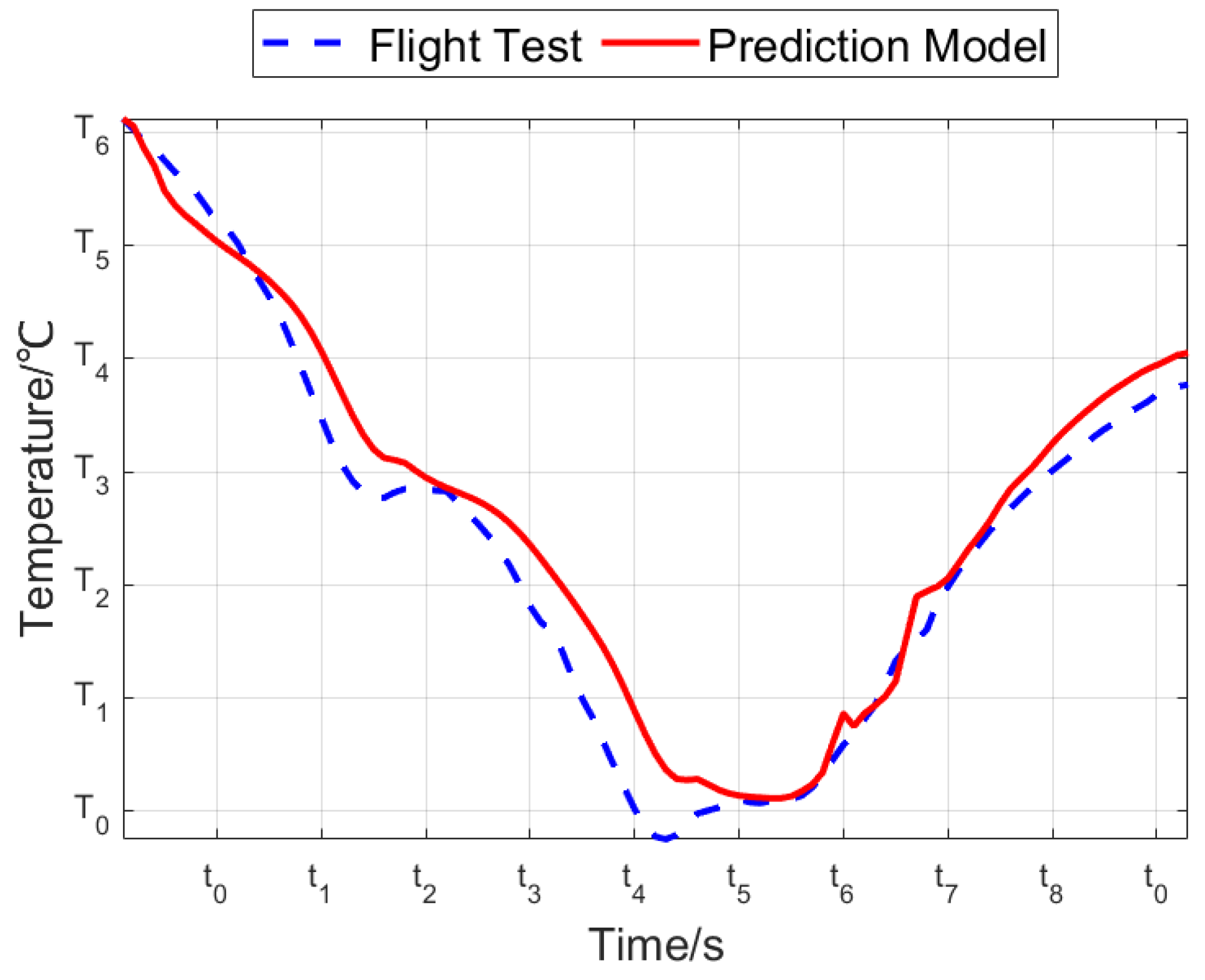
• The temperature environment prediction model established by the research fully considers the heat transfer relationship between the inside and outside of the aircraft cabin and the dynamic changes of the heat transfer coefficient. It can separate the trend change term from the constant term, eliminate the change lag phenomenon in the previous temperature environment prediction, and realize the accurate dynamic prediction of the temperature environment inside the aircraft cabin.
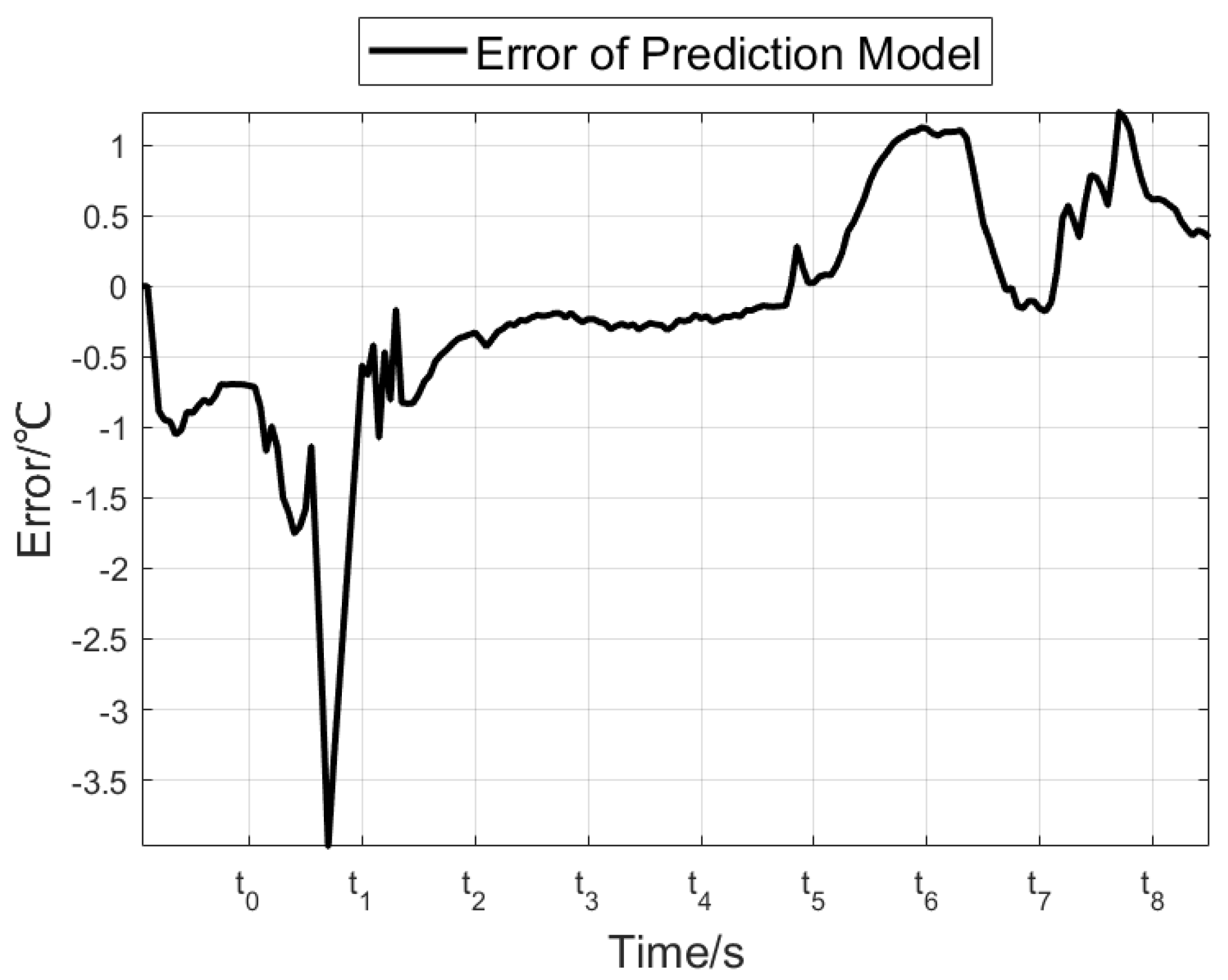
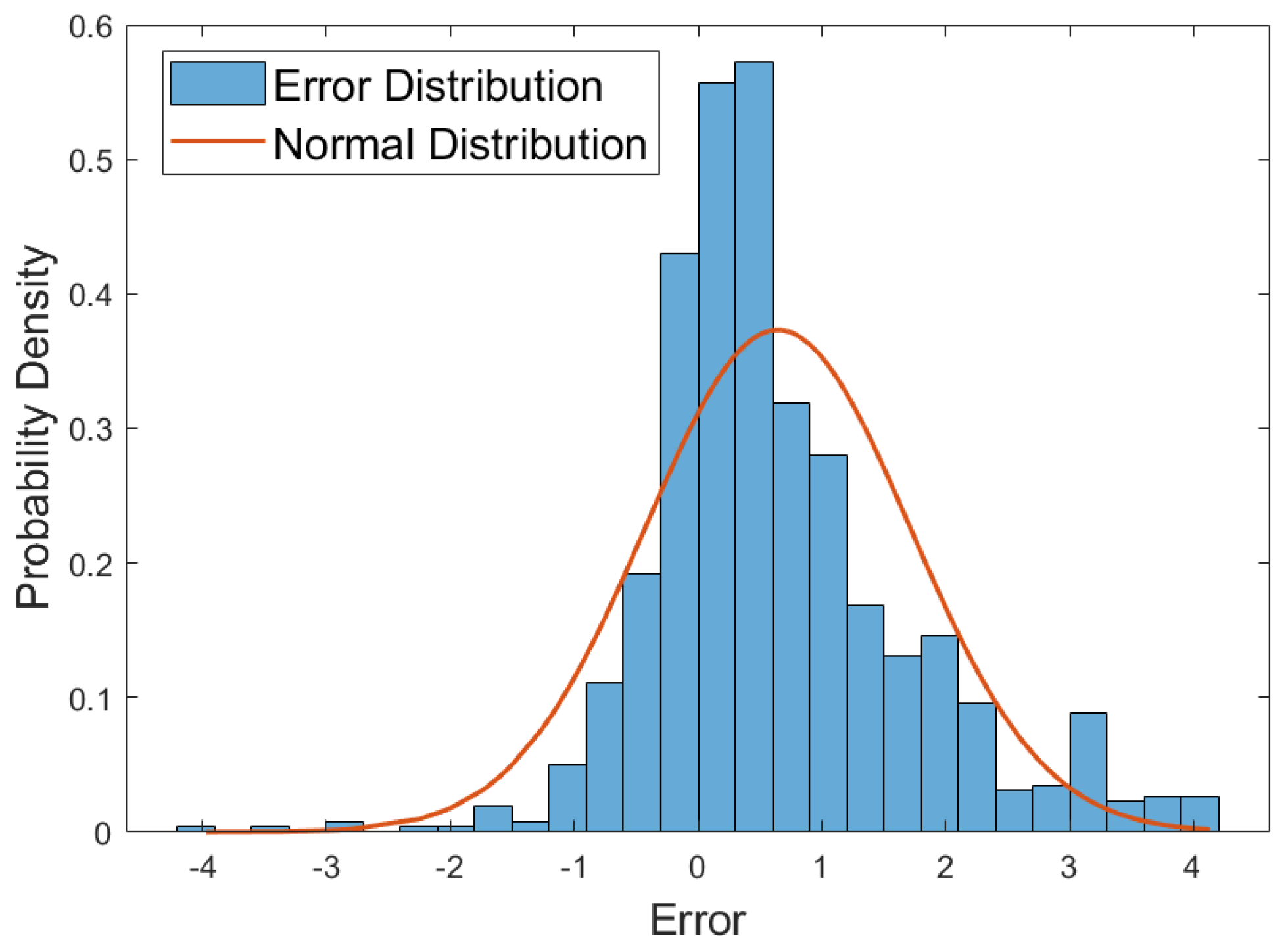
• The measured data of the cabin temperature environment of 16 flights of an aircraft show that the prediction accuracy of the established prediction model is good after extrapolation. The model predicts that the maximum error does not exceed 2.8 °C at a confidence level of 95%, and the maximum root mean square error is 2.4 °C.
• The established temperature prediction model can reflect the actual temperature environment experienced by the onboard equipment in the aircraft cabin during its service life. Practical engineering applications show that the temperature environment prediction model can effectively support thermal design optimization and the formulation of test conditions.
• The established temperature prediction model is solved based on the data of flight tests. Therefore, the model is only applicable to current aircraft and helps to optimize and verify the design of airborne equipment after the test flight. In the future, it is recommended to conduct actual temperature environment measurements on more aircraft models to obtain a temperature prediction model that is common to different structural configurations and to guide the formulation and verification of the temperature environment’s worth for the design requirements of similar or new aircraft.

References

1. Equipment Development Department of the Central Military Commission of Communist Party of China. Materiel Environment Engineering Terms; Publication and Distribution Department of Military Standards, GAD: Beijing, China, 2007. [Google Scholar]
2. Fu, Y.; Chang, H.J.; Wu, Y.Q.; Xue, H. Dynamic temperature predicted model for airplane platform based on measured data. Acta Aeronaut. Astronaut. Sin. 2014, 35, 2472–2480. [Google Scholar]
3. Sanchez, F.; Liscouet-Hanke, S. Thermal Risk Prediction Methodology for Conceptual Design of Aircraft Equipment Bays. Aerosp. Sci. Technol. 2020, 104, 105946. [Google Scholar] [CrossRef]
4. Sanchez, F.; Huzaifa, A.M.; Liscouet-Hanke, S. Ventilation Considerations for an Enhanced Thermal Risk Prediction in Aircraft Conceptual Design. Aerosp. Sci. Technol. 2021, 108, 106401. [Google Scholar] [CrossRef]
5. Li, H.; Zhang, J.J.; Fu, Y.; Shi, H.; Wan, J. Research on the Analysis and Prediction Method of Aircraft Temperature Environment in Severe Cold Areas. Environ. Technol. 2022, 40, 174–182. [Google Scholar]
6. Zhang, T.; He, Y.T.; Li, C.F.; Zhang, H.W.; Hou, B. Research on Local Temperature Environment of Ground Parking Aircraft. Acta Aeronaut. Astronaut. Sin. 2015, 36, 538–547. [Google Scholar]
7. Wang, T.; Wang, J. Ambient Temperature Flight Test of Airplane Nacelle and Analysis of Flight Result of One Aircraft. Mod. Mater. 2014, 1, 39–40. [Google Scholar]
8. Bao, S.; Wang, J.T.; Si, J.S.; Qi, C.W.; Chu, X.; Wang, C. Ambient Temperature Inside Liquid-cooled Electronic Pod. Equip. Environ. Eng. 2022, 19, 80–85. [Google Scholar]
9. Zhang, Y.H.; Shi, M.L. Analysis on Operating Temperature for Air-to-Air Missiles. Equip. Environ. Eng. 2015, 12, 99–103. [Google Scholar]
10. Li, D.P.; Zhu, P.P.; Chen, S.Q.; Pan, H.; Li, R.Q. Application of Linear Regression Analysis on Liquid Rocket Propellant Temperature Prediction. Missile Space Veh. 2020, 1, 43–47. [Google Scholar]
11. Zhao, S.Y.; Tian, R.L.; Wang, C.G.; Wang, W.J. Research on Environmental Conditions of Temperature and Humidity inside Container in Southeast Coast Region. Equip. Environ. Eng. 2007, 4, 44–47. [Google Scholar]
12. Li, H.B. BP Neural Network Prediction Method based on Temperature. Electron. Test 2013, 19, 62–64. [Google Scholar]
13. Li, H.; Zhang, J.J.; Fu, Y.; Xu, J.; Hao, Y.J. Research on Dynamic Prediction Method of Temperature Environment of Unmanned Aerial Vehicle Platform based on Physical Information and Neural Network. J. Phys. Conf. Ser. 2024, 2746, 012027. [Google Scholar] [CrossRef]
14. Lu, Y.; Zhang, J.J.; Fu, Y.; Liu, C. Seeker Cabin Temperature Prediction Based on Elman Neural Network in Airport Parking Conditions. Equip. Environ. Eng. 2020, 17, 21–26. [Google Scholar]
15. Fermin, U.J.; Benjamin, R.; Alain, D. Model Identification for Temperature Extrapolation in Aircraft Powerplant Systems. Int. J. Therm. Sci. 2013, 64, 162–177. [Google Scholar]
16. Ying, Z.; Wang, T.; Xiao, J.; Feng, X. Temperature Prediction of Electrical Equipment Based on Autoregressive Integrated Moving Average Model. In Proceedings of the 2017 32nd Youth Academic Annual Conference of Chinese Association of Automation (YAC), Hefei, China, 19–21 May 2017; pp. 197–200. [Google Scholar]
17. Yang, C.; Pang, L.P.; Wang, J.; Yue, Z.; Qu, H. Study on the Method of Thermal Prediction for Electronic Wing Pod Cabin. In Proceedings of the IECON 2017—43rd Annual Conference of the IEEE Industrial Electronics Society, Beijing, China, 29 October–1 November 2017. [Google Scholar]
18. Liu, R.; Song, J.; Luo, P.; Tian, F.; Li, W. Analysis and Prediction of Temperature of an Assembly Frame for Aircraft based on BP Neural Network. Int. J. Comput. Mater. Sci. Eng. 2023, 12, 2350006. [Google Scholar] [CrossRef]
19. Sheng, Z.Y.; Fu, S.; Wang, Y.P.; Qu, H.Q. Application of RVFL Neural Network in Temperature Prediction of Equipment cabin. China Sci. 2018, 13, 877–892. [Google Scholar]
20. Chen, G.Y.; Yang, S.; Peng, W.; Duo, L.L.; Zhang, J.P.; Liu, X.C. Transient Temperature Prediction Method for Spacecraft Using Process Neural Network. Spacecr. Eng. 2023, 32, 25–30. [Google Scholar]
21. Xia, Q.; Qiu, S.; Liu, X.Y.; Liu, M.; Guo, J.S.; Lin, X.H. Data-driven based Approach for Intelligent Temperature Forecasting of in-orbit Satellites. Syst. Eng. Ang Electron. 2024, 46, 1619–1627. [Google Scholar]
22. Mahulikar, S.P.; Kolhe, P.S.; Rao, G.A. Skin-Temperature Prediction of Aircraft Rear Fuselage with Multimode Thermal Model. J. Thermophys. Heat Transf. 2005, 19, 114–124. [Google Scholar] [CrossRef]
23. Zhang, Q. Calculation of Transient Heat Load for Aircraft Cabins. Master’s Thesis, Nanjing University of Aeronautics and Astronautics, Nanjing, China, 2009. [Google Scholar]
24. Luo, C.; Wan, J.; Ding, C.; Sun, Y.S. Predicting Method of Missile Storage Temperature Based on Thermal Network Model. Equip. Environ. Eng. 2017, 14, 89–92. [Google Scholar]
25. Pang, L.P.; Zhao, M.; Luo, K.; Yin, Y.; Yue, Z. Dynamic Temperature Prediction of Electronic Equipment under High Altitude Long Endurance Conditions. Chin. J. Aeronaut. 2018, 31, 1189–1197. [Google Scholar] [CrossRef]
26. Li, H.; Zhang, J.; Fu, Y.; Hao, Y.; Xu, J.; Zhong, Y. Research on Data-Driven Integrated Environment Prediction Method for the Typical Cabin of Helicopter. In Proceedings of the 2023 Global Reliability and Prognostics and Health Management Conference (PHM-Hangzhou), Hangzhou, China, 12–15 October 2023; pp. 1–6. [Google Scholar]
27. Lv, Y.G.; Ren, G.J.; Liu, Z.X.; Kang, Z. Thermal Analysis of Fuel Tank for Aircraft. J. Propuls. Technol. 2015, 36, 61–67. [Google Scholar]
28. Chen, Y.L.; Zhu, J.Z.; Chen, T.M.; Zhu, C.C.; Wei, P.T.; Xu, Y.Q. Study on Operating Temperature Prediction Model of Aero High-speed Gears. J. Mech. Transm. 2024, 48, 1–9. [Google Scholar]
29. Yin, J.B.; Wang, S.S.; Hou, X.; Hou, X.; Wang, Z.X.; Xu, Z. Transient Prediction Model of Finned Tube Storage Energy System based on Thermal network. Appl. Energy 2023, 38, 2395–2406. [Google Scholar] [CrossRef]
30. Liang, P.; He, T.; Liang, L.; Jiao, N.; Liu, W. Analytical Thermal Model of Slot for Electric Propulsion Motor in Electric Aircraft. IEEE Trans. Energy Convers. 2023, 38, 2662–2670. [Google Scholar] [CrossRef]
31. Yang, D. A Research on Design and Application of Kalman Filter. Master’s Thesis, Xiangtan University, Xiangtan, China, 2015. [Google Scholar]
32. Chen, T.T. Comparative Study of Cluster Analysis Method. Math. Comput. 2018, 7, 24–29. [Google Scholar]
33. Equipment Development Department of the Central Military Commission of Communist Party of China. Reliability Testing for Qualification and Production Acceptance; Publication and Distribution Department of Military Standards, GAD: Beijing, China, 2009. [Google Scholar]
34. Xia, L.L. Research on the Calculation of Transient Heat Load of Aircraft Cabins. Master’s Thesis, Nanjing University of Aeronautics and Astronautics, Nanjing, China, 2010. [Google Scholar]
35. Yang, S.M.; Tao, W.Q.B. Heat Transfer, 4th ed.; Higher Education Press: Beijing, China, 2006; p. 212. [Google Scholar]
36. Wang, X.Y. Fundamentals of Gas Dynamics, 1st ed.; Northwestern Polytechnical University Press: Xi’an, China, 2006; p. 111. [Google Scholar]
37. International Organization for Standard. Standard Atmosphere; ISO: Geneva, Switzerland, 1975. [Google Scholar]
38. Commission of Science, Technology and Industry for National Defense. Climatic Extremes for Military Equipment; Publication and Distribution Department of Military Standards, COSTIND: Beijing, China, 1991. [Google Scholar]
Figure 1. Schematic diagram of the structure of the study area (Zone 1).
Aerospace 11 00755 g001
Figure 2. Flight profile A.
Aerospace 11 00755 g002
Figure 3. Prediction results of internal temperature for cabin in flight profile A.
Aerospace 11 00755 g003
Figure 4. Prediction error of internal temperature for cabin in flight profile A.
Aerospace 11 00755 g004
Figure 5. Prediction results of internal temperature for cabin in flight profile B.
Aerospace 11 00755 g005
Figure 6. Prediction error of internal temperature for cabin in flight profile B.
Aerospace 11 00755 g006
Figure 7. Prediction results of internal temperature for cabin in flight profile C.
Aerospace 11 00755 g007
Figure 8. Prediction error of internal temperature for cabin in flight profile C.
Aerospace 11 00755 g008
Figure 9. Prediction results of internal temperature for cabin in flight profile D.
Aerospace 11 00755 g009
Figure 10. Prediction error of internal temperature for cabin in flight profile D.
Aerospace 11 00755 g010
Figure 11. Histogram of prediction model error distribution.
Aerospace 11 00755 g011
Figure 12. The severity of high temperature environmental conditions for a specific aircraft (schematic diagram).
Aerospace 11 00755 g012
Figure 13. The comparison of reliability test profiles.
Aerospace 11 00755 g013