Autonomous Dogfight Decision-Making for Air Combat Based on Reinforcement Learning with Automatic Opponent Sampling

Abstract

The field of autonomous air combat has witnessed a surge in interest propelled by the rapid progress of artificial intelligence technology. A persistent challenge within this domain pertains to autonomous decision-making for dogfighting, especially when dealing with intricate, high-fidelity nonlinear aircraft dynamic models and insufficient information. In response to this challenge, this paper introduces reinforcement learning (RL) to train maneuvering strategies. In the context of RL for dogfighting, the method by which opponents are sampled assumes significance in determining the efficacy of training. Consequently, this paper proposes a novel automatic opponent sampling (AOS)-based RL framework where proximal policy optimization (PPO) is applied. This approach encompasses three pivotal components: a phased opponent policy pool with simulated annealing (SA)-inspired curriculum learning, an SA-inspired Boltzmann Meta-Solver, and a Gate Function based on the sliding window. The training outcomes demonstrate that this improved PPO algorithm with an AOS framework outperforms existing reinforcement learning methods such as the soft actor–critic (SAC) algorithm and the PPO algorithm with prioritized fictitious self-play (PFSP). Moreover, during testing scenarios, the trained maneuvering policy displays remarkable adaptability when confronted with a diverse array of opponents. This research signifies a substantial stride towards the realization of robust autonomous maneuvering decision systems in the context of modern air combat.

1. Introduction

Autonomous air-to-air confrontation will be one of the most important forms of combat in future aerial warfare [1,2,3,4]. As far as we know, confrontation decision-making [5,6,7,8,9] and precise manipulation of autonomous aircraft [10,11,12] are two key technologies that are crucial for aerial combat tactical generation and execution. The autonomous dogfight maneuver decision-making technique is the integration of these two aspects. The primary objective in dogfighting is to formulate effective strategies for engaging opponents with precision weaponry. Dogfights are characterized by their lightning-fast pace and high maneuverability. Moreover, the constraints imposed by the engagement zone introduce another layer of complexity to the development of an effective maneuvering policy. Additionally, the strategies and maneuverability of opponents are various. Hence, it is still crucial to study dogfight maneuver decision-making for higher performance and robustness.

Diverse approaches have emerged to tackle the challenge of autonomous maneuvering decisions in dogfights [10,13]. On the one hand, optimal control methods, leveraging the theory of differential game models, have been employed to govern fighter aircraft during dogfights, albeit with certain idealized assumptions [14]. These approaches can be further categorized into analytical methods [15,16] and numerical methods [17,18]. On the other hand, planning and optimization strategies have been explored as a means to address dogfight maneuver decision-making, such as the pigeon-inspired optimization method [1] and the look-ahead search method [19]. Additionally, some rule-based autonomous decision-making methods have also been introduced, such as the fuzzy reasoning method [20] and the state–event–condition–action method [21]. More recently, the successful application of reinforcement learning (RL) in various confrontations [22,23,24,25] has ignited growing interest in its potential application to autonomous dogfighting. Previous studies [26,27] have showcased that RL methods offer several advantages in the realm of autonomous dogfight maneuvering decisions, including the ability to learn intricate dogfight maneuvering strategies, adaptability and generalization, and the ability to handle complex inputs. For example, the Hierarchical Soft Actor–Critic (SAC) RL method has demonstrated promising performance, particularly when integrated with high-resolution nonlinear simulation models during events like the AlphaDogfight Trial [26].

Based on the aforementioned review, it has been discerned that model-based methodologies [15,18] encounter significant limitations. Specifically, due to the inherent complexity of fighter aircraft, which possess six degrees of freedom (DOF) and exhibit highly coupled and nonlinear parameters, these model-based approaches are incapable of analytically deriving the optimal maneuvering actions. Additionally, they struggle to achieve real-time solutions for feasible tactical maneuvers through numerical techniques. Conversely, the RL methods [26,27,28,29] demonstrate a distinct advantage. By leveraging a vast number of trial-and-error iterations, the RL approach is capable of effectively discerning and learning the intricate relationships between real-time observations and the corresponding most appropriate maneuvering actions, thus demonstrating better decision-making capabilities. During the RL training process, the complexity of an agent’s policy dynamically adjusts in response to the actions of its opponents. Consequently, the opponent’s policy assumes a pivotal role in influencing the effectiveness of training. The thoughtful selection or design of the opponent’s policies takes on critical importance. This challenge is commonly referred to as the ’opponent sampling’ problem [30]. To address this issue, various self-play methods have been employed, including fictitious self-play [31,32], prioritized fictitious self-play (PFSP) [24], and Policy Space Response Oracles (PSRO) [33]. However, for a dogfight scenario, these methods may suffer from improving the learned maneuvering strategies efficiently. Motivated by the insights mentioned before, this work introduces an automatic opponent sampling framework to improve the proximal policy optimization (PPO) reinforcement learning algorithm for dogfight maneuvering decision-making, known as AOS-PPO, by borrowing concepts from PSRO.

The primary contribution of this research lies in the development and training of a novel automatic-opponent-sampling-based PPO algorithm. The proposed automatic opponent sampling framework, rooted in the principles of the PSRO, comprises three key components: the phased opponent policy pool, the Meta-Solver, and the Gate Function. The phased opponent policy pool and the Gate Function are designed to provide changing opponents, to avoid overfitting and improve the training performance. The Meta-Solver is designed to select an appropriate opponent from the opponent policy pool for efficient training. This work encompasses three contributions:

• Compared to the general RL framework [34,35], this study improves the performance of the PPO method in dogfight scenarios by introducing an automatic-opponent-sampling-based RL framework. Better dogfight maneuvers are generated using this improved PPO.
• Different from previous learning-based works, where the opponent is a fixed strategy [27] or historical learned policy [26], this work provides a standard approach which combines curriculum learning and self-play to adjust the opponent automatically for efficient learning.
• A dogfight maneuvering policy is trained within a simulation environment featuring nonlinear aircraft dynamics. The trained policy undergoes rigorous testing against various opponents [21,27], enabling a comprehensive analysis of its performance and adaptability.

This paper is organized as follows: Section 2 gives the reinforcement learning formulation for the dogfight scenario. Section 3 presents an improved PPO algorithm with the automatic opponent sampling framework. Results are provided in Section 4, and Section 5 concludes.

2. Problem Statement

This section mainly introduces the dogfight scenario studied in this work, and formulates the reinforcement learning for dogfight decision-making based on the Partially Observable Markov Decision Process (POMDP).

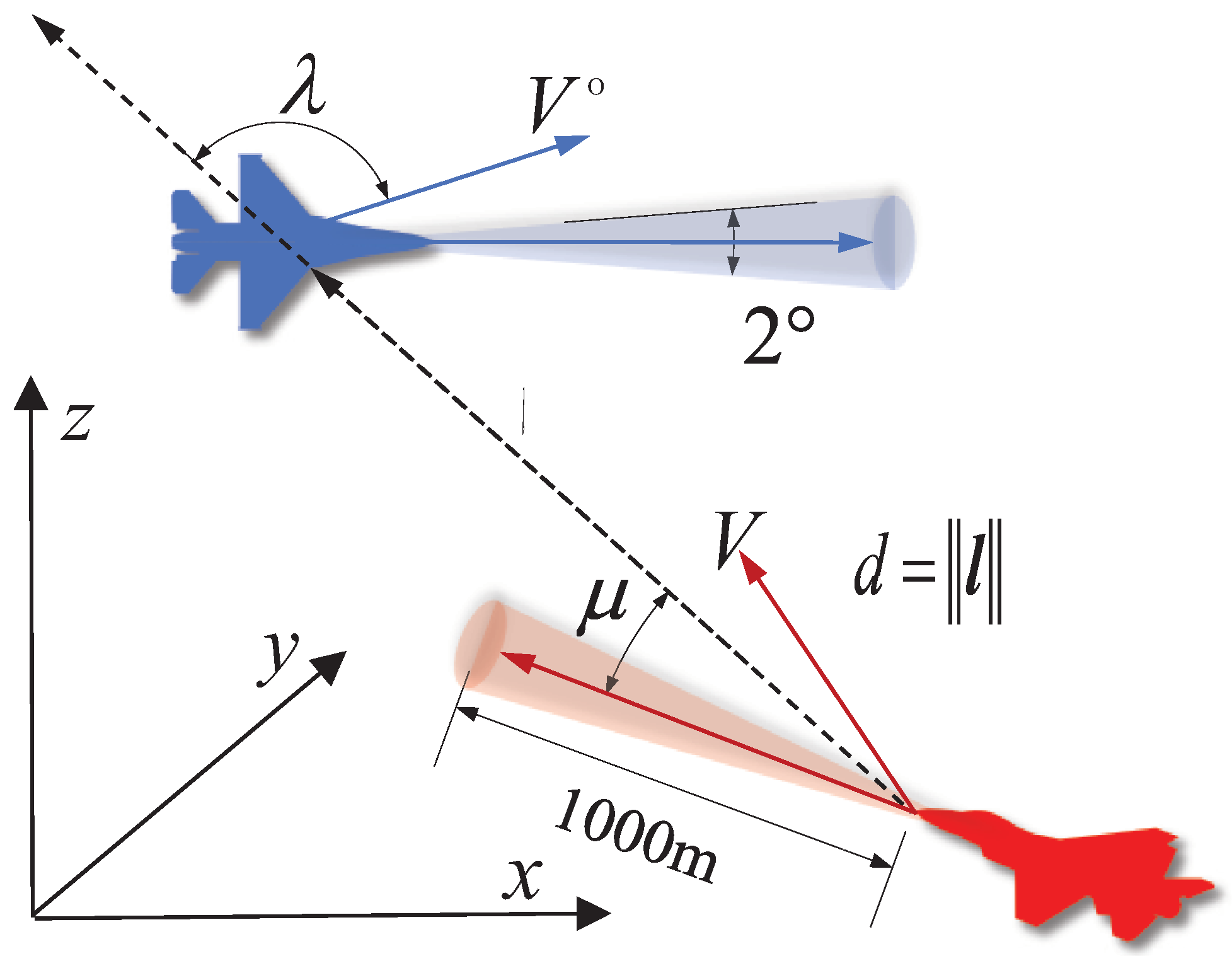
2.1. Dogfight Scenario

In this paper, as depicted in Figure 1, we employ a dogfight simulation environment integrating a six-degrees-of-freedom (6-DOF) nonlinear aircraft model along with a simulated flight controller. The dynamic function is defined as follows:

$$\begin{array}{cc}\hfill m\dot{u}& =-m(wq-vr)+T_{h,V}+\overline{q}{S}_{\mathrm{ref}}{C}_{\mathrm{X}}-mgsin\vartheta \hfill \\ \hfill m\dot{v}& =-m(ur-wp)+\overline{q}{S}_{\mathrm{ref}}{C}_{\mathrm{Y}}+mgsin\varphi cos\vartheta \hfill \\ \hfill m\dot{w}& =-m(vp-uq)+\overline{q}{S}_{\mathrm{ref}}{C}_{\mathrm{Z}}+mgcos\varphi sin\vartheta \hfill \\ \hfill I_{\mathrm{xx}}\dot{p}& =\left(I_{\mathrm{yy}}-I_{\mathrm{zz}}\right)qr+I_{\mathrm{xz}}(\dot{r}+pq)+\overline{q}{S}_{\mathrm{ref}}b{C}_{\mathrm{L}}\hfill \\ \hfill I_{\mathrm{yy}}\dot{q}& =\left(I_{\mathrm{zz}}-I_{\mathrm{xx}}\right)rp+I_{\mathrm{xz}}\left(r^2-p^2\right)+\overline{q}{S}_{\mathrm{ref}}b{C}_{\mathrm{M}}\hfill \\ \hfill I_{\mathrm{zz}}\dot{r}& =\left(I_{\mathrm{xx}}-I_{\mathrm{yy}}\right)pq+I_{\mathrm{xz}}(\dot{p}-qr)+\overline{q}{S}_{\mathrm{ref}}b{C}_{\mathrm{N}}\hfill \\ \hfill \dot{\varphi }& =p+tan\vartheta (qsin\varphi +rcos\varphi )\hfill \\ \hfill \dot{\theta }& =qcos\varphi -rsin\varphi \hfill \\ \hfill \dot{\psi }& =(qsin\varphi +rcos\varphi )/cos\vartheta \hfill \end{array}$$

(1)

where $\overline{q}={\displaystyle \frac{1}{2}}\rho V^2$ is the aerodynamic pressure. The $S_{\mathrm{ref}},b$ are, respectively, the wing area and wing span of the fighter aircraft. The ${[u,v,w]}^{\mathrm{T}}$ is the velocity vector in the body frame, and the position vector in the reference frame can be solved from ${[{\dot{x}}_{\mathrm{r}},{\dot{y}}_{\mathrm{r}},{\dot{z}}_{\mathrm{r}}]}^{\mathrm{T}}=C_b^r{[u,v,w]}^{\mathrm{T}}$. The aerodynamic coefficients $C_{\mathrm{X}},C_{\mathrm{Y}},C_{\mathrm{Z}}$, the aerodynamic moment coefficients $C_{\mathrm{L}},C_{\mathrm{M}},C_{\mathrm{N}}$, and the thrust function $T_{h,V}$ are based on the data of an F-16 fighter in nominal flight conditions, which is presented in book [36]. The critical angle of attack and maximum indicated airspeed of the fighter model are, respectively, ${30}^{°}$ and 420 m/s. Moreover, the flight controller is designed as shown in book [36]. Building upon the fighter aircraft model, our analysis considers a three-dimensional dogfight engagement scenario involving two fighters, both of which are striving to target the other fighter, as depicted in Figure 2. Here, d represents the relative range, while $\mu$ and $\lambda$ denote the fighter antenna train angle (ATA) and the opponent’s aspect angle (AA) relative to the line of sight (LOS).

The primary objective of dogfight decision-making is to orient the fighter toward the opponent for a weapons lock that can be modeled as the Weapons Engagement Zone (WEZ) [26]. Visualized in Figure 2, the mathematical expression of the WEZ is defined as follows:

$$d_{min}\le d\le 1000m,\mu \le 1°$$

(2)

where $d_{min}$ is the minimum shooting distance of 100 m. In this investigation, once these constraints are met, the fighter can achieve a shot. Additionally, it is worth noting that the longer the shooting duration, the greater the damage inflicted on the opponent. Consequently, the computational formula of the health point (HP) is defined as follows:

$$\mathrm{HP}\left(t\right)=\mathrm{HP}\left(t\right)-{\displaystyle \frac{1000-d}{900}}\Delta t$$

(3)

where $\Delta t$ denotes the simulation step time.

2.2. POMDP Formulation

The autonomous dogfight maneuvering decision can be modeled as a sequential decision-making problem with the mathematical formalism of the Partially Observable Markov Decision Process (POMDP). A POMDP comprises a set of states S, a set of observations O, a set of actions A, a transition function T, and a reward function R, forming a tuple $〈S,O,A,T,R〉$. The decision goal is to find the optimal policy ${\pi }^{*}$ that provides the highest cumulative rewards:

$$V_{\pi }\left(s\right)=E_{\pi }\left\{\sum _{t=0}^{t_{\mathrm{f}}}{\gamma }^{t-1}{r}_t\mid s_0=s\right\},{\pi }^{*}=\underset{\pi }{argmax}{V}_{\pi }\left(s\right)$$

(4)

where $\gamma$ represents the discount factor. The value function $V_{\pi }\left(s\right)$ is the anticipated future return at state s given a policy $\pi$. The variable $t_{\mathrm{f}}$ denotes the number of steps in the POMDP. Another crucial concept related to expected cumulative rewards is the action value function, a fundamental component in most RL algorithms. It is defined as follows:

$$Q_{\pi }(s,a)=E_{\pi }\left\{\sum _{t=0}^{t_{\mathrm{f}}}{\gamma }^{t-1}{r}_t\mid s_0=s,a_0=a\right\}$$

(5)

In this context, the optimal policy can be determined by estimating the Q-function. In this study, the components of the POMDP are as follows:

2.2.1. State, Observation, and Action

The state set for dogfight maneuvering decisions comprises the flight parameters of both the agent and its opponent, along with data pertaining to their relative movements. The observations utilized in this study are detailed in

Table 1. The set of observations in dogfights.

Observations	Meaning
$V_{\mathrm{ias}}$	Agent’s indicated airspeed (IAS)
V	Agent’s velocity in the reference frame
$V^{\mathrm{o}}$	Opponent’s velocity in the reference frame
$\alpha$	Agent’s angle of attack
$\varphi$	Agent’s rolling angle
$\vartheta$	Agent’s pitching angle
$\psi$	Agent’s yawing angle
d	Relative range between two fighters
$\dot{d}$	Closing rate of the opponent
h	Agent’s altitude
$h_{\mathrm{op}}$	Opponent’s altitude
$\mu$	Agent’s antenna train angle
$\lambda$	Opponent’s aspect angle

and can be obtained from a variety of sources, including airspeed indicators, inertial measurement units, onboard radar systems, airborne warning and control (AWACS) aircraft, and others. The actions are defined in

Table 2. Actions in dogfight maneuvering decision.

Action	Value Range	Meaning
$T^{\mathrm{cmd}}$	$0\%\sim 100\%$	Throttle command
$n_z^{\mathrm{cmd}}$	−$30 {\mathrm{m/s}}^2$∼ $90 {\mathrm{m/s}}^2$	Normal acceleration command
$n_y^{\mathrm{cmd}}$	−$30 {\mathrm{m/s}}^2$∼ $30 {\mathrm{m/s}}^2$	Lateral acceleration command
${\omega }_x^{\mathrm{cmd}}$	−4 rad/s ∼ 4 rad/s	Roll rate command

.

2.2.2. Reward

Success in the dogfight depends on achieving a narrow pointing angle and maintaining close range to the opponent. This poses a significant challenge during the RL training, so the reward function is defined as follows:

$$r_t=r_{\mathrm{ep}}+{\lambda }_r{r}_{\mathrm{s}}$$

(6)

where $r_{\mathrm{ep}}$ is the episodic reward. It takes a value of 100 when the agent wins, a value of −100 when the agent crashes, and a value of 0 otherwise. ${\lambda }_r$ represents the weight of the shaped reward $r_{\mathrm{s}}$, which decays during training to avoid too much interference from the handcrafted reward on policy learning. The $r_{\mathrm{s}}$ is given by the following:

$$\begin{array}{c}\hfill r_{\mathrm{s}}=r_{\mathrm{aim}}+r_{\mathrm{geo}}+r_{\mathrm{close}}+r_{\mathrm{gun}}+r_{\mathrm{def}}+r_{\mathrm{alt}}+r_{\mathrm{collision}}\end{array}$$

(7)

It is advantageous to define derivatives of the reward function for different state ranges. Hence, an exponential potential function [37] is introduced:

$$L(\varpi ,x,x_{\mathrm{m}})={\displaystyle \frac{1-e^{-\varpi (x-x_{\mathrm{m}})}}{1+e^{-\varpi (x-x_{\mathrm{m}})}}}$$

(8)

where $\varpi$ is a rate parameter that has different values for different variables and $x_{\mathrm{m}}$ is the mean value of the x. The value range of this function is [0, 1], and it is monotonically increasing. Based on this function, mathematical definitions of the shaped reward function components [26] are as follows:

(1) Aiming reward $r_{\mathrm{aim}}$: It is used to reward the agent to aim at the opponent. It is given by the following:

$$r_{\mathrm{aim}}=0.8\times \left({\left({\displaystyle \frac{\mu }{\pi }}\right)}^2+{\left({\varphi }_e\right)}^2\right)$$

(9)

where ${\varphi }_e$ represents the angle of the LOS vector with respect to the fighter’s lifting plane. This reward can encourage the agent to include the opponent in the lifting plane and achieve fast targeting [38]. It is computed as follows:

$${\varphi }_{\mathrm{e}}={\displaystyle \frac{1}{\pi }}{cos}^{-1}{\displaystyle \frac{{\mathit{e}}^L·{\mathit{l}}_{\mathrm{p}}^{\mathrm{W}}}{∥{\mathit{e}}^L∥·∥{\mathit{l}}_{\mathrm{p}}^{\mathrm{W}}∥}},{\mathit{l}}_{\mathrm{p}}^{\mathrm{W}}=\left[1,0,0\right]·{\mathit{l}}^{\mathrm{W}}$$

(10)

where the ${\mathit{e}}^L$ is the unit vector of the fighter lift and the ${\mathit{l}}^{\mathrm{W}}$ is the LOS vector in the wind frame.

(2) Geometry reward $r_{\mathrm{geo}}$: It is used to reward the agent for attaining the tail chase geometry ($\mu =0,\lambda =0$). It also penalizes the agent for allowing its opponent to do the same ($\mu =\pi ,\lambda =\pi$). It is given by the following:

$$r_{\mathrm{geo}}=\left({\displaystyle \frac{\mu }{\pi }}-2\right)\times L\left(18,{\displaystyle \frac{\lambda }{\pi }},0.5\right)-{\displaystyle \frac{\mu }{\pi }}+1$$

(11)

(3) Relative position $r_{\mathrm{close}}$: The agent receives a reward when it approaches its opponent and a penalty when it does the opposite. However, as the relative distance converges to 0 or the opponent’s aspect angle converges to $\pi$, the reward should also converge to 0. Therefore, $r_{\mathrm{close}}$ is defined as follows:

$$r_{\mathrm{close}}={\displaystyle \frac{-\dot{d}}{500}}\times \left(1-L\left(18,{\displaystyle \frac{\lambda }{\pi }},0.5\right)\right)\times L\left({\displaystyle \frac{1}{500}},d,900\right)$$

(12)

(4) Shooting reward $r_{\mathrm{gun}}$: The agent can receive a reward when it achieves the shooting opportunity (100 m ≤ d ≤ 1000 m, $\mu \le 1°$). Furthermore, the agent should receive a high shooting reward when it is close to its opponents with high damage (e.g., 300 < d < 900 m). However, when the opponent is close enough (e.g., d < 650 m), shooting rewards should decrease as the distance increases to discourage overshooting. Hence, the shooting reward $r_{\mathrm{gun}}$ is defined as follows:

$$r_{\mathrm{gun}}={\Gamma }_{\mathrm{gun}}\times \left(1-L\left(1000,{\displaystyle \frac{\mu }{\pi }},{\displaystyle \frac{1}{180}}\right)\right)$$

(13)

where ${\Gamma }_{\mathrm{gun}}$ is the range factor that determines the distances at which $r_{\mathrm{gun}}$ has the greatest magnitude. It is defined as follows:

$${\Gamma }_{\mathrm{gun}}=\left\{\begin{array}{c}{D}_{\mathrm{gun}}\times L\left(0.01,d,300\right)\mathrm{if}d<650\hfill \\ D_{\mathrm{gun}}\times \left(1-L\left(0.01,d,900\right)\right)\mathrm{else}\hfill \end{array}\right.$$

(14)

where

$$D_{\mathrm{gun}}=\left\{\begin{array}{c}2\times \left(1+{\displaystyle \frac{900-d}{600}}\right)\mathrm{if}300<d<900\hfill \\ 2\mathrm{else}\hfill \end{array}\right.$$

(15)

(5) Defense reward $r_{\mathrm{def}}$: It is used to penalize the agent when its opponent achieves a shooting opportunity. Similarly to the shooting reward, it is given by the following:

$$r_{\mathrm{def}}={\Gamma }_{\mathrm{def}}\times L\left(800,{\displaystyle \frac{\lambda }{\pi }},{\displaystyle \frac{179}{180}}\right)$$

(16)

where

$${\Gamma }_{\mathrm{def}}=\left\{\begin{array}{c}{D}_{\mathrm{def}}\times L\left(0.02,d,100\right)\mathrm{if}d<750\hfill \\ D_{\mathrm{def}}\times \left(1-L\left(0.01,d,750\right)\right)\mathrm{else}\hfill \end{array}\right.$$

(17)

where

$$D_{\mathrm{def}}=\left\{\begin{array}{c}-2\times \left(1+{\displaystyle \frac{1500-d}{1400}}\right)\mathrm{if}100<d<1500\hfill \\ -2\mathrm{else}\hfill \end{array}\right.$$

(18)

(6) Altitude reward $r_{\mathrm{alt}}$: The agent should be penalized when it is at low altitude (around 500m) to prevent it from crashing. It is defined as follows:

$$r_{\mathrm{alt}}=-3.5\times \left(1-L\left(0.05,h,500\right)\right)$$

(19)

(7) Collision reward $r_{\mathrm{collision}}$: It is used to penalize the agent for violating a minimum distance threshold when pursuing, which may lead to collision or overshooting. It is given by the following:

$$r_{\mathrm{collision}}=-L\left(18,{\displaystyle \frac{\lambda }{\pi }},0.5\right)\times \left(1-L\left(0.02,d,270\right)\right)$$

(20)

3. AOS-PPO Algorithm

In the RL training paradigm, the selection of an appropriate opponent plays a crucial role in enhancing the training efficacy. Specifically, during the initial phase of training, an overly formidable opponent can impede the agent’s ability to explore effective strategies. Conversely, in the latter stage of training, an overly feeble opponent may lead to a degradation in the decision-making performance of the learned strategies. Consequently, this study presents an automatic opponent sampling (AOS) method and employs the proximal policy optimization (PPO) RL algorithm for training dogfight maneuvering strategies. This section systematically elaborates on the theoretical foundation of the AOS method, the framework of AOS, the components constituting AOS, and the AOS-PPO algorithm implemented within the distributed training framework.

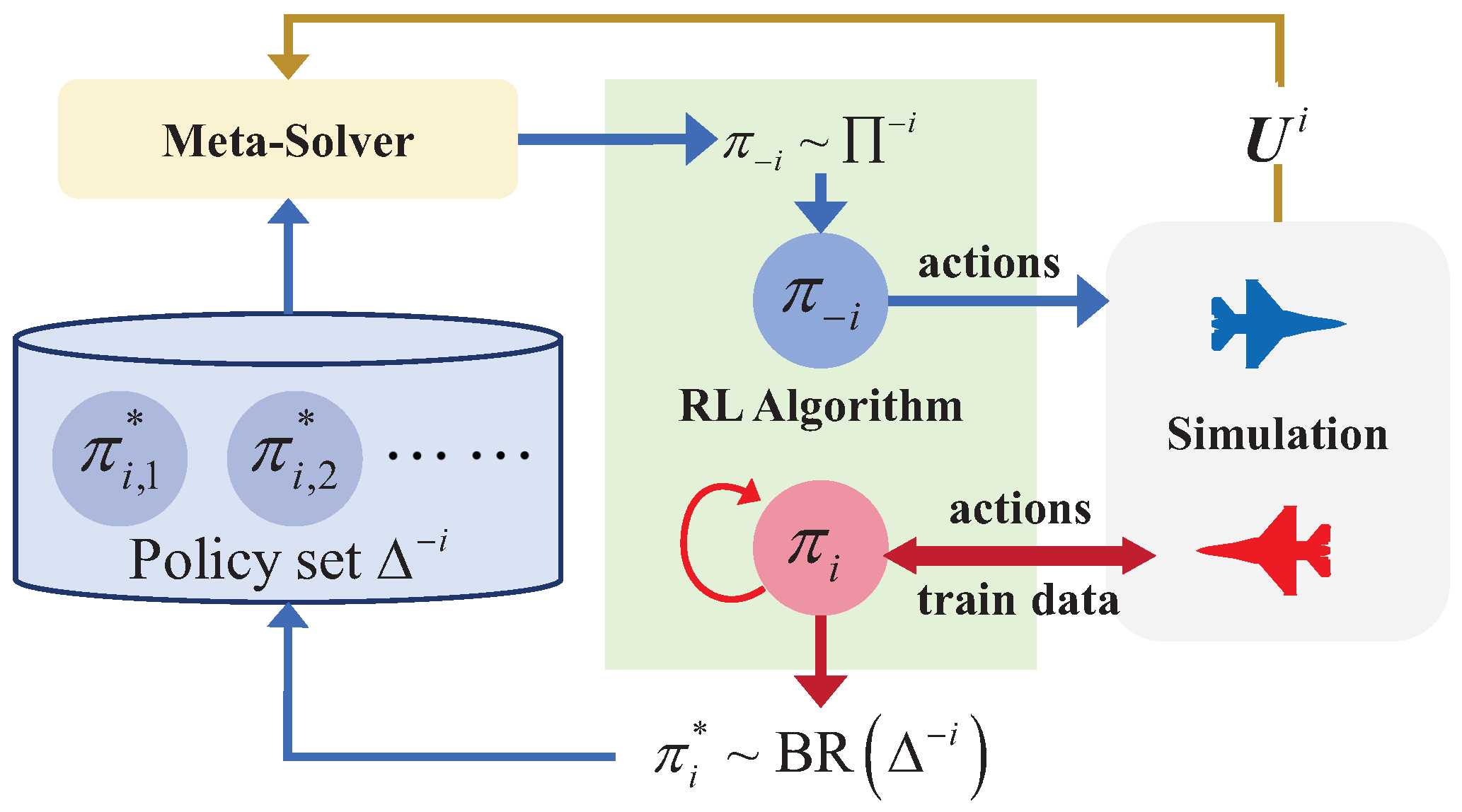
3.1. Self-Play Methods

Self-play is a typical opponent sampling method which originates from the solution of game strategies based on the Nash equilibrium. Consider a game G with N agents. In the context of a dogfight game, for instance, $N=2$. The strategies of all agents constitute the strategy set $\mathcal{P}=\left\{{\pi }^1,\dots ,{\pi }^i,\dots ,{\pi }^N\right\}$ of the game G. Each agent i maintains a strategy set ${\Delta }^i$ that encompasses all of its pure strategies. In the game G, the best response (BR) of a single agent i is given by

$$b^i\left({\pi }^{-i}\right)=arg\underset{{\pi }^i\in {\Delta }^i}{max}R({\pi }^i,{\pi }^{-i})$$

(21)

where ${\pi }^{-i}$ denotes the strategies of all agents in the game strategy set $\mathcal{P}$ except agent i, and $R({\pi }^i,{\pi }^{-i})$ represents the expected return when agent i adopts the strategy ${\pi }^i$. The Nash equilibrium of the game G implies that all strategies in the game strategy set $\mathcal{P}$ are best responses, formally expressed as

$${\pi }^i\in b^i\left({\pi }^{-i}\right),\forall i\in N$$

(22)

Fictitious play (FP [39]) iteratively approximates the Nash equilibrium as agents alternately compute the best responses to opponents. In a symmetric two-player game with identical decision-making goals for both sides, such as in dogfighting, FP simplifies to self-play. Here, finding the best response to the opponent equals finding it against one’s own historical strategies. Therefore, fictitious self-play (FSP [31]) trains the opponent’s best response through reinforcement learning and uses supervised learning to train an opponent’s strategy to simulate the historical strategy set, which is equivalent to uniformly sampling opponents from the historical strategy set. Moreover, Neural Fictitious Self-Play (NFSP [32]) incorporates a deep neural network in the supervised learning part of FSP.

However, uniformly sampling from the agent’s entire historical strategy set ${\Delta }^i$ is computationally costly, and obsolete strategies are more likely to be sampled, potentially degrading reinforcement learning performance. Hence, $\sigma$-$\mathrm{uniform}$ self-play uniformly samples only some newly added strategies from ${\Delta }^i$, with a zero sampling probability for the rest. Priority fictitious self-play (PFSP [24]) samples, with higher probability, strategies in its own historical strategy set, against which the agent has a lower winning rate, enhancing reinforcement learning training. Furthermore, the Policy Space Response Oracle (PSRO [33]) is a method that can dynamically solve the probability distribution $\Pi$ to sample opponents from the historical strategy set, which is called the Meta-Solver. Moreover, in PFSP, the priority-based probability distribution of sampling opponents is also a kind of Meta-Solver. Within the PSRO, the payoffs for each policy of the agent playing against each strategy of its opponent can be calculated through simulations, forming the payoff matrix ${\mathit{U}}^i$. As depicted in Figure 3, during the agent’s update, the PSRO computes the $\Pi$ using a Meta-Solver based on the payoff matrix ${\mathit{U}}^i$ and samples the opponent’s strategies for RL training. Then, the PSRO uses RL to approximate the best response ${\pi }_i^{*}$, and adds it into the strategy set, extending the payoff matrix via simulations.

The above self-play methods can be summarized as follows: During the process of training the opponent’s best response in reinforcement learning, a rule is defined to collect opponent strategies from historical strategies to form an opponent strategy pool, and a probability distribution is defined to sample opponents from it. Therefore, based on the framework of the PSRO and drawing on the priority concept in PFSP, this paper proposes an automatic opponent sampling (AOS) method to improve the reinforcement learning for dogfighting.

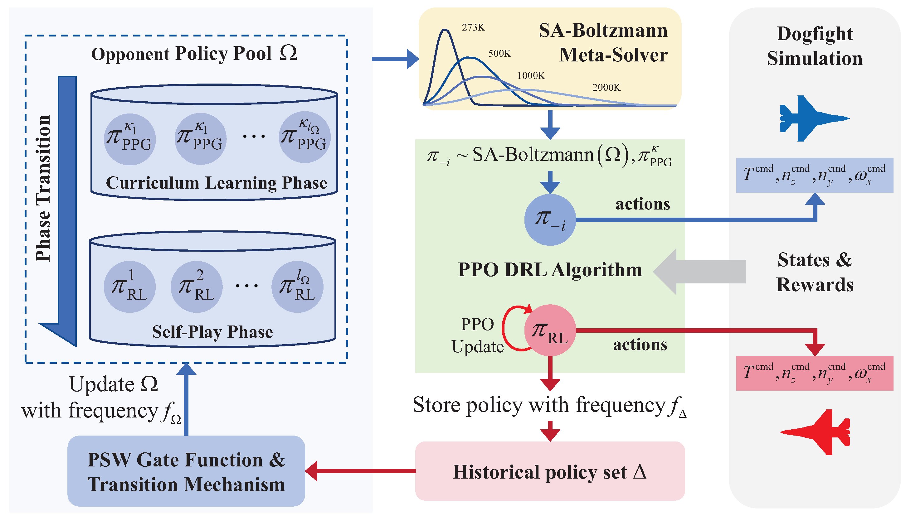
3.2. The Framework of AOS

In the context of training dogfight decisions, the PSRO suffers from low learning efficiency since using the RL algorithm to approximate the best response takes a long time in each iteration of the PSRO. Moreover, as the number of policies in $\Delta$ increases, the computation for simulations required to compute the $\mathit{U}$ also increases. Furthermore, if the opponent is sampled across the entire policy set, the stale policies are always selected, resulting in overfitting. Therefore, a novel automatic opponent sampling (AOS)-based RL framework is proposed to improve the training of dogfight maneuvering strategies. In this proposed AOS framework, the constraint of the best response in the PSRO is removed and a Gate Function [40] is introduced for updating the opponent policy pool.

As depicted in Figure 4, the opponent policy pool with a fixed length $l_{\Omega }$ is initialized with artificially designed strategies (curriculum learning phase). Compared with the PFSP and PSRO, AOS introduces an additional Gate Function to select strategies from the historical strategy set $\Delta$ at a fixed frequency $f_{\Omega }$, adding suitable strategies to the opponent policy pool and removing those that are not suitable as opponents for RL. Thus, as the training progresses, the opponent policy pool gradually transforms into historical strategies (self-play phase) obtained through RL training. The opponents for RL training are sampled from the opponent policy pool according to the Boltzmann probability distribution generated from the Meta-Solver inspired by the simulated annealing (SA) algorithm. Moreover, during the training process, the current strategy is stored at a fixed frequency $f_{\Delta }$ to form the historical strategy set $\Delta$.

3.3. The Components Constituting AOS

As shown in Figure 4, the AOS includes three key components: a phased opponent policy pool, an SA–Boltzmann Meta-Solver, and a priority sliding window (PSW) Gate Function. The phased opponent policy pool introduces the curriculum learning [41] technique to provide easy-to-hard opponents for RL training, improving the training efficiency. Moreover, the PSW Gate Function is designed to ensure that the strategies in the opponent’s policy pool $\Omega$ possess good decision-making performance, and to gradually shift the $\Omega$ from the curriculum learning phase to the self-play phase. In this way, it can prevent sampling opponents with low confrontation capabilities, which may cause interference and waste in the training process. Since the priorities of different opponent strategies need to be recalculated after the $\Omega$ is updated, unlike in PFSP, our Meta-Solver makes the probability distribution for sampling opponents gradually shift from a uniform distribution to a probability distribution that preferentially samples opponents with strong dogfighting capabilities. This ensures the balance between the diversity of opponents and high decision-making performance during the RL training process. The details of these components of the proposed AOS framework can be described as follows:

3.3.1. Phased Opponent Policy Pool

As illustrated in Figure 4, the strategies in the $\Omega$ are rooted in the historical policy set $\Delta$, which is a form of self-play. However, due to the relaxation of the BR constraint, in the early stages of training, policies in $\Delta$ possess poor knowledge about dogfight maneuvering, potentially impeding the efficiency of training. Furthermore, the opponents for early training should not have a strong dogfighting ability to avoid RL failing to yield positive rewards. To overcome these challenges, we propose the integration of curriculum learning within the opponent policy pool. This curriculum learning approach entails training the agent initially against simple opponents, which is progressively stronger, before engaging in self-play. Consequently, as illustrated in Figure 4, the opponent policy pool is divided into two phases: the curriculum learning (CL) phase and the self-play (SP) phase. Furthermore, the transition from the CL phase to the SP phase is not an abrupt shift, as elaborated upon in subsequent parts.

Within this curriculum learning, we draw inspiration from concepts such as slow cooling and probabilistic jumps, borrowed from the realm of simulated annealing (SA). These concepts inform the formulation of opponent strategies and the rules for sampling training data. During the CL phase, the $\Omega$ contains artificially designed strategies where the opponent’s actions include pursuit in a random direction with a decreasing probability. As illustrated in Figure 5 and Equation (23), through the decaying probability denoted as $\kappa$, the opponent’s policy steers the opponent to follow either a random vector ${\mathit{l}}_{\mathrm{r}}$ or the line-of-sight (LOS) vector $\mathit{l}$ based on the Pure Pursuit Guidance Law (PPG). This policy, combining elements of the random policy and the Pure Pursuit Guidance Law, is referred to as the ‘$\kappa$-PPG policy’ or ‘${\pi }_{\mathrm{PPG}}^{\kappa }$’ policy.

$${\mathit{l}}_{\mathrm{r}}=\left\{\begin{array}{c}\mathit{l}\mathrm{if}U(0,1)\ge \kappa \hfill \\ ∥l∥C_{\mathrm{r}}(0,{\vartheta }_{\mathrm{r}},{\psi }_{\mathrm{r}}){\mathit{i}}_V\mathrm{otherwise}\hfill \end{array}\right.$$

(23)

where

$$\kappa ={\left(0.98\right)}^{{\displaystyle \frac{N_{\mathrm{e}}}{20}}}\kappa ,{\vartheta }_{\mathrm{r}},{\psi }_{\mathrm{r}}=U(-{90}^{°},{90}^{°},2)$$

(24)

where U represents a random function following uniform distribution, and $N_{\mathrm{e}}$ stands for the total number of state transition trajectories throughout the learning process for each simulation process. Additionally, within each iteration of RL, the policy update is implemented with a probability $p_{\mathrm{SA}}$, which is also defined by the decreasing $\kappa$.

$$p_{\mathrm{SA}}=\left\{\begin{array}{c}1r_{e+1}^a\ge r_e^a\hfill \\ \kappa r_{e+1}^a<r_e^a\hfill \end{array}\right.$$

(25)

where $r_e^a$ represents the average reward of each learning epoch. If the current policy outperforms the previous policies, the transition trajectories sampled are used for updating the policy. Conversely, when the current policy is less effective, the samples are utilized with a probability determined by $\kappa$. Furthermore, the probability $\kappa$ has a lower limit as it decreases to ensure that trajectory samples with lower cumulative rewards can still contribute to policy exploration. The parameter $\kappa$ falls within the range of [0, 1]. When $\kappa$ equals 0, the agent is trained against a guidance-based opponent. Conversely, when $\kappa$ equals 1, the opponent policy adopts a randomized approach.

3.3.2. SA–Boltzmann Meta-Solver

Our Meta-Solver is a specially designed algorithm capable of generating an opponent policy sampling distribution with adjustable parameters. Drawing on our analysis of prior works [32,42], the uniform distribution can help ensure the diversity of opponents (e.g., $\sigma$-$\mathrm{uniform}$ self-play [42]), while it becomes increasingly beneficial to engage with opponents of higher skill levels as training progresses (e.g., PFSP [24]). To accommodate this, our Meta-Solver is devised to shift the sampled opponent policy from weaker to stronger in parallel with the RL training. This process is delineated in Algorithm 1. Within this algorithm, we incorporate the concept of ‘slow cooling’, a common feature in SA algorithms, into a Boltzmann distribution. The Boltzmann distribution, characterized by its maximum entropy probability distribution, ensures uniformity of sampling, particularly when opponent policies have different importance. It is defined as follows:

$$p_i={\displaystyle \frac{e^{{ϵ}_i/k_{\mathrm{b}}{T}_{\mathrm{b}}}}{{\sum }_{j=1}^l{e}^{{ϵ}_j/k_{\mathrm{b}}{T}_{\mathrm{b}}}}}$$

(26)

where $k_{\mathrm{b}}$ denotes the Boltzmann constant, and $T_{\mathrm{b}}$ signifies the ‘temperature’ of the opponent policy pool. ${ϵ}_i$ represents the opponent’s episode reward, which is defined by the win ratio (WR) as follows:

$${ϵ}_i=E_{\varsigma \sim {\pi }^i}\left[\mathrm{W}{\mathrm{R}}_{\varsigma }\left({\pi }^i\right)\left|{\pi }^i\in \Omega \right.\right],i\in l_{\Omega }$$

(27)

$$\mathrm{W}{\mathrm{R}}_{\varsigma }\left({\pi }^i\right)=\left\{\begin{array}{c}1\mathrm{if}{\pi }^i\mathrm{win}\hfill \\ 0\mathrm{else}\hfill \end{array}\right.$$

(28)

where $\varsigma$ is the transition trajectory in which the opponent uses policy ${\pi }^i$ among the simulation transition trajectories of the RL training process. Moreover, the ${ϵ}_i$ is initialized as 1 when ${\pi }^i$ has not been used in simulations. In our SA–Boltzmann Meta-Solver, $T_{\mathrm{b}}$ undergoes a gradual decay during the training process and is reset when the opponent policy pool is updated. When $T_{\mathrm{b}}$ is reset to a high value, the resulting sampling distribution closely resembles a uniform distribution. As $T_{\mathrm{b}}$ decreases to a lower value, policies with higher rewards are granted a greater probability of being sampled.

Algorithm 1 SA–Boltzmann Meta-Solver

1: Initialize ${{ϵ}_i}_{,i\in l_{\Omega }}=1$   2: Initialize the temperature $T_{\mathrm{b}}$   3: for training iteration times $k=1,\cdots ,K$ do   4:    sample opponent’s policy from $\Omega$ using Equation (26)   5:    do simulations for DRL training   6:    update ${{ϵ}_i}_{,i\in l}$ with samples from simulations   7:    if $k\%20=0$ and $k>0$ then   8:        $T_{\mathrm{b}}=0.98T_{\mathrm{b}}$   9:    end if 10:    if $\Omega$ updated then 11:       Reset $T_{\mathrm{b}}$ and ${{ϵ}_i}_{,i\in l_{\Omega }}=1$ 12:    end if 13: end for

3.3.3. Priority Sliding Window Gate Function

During the training progress, the trained policy is stored in the historical policy set $\Delta$ at a fixed frequency $f_{\Delta }$. As shown in Figure 6 and Algorithm 2, the Gate Function (GF) is defined using a priority sliding window (PSW), which is used to push the more new policy in $\Delta$ into the $\Omega$ and pop out the most old policy in $\Omega$. Moreover, the historical policy in $\Delta$ is pushed into $\Omega$ only when its win ratio exceeds 50%, indicating the priority in the PSW. It is noticed that the frequency $f_{\Delta }$ should be not smaller than the frequency of updating the $\Omega$ ($f_{\Omega }$). Additionally, the transition of two phases of the opponent policy pool can be realized using this Gate Function. In the CL phase, at each update of $\Omega$, the parameter $\kappa$ of the $\kappa$-PPG policy ${\pi }_{\mathrm{PPG}}^{\kappa }$ is updated and the policy is copied $l_{\Omega }$ times to be pushed into $\Omega$. As shown in Figure 6 and Algorithm 2, when the win ratio of a historical strategy against $\kappa$-PPG policy ${\pi }_{\mathrm{PPG}}^{\kappa }$ is over 50%, the historical policy ${\pi }_{\Delta }^o$ in $\Delta$ is pushed into the $\Omega$ and one copy of the $\kappa$-PPG policy is popped out until the $\kappa$-PPG policy in $\Omega$ is completely replaced. In addition, in order to avoid the agent forgetting the learned skills in the CL phase, the $\kappa$-PPG policy with parameter $\kappa =0.95$ is always kept in the $\Omega$.

Algorithm 2 PSW-GF

1: Initialize $\Delta$, $\Omega =\left\{{\pi }_{\mathrm{PPG}}^{\kappa },\dots ,{\pi }_{\mathrm{PPG}}^{\kappa }\right\}$, $o=0$   2: for training iteration times $k=1,\cdots ,K$ do   3:    sample opponent’s policy and do DRL training   4:    if $k\%f_{\Delta }=0$ then   5:        store ${\pi }_{\mathrm{RL}}^k$ in $\Delta$   6:    end if   7:    if $k\%f^{\Omega }=0$ then   8:      if $\Omega \ne \left\{{\pi }_{\mathrm{PPG}}^{\kappa },\dots ,{\pi }_{\mathrm{PPG}}^{\kappa }\right\}$ then   9:         if $\mathrm{WR}\left({\pi }_{\Delta }^o\right)>50\%$ then 10:             push ${\pi }_{\Delta }^o$ into $\Omega$ and pop out ${\Pi }_{\Omega }^0$ 11:         end if 12:      else 13:         if $\mathrm{WR}\left({\pi }_{\Lambda }^o\right)>50\%$ then 14:             push ${\pi }_{\Delta }^o$ into $\Omega$ and pop out one ${\pi }_{\mathrm{PPG}}^{\kappa }$ 15:         else 16:             update $\kappa$ using Equation (24) 17:         end if 18:      end if 19:      ${\pi }_{\Delta }^0={\pi }_{\mathrm{PPG}}^{\kappa =0.95},o=o+1$ 20:    end if 21: end for

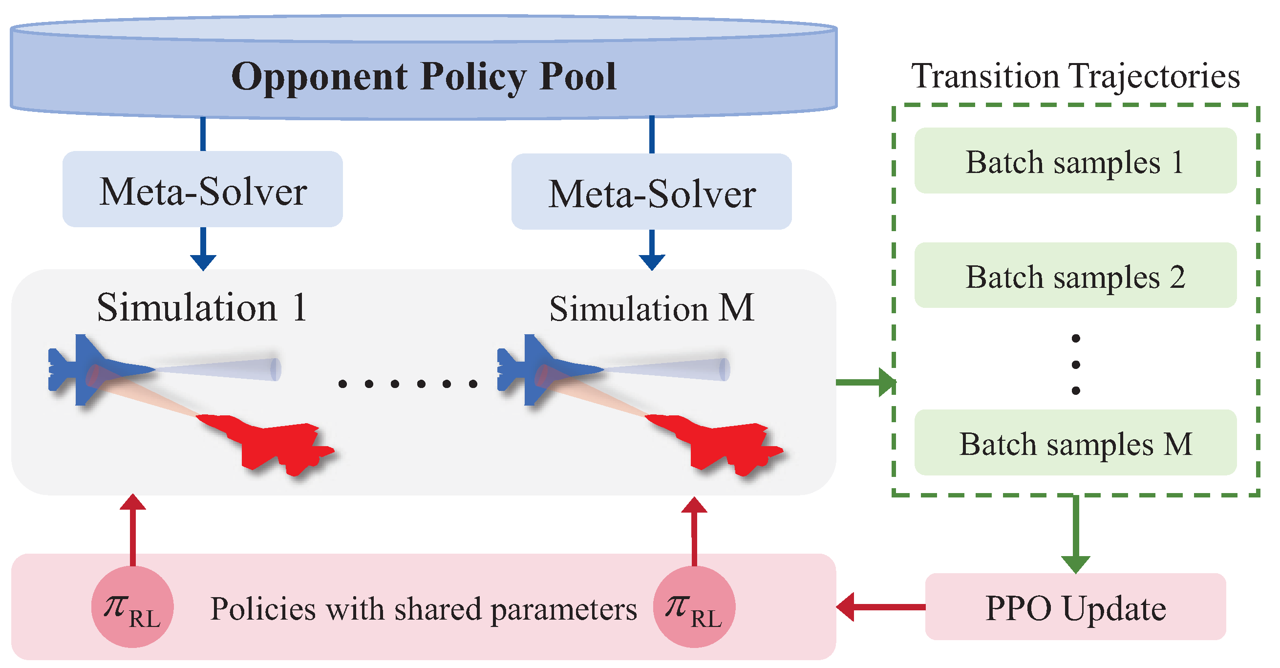
3.4. AOS-PPO with Distributed Training

In the process of training air combat maneuver decision-making through reinforcement learning, the opponent is regarded as a part of the training environment. Since the AOS continuously updates the opponent policy pool through the Gate Function and uses the Meta-Solver to generate a dynamically changing probability distribution for sampling opponents, the environment of RL is dynamically changing. Compared with off-policy RL algorithms, such as the SAC algorithm, on-policy RL algorithms, such as the PPO algorithm, have a better ability to adapt to the dynamic changes of the environment. Therefore, the proximal policy optimization (PPO [34]) algorithm is employed in the proposed automatic-opponent-sampling-based RL framework. Within the improved PPO with AOS framework (AOS-PPO), the actor is the agent’s policy neural network ${\pi }_{\theta }$ with the parameter $\theta$. The critic serves as the objective function for policy optimization. Within this critic, the estimated value function is used to calculate the advantage, which is estimated by the general advantage estimation (GAE) as follows:

$$A_t=\sum _{\tau =t}^{t_f}{\left(\gamma {\lambda }_{\mathrm{A}}\right)}^{t_f-\tau +1}(r_{\tau }+\gamma V_{\phi }\left(s_{\tau +1}\right)-V_{\phi }\left(s_{\tau }\right))$$

(29)

where $V_{\phi }\left(s_{\tau }\right)$ is the output of the critic in PPO, which is a value function neural network with the parameters $\phi$, and ${\lambda }_{\mathrm{A}}$ is the parameter of the GAE. The parameter $\phi$ is updated by an Adam optimizer based on the loss function defined as follows:

$$L_V={\displaystyle \frac{1}{N_{\mathrm{b}}}}\sum _{t=0}^{t_{\mathrm{f}}}{∥V\left(s_t\right)-\sum _{\tau =0}^t{\gamma }^{\tau -1}{r}_{\tau }∥}^2$$

(30)

where $N_{\mathrm{b}}$ is the number of samples in state transition trajectories, and each sample is a tuple $(s_t,a_t,s_{t+1},r_t)$. Within the AOS-PPO algorithm, the clipped objective function $J\left(\theta \right)$ is defined as follows:

$$J\left(\theta \right)=E_{\zeta \sim {\pi }_{{\theta }_s}}\left\{min\left({\displaystyle \frac{{\pi }_{\theta }\left(s_t\right|a_t)}{{\pi }_{{\theta }_s}\left(s_t\right|a_t)}}{A}_t^{{\theta }_s}(s_t,a_t),f_{\mathrm{clip}}\left(x\right)A_t^{{\theta }_s}(s_t,a_t)\right)\right\}$$

(31)

$$f_{\mathrm{clip}}\left(x\right)=\left\{\begin{array}{c}1-\epsilon ,x<1-\epsilon \hfill \\ x,1-\epsilon \le x\le 1+\epsilon \hfill \\ 1+\epsilon ,x>1+\epsilon \hfill \end{array}\right.$$

(32)

where ${\theta }_s$ is the parameter of the old policy, and $\epsilon$ is the clip parameter for controlling the extent of the policy update. For improving the sampling efficiency, the distributed training is incorporated into the AOS framework, as depicted in Figure 7. In this framework, the gradient for the shared policy is computed as follows:

$$\nabla \overline{J}\left(\theta \right)={\displaystyle \frac{1}{M}}\sum _{m=1}^M\nabla J_m\left(\theta \right)$$

(33)

where M is the number of the simulation processes.

Here, the AOS-PPO algorithm is outlined in Algorithm 3. The essential parameters for both the automatic opponent sampling and the PPO algorithm are detailed in

Table 3. The required parameters for automatic opponent sampling.

Parameter	Value
Length of opponent policy pool, $l_{\Omega }$	8
Frequency of storing historical policy, $f_{\Delta }$	50
Frequency of updating $\Omega$, $f_{\Omega }$	50
Initial temperature $T_{\mathrm{b}}$ in SA–Boltzmann	1700 K

and

Table 4. The required parameters of PPO.

Parameter	Value
Discount factor, $\gamma$	$0.97$
Critic iteration times, $I_{\mathrm{C}}$	20
Policy iteration times, $I_{\mathrm{A}}$	20
Sampling batch size in one training epoch, $N_{\mathrm{b}}$	40,000
Number of distributed agents, M	10
Clip parameter, $\epsilon$	$0.2$

, respectively. Additionally, as shown in

Table 5. Actor–critic neural network structure.

Components	Layer Shape	Activation Function
Input layer	(1, 17)	Identity
Hidden layers	(4, 128)	Leaky Relu
Output layer of actor	(1, 4)	Tanh
Output layer of critic	(1, 1)	Identity

, the policy neural network and the value function neural network share the same structure of input layer and hidden layers.

Algorithm 3 AOS-PPO.

1: Initialize actor ${\pi }_{\theta }$, critic $V_{\phi }$, Algorithm 1 and 2   2: for iteration times $k=1,\cdots ,K$ do   3:    for distributed agent = $1,\cdots ,M$ do   4:        Use Algorithm 1 to sample opponent policy   5:        Step dogfight simulation   6:        Store transitions $\left\{s_t,a_t,s_{t+1},r_t\right\}$   7:        Estimated advantages $A_{\theta }(s_t,a_t)$ and store   8:    end for   9:    for policy update times $i=1,\cdots ,I_{\mathrm{A}}$ do 10:        Average policy gradients of distributed agents with Equation (33) 11:        Update policy parameters $\theta$ by Adam [43] 12:    end for 13:    for value function update $I_{\mathrm{C}}$ times do 14:        Calculate the value function loss using all agents’ stored transitions with (30) 15:        Update value function parameters $\phi$ by Adam 16:    end for 17:    Use the Algorithm 2 to update the opponent historical strategy set $\Omega$ 18: end for

4. Results and Discussion

Within this section, in order to evaluate the performance of the AOS-PPO algorithm for dogfighting, we compare it with different algorithms. The maneuvering strategy trained by the AOS-PPO is tested with different opponents, and the computational efficiency is compared too. Moreover, the effectiveness of simulated annealing (SA)-inspired curriculum learning and the Meta-Solver in the AOS framework are studied by ablation experiments. Additionally, the limitations and future possibilities of the proposed AOS-PPO algorithm are discussed.

4.1. Experiment Settings

The training of the dogfight strategy occurs within the aforementioned simulation environment. The simulation rate is 100 Hz, while the rate of maneuvering decision-making is limited to 10 Hz. Furthermore, this simulation environment serves as the testbed for evaluating the performance of the trained dogfight strategy in comparison to other strategies.

In both the training and testing simulations, we establish the initial conditions for the dogfight scenario, as outlined in

Table 6. Initial conditions for simulations.

Parameter	Value
Initial pitch angle for the agent and the opponent, ${\vartheta }_0$	$0°$
Initial roll angle for the agent and the opponent, ${\varphi }_0$	$0°$
Initial yaw angle for the agent and the opponent, ${\psi }_0$	($-180°$, $180°$)
Initial distance between the agent and the opponent, $d_0$	(1000 m, 3000 m)
Initial altitude for the agent and the opponent, $h_0$	(3000 m, 10,000 m)
Initial health point for the agent and the opponent, $\mathrm{HP}$	3 s
Initial antenna train angle for the agent, ${\mu }_0$	($0°$, $180°$)

. Some initial conditions are randomly set within the given scopes. When evaluating the performance of dogfight strategies during training and testing, we consider several key metrics, including the win ratio (WR), Shooting Down Ratio (SDR), and Time of Win (TOW). The Shooting Down Ratio (SDR) indicates the ratio of successfully shooting down opponents to the total number of games played. In cases where victory is not achieved, the TOW is measured as the maximum duration of the dogfight game, which is typically set at 300 s.

4.2. Training and Testing Comparisons

In this work, the proposed AOS-PPO algorithm is compared with different RL algorithms including the PPO algorithm, SAC-lstm algorithm, and improved PPO with the PFSP algorithm. These algorithms are implemented by the authors for training dogfight maneuvering decision-making, sharing the same observations and rewards as the proposed AOS-PPO algorithm. During the training processes of the PFSP-PPO algorithm and the PPO algorithm, the opponents are initialized as the $\kappa$-PPG strategy with $\kappa =0.2$, and then the priority fictitious self-play method and the fictitious self-play method are adopted, respectively. Moreover, the SAC-lstm algorithm employs the $\sigma -\mathrm{Uniform}$ self-play method. As depicted in Figure 8, the AOS-PPO algorithm exhibits a more stable and efficient convergence process. It is noticed that the PPO algorithm and the PFSP-PPO algorithm share the same parameters for PPO with the AOS-PPO algorithm, while the parameters of the SAC-lstm algorithm are rooted in reference [27]. Compared with the PPO and SAC-lstm algorithms, AOS-PPO can explore more effective strategies due to training with easy-to-hard opponents, without overfitting a local optimal strategy due to the improvement of the opponent’s strategy. However, due to the continuous improvement of the opponent’s maneuver decision-making ability during the training process, the AOS-PPO algorithm requires more iterations to converge, and its convergence speed is slightly slower than that of the PPO algorithm and the SAC-lstm algorithm. Moreover, AOS contains multiple components, resulting in a higher computational complexity during training. Therefore, compared with other algorithms, the AOS-PPO algorithm consumes more training time. Different from the PFSP-PPO algorithm, AOS-PPO makes the performance of candidate adversary strategies continuously improve through SA-inspired curriculum learning and the PSW Gate Function, instead of sampling good adversary strategies across the entire set of historical strategies. The diversity of opponents is also enhanced via the SA–Boltzmann Meta-Solver. Hence, compared to the PFSP-PPO algorithm, although the AOS-PPO algorithm does not have a fast convergence speed, it achieves a higher convergence reward.

Furthermore, we compare the strategies obtained from the training of each algorithm with the strategy trained by AOS-PPO. Notice that each test is conducted with 1000 simulations. Moreover, we also conduct adversarial tests between the strategy trained by AOS-PPO and the state–event–condition–action (SECA [21]) hierarchical strategy. The decision-making layer of SECA is an expert system based on jet pilot knowledge from manual [38], and the execution of some actions is achieved through reinforcement learning. For example, reinforcement learning is used to train aiming at the opponent. As shown in

Table 7. Results of testing against different opponents.

Opponents	Agent’s WR	Agent’s SDR	Agent’s TOW	Opponent’s WR	Opponent’s SDR
SAC-lstm	0.545	0.115	289.3	0.341	0.027
PPO	0.722	0.383	266.5	0.187	0.004
PFSP-PPO	0.629	0.276	283.5	0.325	0.034
SECA	0.417	0.361	290.1	0.162	0.03
w/o CL	0.744	0.465	188.39	0.102	0.008
w/o SA–Boltzmann	0.754	0.281	275.3	0.135	0.02

, the AOS-PPO-trained strategy (AOS-PPO agent) has a high win ratio against strategies trained by other RL approaches, further verifying that the AOS-PPO algorithm converges to a better strategy. Due to the large number of close-range air combat cases, pilots have accumulated a great deal of dogfight experience. Therefore, the rule-based SECA strategy also possesses a high capability for dogfight maneuver decision-making. Nevertheless, in contrast to the SECA strategy, by continuously engaging with opponents of a higher skill level, the strategy trained by AOS-PPO learns more complex tactics with more accurate judgments of the situation and a closer connection between maneuvering actions, thus achieving a higher winning rate.

In order to verify the overfitting of the AOS-PPO algorithm and the generalization ability of the trained policy, we deploy experiments for the joint policy correlation (JPC) matrices [33], where different random numbers are used to train five independent policies ${\mathit{\pi }}_{\mathrm{jpc}}=\left\{{\pi }^i,i\in 5\right\}$ with AOS-PPO. The entries of the JPC matrices are defined as follows:

$$\mathrm{WR}\left({\pi }_1^i,{\pi }_2^j\right);{\pi }_1^i,{\pi }_2^j\in {\mathit{\pi }}_{\mathrm{jpc}}$$

(34)

where agent 1 uses the policy ${\pi }_1^i$ and agent 2 uses the policy ${\pi }_2^j$. The win ratio is computed through 1000 simulations. From a JPC matrix, we compute an average proportional loss (APL) [33] in the win ratio as follows:

$$\mathrm{W}{\mathrm{R}}_{-}=\left(\overline{D}-\overline{O}\right)/\overline{D}$$

(35)

where $\overline{D}$ is the value of the diagonals and $\overline{O}$ is the mean value of the off-diagonals. The JPC matrices for AOS-PPO is illustrated in Figure 9, where $\overline{D}=0.362,\overline{O}=0.3298,\mathrm{W}{\mathrm{R}}_{-}=0.089$. It means the policy trained with AOS-PPO can expect to lose 8.9% of its win ratio when playing with another independently trained policy. Additionally, from Table 7, it can be observed that the policy trained using the AOS-PPO algorithm is capable of adapting to different opponents and gaining an advantage in the dogfight game. These demonstrate a good generalization capability when facing new opponents.

4.3. Ablation Study

To further analyze the effectiveness of the AOS framework, we design a set of ablation experiments: (1) w/o CL: the evolution of the opponent policy pool does not include an SA-inspired curriculum learning phase; (2) w/o SA–Boltzmann: the SA–Boltzmann Meta-Solver is replaced with a uniform distribution. It is found that the SA curriculum learning in the phased opponent policy pool and the SA–Boltzmann Meta-Solver improve the performance of the obtained strategy. In the curriculum learning of AOS, the $\kappa$-PPG strategy is adopted to initialize the opponent policy pool. This initialization process endows the initial opponents in the training phase with stable flight capabilities and basic dogfight skills. As the training unfolds, a progressive enhancement mechanism is implemented to incrementally elevate the dogfight proficiency of these opponents. By virtue of this approach, AOS-PPO is enabled to explore effective maneuver strategies from the beginning of the training. Conversely, the strategies that the w/o CL algorithm commences to learn at the training onset are either non-functional or of a considerably low skill level. Moreover, the SA–Boltzmann Meta-Solver empowers the AOS algorithm to take into account both the diversity of opponents and their dogfight capabilities during training, facilitating the AOS-PPO algorithm learning superior maneuvering strategies. Therefore, as shown in Table 7 and

Table 8. Training results as WR, SDR, and TOW.

Methods	WR	SDR	TOW
AOS-PPO	0.818	0.751	107.81
w/o CL	0.754	0.677	133.16
w/o SA–Boltzmann	0.758	0.683	131.1

, the proposed AOS-PPO algorithm achieves higher win ratios compared to the w/o CL algorithm and the w/o SA–Boltzmann algorithm, and the AOS-PPO agent can defeat the w/o CL and w/o SA–Boltzmann algorithms with high win ratios.

4.4. Computational Efficiency

In order to analyze the computational efficiency of the neural network trained by the AOS-PPO algorithm, we deploy it on an embedded computer (NVIDIA Jeston TX2 (NVIDIA, Santa Clara, CA, USA)) for real-time computation and compare it with different algorithms. As shown in

Table 9. Comparison of computational efficiency between algorithms.

Algorithm	Computation Time per Decision
AOS-PPO	0.028 s
PFSP-PPO	0.029 s
SAC-lstm	0.041 s
SECA	0.012 s

, the opponents of the algorithms are the strategies trained via the PPO algorithm. The strategies from the AOS-PPO algorithm and the PFSP-PPO algorithm have almost the same computational speed. The SECA agent is composed of a rule-based strategy and neural networks with very few parameters, and it is computationally small and runs the fastest. Due to the simpler structure and fewer parameters of the MLP neural network of the AOS-PPO algorithm, its computational speed is faster compared to the long short-term memory (lstm) neural network trained by the SAC-lstm algorithm. Since the decision frequency required by the AOS-PPO agent is 10 Hz (obtaining real-time situational inputs and making decisions every 0.1 s) and the computational speed of the trained strategies is 0.028 s, we believe that the AOS-PPO trained strategies can be used to make real-time decisions in real scenarios.

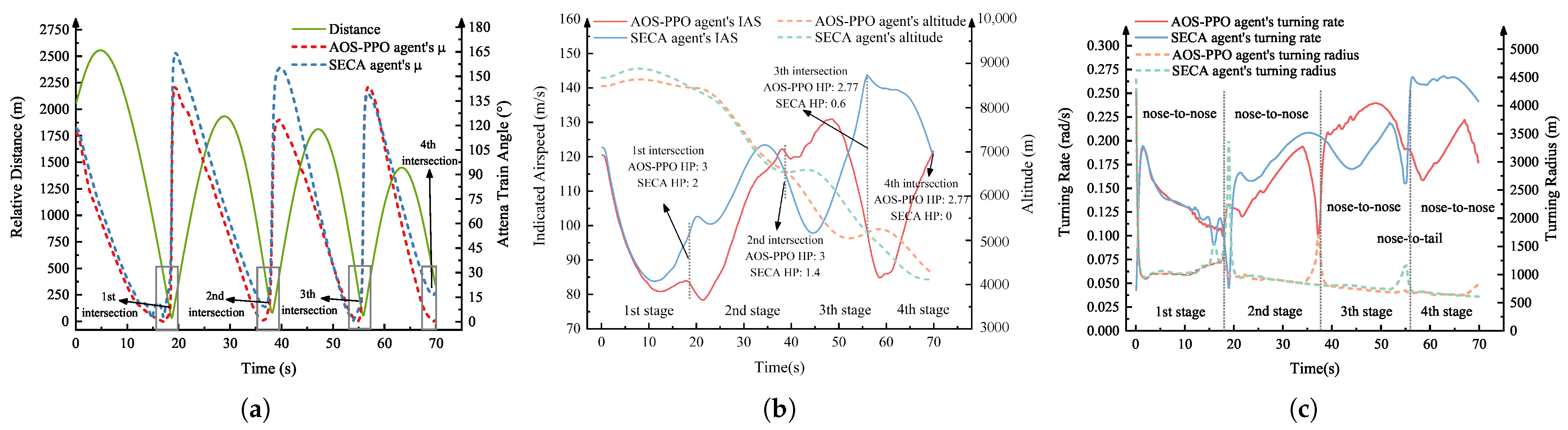
4.5. Simulation Analysis

To uncover the hidden tactics within the policy trained by the AOS-PPO algorithm and understand the reasons behind its victories, we observe and analyze all the test simulations. We discover a common dogfight process that the AOS-PPO agent has mastered: a tactic called ‘vertical maneuvering’, which allows it to quickly align its WEZ with the opponent. However, as shown in Figure 10, during the dogfight process, both sides continuously descend in altitude, eventually engaging in a dangerous low-altitude dogfight. As depicted in Figure 11, in this low-altitude engagement, the AOS-PPO agent is able to maintain a safe altitude and speed while continuously maneuvering towards the opponent. It delivers a decisive blow when the opponent makes a mistake (such as poor altitude control leading to a near-ground collision and a forced pull up).

Furthermore, during many simulations, the AOS-PPO agent presents some highly effective vertical maneuvering tactics. For example, as depicted in Figure 12, this dogfight process of the AOS-PPO agent using vertical maneuvering tactics can be divided into four stages with four instances of intersection between the two sides. We will now analyze the dogfight process in these four stages.

First stage. As shown in Figure 13, initially, both the red (AOS-PPO) and blue (SECA) sides have the same altitude, speed, and ATA. The AOS-PPO agent and the SECA agent each turn towards the other side, entering the nose-to-nose turn [38]. Before reaching the first intersection, the AOS-PPO agent exhibits more stable control, aligns its Weapon Engagement Zone (WEZ) with the opponent, and decelerates to secure a longer shooting duration.

Second stage. As depicted in Figure 12, after the first intersection, both sides enter a nose-to-nose turn again. The AOS-PPO agent has a lower speed and a smaller turning radius, enabling it to aim at the opponent more quickly. Additionally, due to vertical maneuvering and rapid descent, the AOS-PPO agent maintains a certain speed.

Third stage. During the second intersection, the AOS-PPO agent continues to opt for a quick Spilt-S maneuver for vertical engagement. In contrast, the opponent initially performs a horizontal turn, which demands an exceptionally fast turn rate to align with the AOS-PPO agent—a challenging feat for the opponent. Consequently, when the opponent eventually transitions into vertical maneuvering, it has already lost the advantages of low speed and a small turning radius inherent in the nose-to-nose turn.

Fourth stage. As shown in Figure 12 and Figure 13, prior to the third intersection, the AOS-PPO agent is in a climbing state while the opponent is in a diving state. If both sides maintain their original attitudes and load factors after the intersection, they would enter a nose-to-tail turn, which would be highly disadvantageous for the low-speed AOS-PPO agent. Therefore, after the intersection, the AOS-PPO agent quickly transitions into a downward nose-to-nose turn through a barrel roll maneuver. This allows the AOS-PPO agent to gain the advantage of low speed and a small turning radius. As a result, the AOS-PPO agent manages to shoot down the opponent before the fourth intersection.

4.6. Limitations and Future Works

On the one hand, the realistic scenario is more complex than the simulation. Firstly, the agent’s perception of the opponent may be discontinuous or noisy, and the PPO algorithm and neural network in the method proposed in this paper may find it hard to adapt to such complex observation constraints. Secondly, as depicted in Figure 12, during a dogfight, both sides will continuously decrease their altitude to obtain the sufficient indicated airspeed for turning and aiming at the opponent. However, in the realistic scenario, there may be complex terrain constraints such as mountains and plateaus. The proposed AOS-PPO algorithm and the trained strategies may struggle to adapt to such situations. On the other hand, this study has examined the air combat maneuvering decision-making between aircraft of the same type. However, in reality, the opponents may possess different maneuvering capabilities. Within air combat maneuvering decision-making, differences in maneuvering capabilities will lead to significant changes in tactics, and the strategies obtained through the training in this study may have difficulty adapting to such changes.

Our future works will extend to autonomous air combat decision-making with complex terrain constraints and perception uncertainties. Moreover, based on the proposed AOS method, we will further consider the diversity of the opponents’ maneuvering capabilities to enrich the strategies and tactics obtained through training. In addition, the proposed AOS-PPO algorithm will also be extended to the cooperative air combat decision-making scenario.

5. Conclusions

In this study, an automatic opponent sampling (AOS) framework is proposed to improve learning efficiency and the strategies’ adaptability to various opponents. Our training results underscore the effectiveness of the AOS framework, which significantly improves the performance of the PPO algorithm for dogfights. Furthermore, our test results demonstrate that policies trained via the AOS-PPO algorithm exhibit impressive dogfight performance and generalization capabilities. These policies can adeptly, consistently, and swiftly maneuver fighter aircraft into advantageous positions through vertical maneuvering tactics. This research not only offers a valuable algorithm for rapidly developing generalized and skilled air combat strategies using Deep Reinforcement Learning but also provides a valuable framework for the design of self-play-based RL algorithms for other aerial game scenarios. Our future work will focus on improving the proposed AOS-PPO algorithm for more realistic scenarios and extending it to collaborative aerial confrontation decision-making.

References

1. Duan, H.; Lei, Y.; Xia, J.; Deng, Y.; Shi, Y. Autonomous Maneuver Decision for Unmanned Aerial Vehicle via Improved Pigeon-Inspired Optimization. IEEE Trans. Aerosp. Electron. Syst. 2023, 59, 3156–3170. [Google Scholar]
2. Jing, X.; Cong, F.; Huang, J.; Tian, C.; Su, Z. Autonomous Maneuvering Decision-Making Algorithm for Unmanned Aerial Vehicles Based on Node Clustering and Deep Deterministic Policy Gradient. Aerospace 2024, 11, 1055. [Google Scholar] [CrossRef]
3. Fan, Z.; Xu, Y.; Kang, Y.; Luo, D. Air Combat Maneuver Decision Method Based on A3C Deep Reinforcement Learning. Machines 2022, 10, 1033. [Google Scholar] [CrossRef]
4. Zhu, J.; Kuang, M.; Zhou, W.; Shi, H.; Zhu, J.; Han, X. Mastering air combat game with deep reinforcement learning. Def. Technol. 2024, 34, 295–312. [Google Scholar] [CrossRef]
5. Sun, Z.; Piao, H.; Yang, Z.; Zhao, Y.; Zhan, G.; Zhou, D.; Meng, G.; Chen, H.; Chen, X.; Qu, B. Multi-agent hierarchical policy gradient for Air Combat Tactics emergence via self-play. Eng. Appl. Artif. Intell. 2021, 98, 104112. [Google Scholar] [CrossRef]
6. Choi, J.; Seo, M.; Shin, H.S.; Oh, H. Adversarial Swarm Defence Using Multiple Fixed-Wing Unmanned Aerial Vehicles. IEEE Trans. Aerosp. Electron. Syst. 2022, 58, 5204–5219. [Google Scholar]
7. Ren, Z.; Zhang, D.; Tang, S.; Xiong, W.; Yang, S.H. Cooperative maneuver decision making for multi-UAV air combat based on incomplete information dynamic game. Def. Technol. 2023, 27, 308–317. [Google Scholar]
8. Huang, L.; Zhu, Q. A Dynamic Game Framework for Rational and Persistent Robot Deception With an Application to Deceptive Pursuit-Evasion. IEEE Trans. Autom. Sci. Eng. 2022, 19, 2918–2932. [Google Scholar] [CrossRef]
9. Wang, L.; Wang, J.; Liu, H.; Yue, T. Decision-Making Strategies for Close-Range Air Combat Based on Reinforcement Learning with Variable-Scale Actions. Aerospace 2023, 10, 401. [Google Scholar] [CrossRef]
10. Li, Y.F.; Shi, J.P.; Jiang, W.; Zhang, W.G.; Lyu, Y.X. Autonomous maneuver decision-making for a UCAV in short-range aerial combat based on an MS-DDQN algorithm. Def. Technol. 2022, 18, 1697–1714. [Google Scholar]
11. Singh, R.; Bhushan, B. Evolving Intelligent System for Trajectory Tracking of Unmanned Aerial Vehicles. IEEE Trans. Autom. Sci. Eng. 2022, 19, 1971–1984. [Google Scholar] [CrossRef]
12. Durán-Delfín, J.E.; García-Beltrán, C.; Guerrero-Sánchez, M.; Valencia-Palomo, G.; Hernández-González, O. Modeling and Passivity-Based Control for a convertible fixed-wing VTOL. Appl. Math. Comput. 2024, 461, 128298. [Google Scholar] [CrossRef]
13. Zhang, J.D.; Yu, Y.F.; Zheng, L.H.; Yang, Q.M.; Shi, G.Q.; Wu, Y. Situational continuity-based air combat autonomous maneuvering decision-making. Def. Technol. 2023, 29, 66–79. [Google Scholar] [CrossRef]
14. Dong, Y.; Ai, J.; Liu, J. Guidance and control for own aircraft in the autonomous air combat: A historical review and future prospects. J. Aerosp. Eng. 2019, 233, 5943–5991. [Google Scholar] [CrossRef]
15. Horie, K.; Conway, B. Optimal Fighter Pursuit-Evasion Maneuvers Found Via Two-Sided Optimization. J. Guid. Control. Dyn. 2006, 29, 105–112. [Google Scholar] [CrossRef]
16. Taylor, L. Application of the epsilon technique to a realistic optimal pursuit-evasion problem. J. Optim. Theory Appl. 1975, 15, 685–702. [Google Scholar] [CrossRef]
17. Anderson, G. A real-time closed-loop solution method for a class of nonlinear differential games. IEEE Trans. Autom. Control. 1972, 17, 576–577. [Google Scholar] [CrossRef]
18. Jarmark, B.; Merz, A.; Breakwell, J. The variable-speed tail-chase aerial combat problem. J. Guid. Control. Dyn. 1981, 4, 323–328. [Google Scholar]
19. Ramírez, L.; Żbikowski, R. Effectiveness of Autonomous Decision Making for Unmanned Combat Aerial Vehicles in Dogfight Engagements. J. Guid. Control. Dyn. 2018, 41, 1021–1024. [Google Scholar] [CrossRef]
20. Wu, A.; Yang, R.; Liang, X.; Zhang, J.; Qi, D.; Wang, N. Visual Range Maneuver Decision of Unmanned Combat Aerial Vehicle Based on Fuzzy Reasoning. Int. J. Fuzzy Syst. 2022, 24, 519–536. [Google Scholar] [CrossRef]
21. Hou, Y.; Liang, X.; Zhang, J.; Lv, M.; Yang, A. Hierarchical Decision-Making Framework for Multiple UCAVs Autonomous Confrontation. IEEE Trans. Veh. Technol. 2023, 72, 13953–13968. [Google Scholar]
22. Li, K.; Liu, H.; Jiu, B.; Pu, W.; Peng, X.; Yan, J. Knowledge-Aided Model-Based Reinforcement Learning for Anti-Jamming Strategy Learning. IEEE Trans. Aerosp. Electron. Syst. 2024, 60, 2976–2994. [Google Scholar]
23. Berner, C.; Brockman, G.; Chan, B.; Cheung, V.; Dębiak, P.; Dennison, C.; Farhi, D.; Fischer, Q.; Hashme, S.; Hesse, C.; et al. Dota 2 with Large Scale Deep Reinforcement Learning. arXiv 2019, arXiv:1912.06680. [Google Scholar]
24. Vinyals, O.; Babuschkin, I.; Czarnecki, W.M.; Mathieu, M.; Dudzik, A.; Chung, J. Grandmaster level in StarCraft II using multi-agent reinforcement learning. Nature 2019, 575, 350–354. [Google Scholar]
25. Peng, C.; Zhang, H.; He, Y.; Ma, J. State-Following-Kernel-Based Online Reinforcement Learning Guidance Law Against Maneuvering Target. IEEE Trans. Aerosp. Electron. Syst. 2022, 58, 5784–5797. [Google Scholar]
26. Pope, A.P.; Ide, J.S.; Mićović, D.; Diaz, H.; Twedt, J.C.; Alcedo, K.; Walker, T.T.; Rosenbluth, D.; Ritholtz, L.; Javorsek, D. Hierarchical Reinforcement Learning for Air Combat At DARPA’s AlphaDogfight Trials. IEEE Trans. Artif. Intell. 2022, 4, 1371–1385. [Google Scholar]
27. Bae, J.H.; Jung, H.; Kim, S.; Kim, S.; Kim, Y.D. Deep Reinforcement Learning-Based Air-to-Air Combat Maneuver Generation in a Realistic Environment. IEEE Access 2023, 11, 26427–26440. [Google Scholar] [CrossRef]
28. Zhang, H.; Huang, C. Maneuver Decision-Making of Deep Learning for UCAV Thorough Azimuth Angles. IEEE Access 2020, 8, 12976–12987. [Google Scholar]
29. Yang, Q.; Zhang, J.; Shi, G.; Hu, J.; Wu, Y. Maneuver Decision of UAV in Short-Range Air Combat Based on Deep Reinforcement Learning. IEEE Access 2020, 8, 363–378. [Google Scholar]
30. Bansal, T.; Pachocki, J.; Sidor, S.; Sutskever, I.; Mordatch, I. Emergent Complexity via Multi-Agent Competition. arXiv 2018, arXiv:1710.03748. [Google Scholar]
31. Heinrich, J.; Lanctot, M.; Silver, D. Fictitious Self-Play in Extensive-Form Games. In Proceedings of the 32nd International Conference on Machine Learning, Lille, France, 7–9 July 2015; Volume 37, pp. 805–813. [Google Scholar]
32. Heinrich, J.; Silver, D. Deep Reinforcement Learning from Self-Play in Imperfect-Information Games. arXiv 2016, arXiv:1603.01121. [Google Scholar]
33. Lanctot, M.; Zambaldi, V.; Gruslys, A.; Lazaridou, A.; Tuyls, K.; Pérolat, J.; Silver, D.; Graepel, T. A Unified Game-Theoretic Approach to Multiagent Reinforcement Learning. In Proceedings of the Advances in Neural Information Processing Systems, Long Beach, CA, USA, 4–9 December 2017; Guyon, E.I., Ed.; Curran Associates, Inc.: Red Hook, NY, USA, 2017; Volume 30. [Google Scholar]
34. Schulman, J.; Wolski, F.; Dhariwal, P.; Radford, A.; Klimov, O. Proximal Policy Optimization Algorithms. arXiv 2017, arXiv:1707.06347. [Google Scholar]
35. Haarnoja, T.; Zhou, A.; Abbeel, P.; Levine, S. Soft Actor-Critic: Off-Policy Maximum Entropy Deep Reinforcement Learning with a Stochastic Actor. In Proceedings of the International Conference on Machine Learning, Pmlr, Stockholm, Sweden, 10–15 July 2018; pp. 1861–1870. [Google Scholar]
36. Stevens, B.; Lewis, F.; Johnson, E. Aircraft Control and Simulation: Dynamics, Controls Design, and Autonomous Systems, 3rd ed.; WILEY: Hoboken, NJ, USA, 2015. [Google Scholar]
37. Mataric, M. Reward Functions for Accelerated Learning. In Machine Learning Proceedings 1994; Elsevier: Amsterdam, The Netherlands, 1994; pp. 181–189. [Google Scholar]
38. Shaw, R. “Fighter Combat,” Tactics and Maneuvering; Naval Institute Press: Annapolis, MD, USA, 1986. [Google Scholar]
39. Ulrich, B. Brown’s original fictitious play. J. Econ. Theory 2007, 135, 572–578. [Google Scholar]
40. Hernandez, D.; Denamganai, K.; Devlin, S.; Samothrakis, S.; Walker, J.A. A Comparison of Self-Play Algorithms Under a Generalized Framework. IEEE Trans. Games 2022, 14, 221–231. [Google Scholar] [CrossRef]
41. Bengio, Y.; Louradour, J.; Collobert, R.; Weston, J. Curriculum learning. In Proceedings of the 26th Annual International Conference on Machine Learning, Montreal, QC, Canada, 14–18 June 2009; pp. 41–48. [Google Scholar]
42. Baker, B.; Kanitscheider, I.; Markov, T.; Wu, Y.; Powell, G.; McGrew, B.; Mordatch, I. Emergent Tool Use From Multi-Agent Autocurricula. In Proceedings of the International Conference on Learning Representations, Addis Ababa, Ethiopia, 30 April 2020. [Google Scholar]
43. Kingma, D.P.; Ba, J. Adam: A Method for Stochastic Optimization. arXiv 2014, arXiv:1412.6980. [Google Scholar]
Figure 1. The simulation environment is employed with a simulated flight controller and 6-DOF aircraft dynamic model.
Aerospace 12 00265 g001
Figure 2. Three-dimensional geometric parameters of the dogfight and the scope of the Weapons Engagement Zone (WEZ).
Aerospace 12 00265 g002
Figure 3. The framework of the PSRO for symmetric games like dogfights.
Aerospace 12 00265 g003
Figure 4. AOS framework with a phased opponent policy pool, an SA–Boltzmann Meta-Solver, and a priority sliding window (PSW) Gate Function.
Aerospace 12 00265 g004
Figure 5. Opponent pursues the LOS or in a random direction using the κ -PPG policy in the SA-inspired CL phase.
Aerospace 12 00265 g005
Figure 6. The process of updating the Ω by the PSW-GF.
Aerospace 12 00265 g006
Figure 7. Distributed training framework for AOS-PPO.
Aerospace 12 00265 g007
Figure 8. The average normalized episode rewards of the training experiments. The training experiments are conducted using a Lenovo computer which are sourced from Beijing, China (1 AMD Ryzen Threadripper PRO 3975WX CPU, 1 NVIDIA GeForce RTX 3090 GPU, 4 Kingston 32GB DDR4 memory modules). The training time of each algorithm is as follows: AOS-PPO, 49.6 h; SAC-lstm, 35.12 h; PPO, 33.27 h; PFSP-PPO, 45.6 h.
Aerospace 12 00265 g008
Figure 9. The JPC matrices for AOS-PPO in the dogfight game. The elements are the average win rates of agent 1 against agent 2, and the confidence intervals (0.95) are shown in parentheses.
Aerospace 12 00265 g009
Figure 10. Trajectory and progress (time: (HP, μ , v ias )) of vertical maneuvering and ‘low-altitude’ engagement: (a) vertical maneuvering, (b) ‘low-altitude’ engagement.
Aerospace 12 00265 g010
Figure 11. A common dogfight process example of the ‘vertical maneuvering’ tactic and ‘low-altitude’ engagement: (a) comparison of altitude, (b) comparison of distance and ATA.
Aerospace 12 00265 g011
Figure 12. Trajectory and progress (time: (HP, μ )) of highly effective vertical maneuvering.
Aerospace 12 00265 g012
Figure 13. The dogfight process of the AOS-PPO agent and its opponent with highly effective vertical maneuvering: (a) comparison of distance and ATA, (b) comparison of IAS and altitude, (c) comparison of turning rate and radius.
Aerospace 12 00265 g013