Abstract
In recent years, global navigation satellite system (GNSS)-based navigation in high earth orbits (HEOs) has become a field of research interest since it can increase the spacecraft’s autonomy, thereby reducing the operating costs. However, the GNSS availability and the GNSS-based navigation performance for a spacecraft orbiting above the GNSS constellation are strongly constrained by the signals’ power levels at the receiver position and the sensitivity. The simulated level of signal power at the receiver’s position may considerably increase or decrease when assuming different gain/attenuation values of the transmitter antenna for a certain azimuth and elevation. Assuming a slightly different antenna pattern therefore may significantly change the simulated signal’s availability results and accordingly the simulated navigation accuracy, leading to an inexact identification of the requirements for the GNSS receiver. This problem particularly concerns the case of orbital trajectories above the GNSS constellation, where most of the signals received are radiated from the secondary lobe of the transmitters’ antennas, for which typically very little information is known. At the time of this study, it was possible to model quite accurately the global positioning system (GPS) L1 antenna patterns for the IIR and IIR-M Blocks because of the precise information available. No accurate information was available for the GPS L1 antenna patterns of the IIF Block. Even less accurate information was available on the GPS L5 antenna patterns. In this context, this paper aims at investigating the effect of different antenna pattern assumptions on the simulated signal availability and on the consequent simulated navigation performance of a spaceborne receiver orbiting in a very highly elliptical orbit from the Earth to the Moon. Initially the impact of averaging the transmitter’s antenna gain over the azimuth, a typical assumption in many studies, is analyzed. Afterwards, we also consider three different L5 antenna patterns assumed in the literature (the precise L5 patterns are unfortunately not yet fully available). For each of the considered antenna pattern assumptions, we simulate received signal power level, availability, geometric dilution of precision (GDOP), and navigation accuracy in order to evaluate their different effects. After identifying the most conservative assumptions for the transmitters’ antenna patterns, for each elevation of the receiver antenna, we also compute the number of available GNSS observations and analyze their distribution. Moreover, possible aiding of the acquisition process using the prediction of the elevation at which the signal is transmitted, as well as the elevation at which the signal is received, are discussed. Finally, the impact on the GDOP of using only signals transmitted from certain angle intervals of the transmitter antenna pattern and the importance of selecting the transmitters that provide the best GDOP (in the case of a receiver with a limited number of channels) are considered and discussed.
1. Introduction
Global navigation satellite system (GNSS) in space applications started to be investigated in the mid to late 1970s, while in 1982 the first spacecraft flew with an onboard spaceborne receiver [1]. Since then, the use of GNSS at low earth orbit (LEO) has been successfully adopted, favored by the strong signal powers and the good relative geometry that a receiver at these altitudes experiences. Moreover, the great benefits of GNSS-based navigation over conventional ground-based methods, such as increased spacecraft’s autonomy and reduced operational costs, as well as the will to improve the achieved accuracy, motivated the investigation of global positioning system (GPS) at higher altitudes, leading to the first recordings beyond LEO in 1997. The eagerness to exploit GNSS signals at higher orbits has increased in recent years, keeping in mind new innovations such as improved weather prediction, exploration moon missions and beyond, formation flying, etc.
Although space users showed great enthusiasm for GNSS-based navigation, they had to face important difficulties compared to earth users. Indeed, primarily intended for earth navigation, initial GPS system specifications (such as minimum received power level and availability) covered only earth users or up to 14° half angle of the transmitters’ antenna [1]. Due to the great utility for space users above 14° and the significant changes between the different blocks, space users wanted formal specifications to be included. Efforts to include space service volume (SSV) did not start until the 1990s and it was in February 2000 when space requirements were officially included. However, this was not enough, and further improvements were needed. GPS III included new space requirements: (1) SSV was further subdivided in two regions, medium earth orbit space service volume (MEO SSV) (3000–8000 km) and geostationary earth orbit/high earth orbit space service volume (GEO/HEO SSV) (8000–36,000 km) and (2) specified worst case signal strength and availability. Even though it is clear that processing signals from the side lobes can significantly improve the availability (and the receiver/transmitters geometry) in GEO/HEO, so far, for many GNSS signals and GNSS satellites blocks, detailed specifications of the transmitters’ side lobes have not been yet explicitly stated. As stated in [2], “Protection of GPS Side Lobes through Specification is critically important to ‘Do No Harm’ to current and future users of SSV”. Under these circumstances, a GPS receiver in GEO/HEO should be able to process signals transmitted from the side lobes of the GPS antenna patterns. The lower power levels that these signals have, compared to the ones transmitted from the main lobe, affect the range accuracy with higher receiver noise. Moreover, if the receiver’s sensitivity is not high enough, the availability of GNSS signals can be drastically lower, with a consequent worsening of the geometric dilution of position (GDOP), or in the worst case preventing the computation of the navigation solution, for which at least four observations are needed.
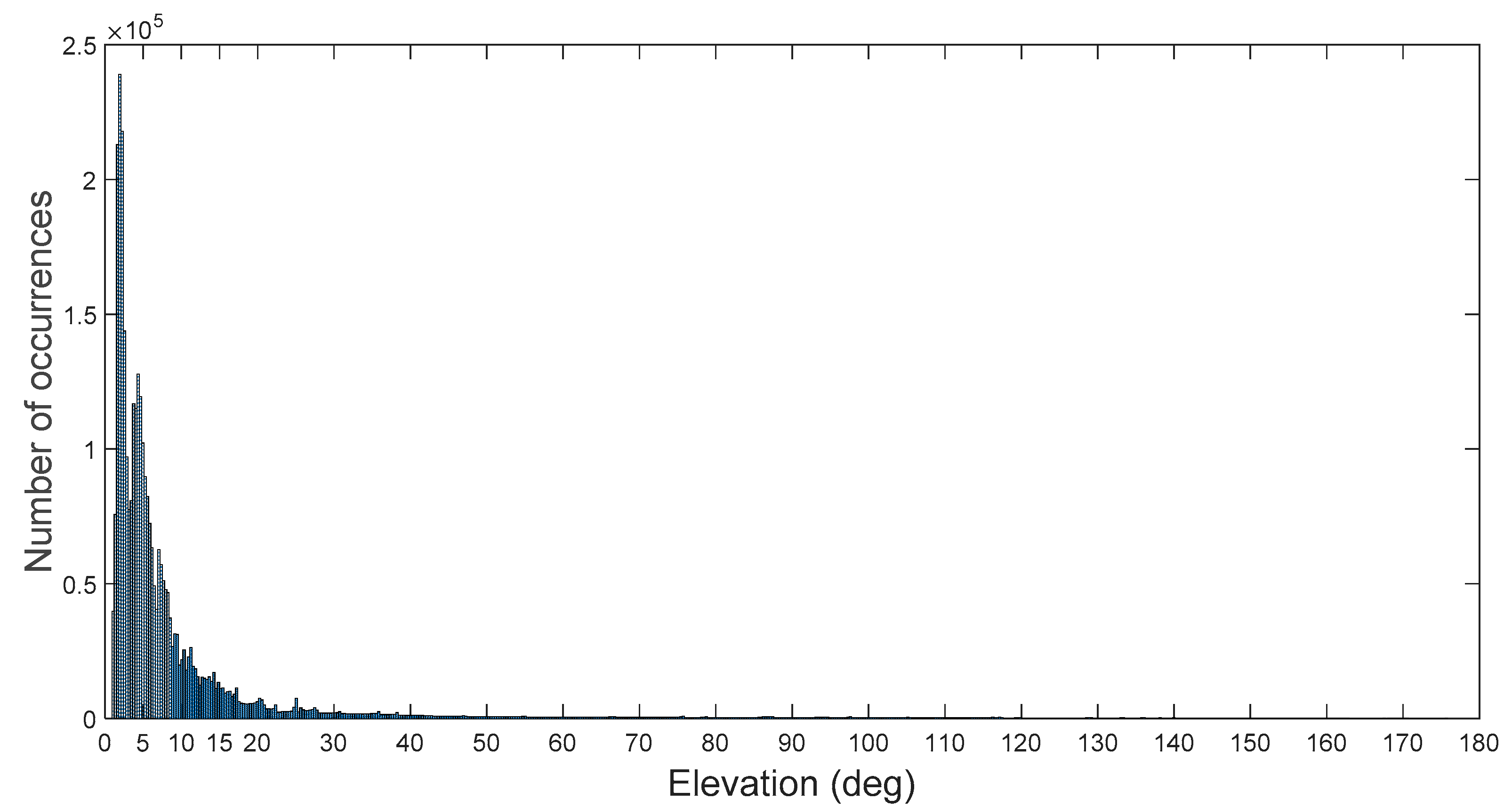
In this context, in order to correctly simulate the GNSS-based navigation performance of a spaceborne receiver, the assumptions on the GNSS antenna patterns are very important and delicate, especially on the side lobes. The main lobe is well known and no assumptions are needed. Figure 1 and Figure 2 show, respectively, the angle from the antenna boresight at which the signals are transmitted by the GPS satellites (for each pseudo random noise (PRN)) and the number of signals that have been transmitted from the main lobe or the side lobes, for a direct moon transfer orbit (MTO), presented in Section 2. As can be observed, in the case of space users operating in all SSV and up to the Moon, most of the signals would be acquired and tracked from the side lobes. Evidently, correctly modeling the side lobes of the transmitters’ antennas is very important as it would directly affect the navigation performance at the high altitudes obtained in simulation.
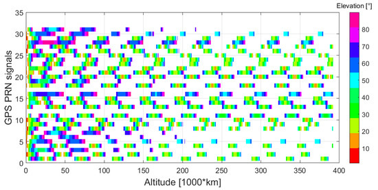
Figure 1.
Elevation angle of the global positioning system (GPS) antenna pattern from which the signals are received, for the assumed moon transfer orbit (MTO) in Section 2.1.
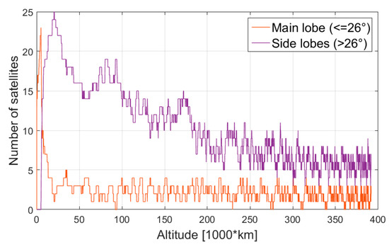
Figure 2.
Number of GPS satellites received from main and side lobes of the transmitters’ antenna pattern, for the assumed MTO in Section 2.1.
In the case of GPS L1 and L2, antenna gain data and relative phase data has been released for Blocks IIR and IIR-M [3]. On the other side, Boeing, which is responsible for building GPS Block IIF satellites, has not released any similar document yet. Even more obscure is the information regarding GPS L5 antenna directivity data. Existing information used by researchers is usually an approximation of the expected patterns using the information in [4]. No definite data have been released so far, causing possible inaccuracies in the results of the published researches. In [5], for instance, only an example of L5 pattern for only one PRN (PRN 5, from block IIR-M) is reported, and without detailing how this pattern was approximated from the available data.
In our previous research [6], we investigated the feasibility of using GNSS as navigation system to reach the Moon; in [7] we described the implementation of an orbital filter in order to improve the navigation accuracy; in [8] we detailed how such a filter can be used for aiding purposes; in [9] we demonstrated the GNSS accuracy at GEO altitude achieved with the developed orbital filter considering that the receiver is able to process different signal combinations. However, the lack of information about the transmitters’ antenna patterns has always limited the level of accuracy. Considering the importance of the antenna pattern assumptions, in this research we aim to evaluate the effects of different antenna pattern assumptions when simulating the performance of a GNSS-based navigation system for space missions, in order to identify the most conservative assumptions to be used in our future simulations and tests. Elements like experienced signal levels, availability, GDOP and ranging error were computed for different antenna patterns assumptions. Moreover, the impact of different antenna pattern assumptions on the navigation solutions obtained using the single-point least squares technique and an orbital filter was analyzed. Initially, we evaluated the effect of averaging the gain pattern in azimuth for the GPS L1 signals and then we explored the impact of assuming different GPS L5 patterns available from the literature. Furthermore, information on the elevation angles of the transmitter and receiver antenna patterns of the available GNSS signals is also considered and analyzed.
These evaluations were carried out considering the characteristics of the “SANAG” (spaceborne autonomous navigation based on GNSS) receiver, a proof-of-concept GPS receiver under development in our laboratory, specifically for lunar missions. The considered MTO is an interesting trajectory case, as it includes the signals’ characteristics of the SSV and beyond, up to the Moon.
Following a description of the models and assumptions (in Section 2), in the first part of the paper (in Section 3 and Section 4), we analyze the effect of assuming different transmitter antenna patterns on the signal power level at the receiver’s position, on the availability, on the GDOP, and finally on the navigation accuracy. The analysis was performed for the signals that the SANAG receiver can process and then for GPS L1 C/A (in Section 3) and for GPS L5 (Section 4), for which we considered different antenna patterns information publically available. Once we have identified the most conservative antenna patterns both for L1 and L5 (in Section 5), we focus on the elevation at which the signals are received during the full MTO; such a study can provide useful information for the design of the receiver antenna, specifically for the mission considered. Furthermore (in Section 6), we investigate the relationship between the signal’s availability at the receiver’s position and the angle from the transmitter antenna’s boresight at which the same signal was transmitted. As specified in this manuscript (in the beginning of Section 6), this relation is of interest since the prediction of the elevation at which the signal is transmitted, as well as the elevation at which the signal is received, combined with the knowledge of the transmitter and receiver antenna patterns, can be used to aid the acquisition process and better attribute the available tracking channels. Similarly (in Section 7), we also analyze the relationship between the angle at which the signals are transmitted from the GPS satellites and their relative geometry with respect to the receiver, which can also be exploited to aid in the signal acquisition process. Finally, Section 8 gives a summary of the conclusions obtained during this work.
2. Models and Assumptions
For our simulations, the highly accurate multi-GNSS simulator “Spirent GSS8000” was used to simulate realistic GPS signals for different antenna patterns [10]. Basically, we defined the trajectory, the antenna patterns, the transmitters’ ephemeris, the signal level characteristics of all simulated carrier frequencies at the radio frequency (RF) output, and the Spirent simulator provided simulated signals power levels at the receiver position. In our tests, we defined the GPS constellation of 29 satellites according to the almanac of 1 July 2005. The other assumptions are presented in the following paragraphs of this section.
2.1. Receiver’s Dynamics and Kinematics
For this work, an accurate MTO trajectory of the receiver was generated using the Astrogator Tool of system tool kit (STK) [11], and after provided as reference trajectory in our Spirent simulator, as user motion text (UMT) (user motion) file.
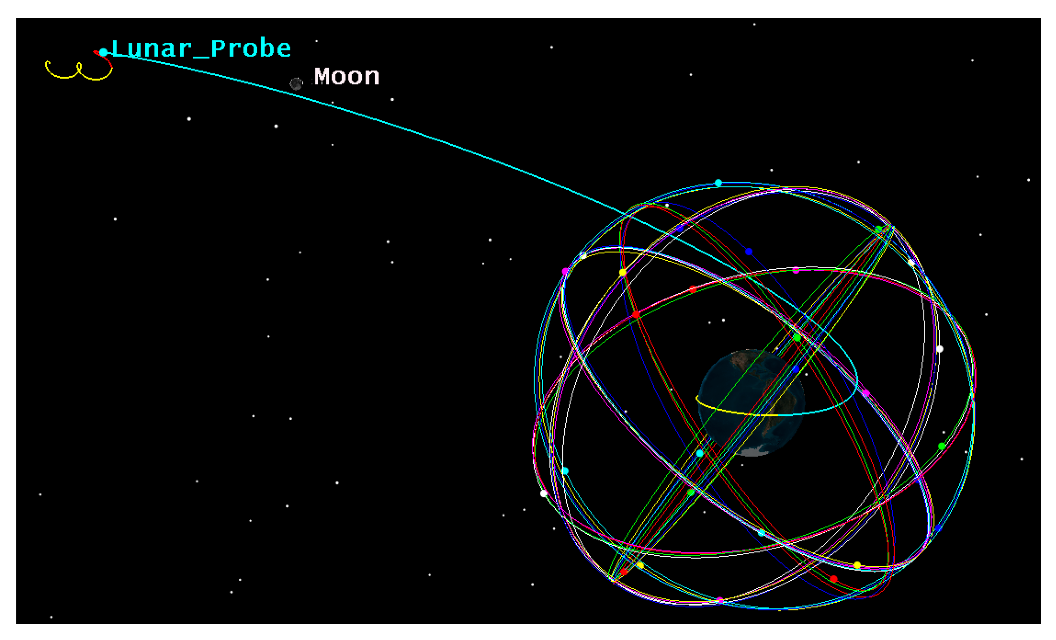
The considered MTO is illustrated in Figure 3, where is identified by the yellow curve in LEO and the blue curve in HEO with perigee at the Moon altitude. In this trajectory, a GNSS receiver experiences all signal characteristics that it would experience orbiting at different altitudes in space (from LEO to the Moon).
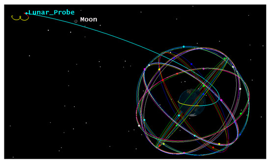
Figure 3.
Assumed MTO for the receiver.
The initial time of investigation is 18:10:00 on 1 July 2005, while the launch of the vehicle was performed earlier. The investigated part of this study is propagated until 05:11:12 on 6 July 2005, which corresponds to the end of the blue curve (Moon altitude); it experiences an impulsive acceleration of 3.14217 km/s2 in the x-axis, at time 18:41:37:154 on 1 July 2005, to change the orbit from LEO to HEO with a perigee at Moon altitude. The initial earth centered inertial (ECI) position and velocity coordinates of the investigated trajectory are (−6188.944987; 1742.455236; 1155.838277) km and (2.484942; −6.510775; 3.563661) km/s, respectively.
2.2. Assumed Receiver Characteristics
As mentioned, in this study we assumed the characteristics of the spaceborne receiver “SANAG” [12] under development in our laboratory, which is designed to acquire L1 C/A signals with a sensitivity of 15 dB-Hz (when aided by an orbital filter) and to track both L1 C/A and L5Q signals, respectively with a tracking sensitivity of 15 dB-Hz and 12 dB-Hz. In particular, note that the tracking strategy adopted includes the use of ionosphere-free observations combinations for some of the signals crossing the ionosphere, in order to mitigate their ionospheric delay. More detailed information about the tracking strategy adopted in the SANAG receiver can be found in [12].
The SANAG receiver observations are processed by an orbit determination filter, described in detail in [7,13], able to significantly improve the achievable navigation accuracy.
The SANAG receiver is assumed to be completely autonomous, able to provide orbit determination without the need for any additional external information, which is not an integral part of the GPS signal data message. Therefore only code-based observations are assumed, while we did not consider the use of more accurate carrier phase observations, since only their fractional part is measured by the receiver and therefore they would rely on additional corrections (not part of the data message) to solve their unknown integer ambiguities. However, it is important to mention that signals transmitted by the satellite based augmentation system (SBAS) geostationary satellites may also be processed by an orbiting spaceborne receiver to improve the navigation performance. Firstly they could be used as a source of real-time precise orbit and clock corrections, allowing for the processing of carrier-phase observations and then for precise orbit determination (POD). Moreover, the number of collected ranging observations could be increased (increasing the availability) as well as the integrity (since SBAS signals contain information about the GNSS signals that should not be tracked because affected by larger errors) and therefore the achievable navigation accuracy eventually.
The signal power received at the receiver position is modeled as follows, taking into account the gain patterns of both transmitter and receiver antennas and the free space signal propagation losses:
where is the guaranteed minimum signal level for a receiver on Earth (as specified in signal-in-space specifications document); is the global offset (set to match the same level of signals as when real ones are received), is the free space loss; and are the loss due to the transmitter’s antenna pattern and receiver’s antenna pattern, respectively; and represent the elevation and azimuth of the transmitter antenna pattern, respectively. Note that in the rest of the paper, the elevation is meant to be the angle from the antenna boresight, while the azimuth is the angle around the antenna boresight.
The for GPS L1 C/A and GPS L5Q was assumed to be −128.5 dBm and −127 dBm, respectively, according to the interface control document (ICD) documents [4,14]; in addition, a global offset of 3 dB for both signals was assumed to account for the difference between the minimum power transmitted and the real one [6].
It should also be mentioned that a Spirent simulator has some bounds on the available signal power level range that can be generated. Indeed, the upper and lower bound are dBm and dBm, respectively. Thus, the available signal powers would belong to the interval (−175.4, −105.5) dBm and (−173.9000, −104) dBm for GPS L1 C/A and GPS L5, respectively.
The GPS observations were modeled as in our previous study [9]. Table 1 summarizes the assumptions used in the models.

Table 1.
Observations and assumptions.
2.3. Different Antenna Patterns Assumptions Analyzed
2.3.1. L1 Antenna Patterns
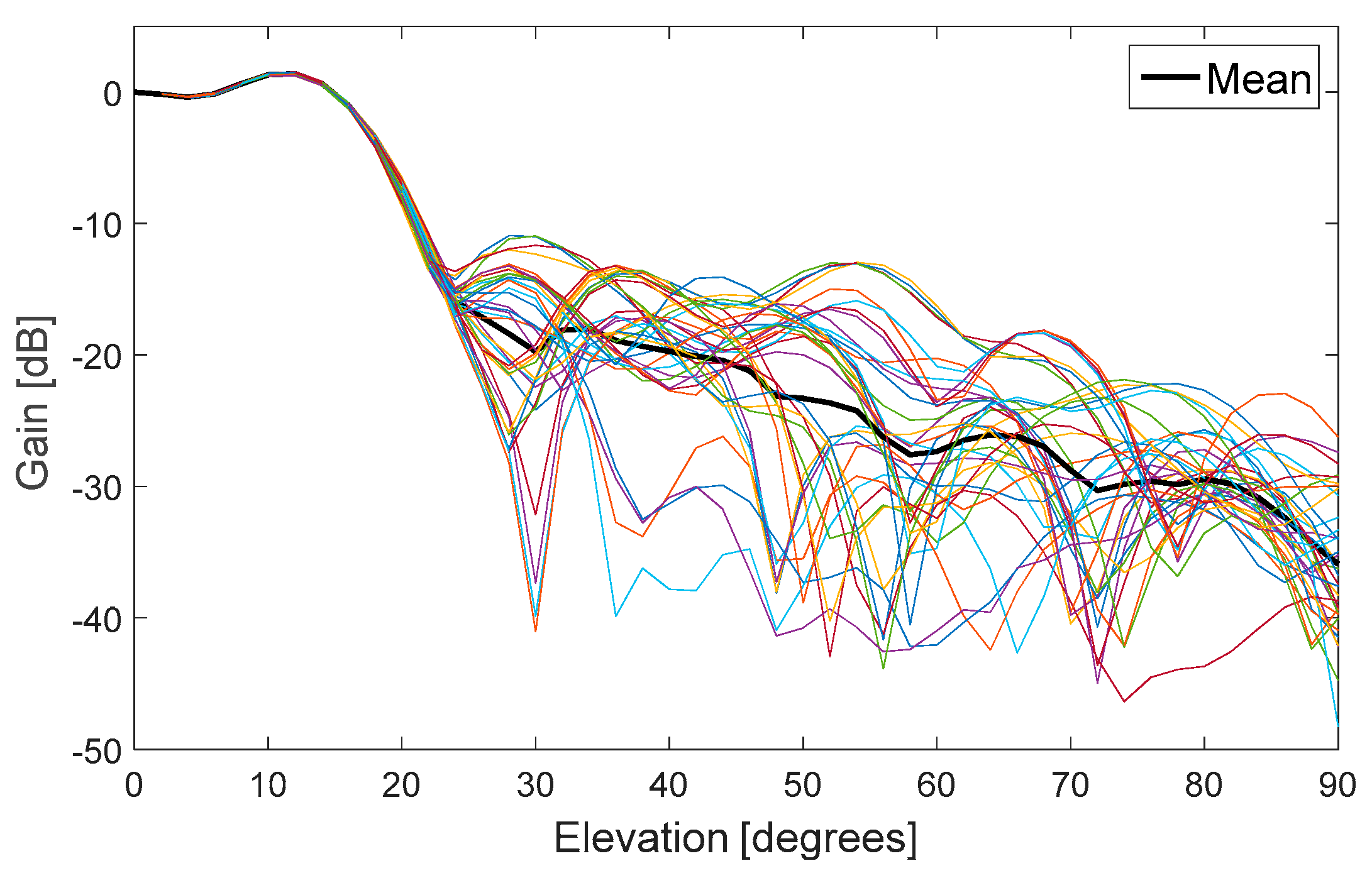
The published data in [3] for GPS L1 C/A Blocks IIR and IIR-M were used to model these blocks satellites’ antenna patterns. The measured antenna gain data and relative phase data for each transmitter of Block IIR and IIR-M are provided for L1 and L2 signals by Lockheed Martin in Appendix B and C of [3]. In [15], we can see that some of the IIR satellites use the legacy antenna pattern, while the remaining part and all the IIR-M satellites use the improved antenna pattern. For the benefit of terrestrial and space GPS users, the improved pattern includes a new design of the L-band elements mounted on the spacecraft’s Earth-facing structure. Meanwhile, for the GPS Block IIF satellites (built by Boeing), similar data have not been released. Logically, the antenna patterns used for GPS IIF Block should be at least as good as the improved antenna pattern used from Lockheed Martin. Thus, we decided to use a single 3D pattern for the satellites of Block IIF, where for each azimuth and each elevation the gain is the mean of the gains at the same azimuth and elevation of all the transmitters’ patterns with the improved antenna pattern in [15]. This pattern is illustrated in Figure 4, while in Appendix A of [3] all the gain patterns for each satellite of the IIR and IIR-M Blocks are shown.
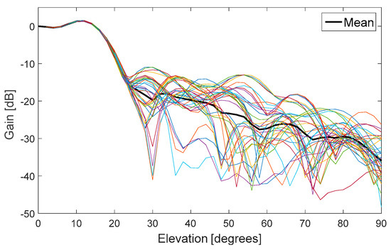
Figure 4.
Block IIF GPS L1 antenna gain pattern.
In the same figure is shown the assumed 2D antenna pattern for the satellites of Block IIF, which is the mean of the gains for different azimuth (in the same figure). In the same way the 2D patterns were formed for each satellite of block IIR and IIR-M from their respective patterns, shown in Appendix A of [3].
2.3.2. L5 Antenna Patterns
In this study three different options for the L5 pattern were used, approximated from the L1 patterns following the principle explained in [16]. We carried out a signal characteristics analysis for three different assumptions on the L5 antenna gain patterns:
- L5 antenna pattern 1. In the first case we modeled a different L5 antenna gain pattern for each satellite of IIR and IIR-M Blocks and only one L5 pattern for all the satellites of GPS IIF Block.
For each IIR satellite and IIR-M satellite we derived the L5 patterns from the GPS L1 assumed patterns as follows:
- (1)
- First, for each satellite, we computed a 2D pattern from the L1 detailed 3D pattern, where the gain for each elevation is the mean value of the gains for L1 for the same elevation and for all azimuths.
- (2)
- Second, maintaining the gain unchanged, we multiplied each elevation angle by a 1.1 factor.
Thus, essentially the 2D gain pattern of L5 differs from the one of L1 only in elevation.
To form the single L5 pattern used for all the IIF satellites from the L1 pattern, the same procedure was adopted.
- 2.
- L5 antenna pattern 2. In the second case we used the same pattern as the one defined for IIF satellites in the first case, for all GPS L5 satellites.
- 3.
- L5 antenna pattern 3. In this case we used the pattern provided in [5].
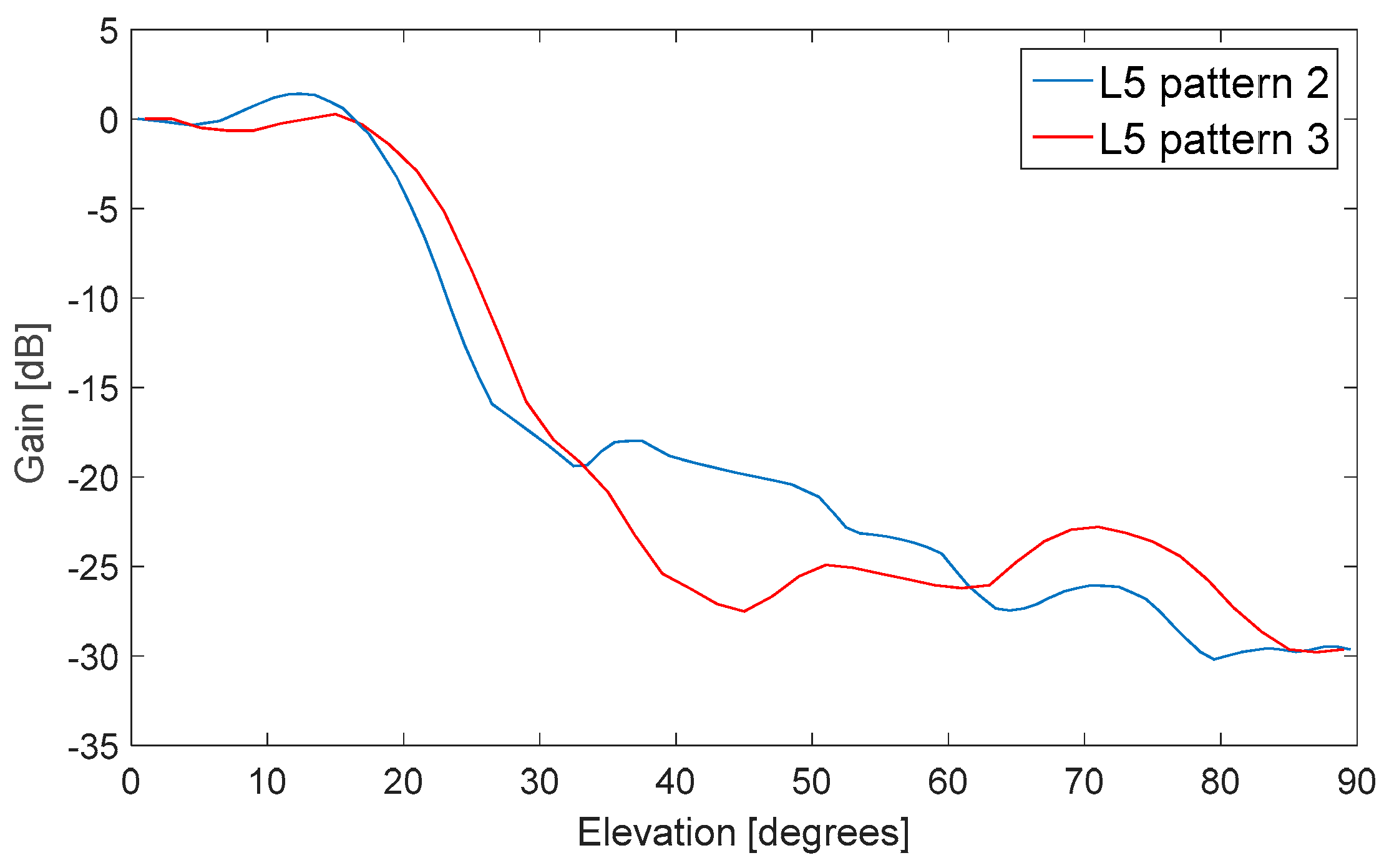
In Figure 5 is shown in blue the assumed L5 antenna gain pattern for the IIF satellites (in the first case) approximated from the L1 antenna gain pattern as explained above, also used in the second case for all GPS satellites. In red we can see the L5 antenna pattern 3.
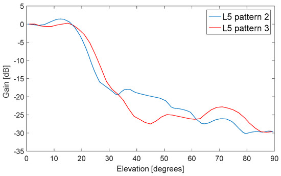
Figure 5.
GPS L5 antenna gain pattern.
3. Global Positioning System (GPS) L1 Receiver: 2D Pattern vs. 3D Pattern
The transmitters’ antenna patterns vary not only among the elevation, but also among the azimuth angles. This is also confirmed by the data made public in [3]. On one side the gain variation for the elevations used for terrestrial services is less than 1.5 dB, but, on the other side, this variation becomes very significant for the remaining part of the main lobe, and moreover it reaches values larger than 10 dB for the side lobes. Hence, the resultant performance when a signal is tracked at same elevation but at different azimuth would be different, especially for signals processed from the side lobes. However, due to a lack of precise antenna directivity data, in many research studies, this element is neglected. In most studies, a 2D antenna pattern is assumed, where the gain value is a function of the different elevations, but not of the different azimuth, for which an average value is assumed. In this case, the term in Equation (1) will be only function of the elevation .
In this context, this section aims at comparing quantitatively and qualitatively the GNSS performance obtained when assuming 3D antenna patterns with the one when 2D antenna patterns are considered.
3.1. Received Signal Power Levels
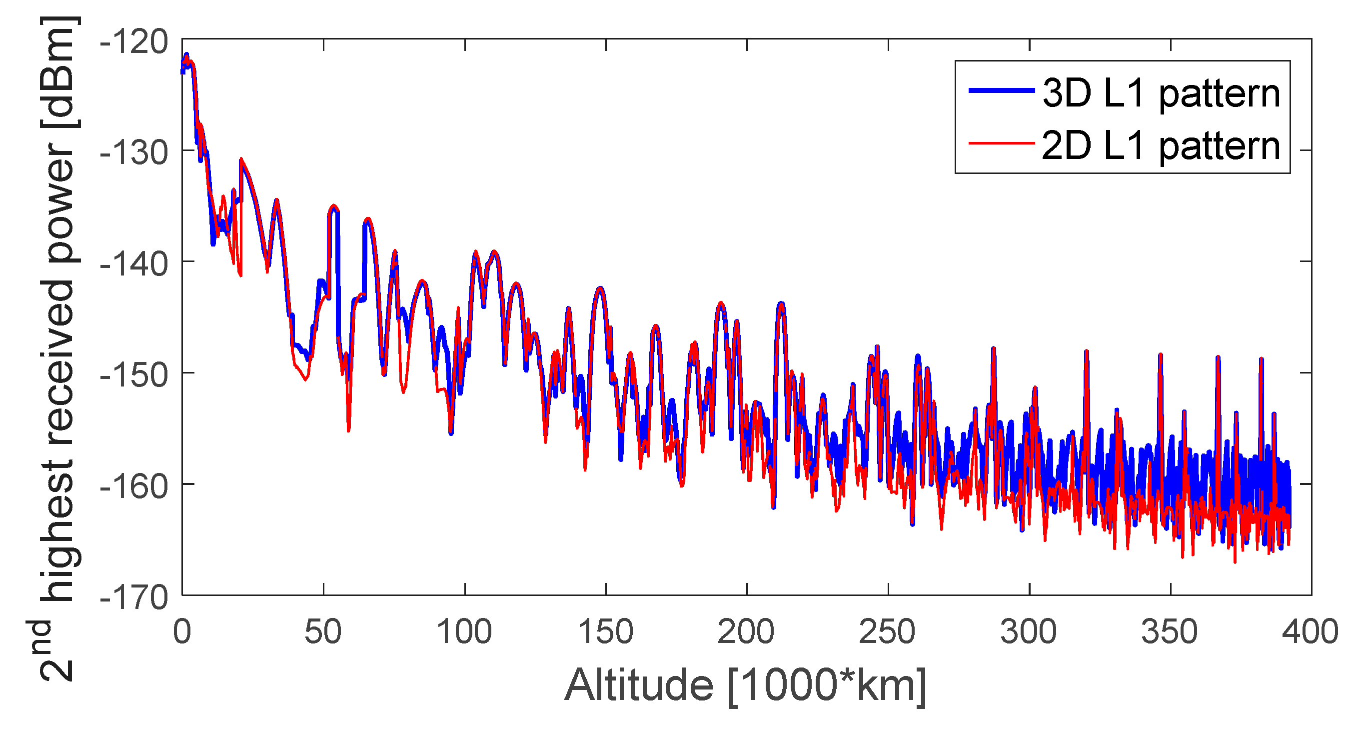
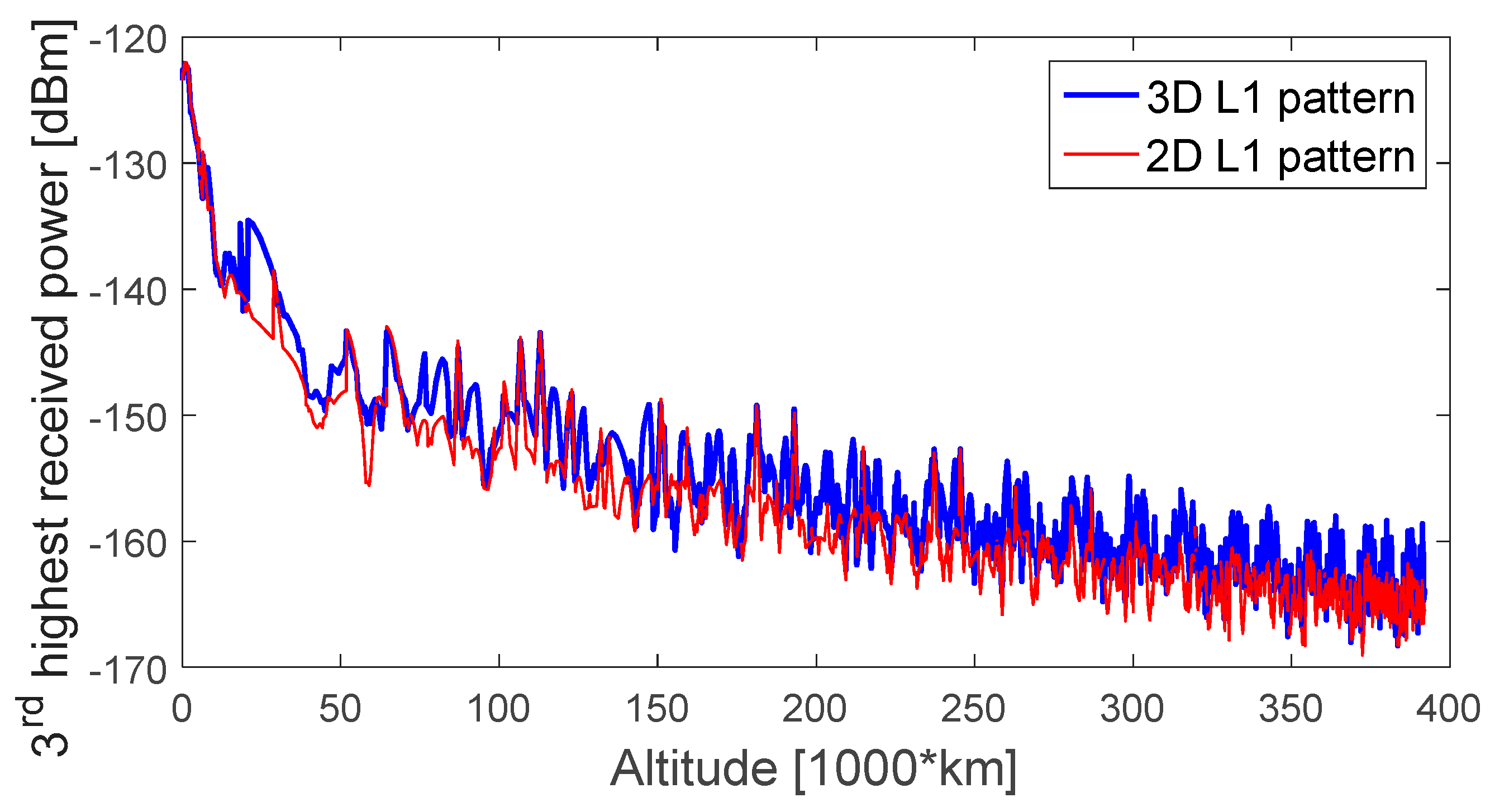
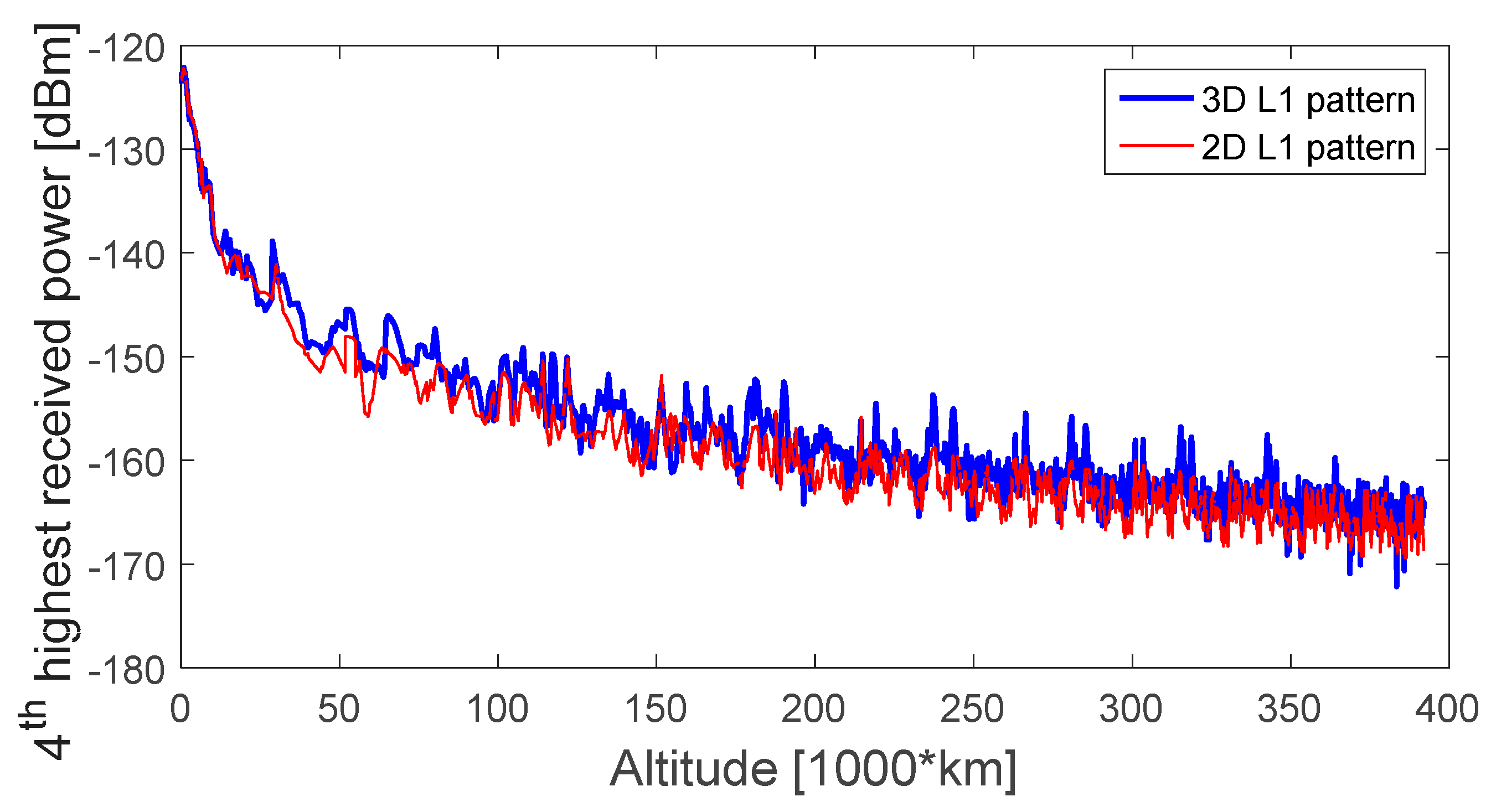
As a minimum of four signals are required for a standalone GPS navigation solution, Figure 6, Figure 7, Figure 8 and Figure 9 display the first-, second-, third-, and fourth-highest received power levels of the GPS L1 C/A signals at the receiver position as a function of the altitude, during the full considered trajectory, when assuming a 0 dBi receiver antenna gain, when the GPS L1 transmitter antenna is assumed to have a 3D pattern (in blue) and a 2D pattern (in red). The highest received signal powers (Figure 6) are very similar for both assumed patterns, which is explained by the fact that the signal comes from the main lobe of the transmitter antenna pattern; the main lobe patterns are very similar for 2D and 3D patterns, as also shown in Figure 4, because the main lobe pattern is well specified and there is a very small gain variance for different azimuth angles. The second-highest received signal powers reflect more differences, mostly at the end of the trajectory, as most of these signals come from the side lobes, where the dependency of the transmitter’s antenna gain with the azimuth is more evident; the differences are more notable in the case of the third-highest received power during the entire MTO.
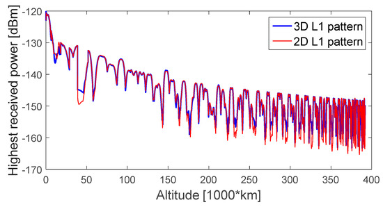
Figure 6.
Highest received power level of GPS L1 signals, during the considered MTO, for a 0 dBi receiver gain pattern.

Figure 7.
Second-highest received power level of GPS L1 signals, during the considered MTO, for a 0 dBi receiver gain pattern.

Figure 8.
Third-highest received power level of GPS L1 signals, during the considered MTO, for a 0 dBi receiver gain pattern.
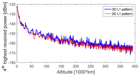
Figure 9.
Fourth-highest received power level of GPS L1 signals, during the considered MTO, for a 0 dBi receiver gain pattern.
As with four signals we would be able to compute the navigation solution, the fourth received signal power is of highest interest for us. What we can notice from Figure 9 is that in the case of 3D pattern the fourth-highest received signal power is sometimes lower than −170 dBm. On the other hand, this is never the case for the 2D pattern. Observing Figure 9 carefully, we can notice that the received powers are different; however, it is hard to have clear evidence, in which case the received powers are higher. For a better understanding of the effect of the two considered patterns, in the next section we will investigate the signals’ availability.
3.2. Availability and Geometric Dilution of Precision (GDOP)
In this study the i-th GPS observation is considered available if the corresponding i-th GPS L1 C/A signal is acquired and tracked. According to the capability of the SANAG receiver, the i-th GPS L1 C/A signal:
- Is acquired if the corresponding signal power is equal to or stronger than 20 dB-Hz without any interruption in the time interval , or if it is weaker than 20 dB-Hz but stronger than 15 dB-Hz without any interruption in the time interval .
- Is tracked if the corresponding signal power is equal to or stronger than 15 dB-Hz.
Note that once the receiver is orbiting above the ionosphere upper bound, the few GPS L1 C/A signals that cross the ionosphere are discarded, since they may be affected by large ionospheric delay due to the double crossing of the ionosphere.
Figure 10 illustrates the availability of satellites as a function of the altitude, during the full considered trajectory, for both considered antenna patterns, assuming 10 dBi receiver antenna gain.
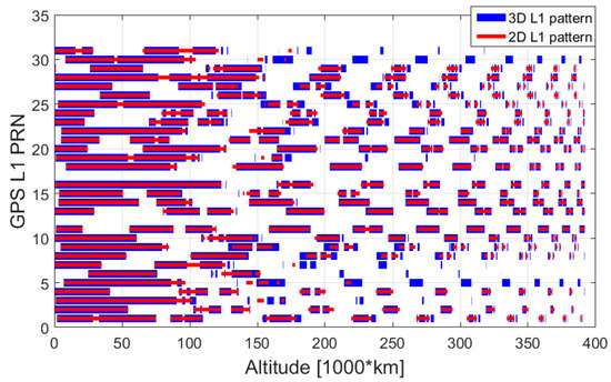
Figure 10.
Available GPS L1 signals, during the assumed MTO, for a 10 dBi receiver gain pattern.
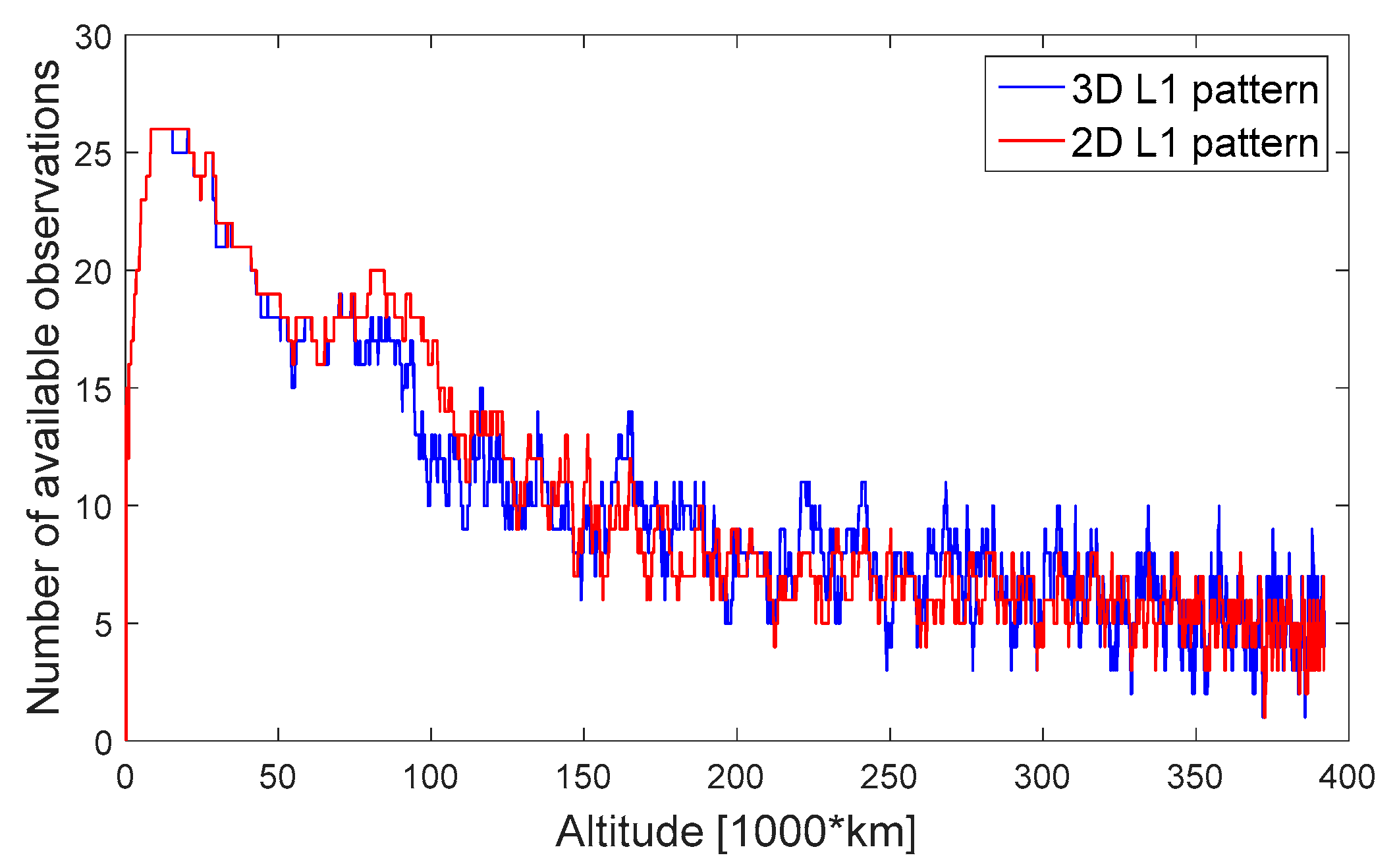
From this plot we cannot conclude for which pattern the availability is higher, however we can see that when assuming a 3D pattern it happens much more often to lose a satellite for a short time and track it again shortly after, compared to the case when we are using a 2D pattern. This is expected as, in the case of a 3D pattern, the gain might change a lot for different azimuth, more often causing a sudden loss of sight on a satellite. Another way to distinguish the impact of averaging the antenna pattern on the availability is to plot the total number of observations available, as shown in Figure 11. From this plot we can see that, depending on the portion, the availability might be higher for either a 3D or a 2D pattern. However, it is interesting to notice that in the case of a 2D pattern after 200,000 km altitude, the number of satellites available has a lower standard deviation compared to using a 3D pattern. Hence, in the case of a 3D pattern there are more outages, as well as more peaks in the number of satellites. The precise statistics on the availability are computed for the entire MTO as well as for three representative portions, as defined in Table 2. They are reported in Table 3, where the two assumed patterns are more concretely compared.

Figure 11.
Number of available observations during the assumed MTO.
Table 2.
Definition of representative portions.
Table 3.
Statistics for the number of available observations.
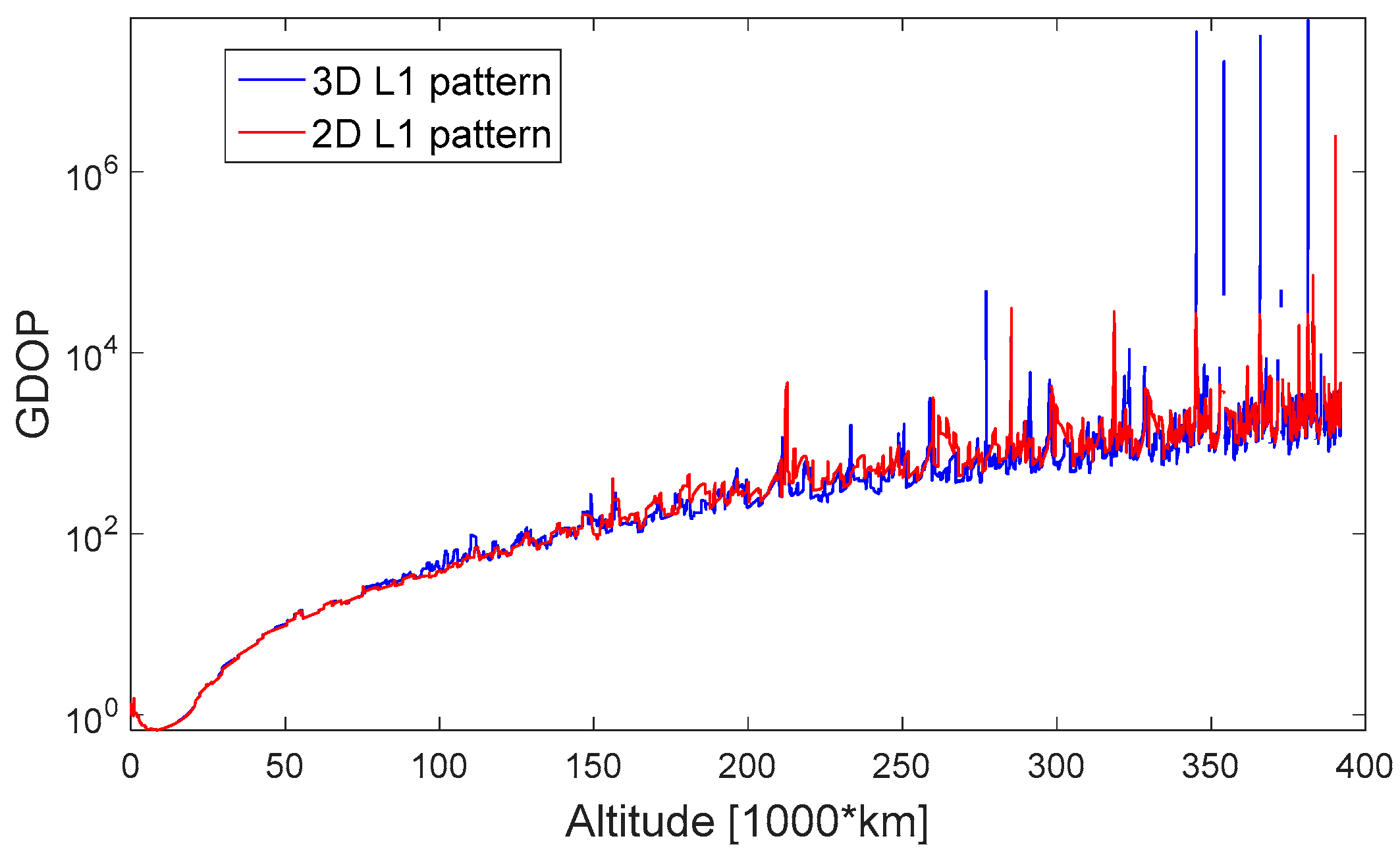
In Figure 12, the GDOP is shown. From this figure, it is difficult to assess which between the 3D or the 2D pattern leads to the worst GDOP; in some portion the 3D pattern has higher GDOP and in some other portions lower GDOP. However, at the end of the MTO for the 2D pattern the GDOP reaches its maximal value of 2.5 × 10⁶, while, when we assume a 3D pattern, there are much more important peaks with a maximum of about 4.7 × 10⁷, as shown in Figure 12.
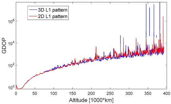
Figure 12.
Geometric dilution of precision (GDOP) in log scale during the assumed MTO.
In Table 3 the statistics of the availability are reported for the three representative 500 min portions (as defined in Table 2) of the trajectory and during the full trajectory, for both assumed patterns. As we can see in the first portion, the availability is slightly higher when assuming a 2D pattern; however, in the second and third portion assuming a 3D pattern would result in slightly higher availability. Finally, as expected, averaging the pattern results in different availability, although not significant; for instance, considering the full trajectory, the difference is less than 1% or less than 0.2 satellites observed on average per epoch (1 s).
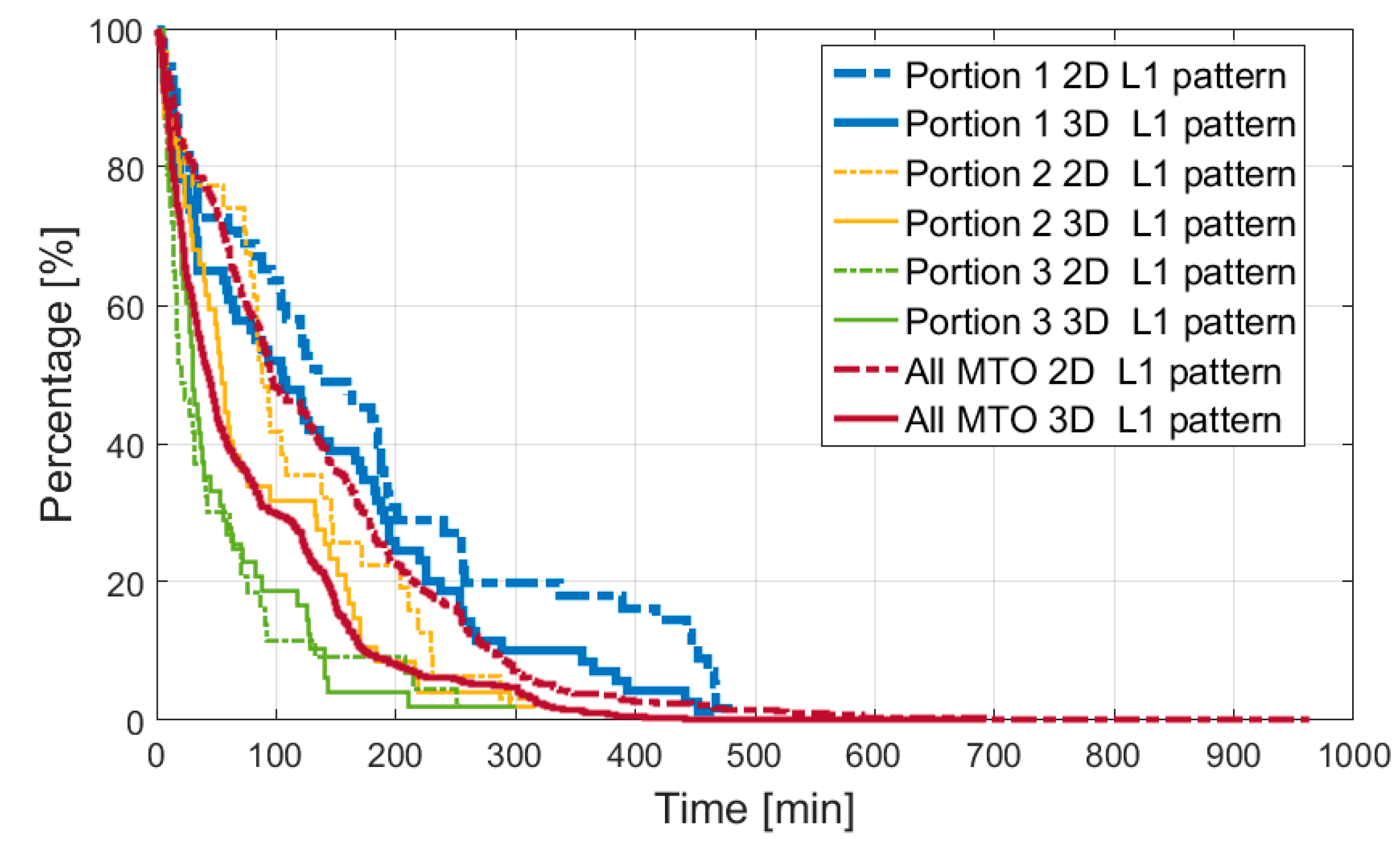
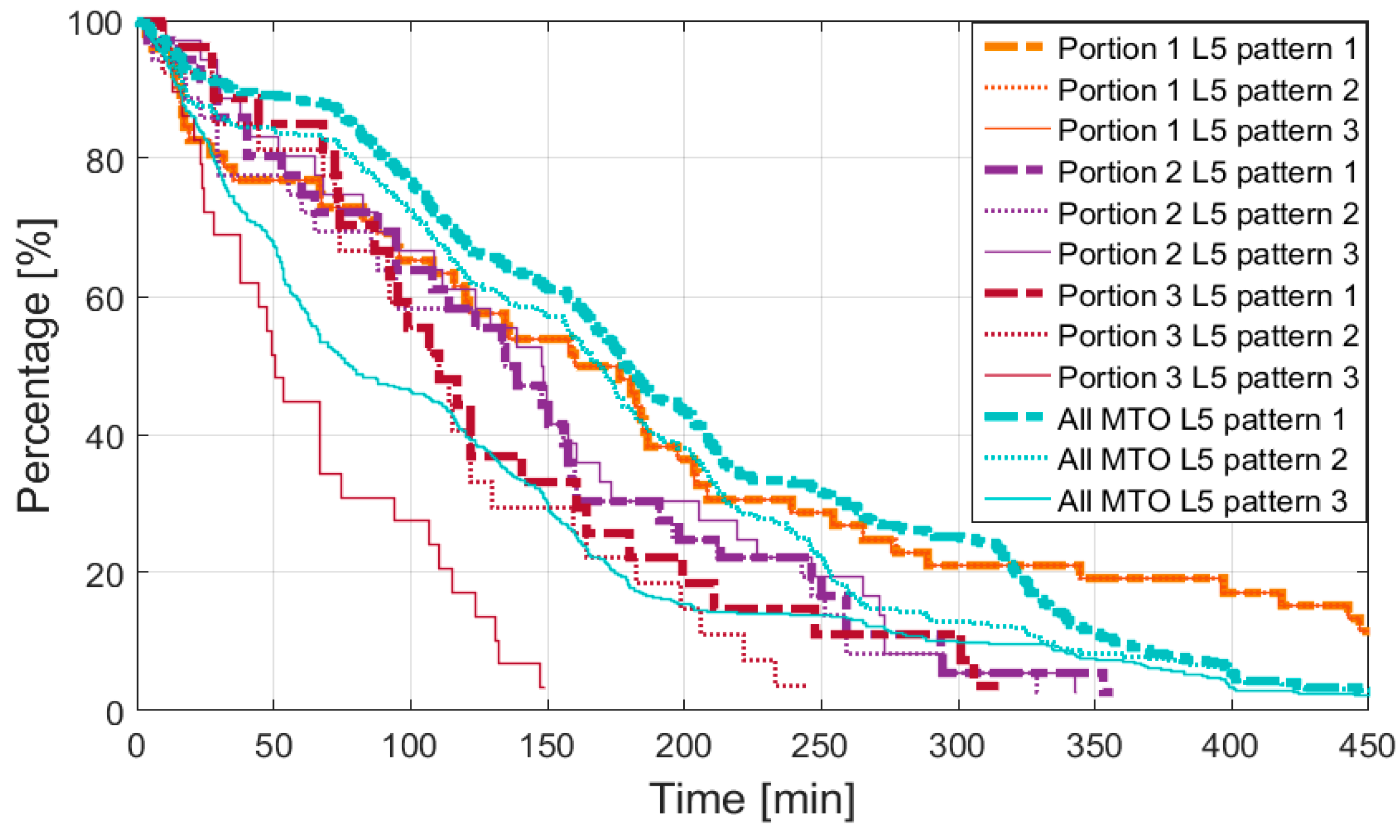
Another important piece of information related to the availability is the continuity of the signal as time interval duration when the signal is continuously available. This information is very useful for the acquisition module design. The continuity can be expressed in terms of percentage of continuous time intervals with the duration equal to or longer than a time interval T. This is shown in Figure 13 for both assumed patterns, for the full trajectory and the defined portions.
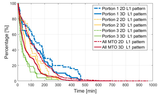
Figure 13.
Percentage of continuous time intervals, a point of each curve identifies a time interval duration T (on the x-axis) and the corresponding percentage (on the y-axis) of continuous time intervals equal or longer than T.
3.3. Ranging Error
This section focuses on the impact of the two different assumed antenna patterns on the pseudorange error. The pseudorange error is the sum of different errors affecting the measurement, as we can see from Table 1. In this study, all the pseudorange errors were modeled as in our previous study [9]. However, it is relevant to mention here that, assuming the use of code based observations (as for the SANAG receiver), the code tracking thermal noise error is the main error affecting the pseudorange whose standard deviation can change over time due to a different signal power level at the receiver position, and then due to a different transmitter’s antenna pattern model. Hence, for the two considered antenna patterns, for simplicity, we only report the simulated code tracking thermal noise.
According to [17], for binary phase shift keying (BPSK) modulations, the thermal noise code tracking jitter is:
with the code loop noise bandwidth (in Hz), the early-to-late correlator spacing (in chips), the coherent integration time (in s), the double-sided front-end bandwidth (in Hz), the chipping rate (in chips/s) and the carrier to noise ratio (in dB-Hz). In this work we assumed: = 0.1 Hz and = 20 ms for both signals; = 0.25 chips for L1 and = 0.8 chips for L5; = 13 MHz for L1 and = 40 MHz for L5.
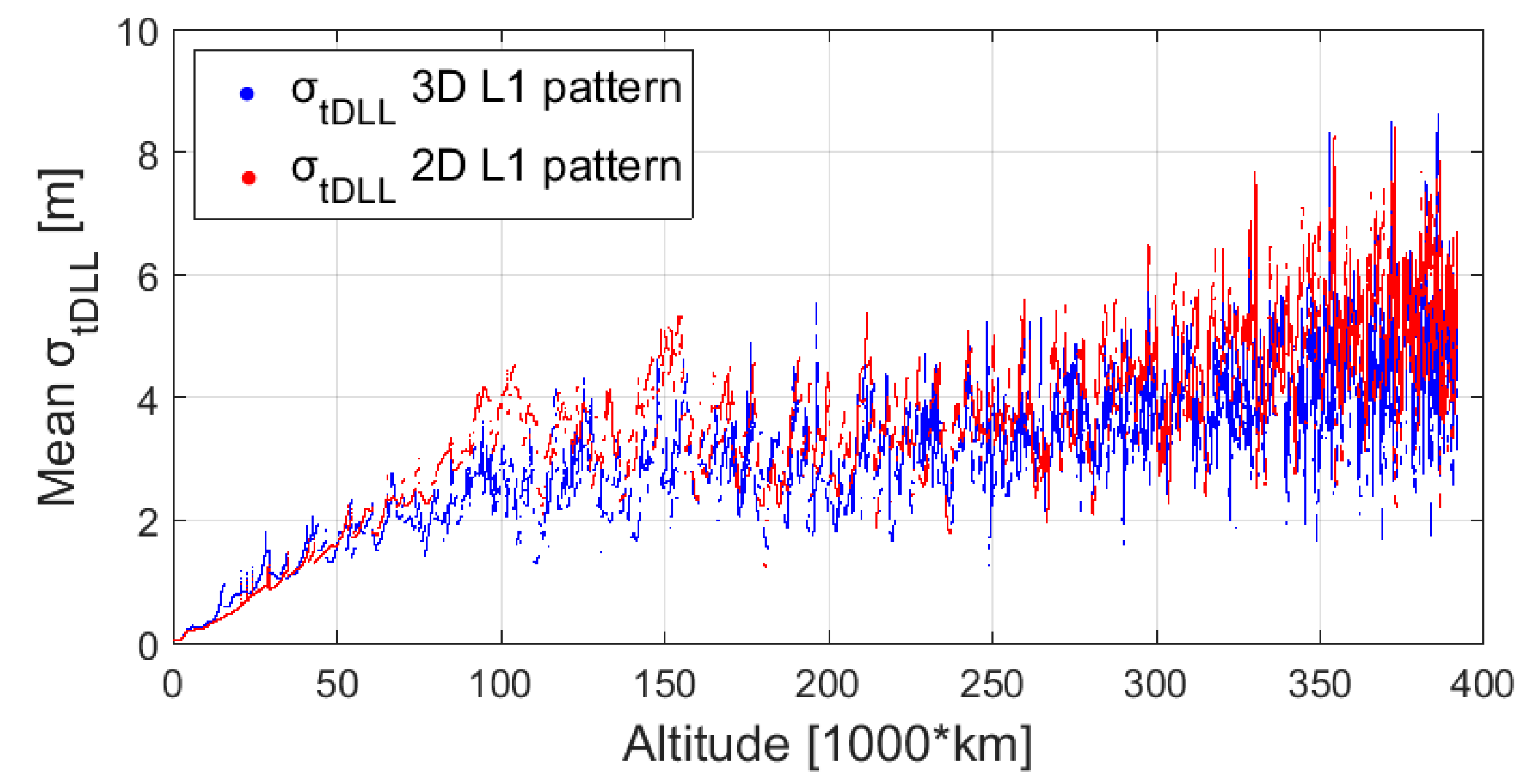
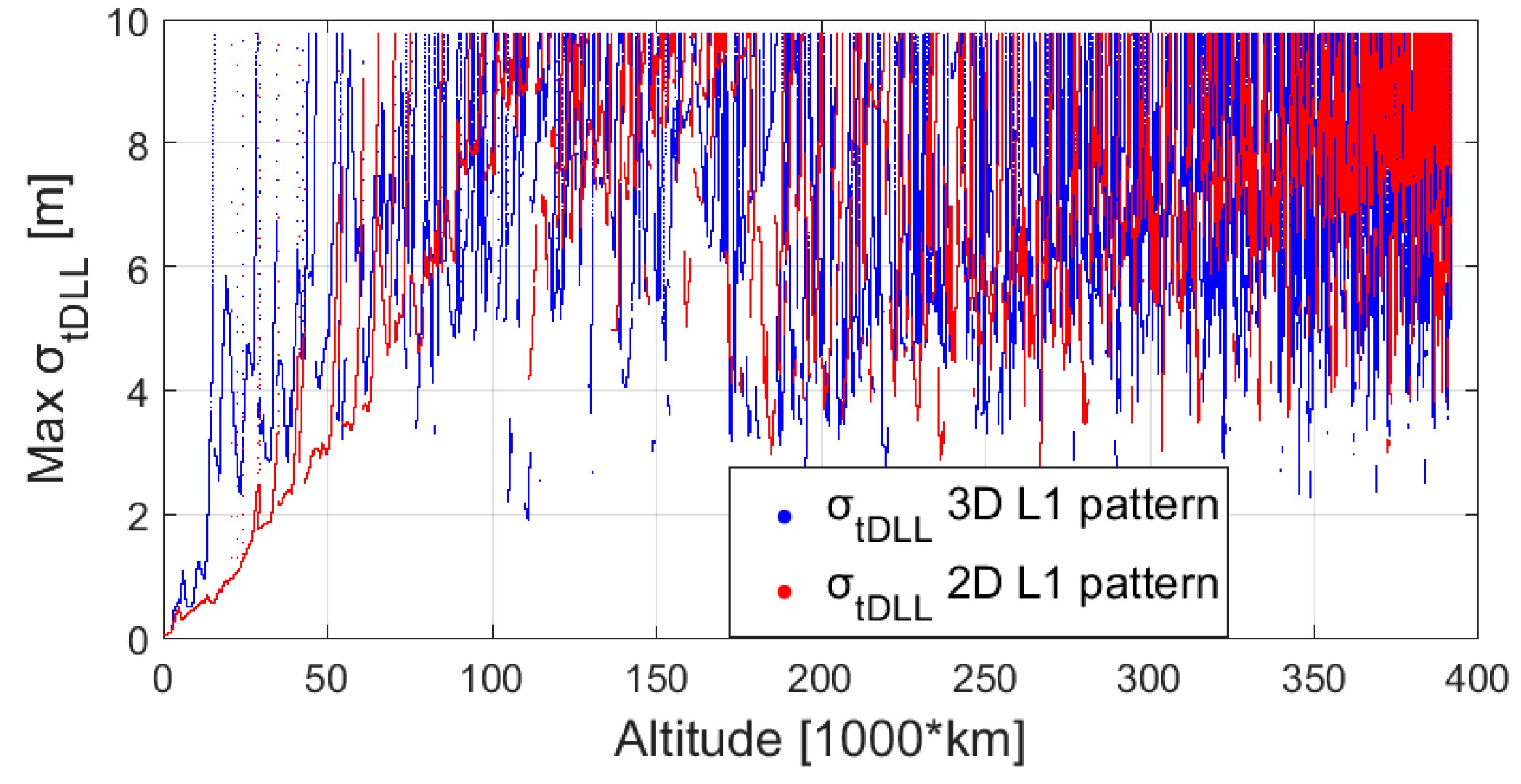
Figure 14 and Figure 15 show respectively the mean and max , assuming 10 dBi antenna gain for the receiver. The mean and max code tracking thermal noise error are computed among the signals available at the same instant. For instance, the for each available signal is displayed in Figure 16 in case of the 3D L1 antenna pattern assumption, as a function of the altitude. We can see from Figure 14 that it is difficult to state which antenna pattern (3D or 2D) would result in higher thermal noise, and thus ranging error. For example, at the beginning of the trajectory, up to 60,000 km, using the 3D pattern would bring a higher thermal noise, however from 75,000 km to 160,000 km using the 2D pattern would result in higher thermal noise. Finally, based on these results, using a 2D or 3D pattern would result in different for each pseudorange; however, when computing the mean , the difference becomes small. From Figure 15 we can notice that at the beginning of the trajectory, up to 50,000 km the maximal would be higher when assuming a 3D L1 pattern. It is important to note that the for both 3D and 2D patterns does not exceed a certain value (approximately 10 m), which corresponds to the weakest signals that the receiver can process due to its limited sensitivity.
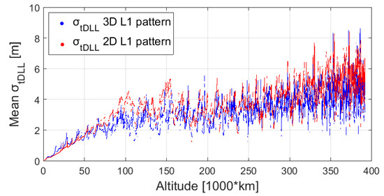
Figure 14.
Mean code tracking thermal noise range error, for the assumed MTO. The thermal noise range error is computed for each available pseudo random noise (PRN) and the mean is plotted.

Figure 15.
Max code tracking thermal noise range error, for the assumed MTO. The thermal noise range error is computed for each available PRN and the max is plotted.
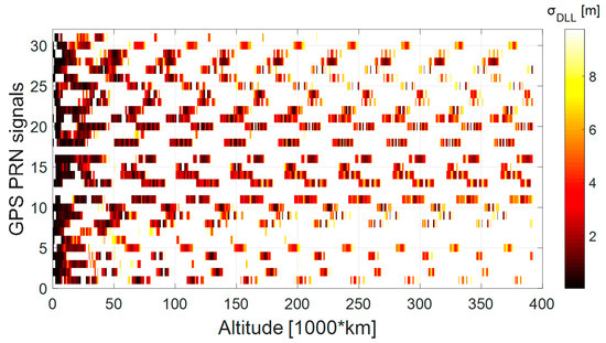
Figure 16.
, when assuming 3D transmitter patterns.
3.4. Navigation Solution
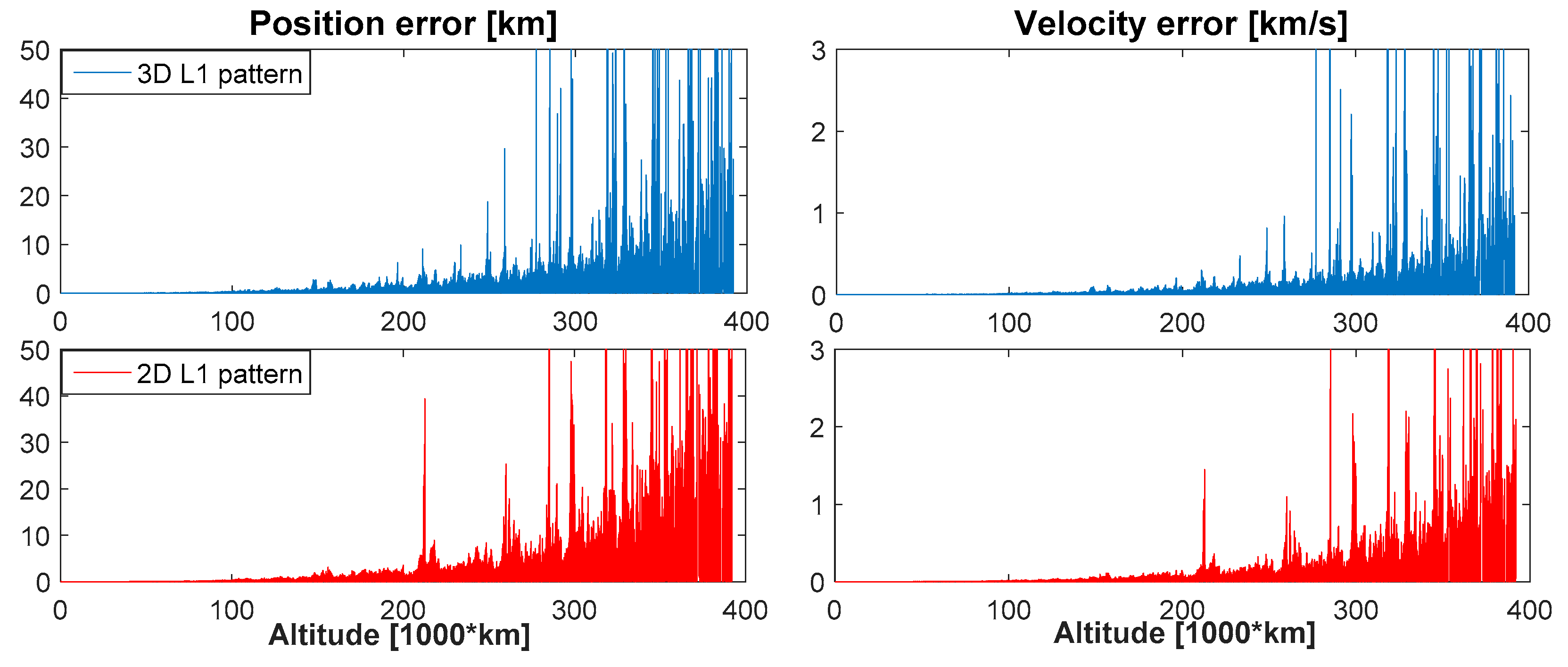
In this section the impact on the navigation solution when assuming a 2D L1 antenna pattern and a 3D L1 antenna pattern are compared. Initially the impact on the standalone GPS navigation solution is evaluated. In this case, we computed the single-epoch least squares position and velocity estimation errors. The accuracy given by unfiltered single-epoch least squares estimations would be very coarse at Moon altitude, not fulfilling the mission requirements. Indeed, at Moon altitude, the relative geometry between the GPS satellites and the receiver (very high GDOP values) is very poor and the ranging errors (user equivalent range error (UERE)) can be significant (due to the low signal powers).
As presented in our previous works [7,9], we used an adaptive orbital filter to process the GNSS measurements using a model of the orbital forces acting on the hosting spacecraft. The GNSS measurements processed by the filter, can be position and velocities or directly pseudoranges and pseudorange rates. The measurements and the predicted measurements have different error distributions, leading to an improved navigation solution compared to the ones obtained individually. A detailed implementation of the orbital filter is presented in [7]. Therefore, in addition to evaluating the effect of assuming a 2D L1 pattern or a 3D L1 pattern on the single-epoch least squares solution, it is useful to estimate the same effect on the filtered navigation solution as well.
3.4.1. Least Squares Estimation
In Table 4 the navigation solution statistics are shown, while Figure 17 illustrates the zoomed navigation solution for the two assumed patterns. Looking at Figure 17, we can see that the performance is quite similar for both cases; however, according to Table 4, using a 2D pattern would result in better navigation performance for the full MTO; on the other hand, looking at the statistics of each evaluated portion using a 3D pattern results generally in better statistics. This is only true because of a few points where the GDOP considerably affects the navigation solution in the case of a 3D pattern. Indeed, as already mentioned in Section 3.2, the number of observations available when using a 3D pattern has a higher standard deviation, leading to a larger number of outages (as well as more peaks in the number of satellites), which causes a very bad relative geometry between the transmitters and the receiver. Indeed, the maximal GDOP for the 2D pattern is 2.5 × 10⁶, while for the 3D pattern it is 4.7 × 10⁷ and the GDOP has more peaks in case of the 3D pattern compared to the 2D one.
Table 4.
Statistics of the single-point least squares estimation error.

Figure 17.
Single-point least squares estimation error for the assumed MTO.
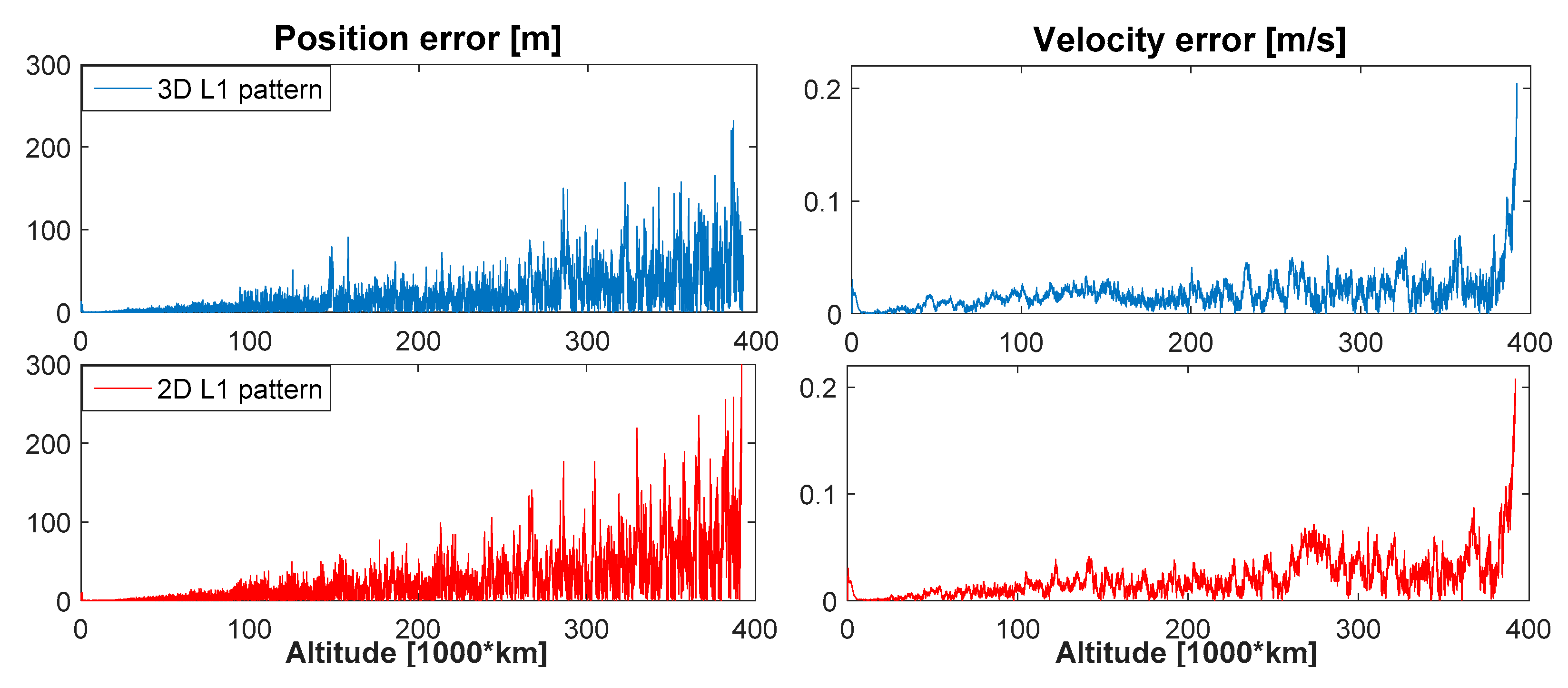
3.4.2. Range-Based Orbital Filter
Figure 18 shows the navigation solution obtained when processing GPS L1 pseudoranges and pseudorange rates by means of the implemented orbital filter. We can see that, unlike when we compute the position and velocities with a least squares estimator, when using the filter, the results obtained assuming a 2D antenna pattern are very similar to the ones obtained assuming a 3D antenna pattern. The exact statistics are shown in Table 5. In particular, the difference in velocity estimation errors never exceeds 0.011 m/s. For the position estimation error, the mean and the standard deviation have a maximum difference of about 0.4 m in the first portion, 6 m in the second portion, 1 m in the third portion, and 9 m for the entire MTO, while the difference in maximum is more important (more than 50 m for the entire MTO).
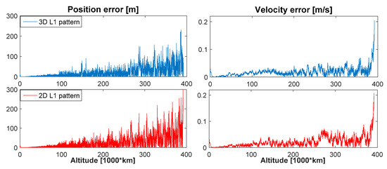
Figure 18.
Range-based orbital filter estimation error for the assumed MTO.
Table 5.
Statistics of the range-based orbital filter estimation error.
4. GPS L1/L5 Receiver: L5 Pattern Assumption
Lack of information on the L5 antenna pattern has always been a big struggle for engineers trying to design a spaceborne receiver. The only information known is that the main lobe is wider than the one of the L1 pattern [2]. In this sense it can be approximated from the L1 pattern using the ICD document [4,14], but on the other side, the side lobes approximation is less accurate. Indeed, while the main lobe has almost the same gain values for different azimuth of the same satellite, and furthermore for different satellites, the side lobes do not. Hence, this makes the assumption of the L5 pattern, especially for side lobes, very important, as it might affect the results. In this context, here, we want to evaluate the effect of assuming the different L5 antenna patterns defined in Section 2.3 on the GNSS availability and the GNSS-based navigation performance.
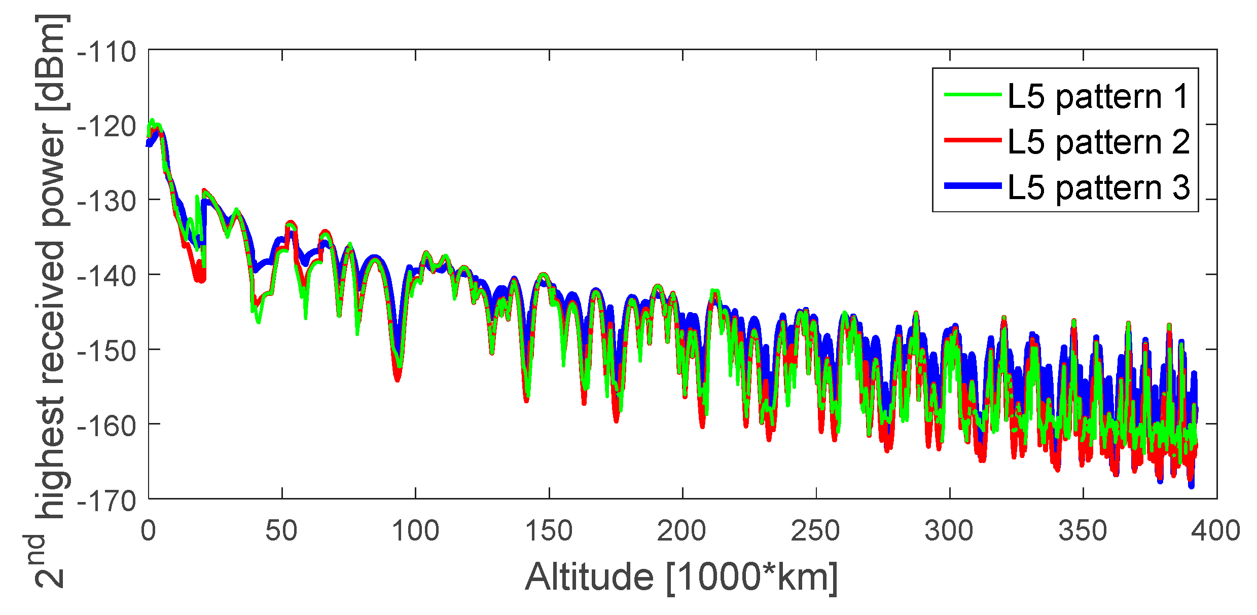
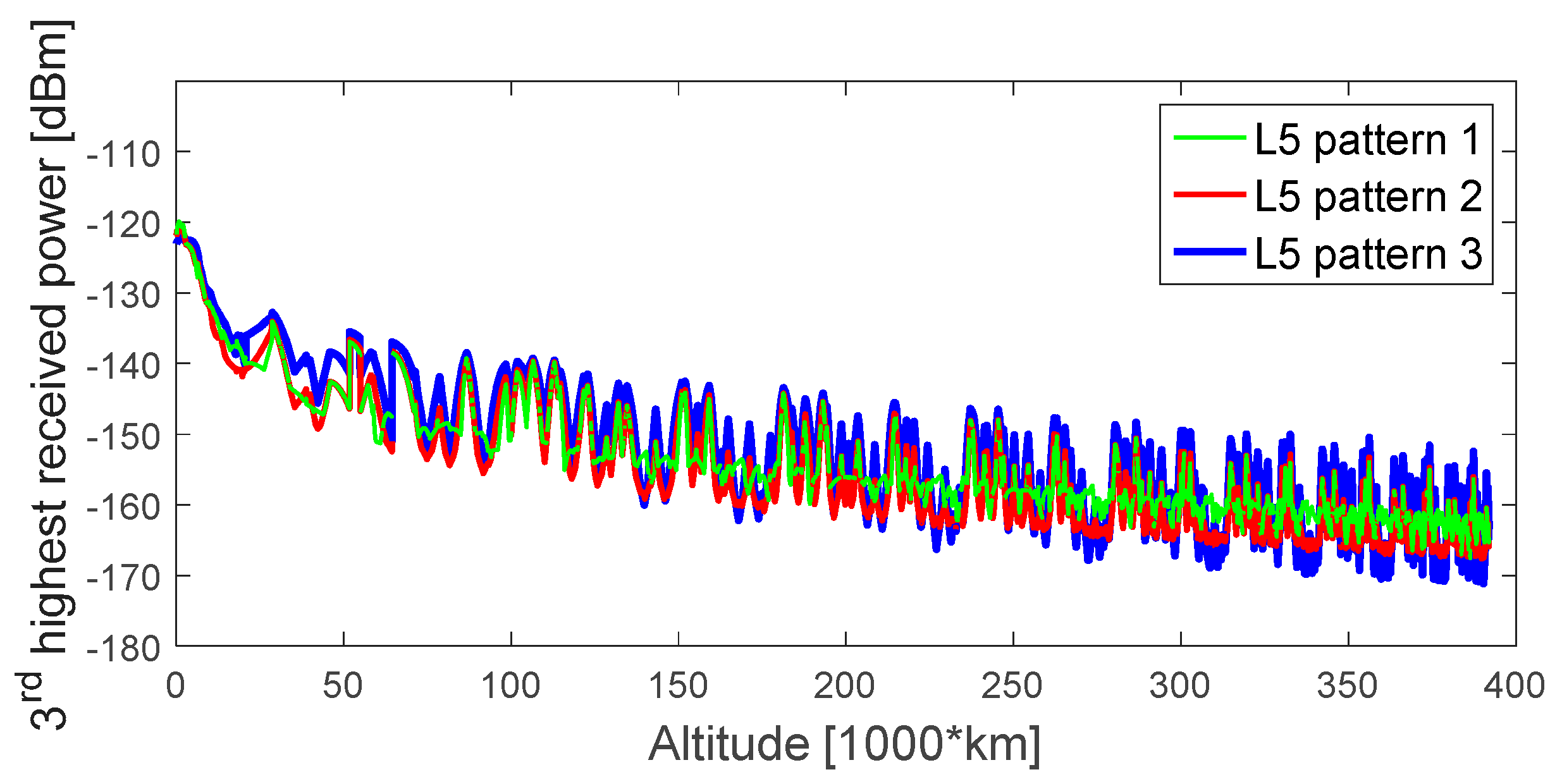
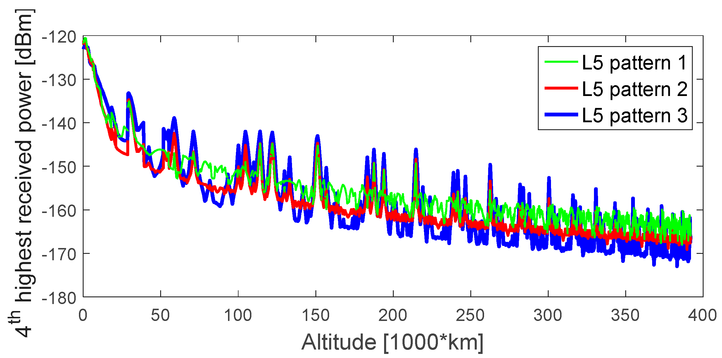
4.1. Received Signal Power Levels
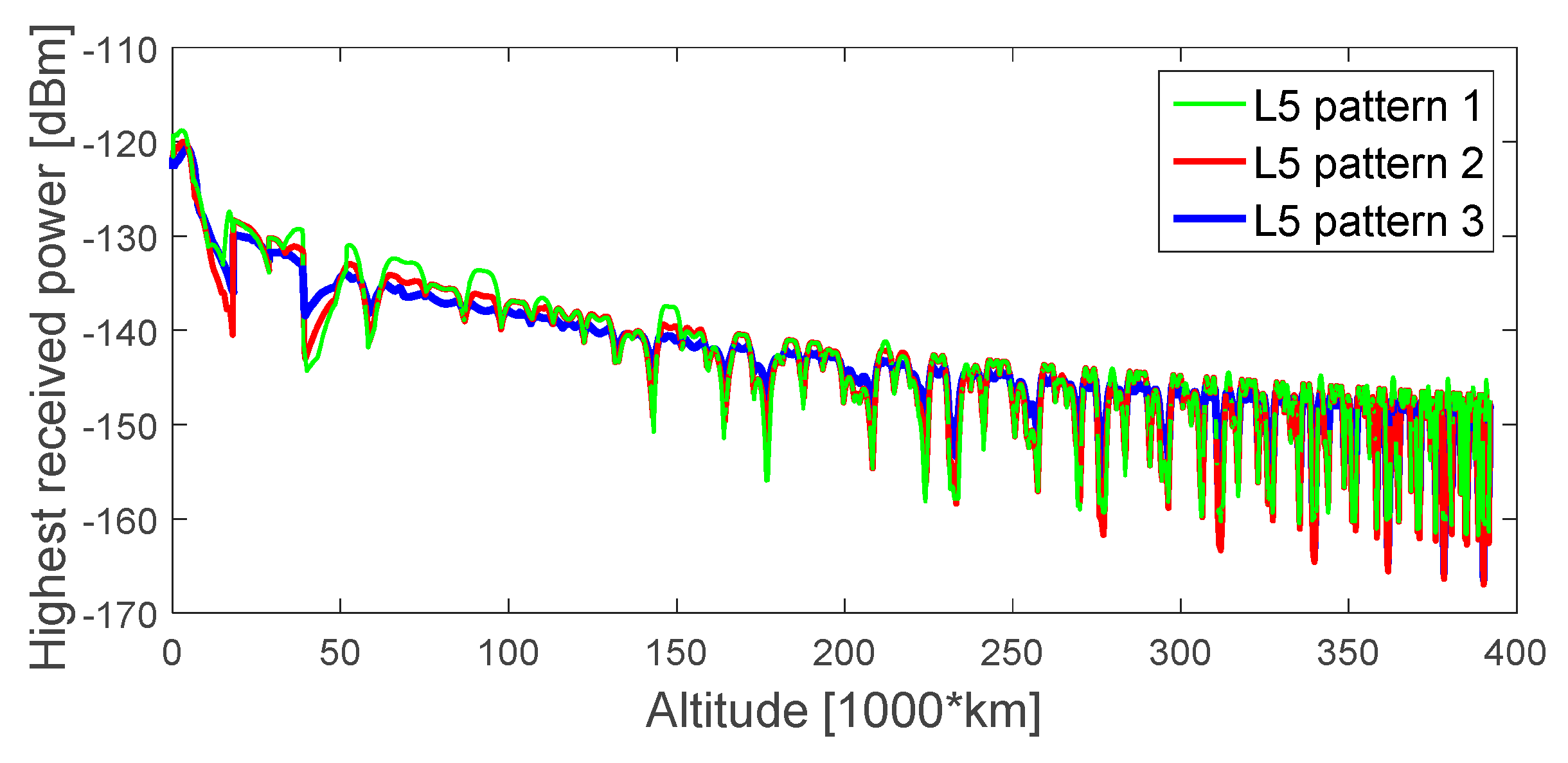
Figure 19, Figure 20, Figure 21 and Figure 22 show the four highest received power levels of the GPS L5Q signals at the receiver position as a function of the altitude, during the full considered trajectory, when assuming a 0 dBi receiver antenna gain, for the three assumed L5 antenna patterns. As we can see from these figures, the highest and the second-highest received signal powers have similar plots for the three assumed L5 patterns, while the third- and fourth-highest received signal powers plots are more different. From the four figures, we can notice that assuming L5 pattern 1 would result in higher received signal powers, always at the end of the MTO, and also in general for the fourth-highest received power. Again, the most important plot is the fourth-highest received power, in order to have at least four signals, and therefore to be able to compute the navigation solution. From Figure 22 we can see that when assuming L5 pattern 1 the signal power level is never smaller than −169 dBm; when assuming L5 pattern 2 it goes below −169 dBm at a few points at the very end of the trajectory; and when assuming L5 pattern 3 the received signal power level is below −169 dBm for a considerable amount of time after 310,000 km altitude. Moreover, most of the time, the highest fourth signal power has higher values in the case of L5 pattern 1, while it has lower values in case of L5 pattern 3 for most of the time. In the next session we will investigate the signals’ availability, in order see the impact of the three assumed L5 patterns.

Figure 19.
Highest received power level of GPS L5 signals, during the considered MTO, for a 0 dBi receiver gain pattern.
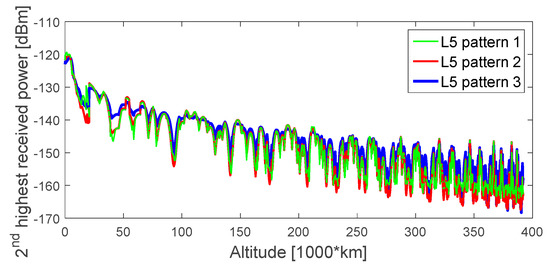
Figure 20.
Second-highest received power level of GPS L5 signals, during the considered MTO, for a 0 dBi receiver gain pattern.

Figure 21.
Third-highest received power level of GPS L5 signals, during the considered MTO, for a 0 dBi receiver gain pattern.
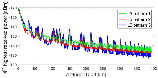
Figure 22.
Fourth-highest received power level of GPS L5 signals, during the considered MTO, for a 0 dBi receiver gain pattern.
4.2. Availability and GDOP
In this case, according to the dual frequency L1/L5 capabilities of the SANAG receiver, the i-th GPS observation is considered available at time if:
- At time , the corresponding i-th GPS L1 C/A signal is acquired (i.e., according to the conditions already specified in Section 3.2).
- In case the i-th GPS signal does not cross the ionosphere: the corresponding i-th GPS L5Q signal is tracked (i.e., the corresponding signal power is equal to or stronger than 12 dB-Hz).
- In case the i-th GPS signal crosses the ionosphere: the corresponding i-th GPS L5Q and GPS L1 C/A signals are both tracked (i.e., the corresponding signal power is equal to or stronger than 12 dB-Hz for GPS L5Q and 15 dB-Hz for GPS L1 C/A).
In Figure 23 is illustrated the availability of satellites as a function of the altitude, for the three considered L5 antenna patterns, during the entire MTO, assuming 10 dBi antenna gain for the receiver.
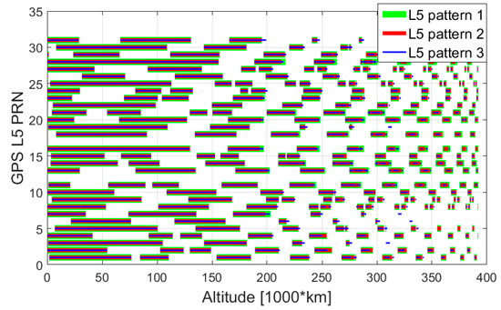
Figure 23.
Available GPS L5 signals, during the assumed MTO, for a 10 dBi receiver gain pattern.
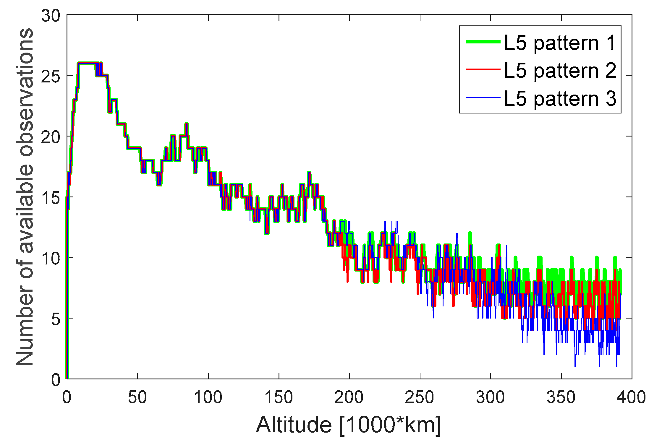
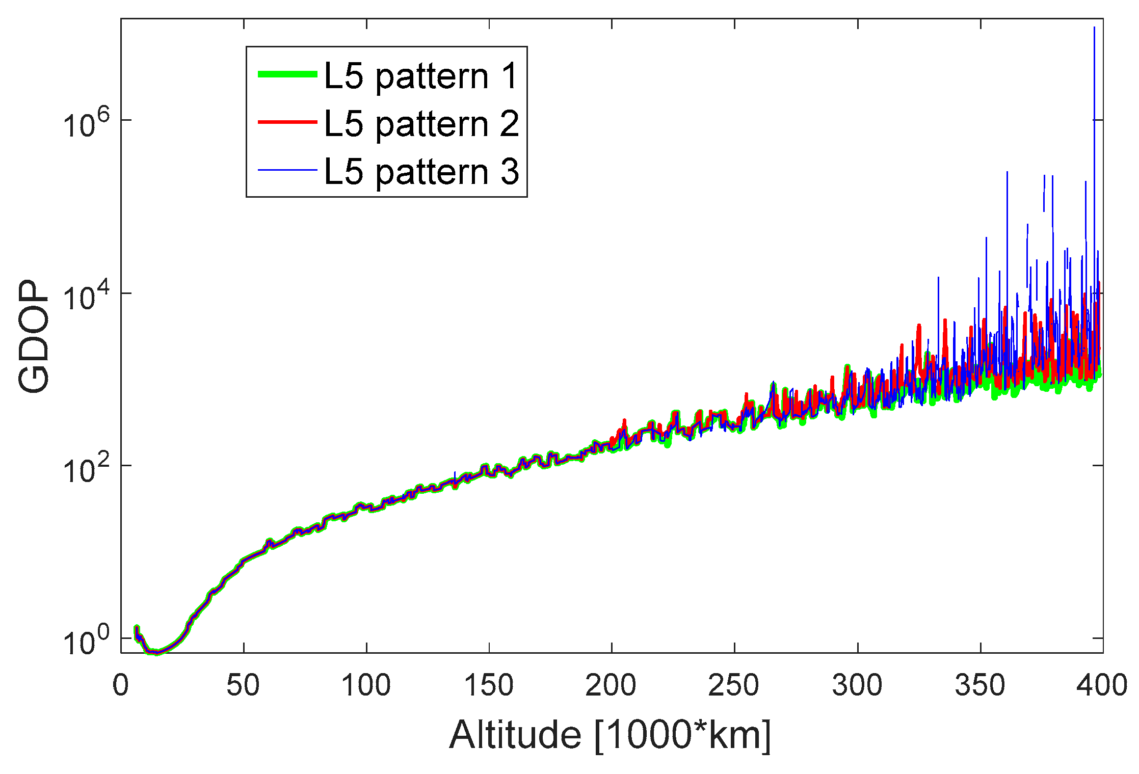
The total number of available observations at each altitude is shown in Figure 24, where we can see clearly that at the end of the trajectory the availability is lower when assuming L5 pattern 3. Indeed, in this case, at the end of the considered MTO, the number of available observations is often less than 4, which is never the case for the other two assumed patterns (i.e., L5 pattern 1 and L5 pattern 2). Table 6 reports the precise information on the availability for the full trajectory and the three considered representative portions, such as percentage of availability, mean, max, and min number of available satellites, and percentage of time when more than four satellites are available. The GDOP for the three considered L5 patterns is shown in Figure 25. What is interesting to notice is that up to 250,000 km the GDOP has similar values for the three considered cases. As displayed in Figure 25, in the case of L5 pattern 3, the GDOP very often reaches values larger than 10,000 (at the end of the MTO).

Figure 24.
Number of available observations during the assumed MTO.
Table 6.
Statistics for the number of available observations.
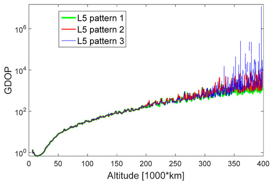
Figure 25.
GDOP in log scale during the assumed MTO.
Meanwhile, the continuity in terms of percentage of continuous time intervals with a duration equal to or longer than time interval T is shown in Figure 26 for the full MTO and the three considered portions. We can see that for the first portion the continuity curves are almost the same for the three considered L5 patterns, while for the two other portions and the entire trajectory they are different.

Figure 26.
Percentage of continuous time intervals, a point of each curve identifies a time interval duration T (on the x-axis) and the corresponding percentage (on the y-axis) of continuous time intervals equal or longer than T.
From Table 6 we can conclude that the third assumed L5 (i.e., L5 pattern 3) patterns leads to worse availability mainly in the third considered portion compared to L5 pattern 1 and L5 pattern 2. Indeed, in this portion, the availability for L5 pattern 3 is almost half that for the other two patterns, which is reflected in the mean number of satellites, 7.13, 6.21, and 3.74, respectively, for the first, second, and third assumed L5 patterns. For the other two portions the statistics are quite similar; for instance, less than one satellite is the difference of the mean number of observations among the three considered assumptions. The smaller availability during portion 3 is probably related to the big drop in the gain pattern of L5 pattern 3 between 35° and 50° elevation, as shown in Figure 5.
4.3. Ranging Error
When the line of sight vector between the transmitter and the receiver crosses the ionosphere layer, the observation is available if both signals (L1 and L5) are tracked. In this case we will have two measurements and with errors the sum of different errors affecting the measurement as explained in Table 1. The ionospheric delay effect can be mitigated using an ionosphere-free combination, according to [18]:
where , and and are the variance at frequencies and , respectively. We can see that the variance of the ionosphere-free pseudorange error is larger than the individual variances at frequency and (without considering the ionospheric variance). Thus, if, on the one hand, the ranging error due to the ionosphere delay is reduced using an ionosphere-free combination, the other error sources are amplified on the other hand.
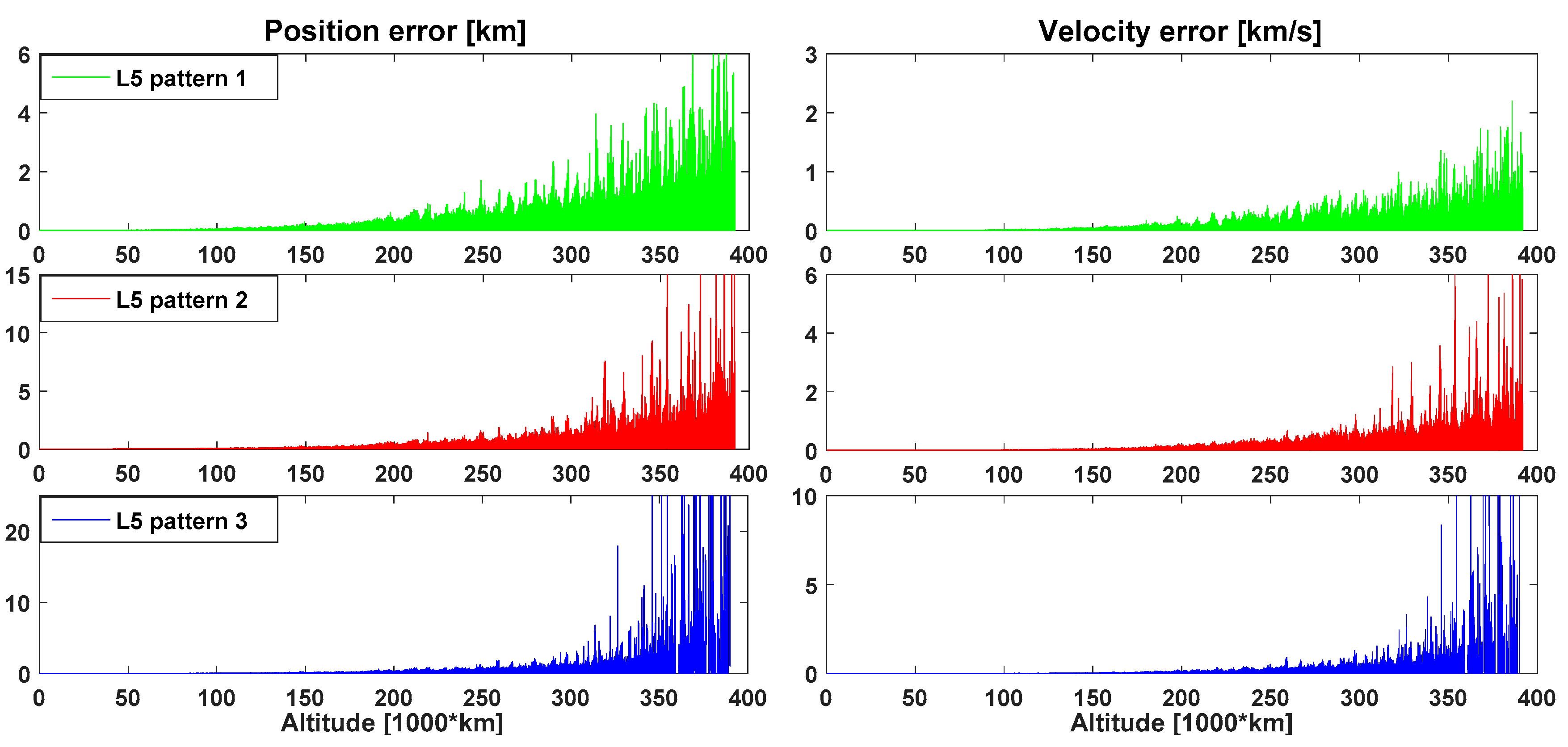
As was done in Section 3.3, Figure 27 and Figure 28 show, respectively, the mean and max for the three considered L5 patterns, assuming 10 dBi receiver antenna gain. We can see that the in case we assume L5 pattern 1 is generally smaller than the other two cases. Indeed, the mean over all trajectory of the mean is 0.57, 0.68, and 0.66 m when assuming L5 pattern 1, L5 pattern 2, and L5 pattern 3, respectively. Moreover, we can see that at the end of the trajectory the in case we assume L5 pattern 3 has a bigger standard deviation in terms of mean and maximal value. As shown, at the end of the trajectory (from 330,000 km until the end), the third L5 pattern results in higher and smaller values of mean .
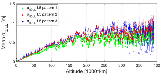
Figure 27.
Mean code tracking thermal noise range error for the assumed MTO. The thermal noise range error is computed for each available PRN and the mean is plotted.
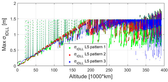
Figure 28.
Max code tracking thermal noise range error for the assumed MTO. The thermal noise range error is computed for each available PRN and the max is plotted.
It is interesting to observe that the maximal up to 325,000 km does not exceed a certain value over time (we can observe a flat area at the top of the plots, which has an approximate value of 1.5 m). This value corresponds to the that the receiver experiences for the minimum that can be tracked (12 dB-Hz for the L5 signal). However, after 325,000 km the maximal reaches higher values. This is the result of the iono-free combination, for which, as shown in Equation (3), the variance is larger than the variance that corresponds to the process of only one frequency (L1 or L5) individually. In our tracking strategy we use a free iono-combination only when the signal is crossing the ionosphere. Signals crossing the ionosphere are also processed in an iono-free combination below 325,000 km, but below this altitude the receiver is also able to process weaker signals from the side lobes, for which the individual is larger.
4.4. Navigation Solution
4.4.1. Least Squares Estimation
Figure 29 shows the zoomed least squares navigation solution for the three assumed L5 patterns. As we can see from this figure, for the entire MTO, when we assume L5 pattern 1 the navigation solution has lower error, while the largest error occurs when we assume L5 pattern 3. Indeed, this was expected as the number of satellites is bigger for L5 pattern 1, leading to better GDOP values. In the case of L5 pattern 3, the relative geometry between the receiver and the transmitters is quite bad, quite often reaching values above 10,000 at the end of trajectory (after 330,000 km), as explained in Section 4.2. Moreover, also the GDOP of L5 pattern 2 has more peaks compared to the one of L5 pattern 1, leading to worse positioning accuracy.
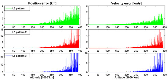
Figure 29.
Single-point least squares estimation error for the assumed MTO.
In Table 7 are shown the quantitative statistics of the navigation solution, for the three defined portions and the full MTO. The statistics for the full MTO confirm what can be seen in Figure 29. However, as shown in Table 7, the statistics for the entire MTO are strongly affected by the third portion, where the navigation performance is much worse for the third defined L5 pattern. Indeed, in the third portion the mean and standard deviation (1σ) of the position error estimation are less than 800 m, less than 1.6 km and several km for L5 pattern 1, L5 pattern 2, and L5 pattern 3, respectively. Also, the maximal error reflects a very big difference; indeed, it is only 6.6 km for the first pattern, more than 22 km for the second one, while for the last pattern it is more than 2000 km. For the first and the second portion, respectively, the difference of the position error estimation is about 0.2 m and less than 20 m among the three assumptions, in terms of mean and standard deviation (1σ). From Table 7 we notice that the velocity error statistics also reflect what was already shown in the position error statistics.
Table 7.
Statistics of the single-point least squares estimation error.
4.4.2. Range-Based Orbital Filter
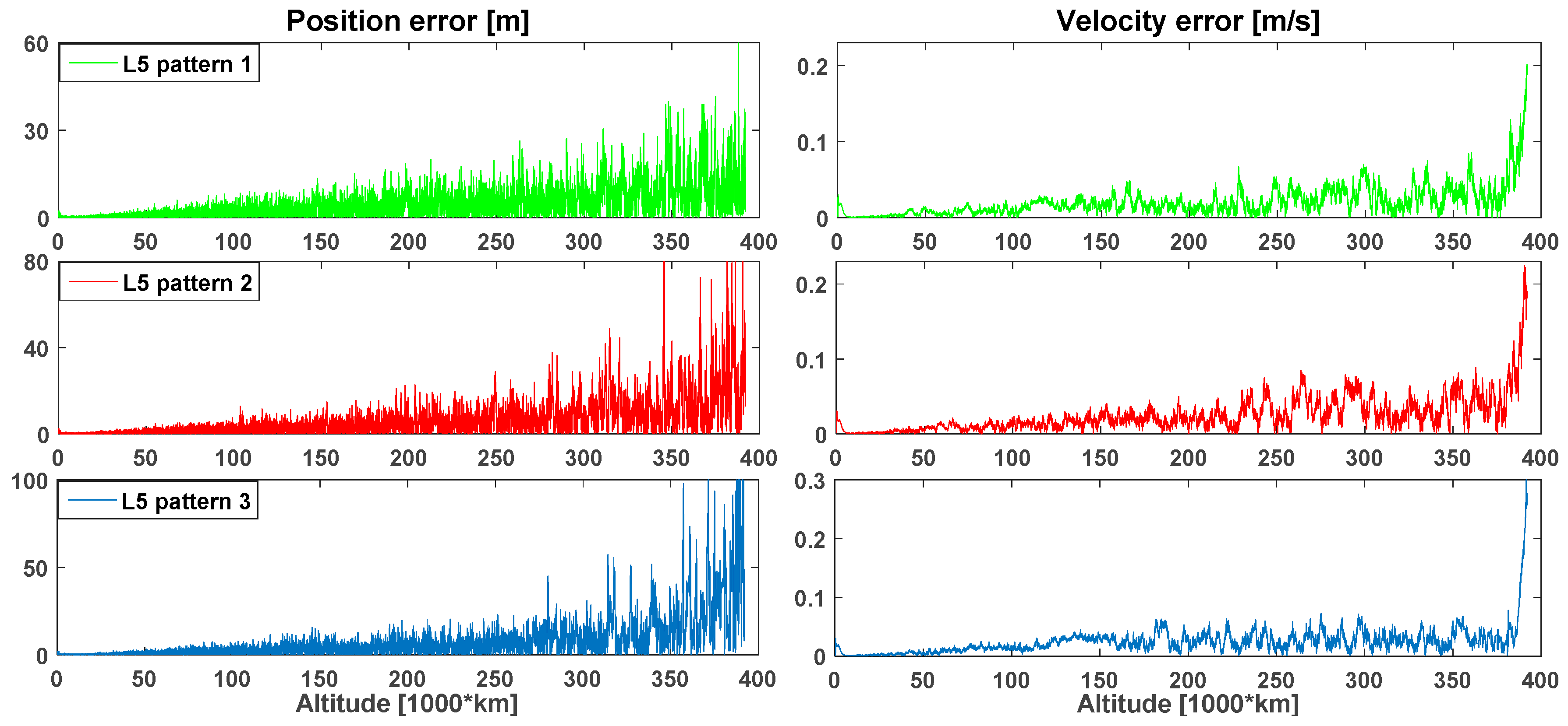
The navigation solution estimation errors, when filtering pseudoranges and pseudorange rates are shown in Figure 30, whilst in Table 8 are displayed the respective statistics for the three defined portions and the entire MTO.
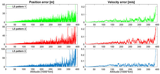
Figure 30.
Range-based orbital filter estimation error for the assumed MTO.
Table 8.
Statistics of the range-based orbital filter estimation error.
Even though the differences of the error statistics are smaller in absolute value, we can still notice that the smaller availability in the case of L5 pattern 3 is reflected in higher error values for the filtered solution in the third assumed portion. Once more, the differences of the position estimation error in the first two portions are very small among the three different assumptions (always less than 1 m in terms of mean and standard deviation), while in the third portion the differences are significant. Indeed, in terms of standard deviation, for the third portion, the errors are approximately 15 times more and 5 times more for the third assumed L5 pattern compared to the first and second assumed L5 patterns, respectively. On the other hand, the velocity statistics are smaller than 0.01 m/s in the first two portions. In the third portion, the difference is smaller than 0.04 m/s in terms of mean and standard deviation and smaller than 0.13 m/s in terms of maximal error. Obviously, filtering the GPS measurements with an orbital filter reduces the impact of the transmitter pattern assumption on the velocity error solution.
5. Number of Available Global Navigation Satellite System (GNSS) Observations for Each Receiver Antenna Elevation
In our previous studies, as well as here, we assumed there was always 10 dB antenna gain at the receiver, which could be provided by one steerable antenna or more than one antenna placed on different faces of the spacecraft (as assumed in [19]). In this section, assuming the L5 pattern 3 (which is the most conservative among the considered antenna patterns defined in Section 2.3), we analyzed the elevations at which the available signals are received by the receiver’s antenna.
It is important to highlight that in our simulations, as illustrated in Figure 31, the spacecraft that hosts the receiver is assumed to be pointing towards Earth, with the same body axis always directed towards the earth’s center. Note that this is not the case in a typical lunar mission; however, for the purpose of this analysis (which only aims at investigating the GNSS signals’ characteristics and the achievable GNSS-based navigation accuracy) it is equivalent to assume that the spacecraft (despite its attitude) will be equipped by one antenna always pointing towards the earth to provide maximum gain. Also note that the elevation is expressed as the semi aperture of a cone, and thus is always positive.
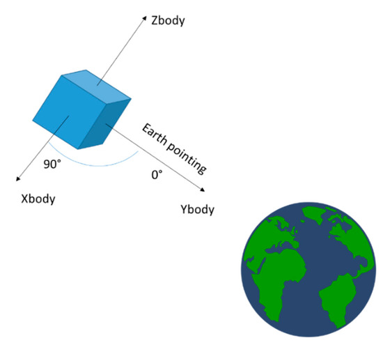
Figure 31.
Earth-pointing attitude configuration assumed for the receiver.
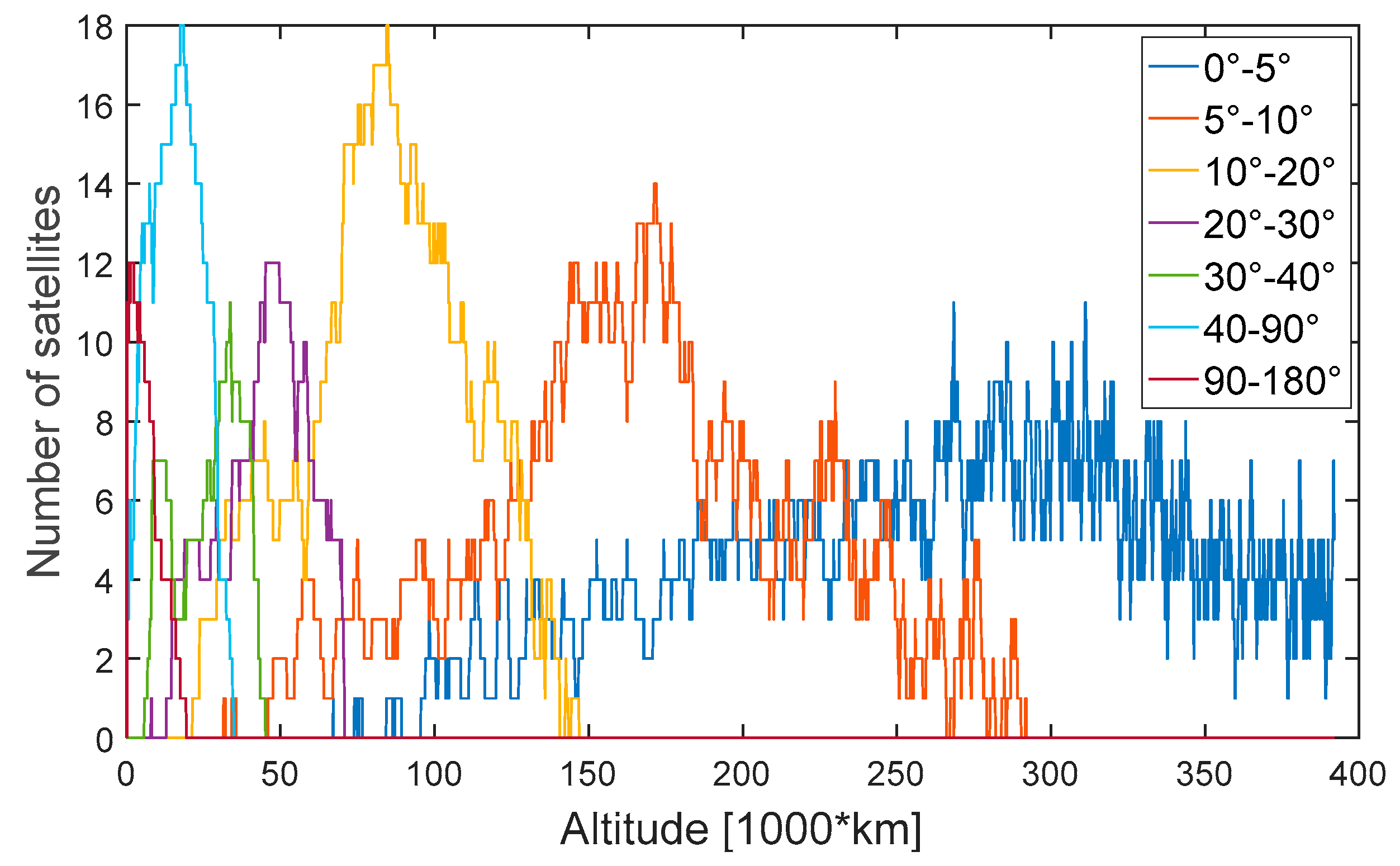
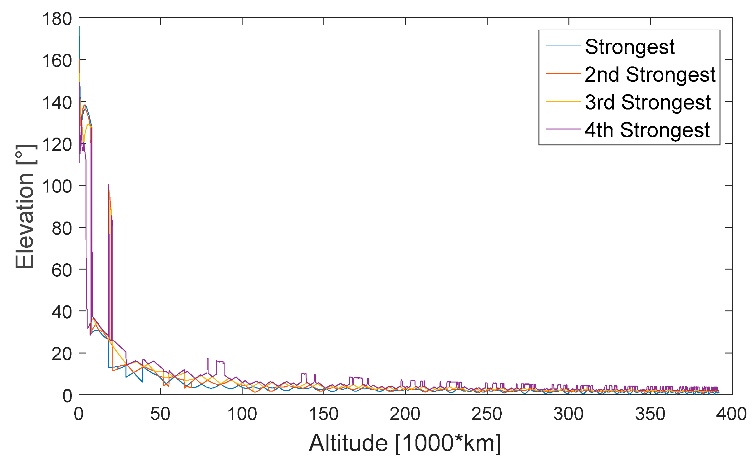
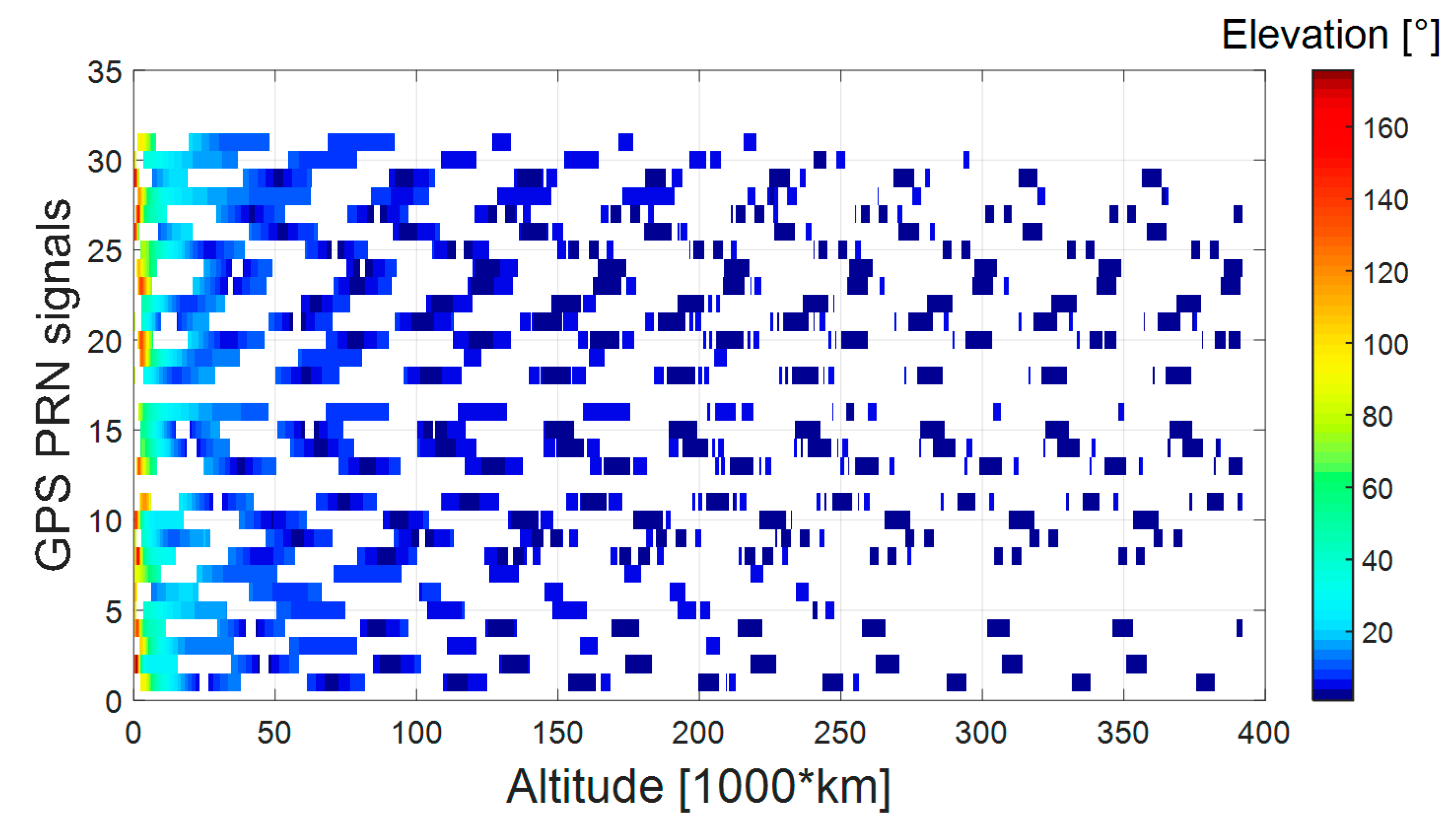
Figure 32 displays the number of available GNSS observations for each receiver’s antenna elevation. Figure 33 displays the elevation values at which the four strongest signals are available at the receiver’s antenna. While Figure 34 shows the PRNs available for each elevation of the receiver’s antenna and for each altitude of the considered trajectory. Figure 35 finally reports a histogram of the available observations for each receiver’s antenna elevation. This information can be useful in order to design an antenna system capable of providing a certain required gain (e.g., 10 dB in our assumptions), at least at the receiver elevations where a minimum of four signals can be processed.
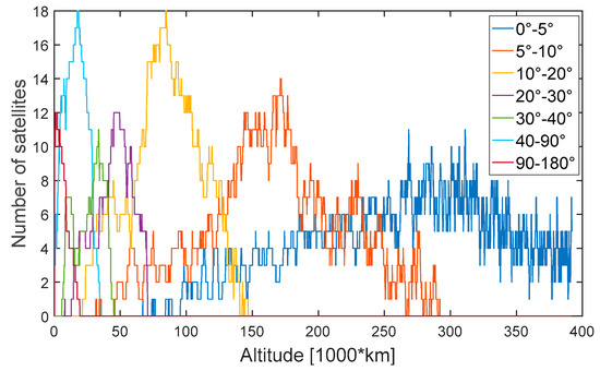
Figure 32.
Number of available global navigation satellite system (GNSS) observations for each receiver antenna elevation for each altitude of the whole considered MTO.

Figure 33.
Elevation values at which the four strongest signals are available at the receiver’s antenna.

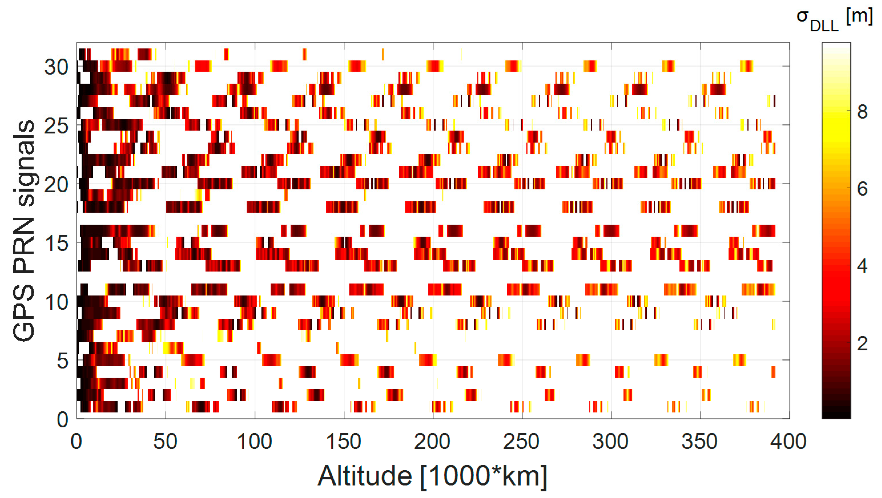
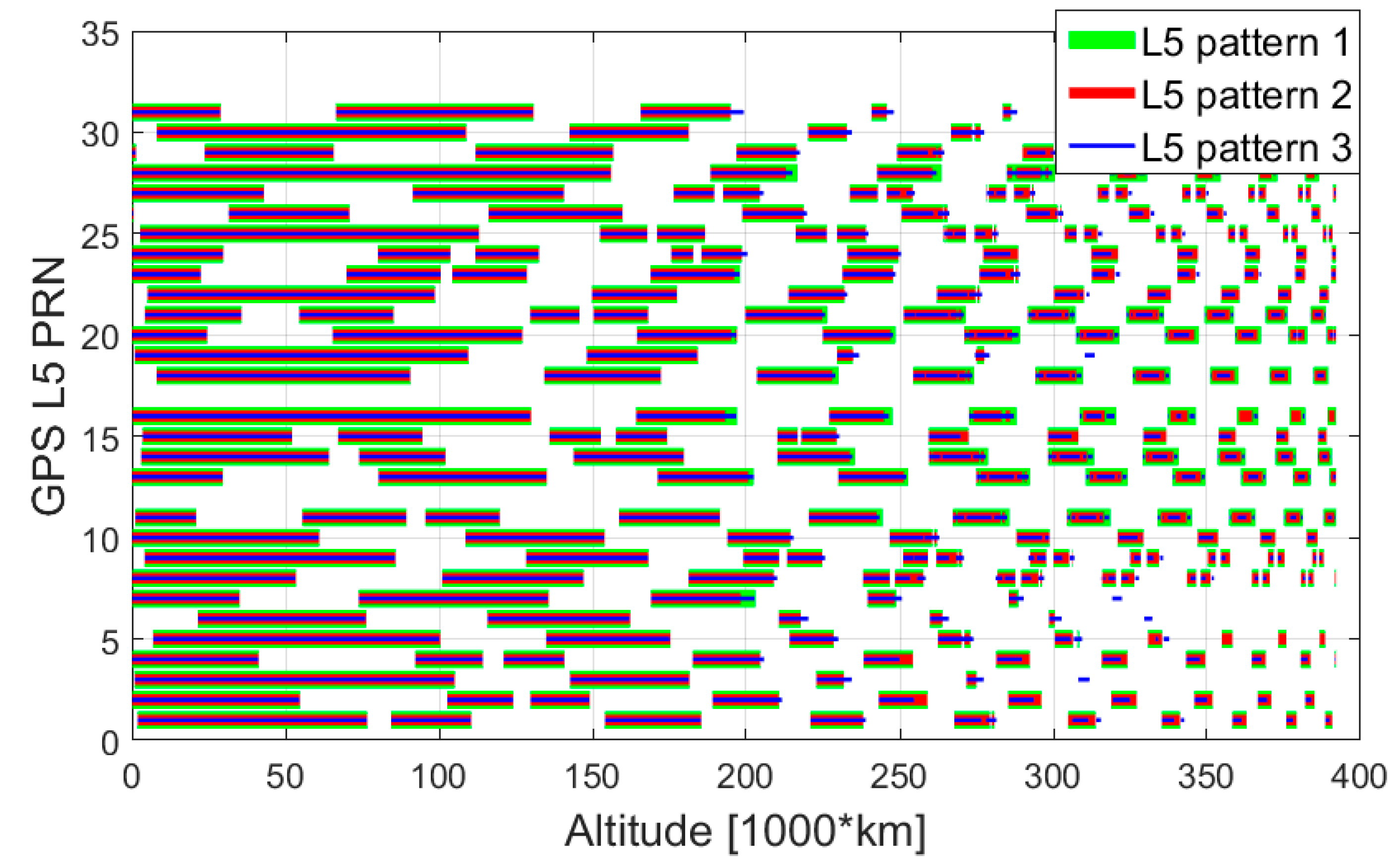
Figure 34.
PRNs available for each receiver’s antenna elevation for each altitude of the whole considered MTO.
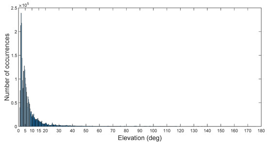
Figure 35.
Histogram of the available observations for each receiver’s antenna elevation during the whole considered MTO.
From Figure 32, we see that above 300,000 km all the signals are received between 0° and 5°, while between 150,000 and approximately 300,000 km there is no available signal at elevations higher than 10°, which means that above 150,000 km a high directivity antenna pointing towards the earth’s center may be sufficient to process most of the signals. From Figure 33, we see that above 100,000 km, the four strongest signals are always received within 10° elevation and at the same time below the same altitude their powers never go below −159 dBm, which is the SANAG receiver sensitivity. Therefore, in principle 10 dB gain from 0° to 10° elevation would already allow the processing of at least four signals. Between the GPS constellation altitude and 150,000 km, most of the signals are received within an elevation interval of 10°–30°; however, as their power is already on average significantly higher than the signals received at higher altitudes (see, for instance, Figure 9), a lower gain for the receiver’s antenna may still allow the tracking of a minimum number of signals. Finally, we see that, as expected, only for altitudes below the GPS constellation are there signals reaching the receiver between 90° and 180°. From Figure 22 and Figure 35 we can observe that, in general, most of the available signals are received between 1.5° and 7°; indeed, most of the mission is spent above 200,000 km, where the spacecraft’s velocity decreases progressively until it reaches the minimum at the apogee.
6. Availability and Angle of Transmission from the Antenna’s Boresight
In this section we analyze the relationship between the availability of a signal at the receiver’s position and the angle from the antenna’s boresight at which the same signal was transmitted. This relationship is of interest since the prediction of the elevation at which the signal is transmitted, as well as the elevation at which the signal is received, combined with the knowledge of the transmitter and receiver antenna patterns, can be used to aid the acquisition process and better attribute the available tracking channels. Indeed, for a receiver with a limited number of tracking channels (i.e., 12 for the SANAG receiver), this information can be used to optimize the attribution of the tracking channels (and thus the channels to acquire as a function of time) in such a way as to only consider the tracking of transmitted signals characterized by a power level at the receiver’s position strong enough to be processed by the receiver (i.e., compatible with the receiver acquisition and/or tracking sensitivity).
In this study, we did not define any PRN selection strategy based on the elevation at the receiver’s antenna, since the definition of the specific spacecraft’s attitude dynamics over time (that depends on the specific mission) as well as of the pattern of the receiver’s antenna(s) placed on the spacecraft would be needed. However, it is possible to predict the elevation at which the signal is transmitted. Then, by assuming a certain transmitters’ antenna pattern, for a certain altitude (and accordingly for a certain free space loss), it is possible to determine the signal’s power at the receiver’s position based on the estimated free space loss, and determine whether the same signal can be processed or not.
Figure 36 displays the histogram of the visible satellites (in the line of sight (LOS)) and of the available satellites (the ones from which the signal transmitted is strong enough to be acquired and tracked by the SANAG receiver) for each transmitter’s antenna elevation during the whole considered MTO. We can see that all the signals transmitted at an elevation angle between 0° and 30° from the transmitter’s boresight are available, i.e., strong enough to be acquired and tracked by the receiver. If the signal is transmitted at an angle above 40° but below 70°, then the chance that it will be available at the receiver’s position will roughly be reduced to 50%. For an angle above 70°, less than 30% of the signals are available.
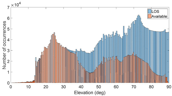
Figure 36.
Histogram of the visible satellites (in the line of sight (LOS)) and of the available satellites (the ones from which the signal transmitted is strong enough to be acquired and tracked be the SANAG receiver) for each transmitter’s antenna elevation during the whole considered MTO.
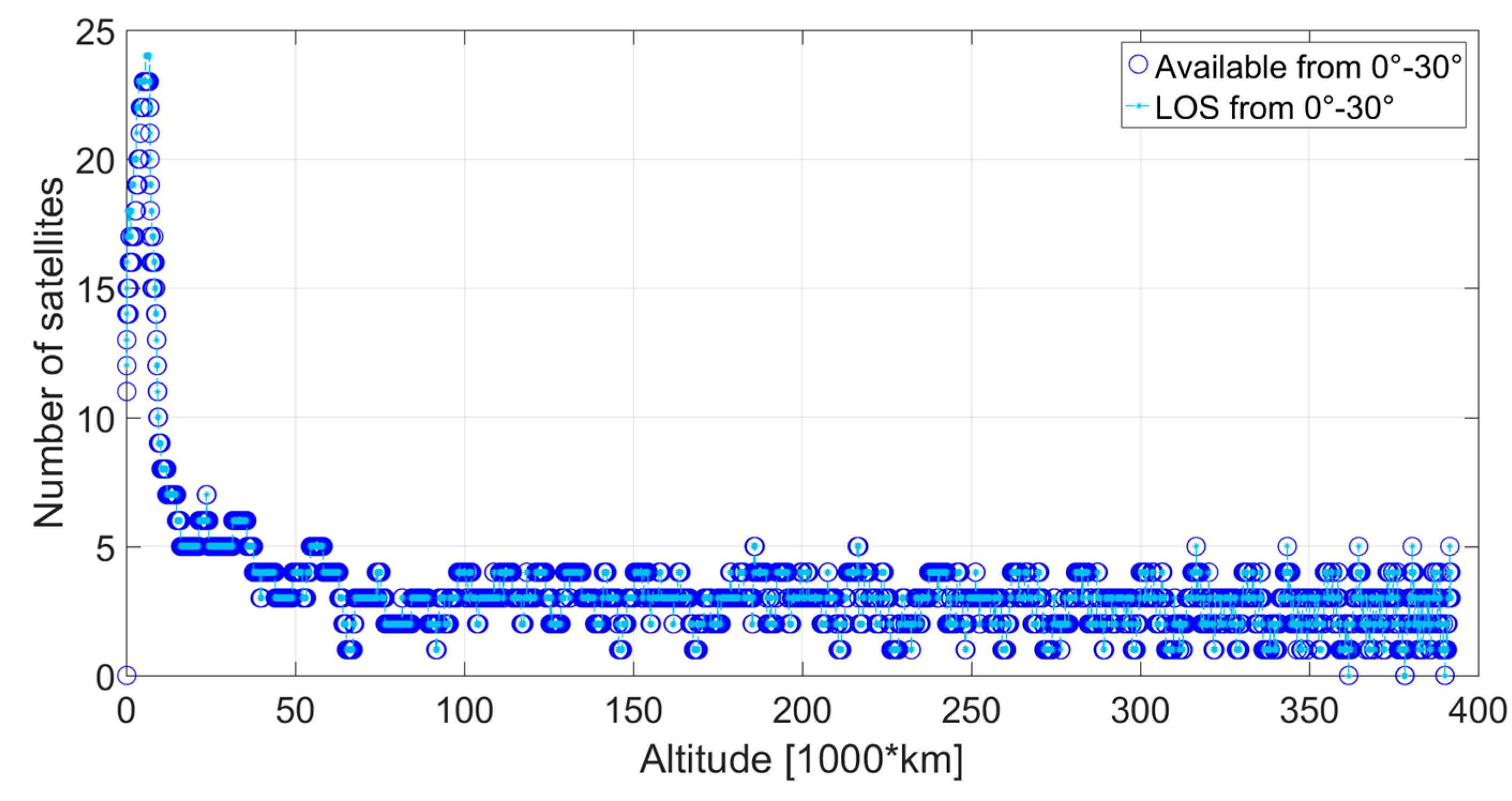
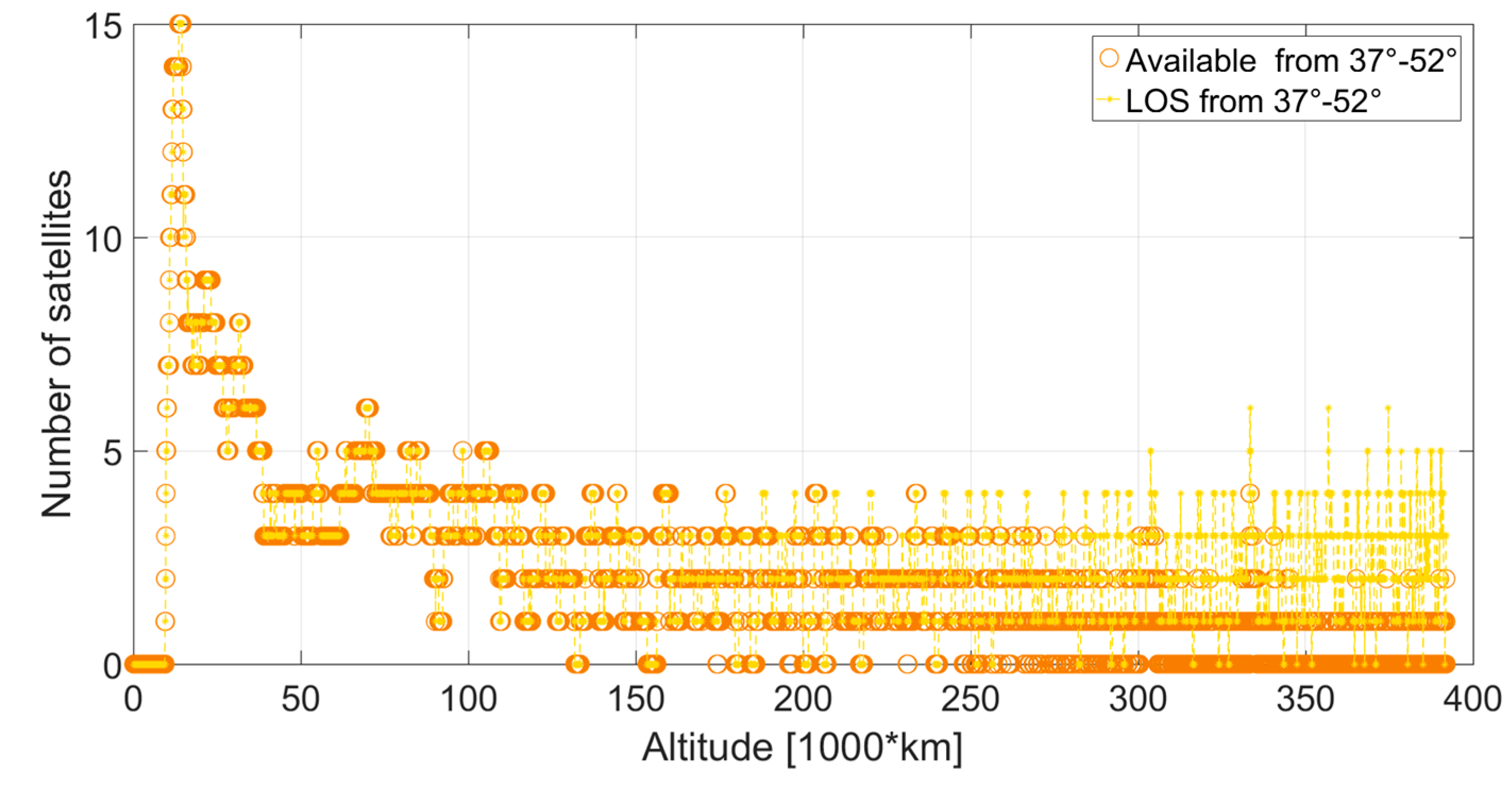
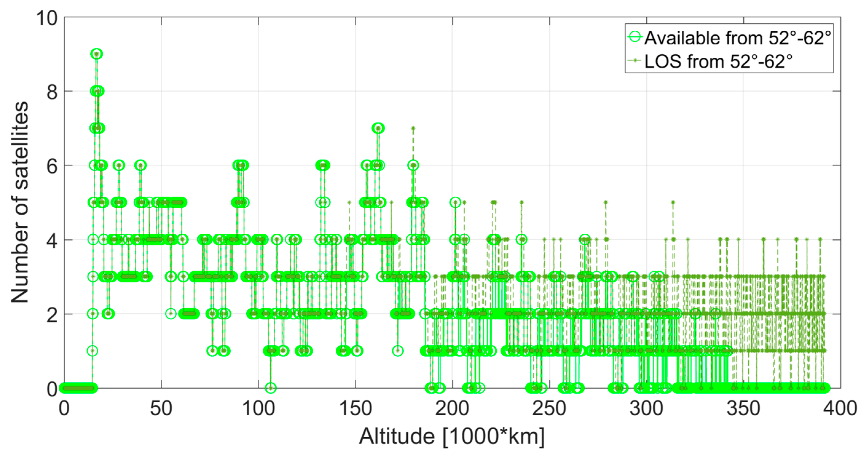
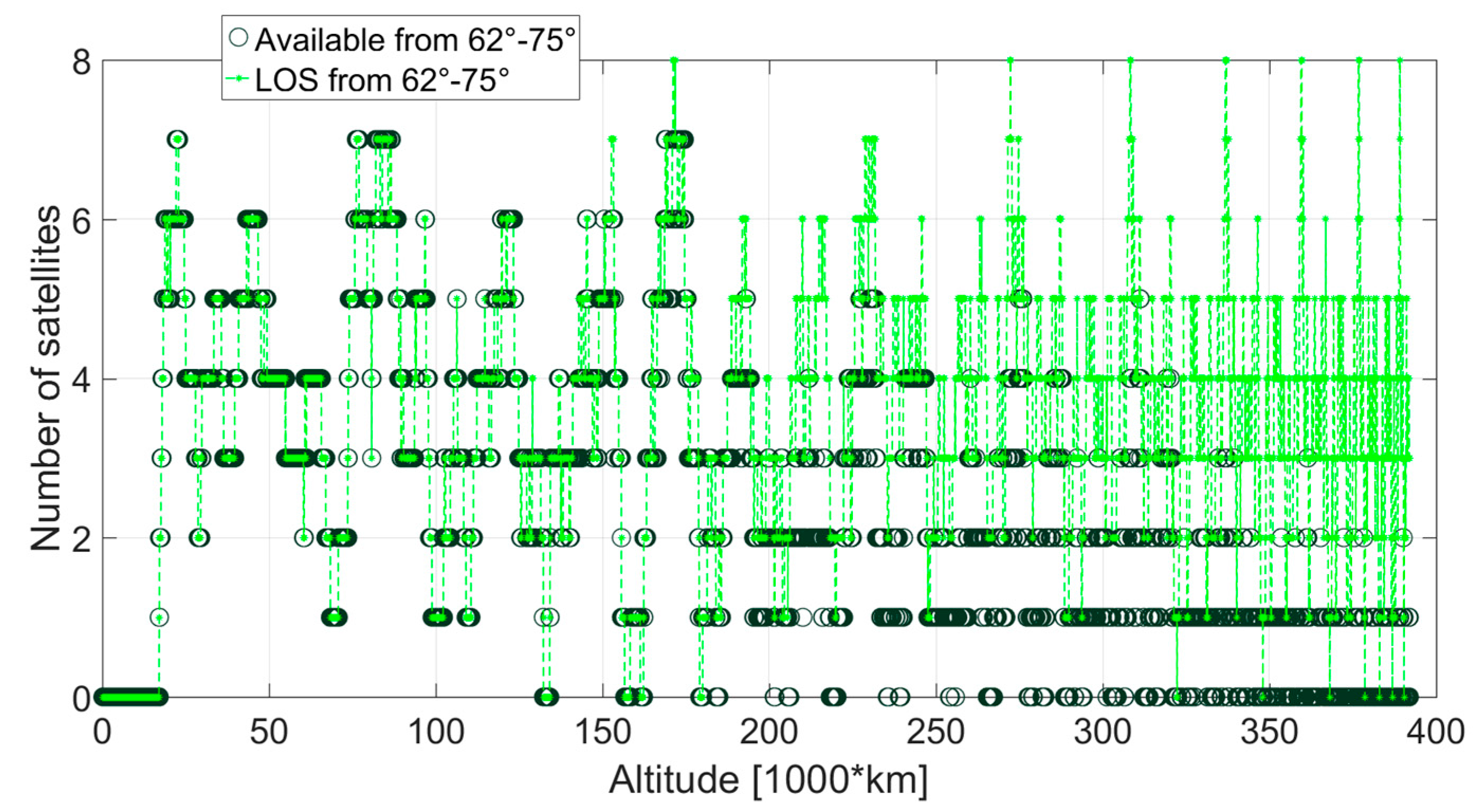
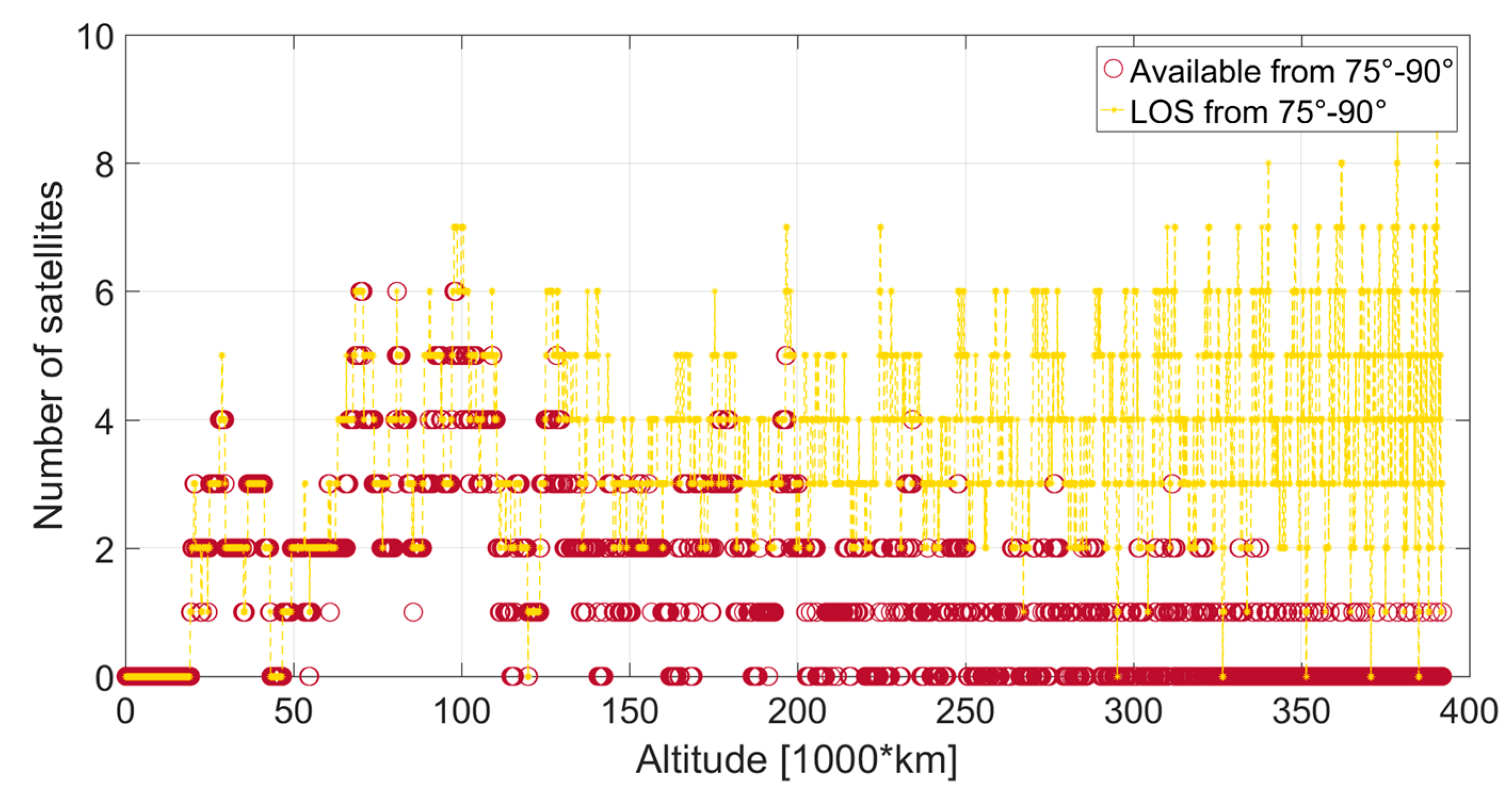
Figure 37, Figure 38, Figure 39, Figure 40, Figure 41 and Figure 42 show the visible satellites (in the line of sight (LOS)) and the available satellites at the receiver’s position, for which the corresponding signal is transmitted at an angle between 0° and 30°, 30° and 37°, 37° and 52°, 52° and 62°, 62°and 75°, and 75° and 90°, respectively, from the transmitter’s boresight. It can be observed that, if the signal is transmitted between 0° and 37°, it is almost always available at the receiver position, from the beginning to the end of the MTO. The signals in the LOS transmitted at angles between 37° and 75° are always available up to approximately 150,000 km of altitude, then available most of the time between 150,000 km and 250,000 km. After that, from 250,000 km to the perigee, a gradual decrease of their availability can be observed. More specifically, only one signal is available out of the four, five, or six transmitted between 37° and 52°. From 340,000 km, none of the signals out of the four transmitted at an angle between 52° and 62° is available. Finally, from 340,000 km, mostly a single signal is available out of the five, six, or seven transmitted at an angle between 62° and 75°. Not all of the signals but most of them transmitted from an angle between 75° and 90° are available up to 130,000 km; gradually fewer and fewer are available up to approximately 340,000 km, and mostly one signal (or sometimes none) is available above 340,000 km. It is interesting to note that above 340,000 km, although mostly not available because too weak, most of the signals are transmitted at an angle between 62° and 90°.

Figure 37.
Visible satellites (in the line of sight (LOS)) and available satellites at the receiver’s position, for which the corresponding signal is transmitted at an angle between 0° and 30° from the transmitter’s boresight.
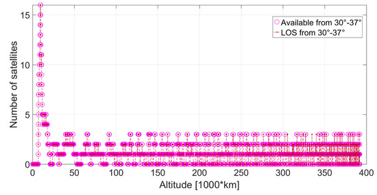
Figure 38.
Visible satellites (in the line of sight (LOS)) and available satellites at the receiver’s position, for which the corresponding signal is transmitted at an angle between 30° and 37° from the transmitter’s boresight.

Figure 39.
Visible satellites (in the line of sight (LOS)) and available satellites at the receiver’s position, for which the corresponding signal is transmitted at an angle between 37° and 52° from the transmitter’s boresight.
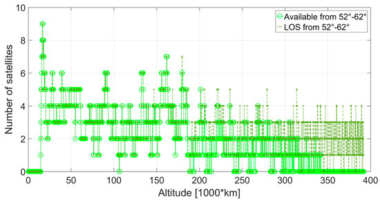
Figure 40.
Visible satellites (in the line of sight (LOS)) and available satellites at the receiver’s position, for which the corresponding signal is transmitted at an angle between 52° and 62° from the transmitter’s boresight.
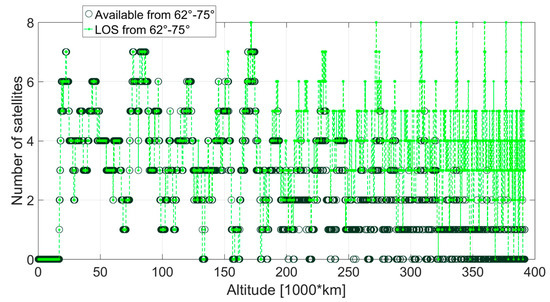
Figure 41.
Visible satellites (in the line of sight (LOS)) and available satellites at the receiver’s position, for which the corresponding signal is transmitted at an angle between 62° and 75° from the transmitter’s boresight.
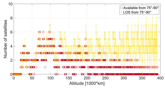
Figure 42.
Visible satellites (in the line of sight (LOS)) and available satellites at the receiver’s position, for which the corresponding signal is transmitted at an angle between 75° and 90° from the transmitter’s boresight.
7. GDOP and Angle of Transmission from the Antenna’s Boresight
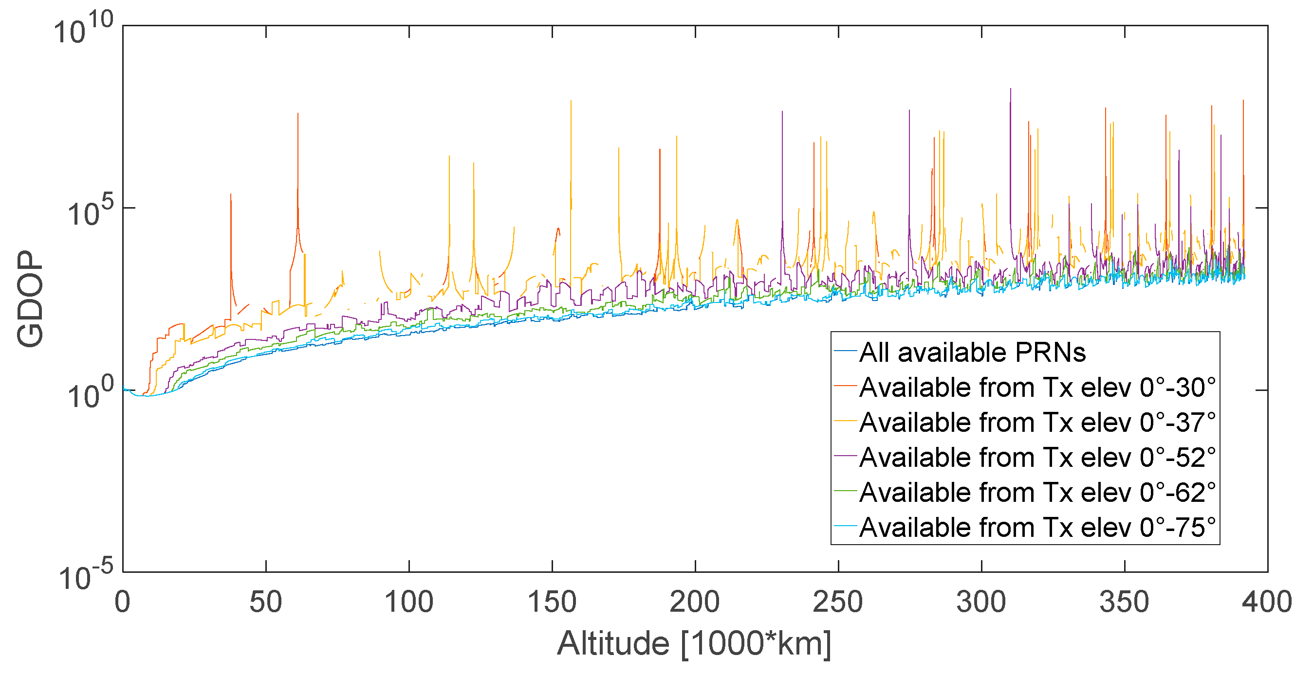
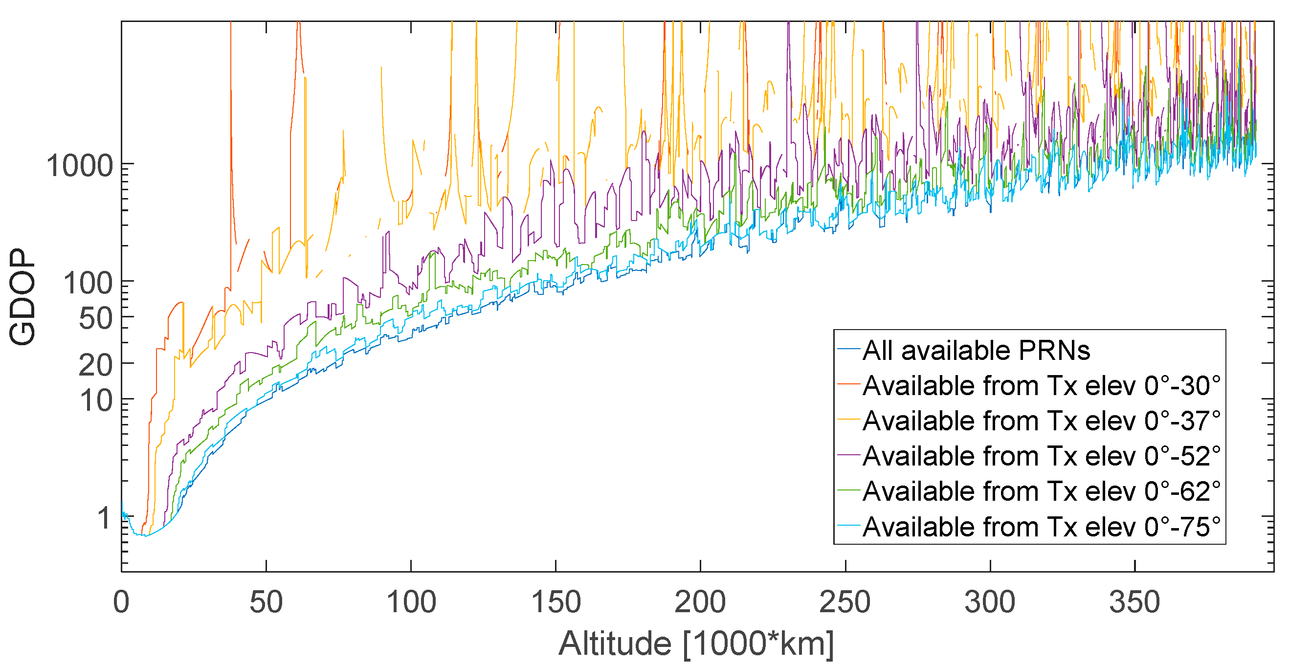
Figure 43 shows the GDOP computed when using all the available signals (each identified by a PRN) and only the ones transmitted at angles between 0° and 30°, 0° and 37°, 0° and 52°, 0° and 62°, 0° and 75°, and 0° and 90°, in order to evaluate what is the relation between the angle at which the signals are transmitted from the GPS satellites and their relative geometry with respect to the receiver. Figure 44 is a zoomed-in view of Figure 43. We can see that if we exclude the signals coming from the side lobes of the transmitters’ antenna (between 30° and 90°), the GDOP worsens drastically: e.g., at 38,000 km from a value of 7 to 83, at 200,000 km from a value of 194 to 1682, at Moon altitude from 1500 to above 30,000. Above 40,000 km, most of the time less than four signals are available (see the orange curve in Figure 43 and Figure 44, which exists only when more than four signals are available) and, when available, the GDOP reaches values dramatically high (above 105). Roughly, we can say that, in order to have at least four signals available at the receiver’s position for the full MTO, the receiver should be able to process signals transmitted at an angle up to 52° from the boresight (the green curve has no discontinuity, while the violet one does, as shown in Figure 43 and Figure 44).

Figure 43.
GDOP computed when using all the available signals (each identified by a PRN) and only the ones transmitted at angle between 0° and 30°, 0° and 37°, 0° and 52°, 0° and 62°, 0° and 75°, and 0° and 90°.
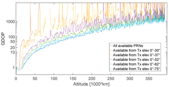
Figure 44.
Zoomed-in view of Figure 43.
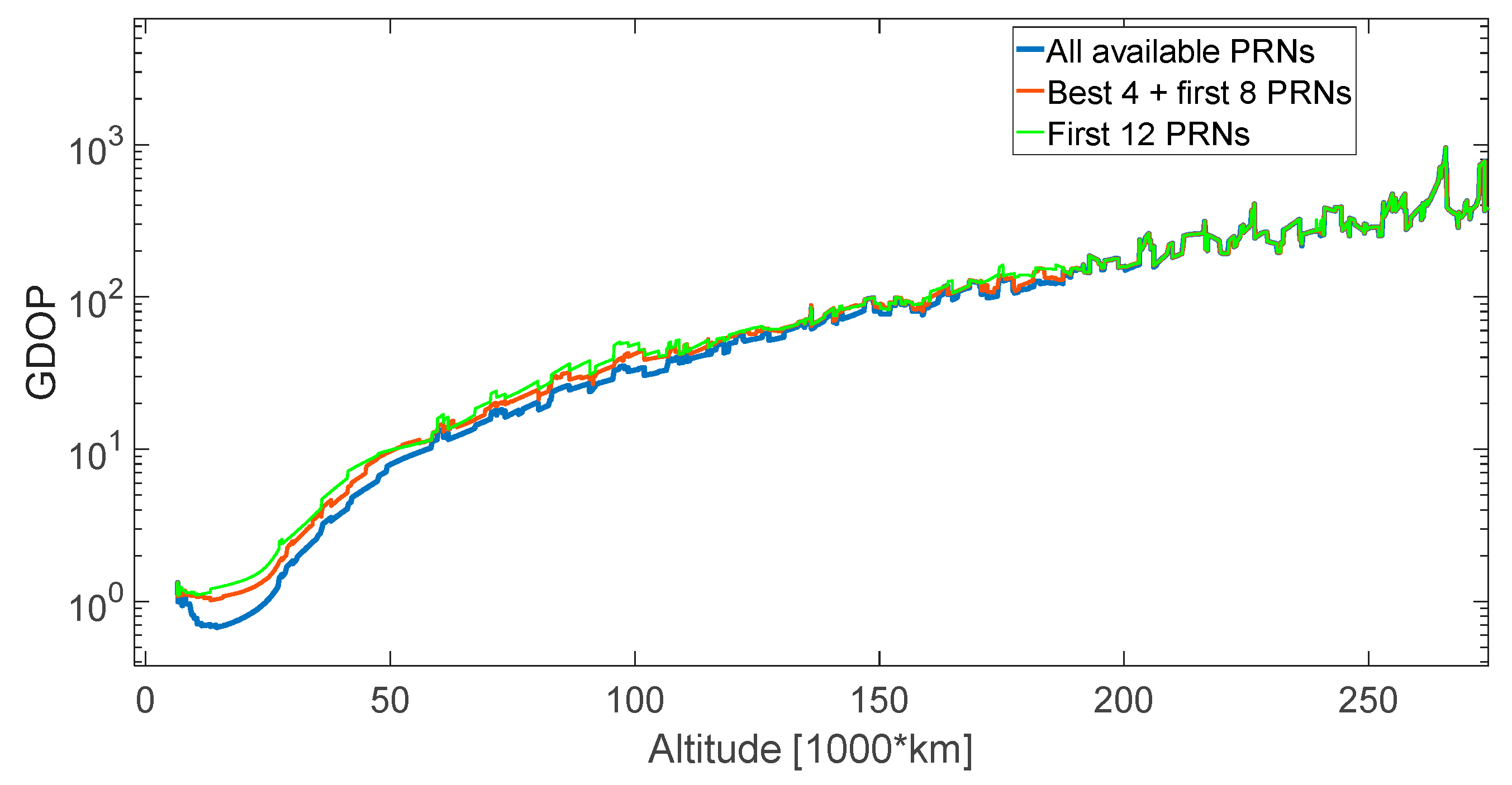
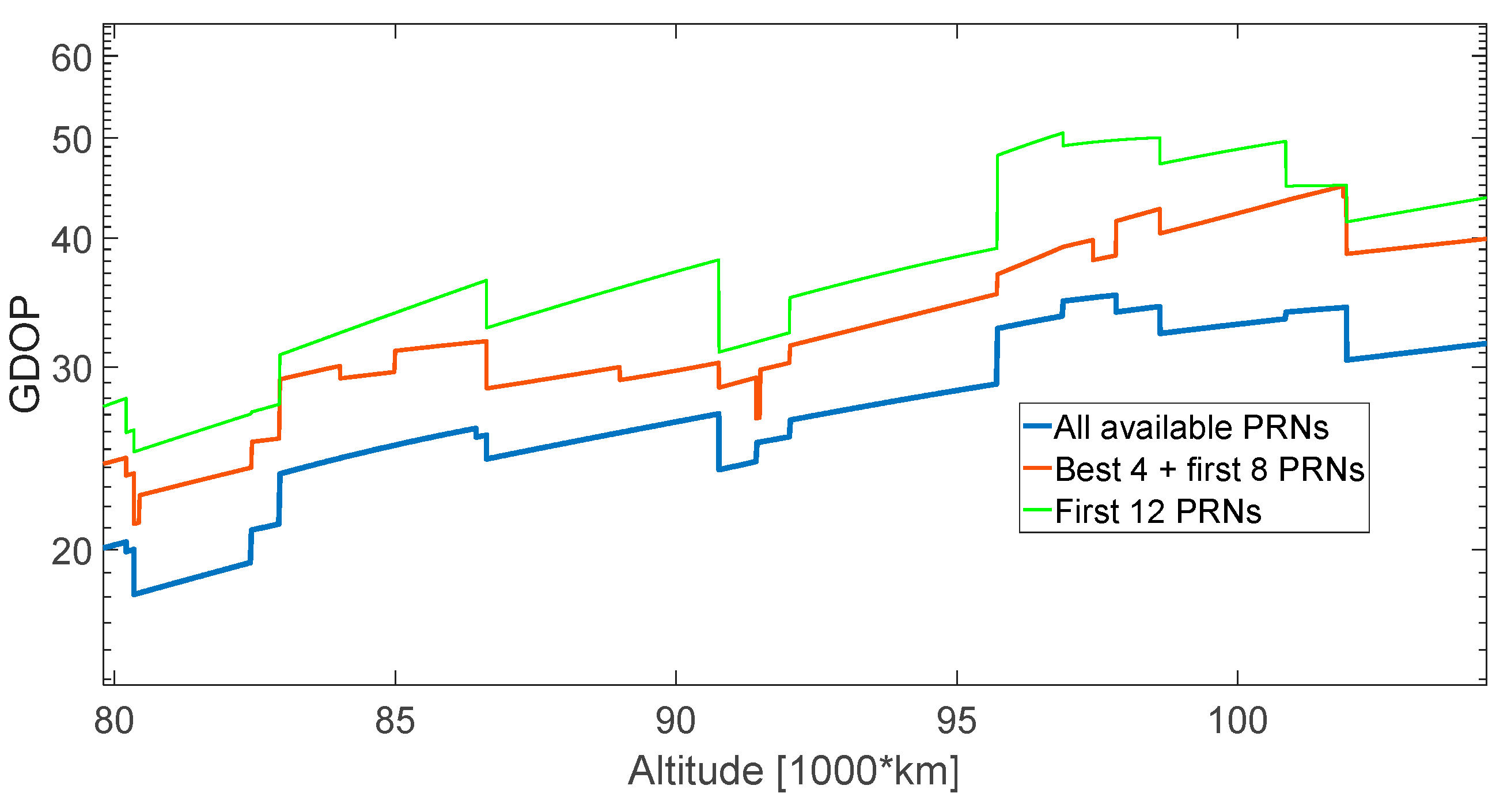
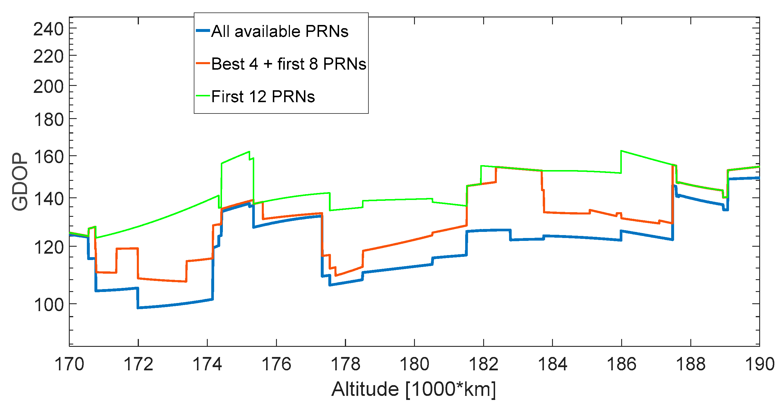
For a limited number of acquisition/tracking channels (i.e., the SANAG receiver should have at least 12 channels), in the lower part of the MTO it is not possible to process all the available signals; for altitudes lower than 187,000 km more than 12 signals are available, as shown in Figure 11. Figure 45 displays the GDOP in three different cases. In the best case, all the available signals are processed (see the blue curve in Figure 45). In the simplest case (see the green curve in Figure 45), the navigation solution is simply computed using the first 12 signals that the receiver processes (e.g., from 1 to 29, the first available PRNs). However, this is not optimal because, among the available signals, there are 12 that ensure the best GDOP. Theoretically, the receiver could predict the combination of 12 signals (among the ones available) that provides the best GDOP, but the associated computational burden may be too high to be performed in real time on board. A less computationally expensive but still effective method is to find the four signals that provide the lowest GDOP and include them in the 12 processed (the brown curve in Figure 45). Figure 46 is a zoomed-in view of Figure 45 between 80,000 km and 105,000 km. For instance, we can see that including the four available signals that give the best GDOP in the 12 processed, instead of just using the first 12 signals that the receiver finds chronologically, provides a GDOP of 35 instead of 48 at 96,000 km (see Figure 46) and of 129 instead of 155 at 187,500 km (see Figure 47).
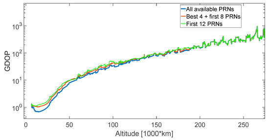
Figure 45.
GDOP in three different cases: when all the available signals are processed (in blue), when only the first 12 signals available are processed (in green, i.e., chronologically the first 12 available from 1 to 29), when the four signals that provide the lowest GDOP are included in the 12 processed (in brown).
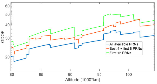
Figure 46.
Zoomed-in version of Figure 45 between 80,000 km and 105,000 km.
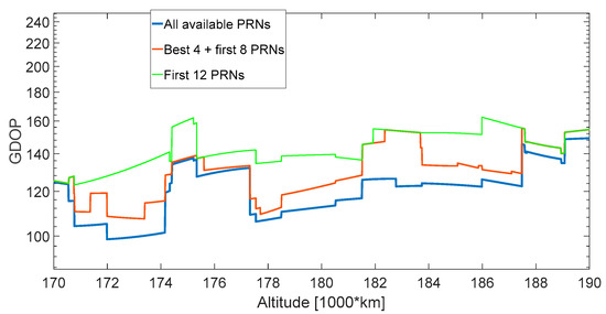
Figure 47.
Zoomed-in version of Figure 45 between 170,000 km and 190,000 km.
8. Conclusions
In this paper, we investigated the effects of different GNSS transmitters’ antenna patterns assumptions on the transmitted signals’ characteristics, in a trajectory that starts from LEO, crossing the SSV and ending at the Moon altitude. In particular, the analysis was carried out by simulating signal power levels, availability, GDOP, code tracking jitter, and, finally, the single-epoch least squares position and velocity solutions, assuming the receiver’s characteristics of the SANAG spaceborne receiver proof-of-concept, under development in our laboratory.
For the transmitters’ antenna patterns of Block IIR and IIR-M L1 we used detailed information, available in the literature, while we were forced to make an assumption (although conservative) on the L1 IIF Block transmitters’ patterns. We analyzed the GPS L1 availability in case the assumed patterns vary as a function of elevation and azimuth (3D pattern) and in case they vary only as a function of the elevation (2D pattern). The results show that the variation in the number of satellites is smaller when a 2D pattern is used. The higher variation in number of available observations when using a pattern changing in both elevation and azimuth causes very big GDOP peaks, which are then reflected in the navigation solution. When the spacecraft is orbiting along the SSV regions only 0.23 satellites per epoch (1 s) on average is the difference in availability (with a maximum of two satellites), while above 200,000 km it is 1.24 satellites per epoch (a maximum of five satellites). Hence, the approximation of the antenna gain pattern does not impact the SSV, but mainly very high altitudes.
We investigated the effect on the SANAG receiver navigation performance for different assumptions on the L5 transmitters’ patterns, for which little information is currently available. From our results we can state that the assumption on the L5 antenna pattern has a small influence on the availability (and consequently on the GDOP) for the two regions of the SSV, where there are always more than seven satellites. However, it is obvious that at very high altitudes, such as the last part of the assumed MTO, the number of available observations is more sensitive to the L5 pattern assumptions; the same happens to the GDOP, which worsens for the third assumed pattern, resulting in a large least-squares solution error. We can conclude that it is important to model the transmitters’ antenna patterns dependency on the azimuth (since using a constant average value is not conservative) and also that for the GPS L5 signal, as expected, assuming a pattern with lower gain values for the side lobes is conservative.
We analyzed the number of available GNSS observations for each receiver antenna elevation during the full mission; 62.8% of the signals are received between 1.5° and 7° from the receiver’s antenna boresight and above 150,000 km only within 10°. Below 150,000 km many signals reach the receiver’s antenna between 10° and 30° elevation, but fortunately with stronger power and without the need for a strong receiver’s antenna gain. Furthermore, we investigated the relationships between the availability and the elevation (the angle from the antenna boresight) at which the signals are transmitted during the full MTO; all the signals transmitted within an angle below 30° from the transmitters’ antenna boresight should be included in the search space for the entire MTO and the ones below 75° should always be included in the search space up to 150,000 km. With the increase in the altitude, the number of available signals transmitted from elevations 30° to 90° is lower and lower than the number of satellites visible in the LOS, making any acquisition aiding strategy harder. Another important result confirmed in this work is that if we exclude the signals coming from side lobes, the GDOP worsens drastically and significantly lowers the navigation performance. Finally, in case we have a limited number of channels (smaller than the signals available), in order to maximize the achievable navigation accuracy, it is important to make a selection among the available signals and use the available channels to process the signals coming from the transmitters that would have the best relative geometry with the receiver.
Acknowledgments
The authors acknowledge the support from the Swiss Space Office of the State Secretariat for Education, Research and innovation of the Swiss Confederation (SERI/SSO), which is financing this research.
Author Contributions
The work presented in this paper was carried out in collaboration between all authors. Cyril Botteron was leading the project and contributed together with Pierre-Andre Farine to the system requirement and implementation definitions, as well as to the overall design discussions. Endrit Shehaj, Vincenzo Capuano and Cyril Botteron conceived the idea of comparing different transmitters’ antenna patterns. Endrit Shehaj and Vincenzo Capuano designed the experiments. Endrit Shehaj performed the experiments, designed and implemented the MATLAB software and performed the simulations. Paul Blunt contributed to the definition of the requirements for the receiver. Cyril Botteron and Paul Blunt contributed to the analysis and the discussion of the results. Endrit Shehaj and Vincenzo Capuano wrote the paper. All of the authors contributed to the revision of the manuscript.
Conflicts of Interest
The authors declare no conflict of interest.
Nomenclature
| ECI | Earth Centered Inertial | MTO | Moon Transfer Orbit |
| GDOP | Geometric Dilution of Precision | POD | Precise Orbit Determination |
| GEO | Geostationary Earth Orbit | PRN | Pseudo Random Noise |
| GNSS | Global Navigation Satellite System | RF | Radio Frequency |
| GPS | Global Positioning System | SANAG | Spaceborne Autonomous NAvigation based on GNSS |
| HEO | High Earth Orbit | SBAS | Satellite Based Augmentation System |
| ICD | Interface Control Document | STK | System Tool Kit |
| LEO | Low Earth Orbit | SSV | Space Service Volume |
| LOS | Line-Of-Sight | UERE | User Equivalent Ranging Error |
| MEO | Medium Earth Orbit | UMT | User Motion Text |
| Received signal power | Line of sight (LOS) unit vector | ||
| Minimum received signal power on Earth | c | Receiver and i-th satellite clock offsets | |
| Global offset | Atmospheric, multipath, signal in space, receiver delays | ||
| Free space loss | Thermal noise code tracking jitter | ||
| , | Transmitter and receiver antenna gain/attenuation | Doppler tracking jitter | |
| Elevation, azimuth | , | Tracking loop parameters | |
| ,, | i-th satellite coordinates | Signal to noise ratio | |
| ,, | Receiver coordinates | Ionospheric-free measurement variance | |
| , | i-th satellite and receiver velocity vectors | L1 and L5 frequencies (, ) square ratio |
References
- Bauer, F.H.; Moreau, M.C.; Dahle-Melsaether, M.E.; Petrofski, W.P.; Stanton, B.J.; Thomason, S.; Harris, G.A.; Sena, R.P.; Parker, L. The GPS Space Service Volume. In Proceedings of the 19th International Technical Meeting of the Satellite Division of The Institute of Navigation (ION GNSS 2006), Fort Worth, TX, USA, 26–29 September 2006; pp. 2503–2514. [Google Scholar]
- Bauer, F.H.; Parker, J.J.K.; Valdez, J.E. GPS Space Service Volume (SSV): Ensuring Consistent Utility across GPS Design. In Proceedings of the 15th PNT Advisory Board Meeting, Annapolis, MD, USA, 11–12 June 2015. [Google Scholar]
- Marquis, W. The GPS Block IIR/IIR-M Antenna Panel Pattern; Loockheed Martin: Bethesda, MD, USA, 2014. [Google Scholar]
- Navstar GPS Space Segment/User Segment Interfaces. 2012. Available online: http://www.gps.gov/technical/icwg/IS-GPS-200H.pdf (accessed on 23 January 2014).
- Mususmeci, L.; Dovis, F.; Silva, J.S.; Silva, P.F.; Lopes, H.D. Design of a High Sensitivity GNSS Receiver for Lunar Missions. Adv. Space Res. 2016, 57, 2285–2313. [Google Scholar] [CrossRef]
- Capuano, V.; Botteron, C.; Wang, Y.; Tian, J.; Leclère, J.; Farine, P.-A. Feasibility Study of GNSS as Navigation System to Reach the Moon. Acta Astronaut. 2015, 116, 186–201. [Google Scholar] [CrossRef]
- Capuano, V.; Basile, F.; Botteron, C.; Farine, P.-A. GNSS Based Orbital Filter for Earth Moon Transfer Orbits. J. Navig. 2016, 69, 745–764. [Google Scholar] [CrossRef]
- Capuano, V.; Blunt, P.; Botteron, C.; Farine, P.-A. Orbital Filter Aiding of a High Sensitivity GPS Receiver for Lunar Missions. In Proceedings of the 2016 International Technical Meeting of the Institute of Navigation, Monterey, CA, USA, 25–28 January 2016; pp. 245–262. [Google Scholar]
- Capuano, V.; Shehaj, E.; Blunt, P.; Botteron, C.; Farine, P.-A. High Accuracy GNSS-Based Navigation in GEO. Acta Astronaut. 2017, 136, 332–341. [Google Scholar]
- Spirent Communications, Spirent GSS8000 Simulator. Available online: http://www.spirentfederal.com/gps/documents/gss8000_datasheet.pdf (accessed on 13 August 2017).
- AGI. STK Astrogator. Available online: http://www.agi.com/resources/help/online/stk/10.1/index.html?page=source%2Fhpop%2Fhpop.htm (accessed on 24 August 2016).
- Blunt, P.; Botteron, C.; Capuano, V.; Ghamari, S.; Rico, M.; Farine, P.A. Ultra-High Sensitivity State-of-the-Art Receiver for Space Applications; Navitec: Noordwijk, The Netherlands, 2016. [Google Scholar]
- Capuano, V. GNSS-Based Navigation for Lunar Missions. Ph.D. Thesis, École Polytechnique Fédérale de Lausanne, Lausanne, Switzerland, 2016. [Google Scholar]
- Navstar GPS Space Segment/User Segment L5 Inter-Faces. 2012. Available online: https://www.navcen.uscg.gov/pdf/gps/IS-GPS-705C.pdf (accessed on 31 January 2013).
- Marquis, W. The GPS Block IIR Antenna Panel Pattern and Its Use On-Orbit. In Proceedings of the 29th International Technical Meeting of The Satellite Division of the Institute of Navigation (ION GNSS+ 2016), Portland, OR, USA, 12–16 September 2016; pp. 2896–2909. [Google Scholar]
- Perello Gisbert, J.V.; Ioannides, R. EIRP Patterns for GPS IIR, IIF Satellite Blocks; ESA MEMO: Noordwijk, The Netherlands, 2013. [Google Scholar]
- Betz, J.W.; Kolodziejski, K.R. Extended Theory of Early-Late Code Tracking for a Bandlimited GPS Receiver. Navigation 2000, 47, 211–226. [Google Scholar] [CrossRef]
- Betz, J.W. Engineering Satellite-Based Navigation and Timing: Global Navigation Satellite Systems, Signals, and Receivers; John Wiley & Sons: Hoboken, NJ, USA, 2016. [Google Scholar]
- Palmerini, G.B.; Sabatini, M.; Perrotta, G. En route to the Moon using GNSS signals. Acta Astronaut. 2009, 64, 467–483. [Google Scholar] [CrossRef]


© 2017 by the authors. Licensee MDPI, Basel, Switzerland. This article is an open access article distributed under the terms and conditions of the Creative Commons Attribution (CC BY) license (http://creativecommons.org/licenses/by/4.0/).