Abstract
This paper presents a novel theory regarding the blade loading and the passage flow field within general turbomachineries. The basic philosophy is to establish an analytical relation between the loading, the flow angle, and the blade geometry based on the conservation of energy. Detailed validations and analyses will be carried out to provide a general scope regarding the theory itself as well as its advantages and limitations in common applications. The paper includes the theoretical derivation of the target relation. The starting point is the standard RANS equations. From that, with the aid of the passage-average operator, the relation between the loading and the passage flow field is derived under the energy balance. Theoretical analyses regarding the validity of the relation are performed based on the simulation results and test data on different cascades. Discussions are conducted regarding the assumption and potential applications of the theory. Conclusions are drawn on the applicability of the theory to introduce its potential applications in general turbomachineries.
1. Introduction
The blade loading, equivalently the flow turning, of a turbomachinery cascade is probably one of the most crucial parameters in turbomachinery design and analysis. Indeed, from the conservation of rothalpy [1], the flow turning through a cascade directly reflects the capability of the work/power generation of a rotating row. As a result, the deviation angle, defined as the difference between the discharge metal angle and the discharge flow angle, has been studied and modeled throughout the past half-century in countless studies. From the perspective of industrial and practical usage, there have been outstanding outcomes from these studies, and they have served well in general turbomachinery designs and analyses. For instance, the famous incidence-deviation correlation developed by Lieblein [2] is an inspiring work for following researchers. Based on the kinematic relation of the in-passage flow quantities, Liebein was able to correlate the data such that the deviation angle is related to the incidence, solidity, and camber. Simultaneously, relating the incidence and deviation to the flow loss via the diffusion factor [3] has later become the most common approach of analyzing blade loading and profile loss in the practical balding designs. Though Lieblein’s work was for early-stage low-speed blades/cascades whose database is too outdated to be utilized for high-speed rows, philosophies within have been adopted by many researchers in the area of blading design/analysis. Cetin et al. [4] established their correlation for transonic compressor cascades. Their correlation modified and extended Lieblein’s model, namely, the incidence and the minimum loss modeling, to the transonic flow regime. Konig et al. [5,6] established the improved deviation and loss model where they extended the diffusion concept of Lieblein’s to the compressible flow regime. Qiu et al. [7] attempted to resolve the generality problem of precedent deviation models by establishing a unified slip factor (equivalently deviation angle) model for axial, radial, and mix-type turbomachineries. From the validation on a vast database of turbomachineries of various kinds, Qiu et al. proved that their model is fairly accurate for various types of turbomachineries compared to precedent models. Other examples of deviation models can be found in various textbooks and articles. These models are particularly useful in meanline analysis [8,9] and rather compatible with the throughflow method [10,11]. As a result, they have been widely used in the phase of preliminary design [12] and optimization of turbomachineries [13].
It is noteworthy, on the other hand, the deviation angle reflects only the net flow turning. In other words, how the loading is distributed along the blade or cascade is not the primary concern of most deviation models. However, the streamwise loading distribution is important in blading designs as it influences the loss characteristics of the blade. Current modeling strategies of loss and deviation are still with the diffusion factor [3], which is based on the assumption that the suction-surface velocity diffusion is the major influential factor of total pressure loss [14]. Such modeling strategies relate the in-passage flow field and the boundary-layer loss empirically or semi-empirically [15], without referring to the physics behind it. Though practically viable, such models and correlations pose problems in terms of accuracy due to advances in blading designs. As a result, most diffusion-factor-based models need to be calibrated with experimental data of up-to-date blade geometries nearly every other decade [16,17]. For instance, recent state-of-the-art fan and compressor rows have compromised almost every assumption made to develop the diffusion-factor-based models: large span size with significant effects of three-dimensionality [18], transonic in-passage flow with shocks, etc. In summary, the in-passage flow, the loading distribution, and the loss must be modeled on a basis that is more physics-oriented.
This paper is the first phase of the research. It aims at investigating the relationship between the loading and in-passage flow field in a quantitative manner. The goal is to develop a novel theory that can quantify the loading or equivalently the local flow turning, with in-passage flow quantities based on the energy balance within the passage. Particularly, following the trace of rothalpy conservation [19], this paper focuses on deriving the energy balance within blade passages and demonstrating the energy propagation pattern introduced by the blade vis-à-vis the flow angle. It is noteworthy that the proposed theory is not of practical use at the moment. Instead, the resultant relations or equations reaffirm some precedent statements on blade loading from a theoretical basis, and these relations and equations can be used for further studies on loading–loss modeling in the future phases of the research.
The mathematical approach used in this paper is the concept of averaging proposed by Adamczyk [20] and Jennions and Stow [21]. Specifically, the moving average operator in the work of Mao and Dang [22] is adopted in this paper for detailed derivations. Using this method, the mean flow quantities, namely, those of interest in practical performance evaluations, are related to in-passage flow characteristics quantitatively. This paper will first introduce the theory that relates blade loading to the in-passage flow quantities. Then, this theory will be examined and validated in different blade rows and cascades. Finally, the conclusion section will discuss the limitation and potential applications of this theory to future work on loss modeling.
2. Theory and Method
In this section, the new theory for analyzing the blade loading and the passage flow field is presented with detailed derivations. For concise demonstration, the governing equations are set for two-dimensional stationary blade passage. It will later be shown that all the presented derivations can be extended to three-dimensional rotating blade rows analogously without losing any generality or mathematical rigor.
For practical usage, standard steady Reynolds Averaged Navier–Stokes simulations suffice in aerodynamic analyses. Therefore, the starting point is the standard two-dimensional Reynolds Averaged Navier–Stokes equation coupled with continuity and energy balance. For two-dimensional stationary blade rows, the flow is approximately steady. Then the governing equations become:
The two-dimensional coordinates are illustrated in Figure 1, where x represents the streamwise direction and y represents the lateral direction.
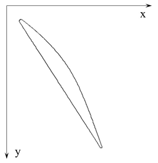
Figure 1.
Concept of a body force model.
For turbomachinery flows, average flow quantities are of more interest since they represent the overall aerodynamic and thermodynamic performances of the row. In that sense, one can see the flow within a blade passage as a simple flow-turning. The average flow for two-dimensional cascades is essentially a one-dimensional flow with lateral velocity (equivalently the swirl velocity for annulus passages). A one-dimensional flow cannot generate a lateral pressure gradient to ensure the momentum balance in the lateral direction, and hence, an extra momentum source is required to exist for this purpose. Indeed, this is the conceptual inspiration of the throughflow modeling, which provides the formulation of such a lateral momentum source, namely the body force.
Though this work does not focus on the throughflow modeling, it can take the advantage of conventional techniques in throughflow to carry on the derivation. Here the method of circumferential average is applied in Equations (1)–(5) to establish the governing equations for the average flow.
2.1. Moving-Averaged Equations
2.1.1. Moving-Average
The moving average operator [23], along with its density-weighted form, is defined, for any arbitrary scalar , as
where is the blade pitch, and is the reference lateral location, indicating the start of the average. The blockage factor is defined as
The gate function , which is to exclude the solid-blade part from the average process, is defined as Equation (8).
In the gate function, is a standard step function, and and are the shapes of the pressure and suction surfaces, respectively (cf. Figure 2). It is noteworthy that the moving average is equivalent to the circumferential average used Jennions and Stow [21].

Figure 2.
Pressure and suction surfaces.
2.1.2. Governing Equations
If one applies these averaging operators in Equations (1)–(5) (examples in Appendix A), the averaged equations can be obtained as Equations (9)–(13).
The term represents the net pressure force acting on the average flow. The term is the perturbation stemmed from the nonlinearity of convective terms. Detailed definitions and formulations of these terms are presented in the Appendix A. Here, only the expressions for body force components are given in Equations (14) and (15) for further derivations.
Note that in common applications, Equations (9)–(13) are used with several important assumptions: (1) the flow within the blade passage is periodic over one pitch; (2) the perturbation terms are negligible due to their relatively small magnitude; (3) the viscous forces, on the other hand, are generally balanced out by the entropy generation based on the boundary-condition property proposed by Denton [24]; and (4) the average stagnation enthalpy is conserved along the mean streamline. Then, the dominant source terms seemingly become the body-force terms. In addition, in order to further guarantee the conservation of stagnation enthalpy, the body force is assumed to be normal to the mean velocity vector, namely
On the other hand, according to the expressions of the two components of the body force, one can have relations as follows
where is defined as
The primed terms in Equation (17) are defined as the difference between the local value of pressure and its average value. Namely
Based on Equations (16) and (17), an interesting relation can be further carried out: the flow angle and the blade mean-camber metal angle σ are related to each other via
If one writes the expression for the body force, then one can have
Equation (21) is an equation of a very neat form. It simply states that the difference between the flow angle and the metal angle (e.g., the deviation angle at the passage exit) depends on the circumferential pressure distribution in the passage, the blade loading, and the thickness distribution. It is noteworthy, however, that Equation (21) does not align with the common observation that a higher loading yields a larger deviation, and it implies singularity at both the leading edge and the trailing edge. This indicates that certain errors must have emerged in the previous derivation; more precisely, the three assumptions proposed before the derivation may be compromised at certain locations and operating conditions.
2.1.3. Errors Related to Neglecting Perturbations
The perturbations are derived from averaging the quadric convective terms. Their expressions, in component form, are as follows:
The double-primed terms in Equation (22) represent the difference between the local value of a quantity and its density-weighted average. Namely,
The physical interpretation of these perturbations is that the non-uniformity of the velocity profile introduces extra flow convections in the average flow field. Mathematically, the magnitude of perturbation depends on two factors: (1) the difference between the velocities on the pressure and suctions surfaces and (2) the shape of the circumferential profile of each velocity component. This indicates that for light-load blades, the velocity difference between the pressure and the suction surfaces are relatively small, and hence, one should expect the perturbation to be also small and vice versa for the high-load blades.
Particularly, for high-load blades, the existence of perturbations compromised the validity of Equation (16), and Equation (21) thereby no longer holds. It indicates that, for high-pressure-ratio compressors, turbine nozzle guide vanes, etc., the error from using equation will be large. In order to account for the influence of perturbations, by enforcing the conservation of stagnation enthalpy, Equation (21) then becomes
2.1.4. Errors Related to Conservations of Stagnation Enthalpy
The conservation of stagnation enthalpy requires a uniform inlet stagnation enthalpy along with the adiabatic condition at solid surfaces. The passage flow meets these requirements, and hence, the average stagnation is conserved through the passage. However, if one investigates the stagnation enthalpy in terms of its definition, one can see how the discrepancy is induced.
The so-called stagnation enthalpy in Equation (12) is defined as
However, the local stagnation enthalpy is defined as
If one applies the average operator in Equation (26), then the average stagnation enthalpy can be obtained as
Clearly, Equations (25) and (27) cannot be simultaneously correct. In fact, precedent researches [22,25] have demonstrated that Equation (12) is strictly true with the definition of Equation (25). However, the conservation of average total enthalpy is a statement for Equation (27). This entails that applying the conservation of total enthalpy for Equation (12) is not rigorous since the perturbations in Equation (27) are overlooked. Hence, errors will be introduced into Equation (24). In order to compensate such a discrepancy, one must add the perturbations into the derivation and that results in Equation (28) (assuming the condition proposed by Denton [24] that the viscous dissipation is completely drained by the heat transfer):
where is defined as
Since the mean stagnation enthalpy is conserved given that it is uniform at the inlet, then Equation (24) can be further modified to
From Equation (30), one can see that the average flow deviation is influenced by three factors: (1) the thickness distribution coupled with the loading condition, (2) the work done by the perturbations, and (3) the nonlinearity of the stagnation enthalpy. According to the definitions of each term, one can further state that the flow deviation can be quantified using the blade geometry and flow-field information. For future reference, the three factors are referred to as pressure-thickness (P-T) effect, perturbation (Perturb) effect, and perturbed stagnations enthalpy (PSE) effect, respectively.
2.2. Extension to Moving or Rotating Blade Rows
Note that Equation (30) is derived for two-dimensional stationary planar cascades. Similar equations for three-dimensional moving/rotating planar or annulus cascades can be derived analogously. The only differences are that for three-dimensional flows, the flow angle is defined based on meridional velocity, which represents the radial and circumferential shifting of the mean streamline (cf. Figure 3); and for rotating or moving cascades, the stagnation enthalpy is replaced with the rothalpy. For coordinates defined in Figure 3, the following are different versions of Equation (30) for different types of blade rows:
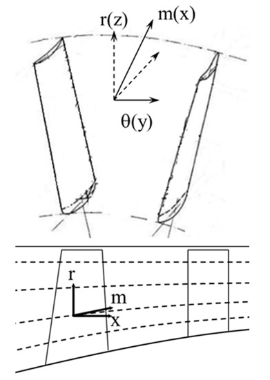
Figure 3.
Coordinates system for 3-D (2-D) flow.
For three-dimensional moving planar cascades, the expression becomes
For three-dimensional stationary annulus cascades, the expression is
For three-dimensional rotating annulus cascades, the expression is
In the following sections, Equations (30)–(33) will be validated for different types of cascades using RANS simulations. Particularly, each term in these equations will be evaluated thoroughly to demonstrate the important flow physics related to passage flow.
3. Validation and Analysis
This section focuses on the validations and analyses of Equations (30)–(33). It is noteworthy that prior derivations are not bound to any specific types of cascades or blade rows nor are they to any specific operating conditions. Hence, one should expect these equations to be valid in a general sense. To the authors’ interest, on the other hand, the validity of the theory in different flow regimes is of significant importance. Therefore, validations are to be performed based on the variation of flow regime, coupled with cascades or blade rows of different types under multiple conditions.
All the following CFD simulations are performed with ANSYS Fluent. The solver is its embedded steady RANS solver with the standard k-epsilon model. The algorithm is the SIMPLE algorithm. All the discretization schemes are 2nd order accurate. The convergence is met when the relative error reduces by five orders of magnitude. Other details regarding this solver can be found in [26].
3.1. Low-Speed Cascades Validations
3.1.1. Cascade Geometry and Case Setup
The moving average operator, along with its density-weighted form, is defined, for any arbitrary scalar
The compressor cascade selected is the NACA 65-4-10 compressor cascade [27] because of the vast amount of available data. The geometry of the cascade is shown in Figure 4. Some important aerodynamic specifications of the cascade are listed in Table 1.

Figure 4.
NACA 65-4-10 cascade.

Table 1.
Geometrical and aerodynamic specification of NACA 65-4-10.
The turbine cascade selected is the NASA LPT guide vane cascade [28]. It is a light-load guide vane with mild thickness variations (cf. Figure 5). Relevant aerodynamic specifications of this cascade are listed in Table 2.
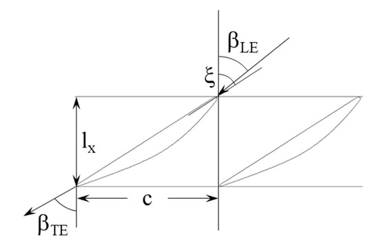
Figure 5.
NASA LPT cascade.
Table 2.
Geometrical and aerodynamic specification of NASA LPT cascade.
Since both cascades are 2D planar cascades, the computational domain is similar for both simulations. Taking the NACA 65-4-10 cascade simulation as an example, the computational domain and mesh are shown in Figure 6. Mesh qualities are listed in Table 3. The boundary conditions are demonstrated in Figure 7.
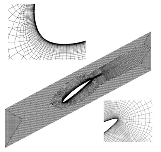
Figure 6.
Mesh for NACA 65-4-10 cascade.
Table 3.
Mesh quality for NACA 65-4-10 calculations.

Figure 7.
Boundary conditions for CFD simulations.
3.1.2. Results and Discussions
First of all, for the mesh dependency study, four meshes are used to perform the simulation. The results from the finest mesh of 400,000 cells are taken as the reference case. The relative error of discharge flow angle is defined as Equation (34).
The relative error versus mesh size for the NASA 65-4-10 case is plotted in Figure 8. The cascade friction coefficient converges with the mesh size at the logarithmic slope of -1.65. This indicates that the CFD simulation results are in good fidelity, and it is justified that these results are being used for further analyses.
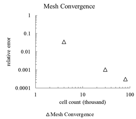
Figure 8.
Mesh dependency study.
Note that if the mesh topology for the NASA LPT guide vane cases is similar, the conclusion regarding the previous mesh convergence study can be postulated to these cases as well.
The first step is to examine the accuracy of the CFD simulations. The CFD results are compared with the experimental data in terms of the discharge flow angle and the pressure distribution on the blade surface for the NACA 65 cascade and the NASA LPT cascade, respectively. The comparison is illustrated in Figure 9 and Figure 10, respectively. Figure 9 demonstrates good agreements until the AoA of 17 degrees. This is because at about AoA of 17 degrees, massive separation occurs in the passage, and thus, the steady RANS simulation will lose accuracy inevitably. Figure 10 showed a very good agreement between the CFD results and test data. In all, CFD simulations predicted key aerodynamic characteristics quite accurately in most operating conditions, and hence, the CFD predicted in-passage flow can be used to reflect the physical in-passage flow field.
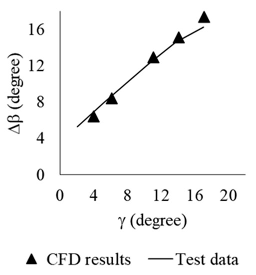
Figure 9.
Validation of NACA 65-4-10 cascade simulations: Discharge flow angle vs AoA.
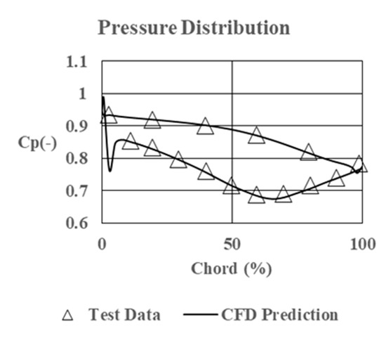
Figure 10.
Validation of NASA LPT cascade simulations: blade–surface pressure distribution.
The next step is to evaluate the magnitude of each term in Equation (30), using the flow-field quantities extracted from the CFD results. Figure 11 demonstrates the comparison between the actual flow angle and estimated flow angle using Equation (30). The dashed line represents the outcome of the RANS simulation, and the symbols are the flow angle predicted by the theory. The solid triangle represents the P-T effect; the solid square represents the perturbation effect, and the solid circle represents the contribution of PSE. The blank triangles represent the compound effect of the former three component effects. From Figure 11, one can conclude the model is very accurate provided that the dashed line and the blank triangles are spot-on matches. Beyond that, it is also observed that the P-T effect alone is fairly close to the compound effect. This is consistent with the precedent statement that perturbations and PSE effects are not influential on the flow inside light-load cascades [29].

Figure 11.
Model validation results (NACA 65).
For the turbine cascade, Figure 12 demonstrates the comparison between the actual flow angle and the estimated flow angle using Equation (30) at different streamwise locations. The trend shown in Figure 12 is consistent with that in Figure 11 as both cascades are of light load. The P-T effect in Equation (30) alone is very close to the dashed line that represents the compound effect except at the trailing edge. This is, however, expected. The size of the trailing edge of a turbine cascade is comparable to the length scale of the cascade itself. Therefore, the nearby flow field is influenced by the presence of the trailing edge. More specifically, the pressure and velocity are more circumferentially distorted due to the effect of the larger trailing-edge blunt body, rendering a heavier perturbation effect, compared to that in a compressor cascade, where the size of the trailing edge circle is marginal compared to the size of the cascade.

Figure 12.
Model validation results (NASA LPT).
In all, one can conclude that for light-load cascades, Equations (21) and (30) both show high accuracy. In particular, Equation (21) shows a direct relation between the thickness variation of the blade and the flow angle. Such a simple relation can be very useful in practice. In the inverse design of a light-load blade, for instance, if the pressure loading is prescribed as design input, then the thickness of the cascade can be easily determined.
3.2. High-Load Subsonic Cascade Validations
In order to evaluate the effect of higher loading, a high-load turbine guide vane cascade is used to perform validations. It is to investigate to what extent the loading interacts with the in-passage flow field and thus the perturbations and perturbed stagnation enthalpy.
3.2.1. Cascade Geometry and Case Setup
The NASA E3 turbine guide vane [30] is selected since it operates in the high subsonic regime (Ma = 0.8) with very aggressive flow turning. The geometry and aerodynamic specifications of this cascade are included in Figure 13 and Table 4, respectively.

Figure 13.
NASA E3 guide vane cascade.
Table 4.
Geometrical and aerodynamic specification of NASA E3 cascade.
The computational domain and mesh topology of this set of calculations are similar to previous simulations. The mesh dependency study for this case is therefore skipped. The mesh quality is demonstrated in Table 5.
Table 5.
Mesh quality for NASA E3 cascade.
3.2.2. Results and Discussions
First of all, the CFD simulation results are compared against the test data. The quantity of interest is the pressure distribution on the blade surface. The comparison is shown in Figure 14, and CFD simulations predict the pressure distribution rather accurately. This justifies further analyses using these CFD results.
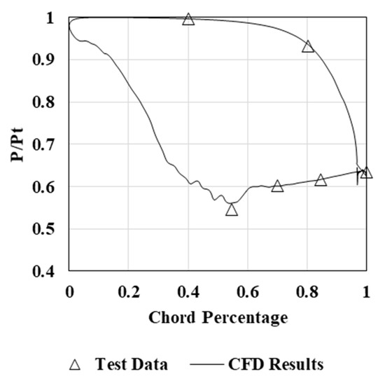
Figure 14.
Blade-surface pressure distribution of NASA E3 cascade.
From the CFD results, the circumferential distributions of velocity and pressure are extracted. As shown in Figure 15, these profiles become highly distorted inside the passage. Such distortions come from two sources: (1) the convergence and divergence of the passage and (2) the very aggressive metal angle. This is consistent with the intuitive understanding that the higher the loading, the more distorted the circumferential profile will be. Moreover, it can be observed that profiles at the LE and the TE are both quite uniform compared to those in-passage profiles. This indicates that for the given cascade, the variation of the profile shape may follow a certain pattern, that is, uniform to distorted and then to uniform, from the LE to the TE. This may be useful if one were to evaluate the flow field at off-design conditions with the aid of scaling analysis.
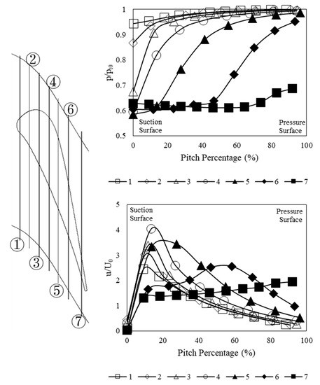
Figure 15.
Quantity distributions at different axial locations: (up) static pressure distribution; (down) axial velocity distribution.
Validation results are illustrated in Figure 16. From the results, one can see that the model prediction is very sensitive to the magnitude of each effect at the LE. Such sensitivity decreases towards the TE. This is the case for this cascade since it is a high-turning cascade, and the metal angle is large compared to the flow deviation. It implies that the pressure and velocity distortions induced by the blade interact with the inflow and thus greatly influence the local flow turning. Indeed, the LE flow has long been a problem of tremendous complexity. Focusing on either the velocity field or the pressure field alone will not suffice for resolving the flow turning in this region.

Figure 16.
Model validation results (NASA E3).
Within the passage, unlike those for the light-load cascade where the P-T effect can be qualitatively representative of the flow angle, the three effects in the high-load cascade are more interactive with each other, rendering the flow angle a consequence of the compound of these three component effects.
As for the TE, if one enlarges the scope in the circled area in Figure 16, one can see that the actual flow angle coincides with the flow angle predicted by the perturbation effect alone (cf. Figure 17). This implies that towards the TE, the flow turning becomes eventually perturbation dominant rather than almost equally influenced by all the three effects. This observation is different from those in light-load cascades, and they can be rather useful in practice as they may provide potential approaches for estimating the deviation angle for such high-load cascades. For instance, together with the wake theory [31], one can estimate the circumferential profiles of velocity components and evaluate the perturbations and therefore the discharge deviation angle or flow angle.

Figure 17.
Model validation near the TE.
Another important observation is that the P-T effect shows different influences upon the flow turning at location 6 and location 7. This is because locations 6 and 7 are on both sides of the passage exit, as shown in Figure 15, and hence, the pressure field pattern is different at these two locations. This observation indicates that the flow deviation near the TE is a quantity of strong local effect. Indeed, for a high subsonic turbine guide vane, the trailing edge flow contains very complex shock systems that can hardly be described by a general analytical formulation.
3.3. Transonic Fan Rotor Validations
Another influential factor worth investigating is the shock wave. Some researchers have demonstrated that the precondition (12) is not well-defined in the presence of an axisymmetric shock [32], rendering Equation (20) invalid on such occasions. However, the energy balance should not be influenced by the existence of shocks. Hence, one should expect consistent validities of Equations (30)–(33) for transonic cascades. Nevertheless, the statement is rigorous only if these equations are validated in a transonic blade row, and the NASA ADP Fan [33] (cf. Figure 18)) is then selected for such validations.
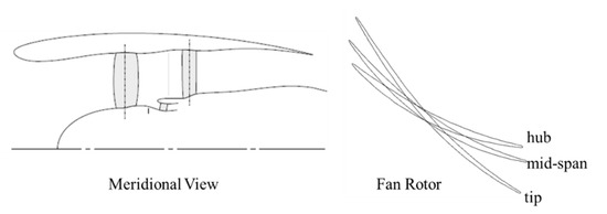
Figure 18.
NASA ADP fan geometry.
This is a transonic blade of strong three-dimensional characteristics and simultaneously a rotating blade row. Accordingly, Equation (33) is used in the following validations. If the following validations show good agreements between the theory and the physical flow field, they indicate that the proposed theory is valid for not only stationary planar cascades but also moving annulus cascades.
3.3.1. Cascade Geometry and Case Setup
The geometry of the blade is shown in Figure 18. The CFD simulation is carried out to replicate that of Tweedt [34]. The nacelle and nozzle are also included in the computational domain. The operating conditions of interest are Sea Level Take-Off (SLTO), Cutback, and Approach. The boundary conditions of the simulation are also illustrated in Figure 19. The rotor and stator interfaces are modeled using the mixing plane method [35].
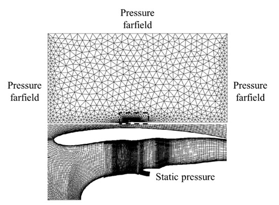
Figure 19.
Computational domain of NASA ADP fan simulation.
3.3.2. Results and Discussions
First of all, the CFD results are validated against the test data. From Figure 20, it is demonstrated that the CFD simulation replicates the test data very accurately. It justifies that the CFD simulation results reflect the physical flow field in this fan system.

Figure 20.
NASA ADP fan CFD validations: total temperature and total pressure profiles upstream of OGV.
The next step is to evaluate the magnitude of each term in Equation (33). The step is performed at the SLTO operating condition, at 89% span from the hub to ensure that there is a transonic flow region in the passage. The results are shown in Figure 21.
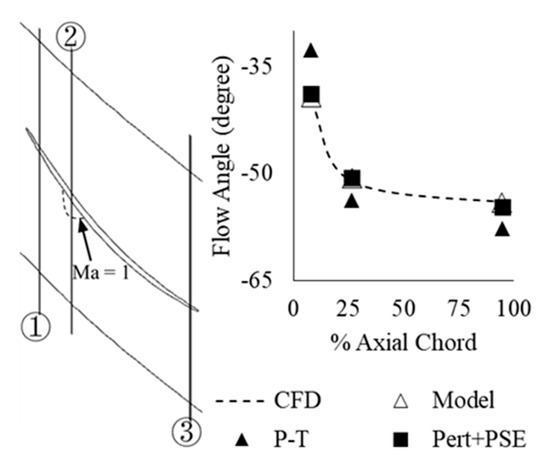
Figure 21.
Model validation results (NASA ADP Fan).
From Figure 21, one can see that even with the transonic flow, Equation (33) still holds. This observation is particularly important as it implies that the effect of shock waves upon the mean flow is via perturbations. Mathematically, this is obvious as the discontinuity induced by the shock wave is that of the first kind, which indicates that the resultant flow-quantity circumferential distributions are integrable.
On the other hand, the component effect of Equation (33) for this cascade shows an entirely different pattern from those of the previous three cascades. In this transonic cascade, the Perturb effect and the PSE effect are predominant throughout the passage as one can see the solid squares almost overlap with the blank triangles, and they both fall right on the curve of CFD results. The balance of these two effects guarantees the flow angle prediction since the P-T effect is minor. This is not the case in the previous three cascades where the P-T effect or the compound of all the three effects together determines the flow angle.
Another finding of the validation in the transonic cascade is that the trailing edge flow field may also be related to the mean flow field directly via total perturbations (Perturb+PSE). Compressors and fans maintained the perturbation dominance near the trailing edge. This again presents large potentials to use wake theory for analysis on discharge flow angles or deviation angles.
4. General Discussion
It is noteworthy that the proposed theory does not explicitly show the effect of viscosity. This poses a potential limitation on its applications at operating conditions such as near stall and may jeopardize the goal of applying the proposed theory to loading–loss modeling. Therefore, how to address viscosity and boundary layer are to be discussed in this section.
4.1. Leading Edge Separations
Note that all the previous analyses are carried out for RANS simulations. That is, all the terms in Equation (30) or Equation (33) are calculated with boundary layer included as parts of the velocity and pressure distributions. The results demonstrated imply that the proposed model can quantify the flow turning without referring to the viscous loss due to the boundary layer. Such a counterintuitive statement stems from the assumption that the viscous dissipation is completely drained by the surface heat transfer [24]. Denton has proved its validity at operating conditions where the Prandtl number is close to unity. When the boundary layer is separated, this assumption is compromised, and hence, Equation (30) or Equation (33) loses its validity thereby. This is confirmed by examining these two equations at off-design conditions. Here, the NASA LPT cascade is taken as an example. Table 6 demonstrates the tested conditions.
Table 6.
Off-design validations conditions on NASA LPT cascade.
Here, only the two axial locations are presented: Locations 1 and 2 in Figure 11. Location 1 resides outside the separation bubble on the suction surface at the design condition (AoA = 2.4o) and inside the bubble at the other two off-design conditions. Location 2, on the other hand, always resides outside the separation bubble regardless of the AoA. The validation results are shown in Figure 22.
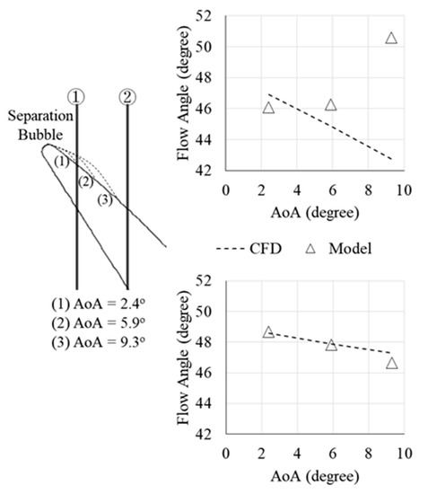
Figure 22.
Validations at off-design conditions: (upper) Location 1; (lower) Locations 2.
Figure 22 shows that, at Location 1, the error of the theory increases as the AoA increases while the error at Location 2 remains marginal. This is exactly as expected since the separations compromised the key assumption for this theory. Specifically, the more separated is the flow, the larger the error is introduced to the theory. To correct this, one needs to rewrite Equation (28) as
The last term in Equation (35) is essentially the term that accounts for the viscous loss. If one enforces the conservations of stagnations enthalpy, the resultant relation will be similar to Equation (30) with an extra term for loss.
From the perspective of modeling, an alternative way to correct this is to regard the separation region, or more precisely the reverse-flow region, as an effective blockage. That is, the boundary curve consisting of zero-axial-velocity points in the bubble is taken as a virtual blade surface, with which all the terms in Equations (30)–(33) are evaluated. Results for such a correction are shown in Figure 23. The agreement is greatly improved compared to the results without the correction. It indicates that Equations (30)–(33) can be coupled with models on separation reattachment to analyze leading-edge flow characteristics, which is of great importance in turbomachinery analysis [36].

Figure 23.
Correction for separation with effective blockage at Location 1.
4.2. Potential Applications
As was observed in the analyses on the NASA E3 cascade and the NASA ADP Fan, the perturbations (Perturb + PSE) may be dominant over the flow angle near the TE. Therefore, it is tempting to use the proposed method and the wake theory to estimate discharge flow angle.
The authors have established a model for predictions of off-design discharge flow angles [37] based on the proposed theory and the wake theory. The model is to relate the perturbations (Perturb + PSE) in the wake region to the inflow conditions. Then off-design flow angles can be evaluated by a scaling relation derived from Equation (33). The model has been validated on both two-dimensional cascade and transonic compressor blade rows. Results showed that the model is of poor accuracy without addressing the viscosity properly and of high accuracy otherwise. Hence, it is essential the in-passage loss can be modeled adequately. Provided that the separation can be modeled as an effective blockage, as presented in the last subsection, the leading-edge stagnation, the blade-surface boundary layers, and the wake downstream can be related to blade loading via Equations (30)–(33) along with corrections on the blockage. The authors are currently working on relating the effective blockage to loss (entropy generation) using the boundary layer theory [38], and it will be the next phase of the research.
5. Concluding Remarks
This paper presents a novel theory that analyzes the flow turning from the perspective of energy balance. The resultant relation(s) shows that three sources contribute to the flow deviation from the mean camber, namely, the pressure-thickness coupling, the perturbation or the covariance of the axial and lateral velocities, and the perturbed stagnation enthalpy. The theory is validated on cascades and blade rows of various types, and the agreement is very good between the theory and the CFD simulation. The contribution of each source is also evaluated. For light-load cascades, the P-T effect is predominant; for subsonic high-load cascades, only the compound of the three effects can determine the correct flow deviation; for transonic cascades, the perturbation and PSE effects together are dominant over the flow. This provides a scope for estimating the in-passage flow for different types of cascades and rows.
The theory addresses the viscosity by balancing it with the blading heat conduction. This measure is effective for operating conditions where the blade-surface boundary layer is stable. When separations or large-scale mixing occurs, the viscous loss must be accounted for proper accuracy. For leading-edge separations, the paper discovered that the reverse-flow region can be regarded as an effective blockage that replaces the blockage factor in Equations (30)–(33). Such a correction yields very accurate predictions on local flow angles based on the proposed theory.
The proposed theory provides a simple tool to quantify in-passage flow characteristics, but it is not a practical tool for predictions or modeling. Along with the precedent work of the authors, however, it is tempting and promising to establish a loss-loading relation that is generally applicable for turbomachineries of various types. The next phase of the research will therefore be to establish the loading–loss relation using the proposed theory and the boundary layer theory.
Author Contributions
Conceptualization, Y.M.; methodology, Y.M.; software, Y.M. and H.L.; validation, Y.M., Z.C. and H.L.; formal analysis, Y.M.; investigation, Y.M.; resources, X.Y.; data curation, Z.C.; writing—original draft preparation, Y.M.; writing—review and editing, Z.C.; visualization, Y.M.; supervision, X.S.; project administration, Y.M. and X.S.; funding acquisition, X.Y. All authors have read and agreed to the published version of the manuscript.
Funding
This work is funded through National Science and Technology Major Project (2017-III-0009-0035) and National Natural Science Foundation of China (Project 51876098 and Project 51911540475).
Institutional Review Board Statement
Not applicable.
Informed Consent Statement
Not applicable.
Data Availability Statement
Data is contained within the article.
Conflicts of Interest
The authors declare no conflict of interest.
Appendix A
For an arbitrary flow quantity , applying moving-average operator (Equation (6)) onto its derivatives, one can have
with Equation (A1), one can derive Equations (9)–(13) from Equations (1)–(5) using simple algebra. The resultant body forces and perturbations are
Nomenclature
| B | blockage factor |
| relative flow angle | |
| c | blade pitch |
| F | body forces |
| γ | angle of attack |
| h | enthalpy |
| I | rothalpy |
| l | chord |
| m | meridional coordinates |
| P | perturbation |
| p | pressure |
| ρ | density |
| θ | circumferential coordinates |
| r | radial coordinate |
| s | entropy |
| T | temperature |
| viscous tensor | |
| u | axial velocity |
| v | lateral velocity |
| x | axial coordinate |
| y | lateral coordinate |
| C | absolute velocity |
| q | heat flux |
| W | relative velocity |
| reference starting point of moving average (linear length) | |
| Superscripts | |
| - | moving averaged quantities |
| ‘ | fluctuation term of the moving-average decomposition |
| ~ | ρ-weighted moving averaged quantities |
| ‘‘ | fluctuation term of the ρ-weighted moving-average decomposition |
| quantities defined over averaged flow field (Equation (29)) | |
| Subscripts | |
| b | blade body force |
| m | meridional streamwise direction |
| p | pressure surface |
| θ | in circumferential direction |
| s | suction surface |
| viscous (loss) force | |
| t | total quantities |
| x | in axial direction |
| Abbreviations | |
| AoA | angle of attack |
| BEP | best efficiency point |
| MFR | mass flow rate |
| NASA | National Aeronautics and Space Administration |
| Re | Reynolds Number |
References
- Wu, C.H. A General Theory of Three-Dimensional Flow in Subsonic and Supersonic Turbomachines of Axial, Radial and Mixed-Flow Types; NACA TN-2604; National Aeronautics and Space Administration: Washington, DC, USA, 1952.
- Lieblein, S. Incidence and Deviation-Angle Correlations for Compressor Cascades. J. Basic Eng. 1960, 82, 575–584. [Google Scholar] [CrossRef]
- Roudebush, W.; Lieblein, S. Viscous Flow in 2D Cascades; NASA SP-36; NASA: Washington, DC, USA, 1965; pp. 151–181.
- Cetin, M.; Uecer, A.S.; Hirsch, C.H.A.R.L.E.S.; Serovy, G.K. Application of Modified Loss and Deviation Correlations to Transonic Axial Compressors; Advisory Group for Aerospace Research and Development (AGARD): Neuilly-Sur-Seine, France, 1987. [Google Scholar]
- König, W.M.; Hennecke, D.K.; Fottner, L. Improved Blade Profile Loss and Deviation Angle Models for Advanced Transonic Compressor Bladings: Part I—A Model for Subsonic Flow. J. Turbomach. 1996, 118, 73–80. [Google Scholar] [CrossRef]
- König, W.M. Improved Blade Profile Loss and Deviation Angle Models for Advanced Transonic Compressor Bladings: Part II—A Model for Supersonic Flow. J. Turbomach. 1996, 118, 81–87. [Google Scholar] [CrossRef]
- Qiu, X.; Japikse, D.; Zhao, J.; Anderson, M.R. Analysis and Validation of a Unified Slip Factor Model for Impellers at Design and Off-Design Conditions. J. Turbomach. 2011, 133, 041018. [Google Scholar] [CrossRef]
- Léonard, O.; Adam, O. A Quasi-One-Dimensional CFD Model for Multistage Turbomachines. J. Thermal Sci. 2008, 17, 7–20. [Google Scholar] [CrossRef]
- Veres, J. Axial and Centrifugal Compressor Mean Line Flow Analysis Method. In Proceedings of the 47th AIAA Aerospace Sciences Meeting including The New Horizons Forum and Aerospace Exposition, Orlando, FL, USA, 5–8 January 2009. [Google Scholar] [CrossRef]
- Boyer, K.M.; O’Brien, W.F. An Improved Streamline Curvature Approach for Off-Design Analysis of Transonic Axial Compression Systems. J. Turbomach. 2003, 125, 475–481. [Google Scholar] [CrossRef]
- Simon, J.F.; Olivier, L. Modeling of 3-D Losses and Deviations in a Throughflow Analysis Tool. J. Thermal Sci. 2007, 16, 208–214. [Google Scholar] [CrossRef]
- Gu, F.; Anderson, M.R. CFD-Based Throughflow Solver in a Turbomachinery Design System. In Proceedings of the ASME Turbo Expo 2007: Power for Land, Sea, and Air, Montreal, QC, Canada, 14–17 May 2007; Volume 6, pp. 1259–1267. [Google Scholar] [CrossRef]
- Pasquale, D.; Persico, G.; Rebay, S. Optimization of Turbomachinery Flow Surfaces Applying a CFD-Based Throughflow Method. J. Turbomach. 2013, 136, 031013. [Google Scholar] [CrossRef]
- Dixon, S.L.; Hall, C.A. Fluid Mechanics and Thermodynamics of Turbomachiner, 7th ed.; Butter-Worth-Heinemann: Oxford, UK, 2014. [Google Scholar]
- Wennestrom, A.J. Design of Highly Loaded Axial-Flow Fans and Compressors; Concepts ETI: White River Junction, VT, USA, 2000. [Google Scholar]
- Dunham, J.; Came, P.M. Improvements to the Ainley-Mathieson Method of Turbine Performance Prediction. J. Eng. Gas Turbine Power 1970, 92, 252–256. [Google Scholar] [CrossRef]
- Kacker, S.C.; Okapuu, U. A Mean Line Prediction Method for Axial Flow Turbine Efficiency. J. Eng. Gas Turbine Power 1982, 104, 111–119. [Google Scholar] [CrossRef]
- Denton, J.D.; Xu, L. The Effects of Lean and Sweep on Transonic Fan Performance. In Proceedings of the ASME Turbo Expo 2002: Power for Land, Sea, and Air, Amsterdam, The Netherlands, 3–6 June 2002; Volume 5, pp. 23–32. [Google Scholar] [CrossRef]
- Lyman, F.A. On the Conservation of Rothalpy in Turbomachines. J. Turbomach. 1993, 115, 520–525. [Google Scholar] [CrossRef]
- Adamczyk, J.J. Model Equation for Simulating Flows in Multistage Turbomachinery; NASA TM-86869; NASA: Washington, DC, USA, November 1985. Available online: https://ntrs.nasa.gov/citations/19850003728 (accessed on 29 August 2021).
- Jennions, I.K.; Stow, P. A Quasi-3D Turbomachinery Blade Design System: Part I: Throughflow Analysis. J. Eng. Gas Turbine Power 1985, 107, 301–307. [Google Scholar] [CrossRef]
- Mao, Y.; Dang, T.Q. A Three-Dimensional Body-Force Model for Nacelle-Fan Systems under Inlet Distortions. Aerosp. Sci. Technol. 2020, 106, 106085. [Google Scholar] [CrossRef]
- Hirsch, C.; Warzee, G. An Integrated Quasi-3D Finite Element Calculation Program for Turbomachinery Flows. J. Eng. Power 1979, 101, 141–148. [Google Scholar] [CrossRef]
- Denton, J.D. The Use of a Distributed Body Force to Simulate Viscous Effects in 3D Flow Calculations. In Proceedings of the ASME 1986 International Gas Turbine Conference and Exhibit, Dusseldorf, Germany, 8–12 June 1986; American Society of Mechanical Engineers: New York, NY, USA, 1986; p. V001T01A058. [Google Scholar] [CrossRef]
- Mao, Y. Body Force Modeling for Engine Inlet Fan System. Ph.D. Thesis, Department of Mechanical and Aerospace Engineering, Syracuse University, Syracuse, NY, USA, 2018. [Google Scholar]
- ANSYS Fluent Theory Guide; ANSYS Inc.: Canonsburg, PA, USA, 2017; Volume 18.1.
- Emery, J.C.; Herrig, L.J.; Erwin, J.R.; Felix, A.R. Systematic Two-Dimensional Cascade Tests of NACA 65-Series Compressor Blades at Low Speed; NACA Report No. 1368; 1958. Available online: https://ntrs.nasa.gov/citations/19930092353 (accessed on 29 August 2021).
- Sharma, O.P.; Kopper, F.C.; Knudsen, L.K.; Yustinich, J.B. Energy Efficient Engine: Low-Pressure Turbine Subsonic Cascade Component Development and Integration Program; NASA CR-165592; NASA: Washington, DC, USA, 1982. Available online: https://ntrs.nasa.gov/citations/19840019670 (accessed on 29 August 2021).
- Marsh, H.; Horlock, J.H. Wall Boundary Layers in Turbomachines. J. Mech. Eng. Sci. 1972, 14, 411–423. [Google Scholar] [CrossRef]
- Kopper, F.C.; Milano, R.; Davis, R.L.; Dring, R.P.; Stoeffler, R.C. High Pressure Turbine Supersonic Cascade Technology Report. NASA CR-165567; 1981. Available online: https://ntrs.nasa.gov/citations/19840019671 (accessed on 29 August 2021).
- Raj, R.; Lakshminarayana, B. Characteristics of the Wake behind a Cascade of Airfoils. J. Fluid Mech. 1973, 61, 707–730. [Google Scholar] [CrossRef]
- Sturrnayr, A.; Hirsch, C. Shock Representation by Euler Throughflow Models and Comparison with Pitch-Averaged Navier-Stokes Solutions. In ISABE Paper 99-7281; Depterment of Fluid Mechanics, Vrije University: Brussels, Belgium, 1999. [Google Scholar]
- Jeracki, R.J. Comprehensive Report of Fan Performance from Duct Rake Instrumentation on 1.294 Pressure Ratio, 806 ft/s Tip Speed Turbofan Simulator Models; NASA TM-2006-213863; NASA: Washington, DC, USA, 2006. Available online: https://ntrs.nasa.gov/citations/20060007570 (accessed on 29 August 2021).
- Tweedt, D.L. Computational Aerodynamic Simulations of an 840 ft/s Tip Speed Advanced Ducted Propulsor Fan System Model for Acoustic Methods Assessment and Development; NASA CR-2014-218129; NASA: Washington, DC, USA, 2014. Available online: https://ntrs.nasa.gov/citations/20140016376 (accessed on 29 August 2021).
- Denton, J.D. The Calculation of Three-Dimensional Viscous Flow through Multistage Turbomachines. J. Turbomach. 1992, 114, 18–26. [Google Scholar] [CrossRef]
- Rosa Taddei, S.; Larocca, F. An Actuator Disk Model of Incidence and Deviation for RANS-Based Throughflow Analysis. J. Turbomach. 2014, 136, 021001. [Google Scholar] [CrossRef]
- Mao, Y.; Su, X.; Yuan, X. An Off-Design Flow Angle Model Based on Average-Flow Theory and Wake Analysis. J. Thermal Sci. 2021. Accepted. [Google Scholar]
- Schlichting, H. Boundary Layer Theory; Springer: Berlin/Heidelberg, Germany, 2017. [Google Scholar]


Publisher’s Note: MDPI stays neutral with regard to jurisdictional claims in published maps and institutional affiliations. |
© 2021 by the authors. Licensee MDPI, Basel, Switzerland. This article is an open access article distributed under the terms and conditions of the Creative Commons Attribution (CC BY) license (https://creativecommons.org/licenses/by/4.0/).