Monte Carlo Based Isogeometric Stochastic Finite Element Method for Uncertainty Quantization in Vibration Analysis of Piezoelectric Materials

Abstract

In this study, a Monte Carlo simulation (MCs)-based isogeometric stochastic Finite Element Method (FEM) is proposed for uncertainty quantification in the vibration analysis of piezoelectric materials. In this method, deterministic solutions (natural frequencies) of the coupled eigenvalue problem are obtained via isogeometric analysis (IGA). Moreover, MCs is employed to solve various uncertainty parameters, including separate elastic and piezoelectric constants and their combined cases.

1. Introduction

Piezoelectric materials are the most widely used smart materials in engineering structures. Their application has reached a mature level, and they have been extensively used in sensors/transducers [1,2,3,4,5,6], energy harvesters [7,8,9] and resonators [10,11,12]. The application of piezoelectric materials is often related to their vibration analysis. Therefore, it is crucial to investigate the effects of electroelastic coupling on the vibration modes of piezoelectric structures. The coupling effect influences the lattice structure of the piezoelectric material and enhances the structure stiffness by a so-called “piezoelectric stiffening” effect [13]. This results in an increase in the natural frequencies of the vibration modes. Piezoelectric ceramics are among primary piezoelectric materials owing to their low price and good coupling. The green body of piezoelectric ceramics is prepared by compression; therefore, the distribution of grain size, density, and local composition is inhomogeneous, resulting in the fluctuation of material parameters [14]. Although some efforts have been made to improve piezoelectric properties [15], the effects of heterogeneity cannot be completely eliminated. Owing to these uncertain factors, the uncertainty quantification of the vibration analysis of piezoelectric materials is extremely important.

Owing to the inability of deterministic analysis to describe random fields, stochastic analysis techniques have been extensively researched to enhance the credibility of computational predictions for uncertainty problems [16]. There are three main approaches to stochastic analysis: perturbation-based techniques [17], stochastic spectral approaches [18,19], and Monte Carlo simulations [20,21,22,23]. Among them, sample-based Monte Carlo simulation (MCs) is considered the most versatile and simple approach. MCs is used to calculate responses from random sampling data to obtain statistical characteristics (expected value, variance, etc.).

Isogeometric analysis (IGA) is an important advancement in computational mechanics and an extension of the Finite Element Method (FEM) [24]. Using the basic features of computer-aided design (CAD), such as Non-Uniform Rational B-splines (NURBS), to discretize the partial differential equations [25,26,27,28,29,30,31,32,33,34,35,36,37,38,39,40,41], one can perform numerical analysis directly from the CAD models, which reduces the preprocessing time for MCs to construct geometric models [23] while maintaining geometric accuracy.

This paper lays out a procedure for solving the uncertainty problems of vibration analysis of piezoelectric materials. This approach consists of two novel points:

• IGA-FEM is employed for the coupled eigenvalue problems of piezoelectric materials.
• We investigate the influence of different factors on coupled eigenvalue problems.

The remainder of the paper is organized as follows. Section 2 gives the fundamentals of MCs in uncertainty quantification. Section 3 presents the isogeometric finite element theory of the vibration analysis of piezoelectric materials. Several numerical examples are provided in Section 4 to obtain the statistical characteristics of the natural frequencies in the vibration analysis of piezoelectric materials, followed by conclusions in Section 5.

2. Uncertainty Quantification Based on Monte Carlo Simulation

Monte Carlo simulation (MCs) is used to directly characterize uncertainty by calculating the expectation and variance of many samples. In general uncertainty quantification, considering a given random field $r\left(X\right)$, the probability density function is $\tilde{\mathcal{P}}\left(r\right)$, and the first two probabilistic moments (expected value and covariance) are defined as follows:

$$\begin{array}{c}\hfill \begin{array}{cc}\hfill & \mathcal{E}\left(r\left(X\right)\right)={\int }_{-\infty }^{+\infty }r\tilde{\mathcal{P}}\left(r\right)\mathrm{d}r,\hfill \\ \hfill & Cov(X,Y)=\mathcal{E}(X-\mathcal{E}(X\left)\right)\mathcal{E}(Y-\mathcal{E}(Y\left)\right).\hfill \end{array}\end{array}$$

(1)

According to the law of large numbers, when more sampling points are selected, the average of the results obtained from multiple sampling points should converge to the desired value, which is the theoretical basis for MCs. Assuming $\tilde{\mathcal{H}}\left(r\right)$ to be an arbitrary function of random variable r. The expected value and variance of $\tilde{\mathcal{H}}\left(r\right)$ can be approximated as:

$$\begin{array}{c}\hfill \begin{array}{cc}\hfill & \mathcal{E}\left[\tilde{\mathcal{H}}\left(r\right)\right]\approx \frac{1}{n_a}\sum _{i=1}^{n_a}{\tilde{\mathcal{H}}}_i\left(r\right),\hfill \\ \hfill & V\left[\tilde{\mathcal{H}}\left(r\right)\right]\approx \frac{1}{n_a-1}\sum _{i=1}^{n_a}{\left[{\tilde{\mathcal{H}}}_i\left(r\right)-\mathcal{E}(\tilde{\mathcal{H}}\left(r\right)\right]}^2.\hfill \end{array}\end{array}$$

(2)

where $n_a$ is the sample size, and the order of convergence rate is $O\left({n_a}^{-1/2}\right)$.

3. Linear Piezoelectricity Vibration Analysis Theory with IGA-FEM

3.1. Linear Piezoelectricity Formulation

For linear piezoelectricity, the electric enthalpy density, $h(S_{ij},E_i)$, is a function of the strain tensor $\mathbf{S}$ and the electric field $\mathbf{E}$, expressed as follows:

$$\begin{array}{c}\hfill h(S_{ij},E_i)=\frac{1}{2}{C}_{ijkl}{S}_{ij}{S}_{kl}-e_{kij}{E}_k{S}_{ij}-\frac{1}{2}{\kappa }_{ij}{E}_i{E}_j,\end{array}$$

(3)

in which $C_{ijkl}$ are the components of the fourth-order elastic tensor $\mathbf{C}$; $e_{kij}$ denote the components of the third-order piezoelectric tensor $\mathbf{e}$; $i,j,k$ and l vary from 1 to 3. The ${\kappa }_{ij}$ are the components of the second-order dielectric tensor $\mathbf{\kappa }$. $E_i$ represent components of electric field $\mathbf{E}$, and $S_{ij}$ are components of strain tensor $\mathbf{S}$. The Stresses/electric displacements $T_{ij}/D_i$ is then defined through the following relations [42]

$$\begin{array}{c}\hfill \begin{array}{cc}\hfill & T_{ij}=\frac{\partial h}{\partial S_{ij}},\hfill \\ \hfill & D_i=-\frac{\partial h}{\partial E_i}.\hfill \end{array}\end{array}$$

(4)

Consider integration over the domain $\mathsf{\Omega }$, the total electrical enthalpy is

$$\begin{array}{c}\hfill H={\int }_{\mathsf{\Omega }}h(S_{ij},E_i)\mathrm{d}\mathsf{\Omega }={\int }_{\mathsf{\Omega }}[\frac{1}{2}{C}_{ijkl}{S}_{ij}{S}_{kl}-e_{kij}{E}_k{S}_{ij}-\frac{1}{2}{\kappa }_{ij}{E}_i{E}_j]\mathrm{d}\mathsf{\Omega }.\end{array}$$

(5)

The generalized geometric equations are given as

$$\begin{array}{cc}\hfill & S_{ij}=\frac{1}{2}[u_{i,j}+u_{j,i}],\hfill \end{array}$$

(6a)

$$\begin{array}{cc}\hfill & E_i=-{\phi }_{,i},\hfill \end{array}$$

(6b)

where $u_i$ are components of displacement $\mathbf{u}$. The ${(·)}_{,i}$ denotes the partial derivative with respect to the coordinate $x_i$. The kinetic energy is defined by

$$\begin{array}{c}\hfill \mathcal{K}\left(\mathbf{u}\right)=\frac{\rho }{2}{\int }_{\mathsf{\Omega }}\frac{\partial u_i}{\partial t}\frac{\partial u_i}{\partial t}\mathrm{d}\mathsf{\Omega },\end{array}$$

(7)

where $\rho$ denotes the mass density per unit volume. The external work is defined by

$$\begin{array}{c}\hfill W_{ext}(\mathbf{u},\phi )={\int }_{{\mathsf{\Gamma }}_t}{u}_i{\overline{f}}_i\mathrm{d}{\mathsf{\Gamma }}_t+{\int }_{{\mathsf{\Gamma }}_d}\omega \phi \mathrm{d}{\mathsf{\Gamma }}_d,\end{array}$$

(8)

where ${\overline{f}}_i$ is the components of mechanical tractions. The value $\omega$ is the surface charge density. ${\mathsf{\Gamma }}_t$ and ${\mathsf{\Gamma }}_d$ are boundaries of $\mathsf{\Omega }$ corresponding to mechanical tractions and electric displacements, respectively.

3.2. IGA-FEM Theory for Linear Piezoelectricity Vibration Analysis

3.2.1. Variational Setting

From Hamilton’s principle, the variation of linear piezoelectricity is expressed as

$$\begin{array}{c}\hfill \delta \left({\int }_{t_0}^{t_1}\mathcal{L}(\mathbf{u},\phi )\mathrm{dt}\right)=0,\end{array}$$

(9)

where $\delta (·)$ represents the variational operator and the Lagrangian is defined as

$$\begin{array}{c}\hfill \mathcal{L}(\mathbf{u},\phi )=\mathcal{K}\left(\mathbf{u}\right)-H(\mathbf{u},\phi )+W_{ext}(\mathbf{u},\phi ).\end{array}$$

(10)

Thus, Equation (9) expands as

$$\begin{array}{c}\hfill \delta {\int }_{t_0}^{t_1}\mathcal{K}\left(\mathbf{u}\right)\mathrm{d}t-\delta {\int }_{t_0}^{t_1}H(\mathbf{u},\phi )\mathrm{d}t+\delta {\int }_{t_0}^{t_1}{W}_{ext}(\mathbf{u},\phi )\mathrm{d}t=0,\end{array}$$

(11)

where the variation of kinetic energy and external work are expressed as

$$\begin{array}{c}\hfill \delta {\int }_{t_0}^{t_1}K\left(\mathbf{u}\right)\mathrm{d}t=-{\int }_{t_0}^{t_1}\rho \left[{\int }_{\mathsf{\Omega }}\delta u_i\frac{{\partial }^2{u}_i}{\partial t^2}\mathrm{d}\mathsf{\Omega }\right]\mathrm{d}t,\end{array}$$

(12)

and

$$\begin{array}{c}\hfill \delta {\int }_{t_0}^{t_1}{W}_{ext}(\mathbf{u},\phi )\mathrm{d}t={\int }_{t_0}^{t_1}\left[{\int }_{{\mathsf{\Gamma }}_t}{\overline{f}}_i\delta u_i\mathrm{d}{\mathsf{\Gamma }}_t+{\int }_{{\mathsf{\Gamma }}_d}\omega \delta \phi \mathrm{d}{\mathsf{\Gamma }}_d\right]\mathrm{d}t.\end{array}$$

(13)

From Equations (5) and (6b), the variation of the total enthalpy is as following

$$\begin{array}{c}\hfill \begin{array}{cc}\hfill \delta {\int }_{t_0}^{t_1}H(\mathbf{u},\phi )\mathrm{d}t=& {\int }_{t_0}^{t_1}\left[{\int }_{\mathsf{\Omega }}{\widehat{C}}_{abcd}\delta S_{ab}{S}_{cd}\mathrm{d}\mathsf{\Omega }\right]\mathrm{d}t+\delta {\int }_{t_0}^{t_1}\left[{\int }_{\mathsf{\Omega }}{\widehat{e}}_{abc}\delta {\phi }_{,a}{S}_{bc}\mathrm{d}\mathsf{\Omega }\right]\mathrm{d}t\hfill \\ \hfill & +\delta {\int }_{t_0}^{t_1}\left[{\int }_{\mathsf{\Omega }}{\widehat{e}}_{abc}{\phi }_{,a}\delta S_{bc}\mathrm{d}\mathsf{\Omega }\right]\mathrm{d}t-\delta {\int }_{t_0}^{t_1}\left[{\int }_{\mathsf{\Omega }}{\widehat{\kappa }}_{ab}\delta {\phi }_{,a}{\phi }_{,b}\mathrm{d}\mathsf{\Omega }\right]\mathrm{d}t.\hfill \end{array}\end{array}$$

(14)

The modified elastic, piezoelectric and dielectric tensors are shown in the Appendix A where $a,b,c$ and d denote the surface variable components. The values for these indicators are 1 and 3. To satisfy Equation (11) for all possible $\delta \mathbf{u}$ and $\delta \phi$, the weak form of the linear piezoelectric vibration analysis controlling equation follows as

$$\begin{array}{c}\hfill \begin{array}{cc}\hfill & {\int }_{\mathsf{\Omega }}\delta u_i\frac{{\partial }^2{u}_i}{\partial t^2}\mathrm{d}\mathsf{\Omega }+{\int }_{\mathsf{\Omega }}{\widehat{C}}_{abcd}\delta S_{ab}{S}_{cd}\mathrm{d}\mathsf{\Omega }+{\int }_{\mathsf{\Omega }}{\widehat{e}}_{abc}\delta {\phi }_{,a}{S}_{bc}\mathrm{d}\mathsf{\Omega }+{\int }_{\mathsf{\Omega }}{\widehat{e}}_{abc}{\phi }_{,a}\delta S_{bc}\mathrm{d}\mathsf{\Omega }\hfill \\ \hfill & -{\int }_{\mathsf{\Omega }}{\widehat{\kappa }}_{ab}\delta {\phi }_{,a}{\phi }_{,b}\mathrm{d}\mathsf{\Omega }-{\int }_{{\mathsf{\Gamma }}_t}\overline{f_i}\delta u_i\mathrm{d}{\mathsf{\Gamma }}_t-{\int }_{{\mathsf{\Gamma }}_d}\omega \delta \phi \mathrm{d}{\mathsf{\Gamma }}_d=0.\hfill \end{array}\end{array}$$

(15)

3.2.2. IGA-FEM Discretization

Given a set of non-decreasing coordinates $\mathsf{\Xi }=[{\xi }_0,{\xi }_1,\dots ,{\xi }_{n+p+1}]$ in the parameter space, and is called the knot vector. The B-spline basis functions are defined as

$$\begin{array}{c}\hfill N_{i,0}\left(\xi \right)=\left\{\begin{array}{cc}1\hfill & \mathrm{if}{\xi }_i\le \xi <{\xi }_{i+1}\\ 0\hfill & \mathrm{otherwise}\end{array}\right.,\end{array}$$

(16)

and

$$N_{i,p}\left(\xi \right)=\frac{\xi -{\xi }_i}{{\xi }_{i+p}-{\xi }_i}{N}_{i,p-1}\left(\xi \right)+\frac{{\xi }_{i+p+1}-\xi }{{\xi }_{i+p+1}-{\xi }_{i+1}}{N}_{i+1,p-1}\left(\xi \right),$$

(17)

where $\xi$ denotes the parametric coordinate, n is the number of basis functions, and p is the polynomial order. Figure 1 gives an example of a k-refinement of a B-spline, in which different color lines represent different basis functions. From this example, we can intuitively feel the richness of B-spline functions in IGA. Considering the control points ${\mathbf{P}}_{i,j}\in \mathbb{R}{}^d$, all parametric spaces can be reduced to a unit interval (d = 1), square (d = 2) or cube (d = 3) [43]. In this paper, d is set to be 2. Considering two knot vectors ${\mathsf{\Xi }}^1=[{\xi }_0,{\xi }_1,\dots ,{\xi }_{n+p+1}]$ and ${\mathsf{\Xi }}^2=[{\eta }_0,{\eta }_1,\dots ,{\eta }_{m+q+1}]$ and control points ${\mathbf{P}}_{i,j}\in \mathbb{R}{}^d$, a B-spline surface is defined as

$$\overline{\mathbf{S}}(\xi ,\eta )=\sum _{i=1}^n\sum _{j=1}^m{N}_{i,p}\left(\xi \right)M_{j,q}\left(\eta \right){\mathbf{P}}_{i,j},$$

(18)

where $N_{i,p}$ and $M_{j,q}$ are univariate B-spline basis functions with polynomial order p and q, respectively. The NURBS surface is defined with the following:

$$\tilde{\mathbf{S}}(\xi ,\eta )=\sum _{i=1}^n\sum _{j=1}^m{R}_{i,j}^{p,q}(\xi ,\eta ){\mathbf{P}}_{i,j},$$

(19)

and

$$R_{i,j}^{p,q}(\xi ,\eta )=\frac{N_{i,p}\left(\xi \right)M_{j,q}\left(\eta \right){\mathcal{W}}_{i,j}}{{\displaystyle \sum _{i^{\prime }=1}^n}{\displaystyle \sum _{j^{\prime }=1}^m}{N}_{i^{\prime },p}\left(\xi \right)M_{i^{\prime },q}\left(\eta \right){\mathcal{W}}_{i^{\prime },j^{\prime }}},$$

(20)

where $R_{i,j}^{p,q}(\xi ,\eta )$ are the bivariate NURBS basis functions, ${\mathcal{W}}_i$ is referred to as the ith weight. The displacement and electric potential $\phi$ are discretized using the NURBS basis functions as

$$\begin{array}{c}\hfill \mathbf{u}=\sum _{B=0}^{n_b-1}{N}_B{\mathbf{U}}_B,\phi =\sum _{B=0}^{n_b-1}{N}_B{\mathsf{\Phi }}_B,\end{array}$$

(21)

where $n_b$ is the number of basis functions. ${\mathbf{U}}_B$ is the Bth nodal coefficients of displacement, and the ${\mathsf{\Phi }}_B$ represents the nodal coefficients of the electric potential.

From Equation (6a), the strain components are computed as

$$S_{ab}=\sum _B^{n_b-1}\frac{1}{2}[N_{B,b}+N_{B,a}]·{\mathbf{U}}_B.$$

(22)

Following a Bubnov-Galerkin method, the NURBS basis functions are also used for the $\delta \mathbf{u}$ and $\delta \phi$, and Equation (15) can be written as [44]

$$\begin{array}{c}\hfill \left[\begin{array}{cc}\mathrm{M}& 0\\ 0& 0\end{array}\right]\left\{\begin{array}{c}\ddot{\mathrm{u}}\hfill \\ 0\hfill \end{array}\right\}+\left[\begin{array}{cc}\mathrm{K}& {\mathrm{C}}_{u\phi }\\ {\mathrm{C}}_{\phi u}& {\mathrm{D}}_{\phi \phi }\end{array}\right]\left\{\begin{array}{c}\mathrm{u}\hfill \\ \psi \hfill \end{array}\right\}=\left\{\begin{array}{c}{\mathrm{f}}_u\hfill \\ {\mathrm{f}}_{\phi }\hfill \end{array}\right\},\end{array}$$

(23)

where $\mathrm{M}$ is the global mass matrix. The value $\ddot{\mathrm{u}}$ represents global acceleration vector. $\mathrm{K}$ is the global stiffness matrix, ${\mathrm{D}}_{\phi \phi }$ represents the global dielectric system matrix, ${\mathrm{C}}_{u\phi }$ and ${\mathrm{C}}_{\phi u}$ denote the direct and converse piezoelectric coupling matrices, respectively. Values $\mathrm{u}$ and $\psi$ are the global vectors of displacement, and electric potential coefficients, respectively. Values ${\mathrm{f}}_u$ and ${\mathrm{f}}_{\phi }$ are the global structural and electrical load vectors. To improve the computational efficiency, the Schur complement ${\mathrm{C}}_{u\phi }{\mathrm{D}}_{\phi \phi }^{-1}{\mathrm{C}}_{\phi u}$ is used to modify the system of equations. Thus, the problem for $\mathrm{u}$ can be written as

$$\begin{array}{c}\hfill \begin{array}{c}\hfill \mathrm{M}\ddot{\mathrm{u}}+[\mathrm{K}-{\mathrm{C}}_{u\phi }{\mathrm{D}}_{\phi \phi }^{-1}{\mathrm{C}}_{\phi u}]\mathrm{u}={\mathrm{f}}_u-{\mathrm{C}}_{u\phi }{\mathrm{D}}_{\phi \phi }^{-1}{\mathrm{f}}_{\phi }.\end{array}\end{array}$$

(24)

Then, the new global system matrices are defined as

$$\begin{array}{c}\hfill \begin{array}{c}\hfill \mathrm{A}=\mathrm{K}-{\mathrm{C}}_{u\phi }{\mathrm{D}}_{\phi \phi }^{-1}{\mathrm{C}}_{\phi u}.\end{array}\end{array}$$

(25)

The system of equations is thus defined as

$$\begin{array}{c}\hfill \begin{array}{c}\hfill \mathrm{M}\ddot{\mathrm{u}}+\mathrm{A}\mathrm{u}={\mathrm{f}}_u-{\mathrm{C}}_{u\phi }{\mathrm{D}}_{\phi \phi }^{-1}{\mathrm{f}}_{\phi }.\end{array}\end{array}$$

(26)

The free vibration problem of linear piezoelectricity can be obtained by assuming harmonic motions, and the expression is

$$\begin{array}{c}\hfill \begin{array}{c}\hfill [-{\overline{\omega }}^2\mathrm{M}+\mathrm{A}]\mathrm{u}={\mathrm{f}}_u-{\mathrm{C}}_{u\phi }{\mathrm{D}}_{\phi \phi }^{-1}{\mathrm{f}}_{\phi },\end{array}\end{array}$$

(27)

where $\overline{\omega }$ is the angular frequency. For the free vibration analysis problem, by setting the external mechanical and electrical loads to zero, the above equation can be reduced as

$$\begin{array}{c}\hfill \begin{array}{c}\hfill [-{\overline{\omega }}^2\mathrm{M}+\mathrm{A}]=0.\end{array}\end{array}$$

(28)

4. Numerical Examples

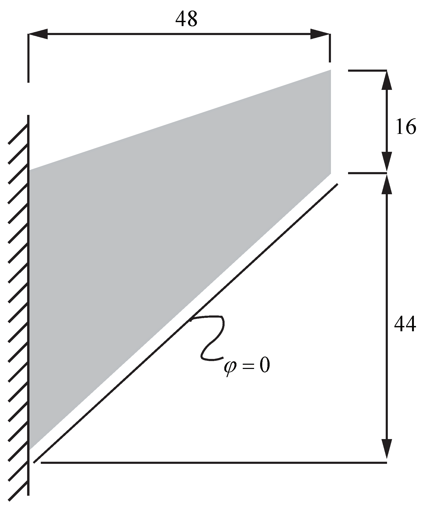
4.1. Piezoelectric Tapered Panel

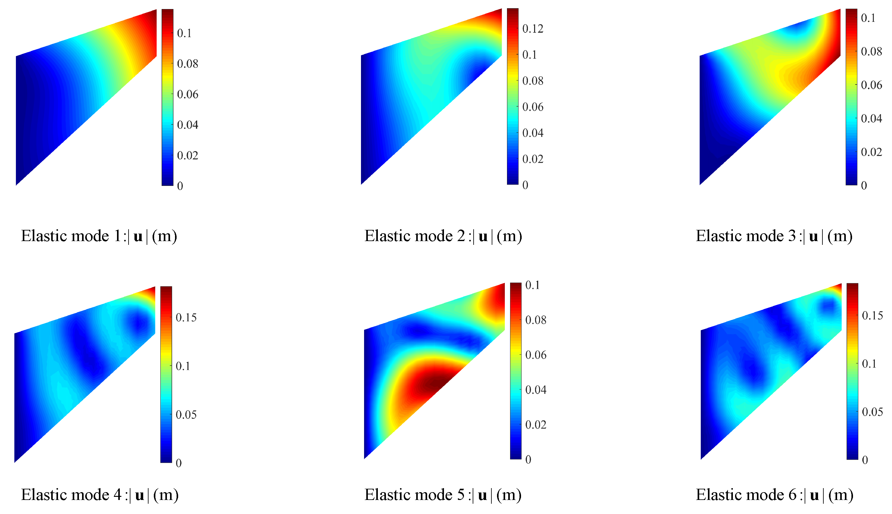
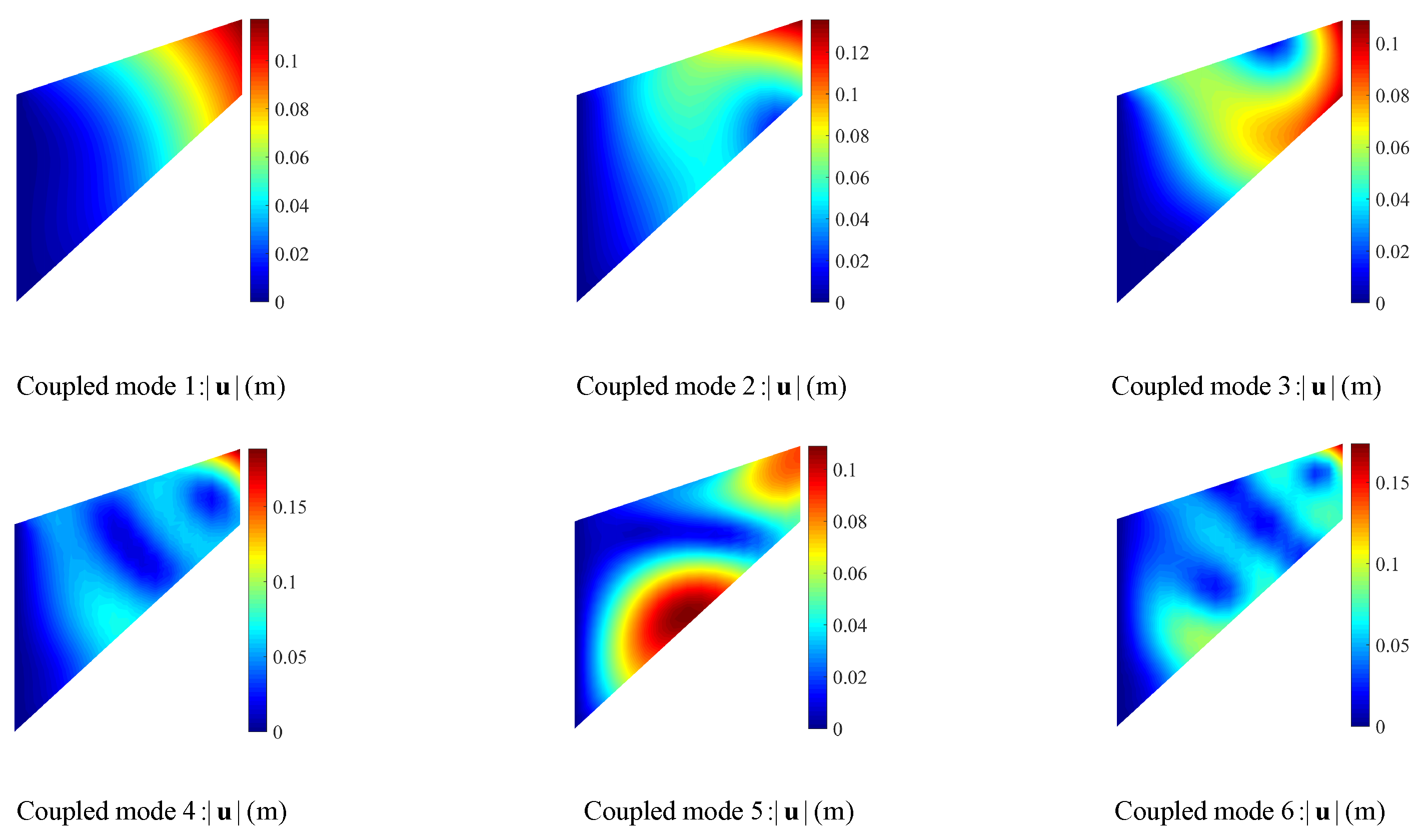
4.1.1. Piezoelectric Tapered Panel Free Vibration Analysis

In this section, the free-vibration analysis of a clamped tapered panel model is discussed, as shown in Figure 2. The boundary conditions are similar to those of cantilever structures. The PZT-4 piezoelectric material is used to create this model, and the material parameters are listed in

Table 1. Material parameters for tapered panel.

Name	PZT-4
Mass density $\rho$	7500 kg/m${}^3$
Elastic constants
$C_{1111}$	139 GPa
$C_{1122}$	77.8 GPa
$C_{1133}$	74 GPa
$C_{3333}$	115 GPa
$C_{1313}$	25.6 GPa
Piezoelectric constants
$e_{113}$	12.7 C/m${}^2$
$e_{311}$	−5.2 C/m${}^2$
$e_{333}$	15.7 C/m${}^2$
Permittivity
${\kappa }_{11}$	6.46 × 10${}^{-9}$ C/(Vm)
${\kappa }_{33}$	5.62 × 10${}^{-9}$ C/(Vm)

. Nine initial control points are considered, and the coordinates and weights for these control points are listed in

Table 2. Control point coordinates and weights for the tapered panel.

i	${\mathit{P}}_{\mathit{i},1}$ (mm, mm)	${\mathit{P}}_{\mathit{i},2}$ (mm, mm)	${\mathit{P}}_{\mathit{i},3}$ (mm, mm)	${\mathcal{W}}_{\mathit{i},1}$	${\mathcal{W}}_{\mathit{i},2}$	${\mathcal{W}}_{\mathit{i},3}$
1	(0, 0)	(24, 22)	(48, 44)	1	1	1
2	(0, 22)	(24, 37)	(48, 52)	1	1	1
3	(0, 44)	(24, 52)	(48, 60)	1	1	1

. The lower surface electric potential is specified as 0V. FEM employs the traditional Lagrangian basis functions, which generally require many mesh divisions to obtain high accuracy, but the computational efficiency is low. However, IGA-FEM uses the NURBS basis functions to ease the preprocessing time by increasing the order, thus improving the computational efficiency. This is the fundamental reason for choosing IGA-FEM in this paper.

Figure 3 shows the first six displacement eigenmodes of a purely elastic problem for the tapered structure. Figure 4 and Figure 5 show the first six eigenmodes of the piezoelectric tapered structure. The magnitude of the displacement and electric potential function $\phi$ distribution on the tapered panel are plotted. Compared to the purely elastic tapered panel, the modal displacement did not exhibit a notable change.

Table 3. Comparison of natural frequency IGA results for elastic and electroelastic coupling of tapered panel.

Eigenvalue Number	Elastic (Hz)	Piezoelectric Coupled (Hz)
1	3.90 × 10${}^4$	4.23 × 10${}^4$
2	1.00 × 10${}^5$	1.19 × 10${}^5$
3	1.21 × 10${}^5$	1.28 × 10${}^5$
4	2.00 × 10${}^5$	2.29 × 10${}^5$
5	2.55 × 10${}^5$	2.73 × 10${}^5$
6	2.83 × 10${}^5$	3.09 × 10${}^5$

lists the natural frequencies of the elastic and electroelastic coupling problems. As can be seen from Table 3, the coupling effect causes an increase in the eigenmode frequency, known as “piezoelectric stiffening”.

4.1.2. Uncertainty Quantification for Piezoelectric Tapered Panel Model with MCs

In this section, the tapered panel model presented in Section 4.1.1, is selected for uncertainty quantization models. We consider the elastic constant $C_{111}$ and piezoelectric constant $e_{333}$ as random input variables. These random variables satisfy the expected values $\mu$ = 1.39 × 10${}^{11}$ and $\mu =15.1$ Gaussian distribution and the standard deviation $\sigma =\mu \times \gamma$, where $\gamma$ represents the coefficient of variation. The natural frequency has a large influence on the stability of the structure. Therefore, in this paper, we investigate the factors influencing the natural frequency of piezoelectric materials.

Table 4. Definitions and the statistical properties of the random input variables ($\gamma =0.02$ and 0.06).

Random Input Variables	$\mathit{\mu }$	The Limits of Input Variables: [Lower, Upper]
		$\mathit{\gamma }$ = 0.02	$\mathit{\gamma }$ = 0.06
$C_{1111}$	1.39 × 10 ${}^{11}$	[1.31 × 10${}^{11}$, 1.46 × 10${}^{11}$]	[1.14 × 10${}^{11}$, 1.66 × 10${}^{11}$]
$e_{333}$	15.1	[14.3, 16.2]	[12.2, 17.7]

and

Table 5. Definitions and the statistical properties of the random input variables ($\gamma =0.1$, 0.14, and 0.18).

Random Input Variables	$\mathit{\mu }$	The Limits of Input Variables: [Lower, Upper]
		$\mathit{\gamma }$ = 0.1	$\mathit{\gamma }$ = 0.14	$\mathit{\gamma }$ = 0.18
$C_{1111}$	1.39 × 10${}^{11}$	[8.96 × 10${}^{10}$, 1.85 × 10${}^{11}$]	[8.59 × 10${}^{10}$, 2.08 × 10${}^{11}$]	[7.81 × 10${}^{10}$, 2.17 × 10${}^{11}$]
$e_{333}$	15.1	[10.5, 19.5]	[9.1, 20.8]	[7.5, 22.0]

list all the input parameters with their range, where the scale of the datasets is determined according to the $3\sigma$ principle.

Table 6. Size of the samples.

Dimension of Input	Variable	Samples
Variables		(${\mathit{n}}_{\mathit{a}}$,${\mathit{n}}_{\mathit{a}}$)
1-D	$C_{1111}$	(500, 500)
	$e_{333}$	(500, 500)
2-D	$C_{1111}$+$e_{333}$	(${25}^2$, 625)

gives the size of samples for single random input variable denoted by “1-D” and multidimensional input variables “2-D”, respectively. The number of sampling points denoted by $n_a$ is chosen as 500 for “1-D” analysis, but ${25}^2$ for “2-D” analysis. The computational efficiency of Monte Carlo simulation depends on the size of the sample points, too few sample points cannot guarantee the computational accuracy while too many sample points reduce the computational efficiency. We found through experimental comparison that 500 sample points can guarantee the computational accuracy while ensuring the computational efficiency. In the multidimensional input variables analysis, we increased the number of sample points to verify the effect of sample point fluctuations. When the number of samples increases, the calculation accuracy can be improved, but the calculation efficiency becomes worse.

Figure 6 and Figure 7 show the expected values and standard deviations of the second and fourth nonzero eigenvalues (natural frequency) under different coefficients of variation. This includes a single random variable, $C_{1111}$ or $e_{333}$ and the two combined case. It can be observed from these figures that the variation in the piezoelectric constants had little effect on the expected values and standard deviations of the responses. Notably, the standard deviation was the largest when considering the uncertainty of the single random variable $C_{1111}$ and increased rapidly with an increase in the coefficient of variation. Therefore, fluctuations in elastic constants significantly affect the dynamic characteristics of piezoelectric structures.

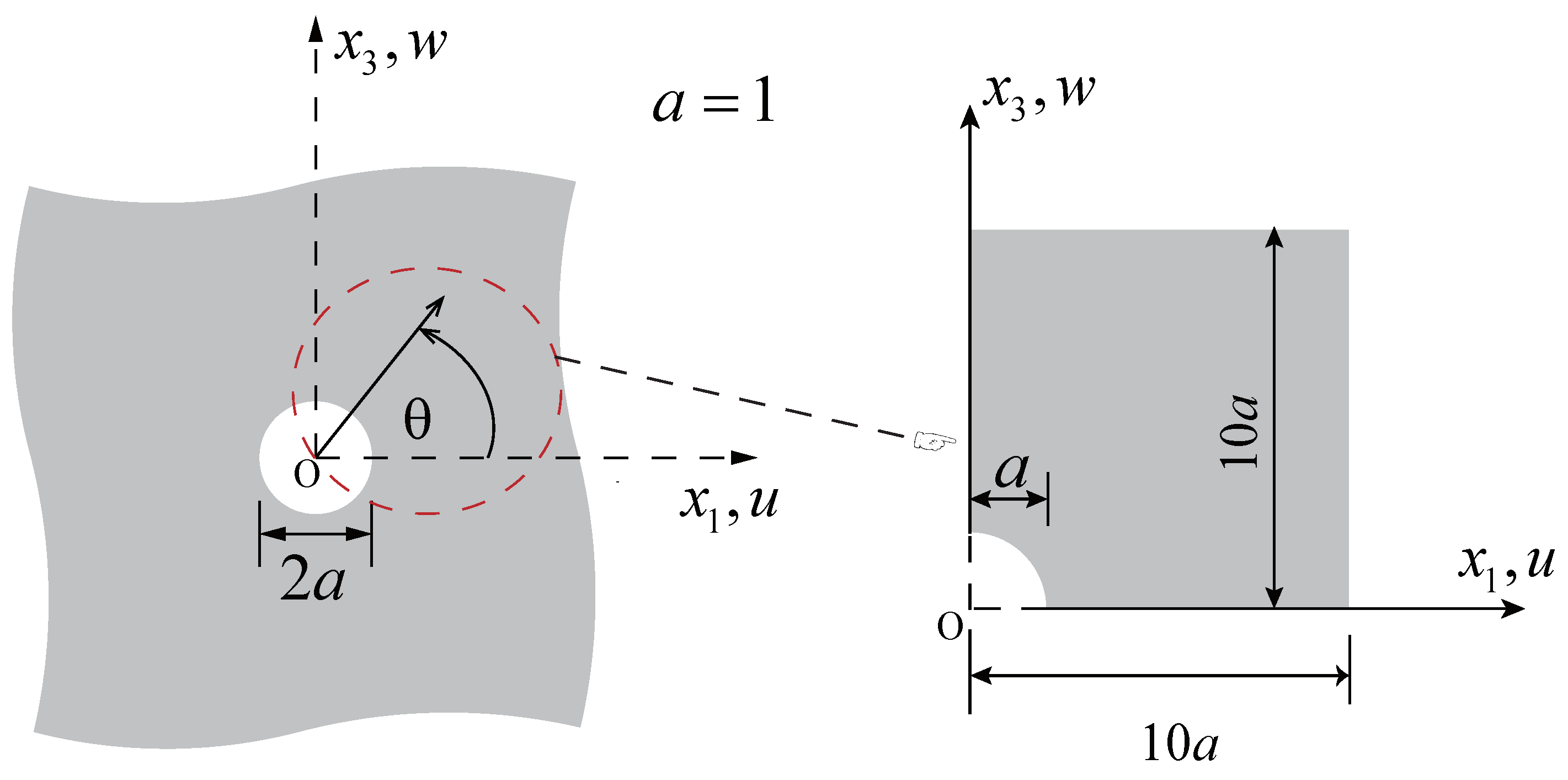
4.2. Infinite Plate with Circular Hole

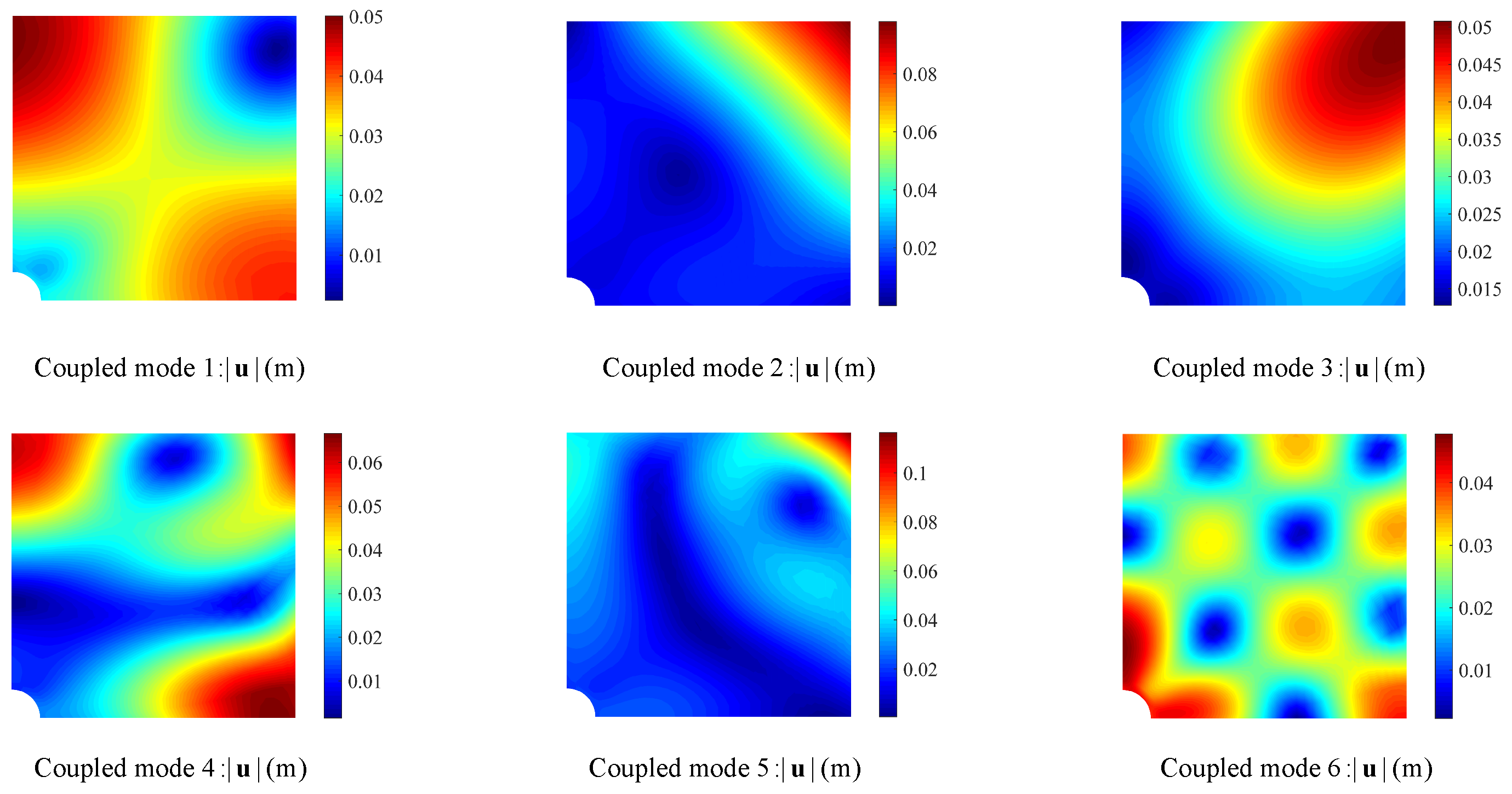
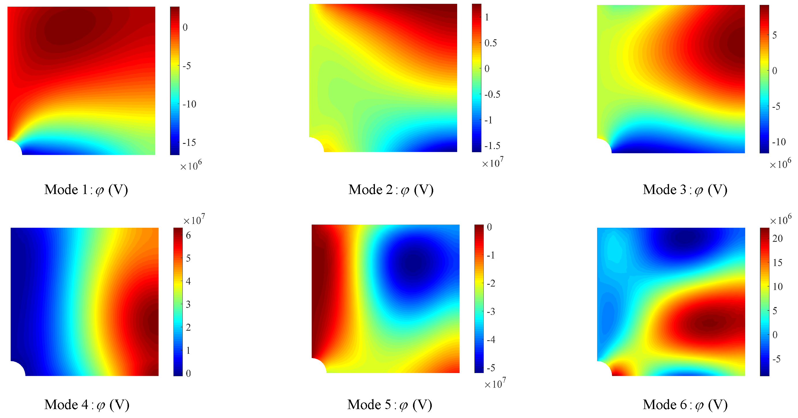
4.2.1. Infinite Plate with Circular Hole Free Vibration Analysis

In this section, we examine the influence of the coupling effects on the natural frequencies and eigenmodes using an infinite plate with a circular hole. The detailed material parameters are listed in

Table 7. Material parameters for infinite plate with circular hole.

Name	PZT-5H
Mass density $\rho$	7500 kg/m${}^3$
Elastic constants
$C_{1111}$	126 GPa
$C_{1122}$	79.1 GPa
$C_{1133}$	83.9 GPa
$C_{3333}$	117 GPa
$C_{1313}$	23 GPa
Piezoelectric constants
$e_{113}$	17.0 C/m${}^2$
$e_{311}$	−6.5 C/m${}^2$
$e_{333}$	23.3 C/m${}^2$
Permittivity
${\kappa }_{11}$	1.505 × 10${}^{-8}$ C/(Vm)
${\kappa }_{33}$	1.302 × 10${}^{-8}$ C/(Vm)

. Owing to the symmetry of the infinite plate, a quarter-plate model with a quarter-hole is employed, as shown in Figure 8. The size of the quarter-plate is much larger than that of the hole. The control points on the left edge have only one translational DoF of the $x_3$-direction and the control points on the bottom edge have only one translational DoF of the $x_1$-direction, i.e., sliding supports are applied on the symmetrical edges of the quarter-plate model. The electric potential on the left surface of the quarter-plate is prescribed as 0 V. The coarsest mesh, ${\mathsf{\Xi }}^1\times {\mathsf{\Xi }}^2$, is defined by the knot vector ${\mathsf{\Xi }}^1={\mathsf{\Xi }}^2=[0,0,0,0.5,1,1,1]$. The control point relationships are listed in

Table 8. Control point coordinates and weights for the plate with a circular hole.

i	${\mathit{P}}_{\mathit{i},1}$ (mm, mm)	${\mathit{P}}_{\mathit{i},2}$ (mm, mm)	${\mathit{P}}_{\mathit{i},3}$ (mm, mm)	${\mathit{P}}_{\mathit{i},4}$ (mm, mm)	${\mathcal{W}}_{\mathit{i},1}$	${\mathcal{W}}_{\mathit{i},2}$	${\mathcal{W}}_{\mathit{i},3}$	${\mathcal{W}}_{\mathit{i},4}$
1	(0, 1)	(0, 3.4278)	(0, 7.75)	(0, 10)	1	1	1	1
2	(0.4142, 1)	(0.5954, 3.4278)	(5.375, 7.75)	(10, 10)	0.8536	1	1	1
3	(1, 0.4142)	(3.4278, 0.5954)	(7.75, 5.375)	(10, 10)	0.8536	1	1	1
4	(1, 0)	(3.4278, 0)	(7.75, 0)	(10, 0)	1	1	1	1

. We selected this sample size in Section 4.1.2.

The distributions for the first six eigenmodes of the purely elastic and coupled problems are shown in Figure 9 and Figure 10. The distribution of eigenmodes of the electric potential is shown in Figure 11. It can be seen from these figures that distribution of displacement eigenmodes were approximately the same for the purely elastic problem and the coupled problem. The first six eigenvalues (natural frequencies) of the purely elastic and coupled problems are listed in

Table 9. Comparison of natural frequency IGA results for elastic and electroelastic coupling of infinite plate with circular hole.

Eigenvalue Number	Elastic (Hz)	Piezoelectric Coupled (Hz)
1	3.33 × 10${}^5$	3.46 × 10${}^5$
2	4.13 × 10${}^5$	4.28 × 10${}^5$
3	5.23 × 10${}^5$	5.34 × 10${}^5$
4	7.26 × 10${}^5$	8.10 × 10${}^5$
5	8.49 × 10${}^5$	9.26 × 10${}^5$
6	1.01 × 10${}^5$	1.05 × 10${}^5$

. From the results, we can still observe the piezoelectric “stiffening effect”.

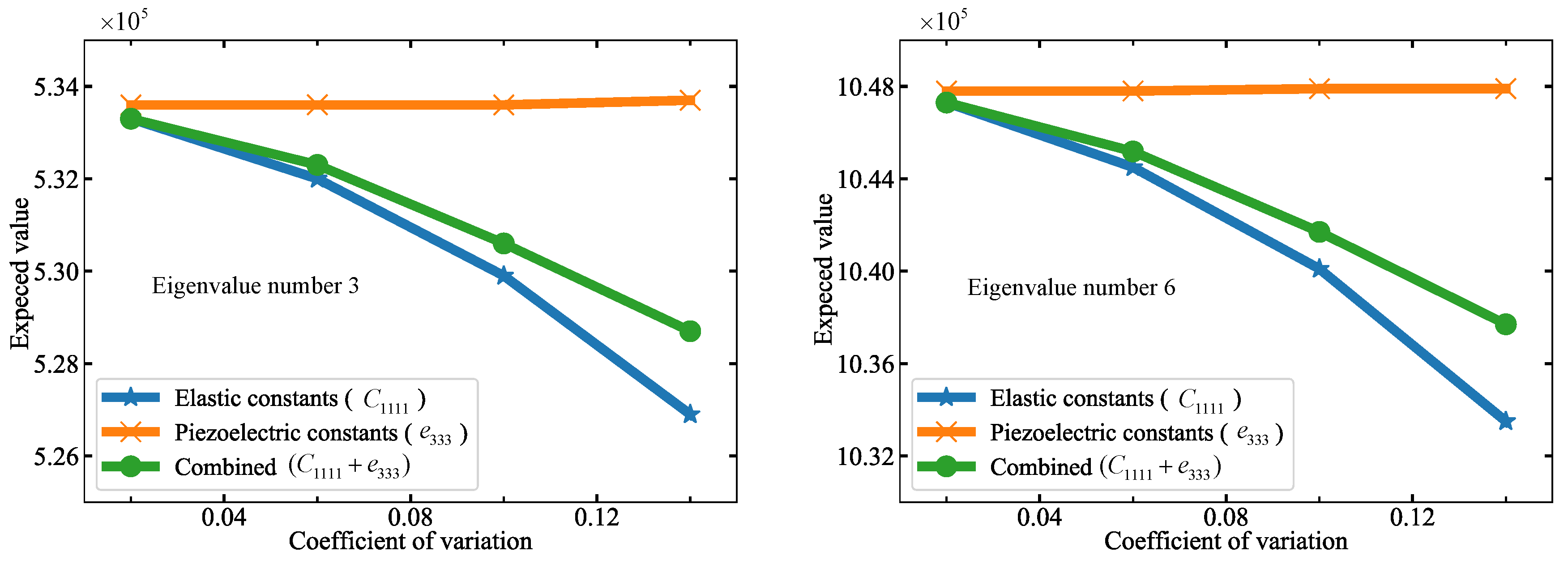
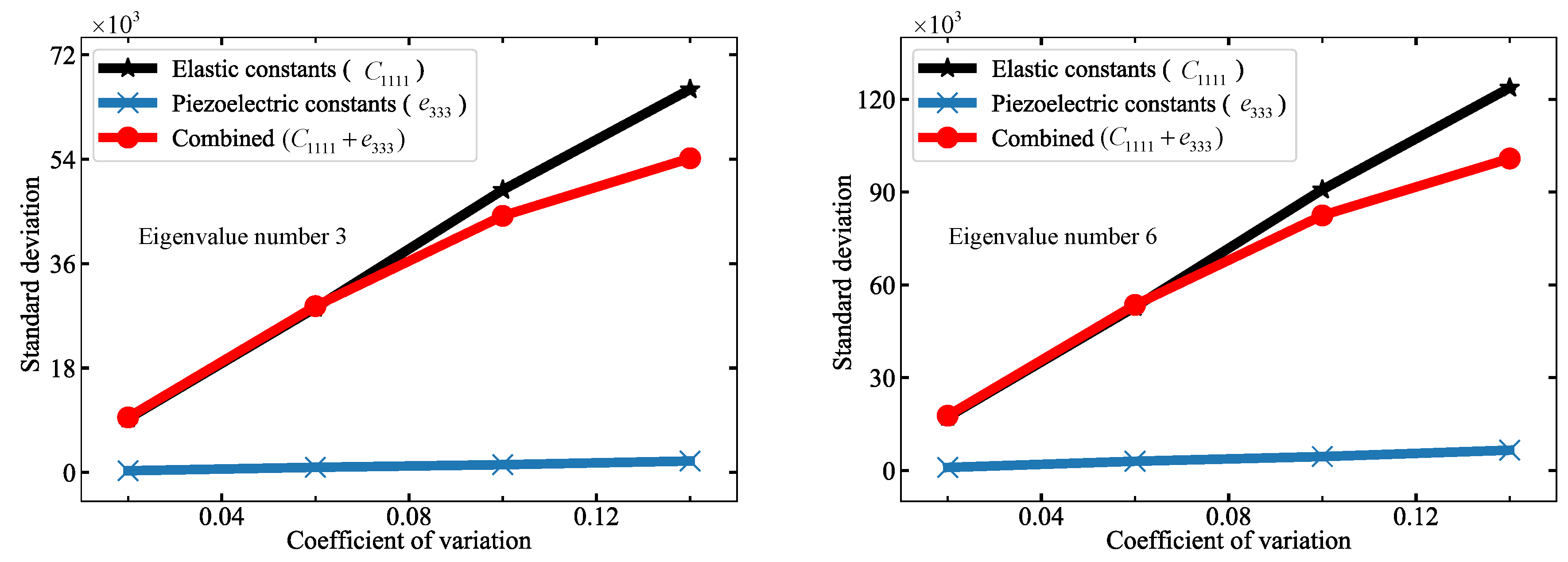
4.2.2. Uncertainty Quantification for Infinite Plate with Circular Hole Model with MCs

In this section, we further investigate the effect of the coefficient of variation on the eigenvalues (natural frequencies) of the coupled problem using an infinite plate with a hole model. We selected $C_{1111}$ and $e_{333}$ as random variables. The expected values of these random variables were $\mu$ = 1.26 × 10${}^{11}$ and $\mu$ = 23.3, and they satisfied the Gaussian distribution.

Table 10. Definitions and the statistical properties of the random input variables ($\gamma =0.02$ and 0.06).

Random Input Variables	Symbol	$\mathit{\mu }$	The Limits of Input Variables: [Lower, Upper]
			$\mathit{\gamma }$ = 0.02	$\mathit{\gamma }$ = 0.06
Elastic constants	$C_{1111}$	1.26 × 10${}^{11}$	[1.18 × 10${}^{11}$, 1.33 × 10${}^{11}$]	[1.04 × 10${}^{11}$, 1.53 × 10${}^{11}$]
piezoelectric constants	$e_{333}$	23.3	[22.0, 24.8]	[19.1, 29.0]

and

Table 11. Definitions and the statistical properties of the random input variables ($\gamma =0.1$ and 0.14).

Random Input Variables	Symbol	$\mathit{\mu }$	The Limits of Input Variables: [Lower, Upper]
			$\mathit{\gamma }$ = 0.1	$\mathit{\gamma }$ = 0.14
Elastic constants	$C_{1111}$	1.26 × 10${}^{11}$	[8.86 × 10${}^{10}$, 1.61 × 10${}^{11}$]	[8.06 × 10${}^{10}$, 1.72 × 10${}^{11}$]
piezoelectric constants	$e_{333}$	23.3	[17.3, 31.0]	[12.9, 34.1]

list all the input parameters with their range, where the scale of the datasets is determined according to the 3$\sigma$ principle.

In this problem, we examined the third and sixth non-zero eigenvalues. For the elastic constant $C_{1111}$, piezoelectric constant $e_{333}$, and their combinations, the expected values and standard deviations of the responses in relation to the coefficient of variation are shown in Figure 12 and Figure 13, respectively. It can be observed that the expected values and standard deviations of the responses are similar to the results obtained from the tapered panel model in Section 4.1.2. The statistical characteristics of the natural frequencies in the vibration analysis of piezoelectric materials are better reflected by different examples.

5. Conclusions

In this study, a Monte Carlo simulation-based isogeometric stochastic Finite Element Method was used for uncertainty quantification in the vibration analysis of piezoelectric materials. The smoothness of the IGA basis functions was used to discretize the governing equations of the coupled problem. The IGA-FEM eliminates repetitive meshing procedure in uncertainty quantification and retains geometric accuracy. In general, the natural frequencies of piezoelectric structures are higher than that in the absence of piezoelectric effects. This “piezoelectric stiffening” effect is crucial for certain modes. By comparing the statistical characteristics of the natural frequencies, the fluctuations in the elastic constants have the greatest impact on the results of the statistical characteristics in the three cases. According to the numerical cases, the change in dielectric constants has a negligible effect on the expected values and standard deviations of the natural frequencies. Additionally, the present method will be applied to three-dimensional piezoelectric problems, two-dimensional and three-dimensional flexoelectric problems.

References

1. Redwood, M. Transient performance of a piezoelectric transducer. J. Acoust. Soc. Am. 1961, 33, 527–536. [Google Scholar] [CrossRef]
2. Jaffe, H.; Berlincourt, D. Piezoelectric transducer materials. Proc. IEEE 1965, 53, 1372–1386. [Google Scholar] [CrossRef]
3. Abboud, T.; Nédélec, J.; Zhou, B. Improvement of the integral equation method for high frequency problems. In Proceedings of the Third International Conference on Mathematical Aspects of Wave Propagation Phenomena, SIAM, Mandelieu-La Napoule, France, 24–28 April 1995; pp. 178–187. [Google Scholar]
4. Tzou, H.; Tseng, C. Distributed piezoelectric sensor/actuator design for dynamic measurement/control of distributed parameter systems: A piezoelectric finite element approach. J. Sound Vib. 1990, 138, 17–34. [Google Scholar] [CrossRef]
5. Ng, T.; Liao, W. Sensitivity analysis and energy harvesting for a self-powered piezoelectric sensor. J. Intell. Mater. Syst. Struct. 2005, 16, 785–797. [Google Scholar] [CrossRef]
6. Safari, A.; Akdogan, E.K. Piezoelectric and Acoustic Materials for Transducer Applications; Springer Science & Business Media: New York, NY, USA, 2008. [Google Scholar]
7. Erturk, A.; Inman, D.J. Piezoelectric Energy Harvesting; John Wiley & Sons: Hoboken, NY, USA, 2011. [Google Scholar]
8. Kim, H.S.; Kim, J.H.; Kim, J. A review of piezoelectric energy harvesting based on vibration. Int. J. Precis. Eng. Manuf. 2011, 12, 1129–1141. [Google Scholar] [CrossRef]
9. Hurtado, A.C.; Peralta, P.; Ruiz, R.; Alamdari, M.M.; Atroshchenko, E. Shape optimization of piezoelectric energy harvesters of variable thickness. J. Sound Vib. 2022, 517, 116503. [Google Scholar] [CrossRef]
10. Benes, E.; Hammer, D. Piezoelectric resonator with acoustic reflectors. J. Acoust. Soc. Am. 1980, 67, 750. [Google Scholar] [CrossRef]
11. Nowotny, H.; Benes, E. General one-dimensional treatment of the layered piezoelectric resonator with two electrodes. J. Acoust. Soc. Am. 1987, 82, 513–521. [Google Scholar] [CrossRef]
12. Hollkamp, J.J. Multimodal passive vibration suppression with piezoelectric materials and resonant shunts. J. Intell. Mater. Syst. Struct. 1994, 5, 49–57. [Google Scholar] [CrossRef]
13. Johannsmann, D. Piezoelectric stiffening. In The Quartz Crystal Microbalance in Soft Matter Research; Springer: New York, NY, USA, 2015; pp. 125–142. [Google Scholar]
14. Rahaman, M.N.; De Jonghe, L.C.; Chu, M.Y. Effect of green density on densification and creep during sintering. J. Am. Ceram. Soc. 1991, 74, 514–519. [Google Scholar] [CrossRef]
15. Chen, P.; Yi, K.; Liu, J.; Hou, Y.; Chu, B. Effects of density inhomogeneity in green body on the structure and properties of ferroelectric ceramics. J. Mater. Sci. Mater. Electron. 2021, 32, 16554–16564. [Google Scholar] [CrossRef]
16. Stefanou, G. The stochastic finite element method: Past, present and future. Comput. Methods Appl. Mech. Eng. 2009, 198, 1031–1051. [Google Scholar] [CrossRef] [Green Version]
17. Kamiński, M. Generalized perturbation-based stochastic finite element method in elastostatics. Comput. Struct. 2007, 85, 586–594. [Google Scholar] [CrossRef]
18. Ghanem, R.G.; Spanos, P.D. Stochastic Finite Elements: A Spectral Approach; Courier Corporation: Chelmsford, MA, USA, 2003. [Google Scholar]
19. Chen, N.Z.; Soares, C.G. Spectral stochastic finite element analysis for laminated composite plates. Comput. Methods Appl. Mech. Eng. 2008, 197, 4830–4839. [Google Scholar] [CrossRef]
20. Hurtado, J.; Barbat, A. Monte Carlo techniques in computational stochastic mechanics. Arch. Comput. Methods Eng. 1998, 5, 3–29. [Google Scholar] [CrossRef]
21. Spanos, P.D.; Zeldin, B.A. Monte Carlo Treatment of Random Fields: A Broad Perspective. Appl. Mech. Rev. 1998, 51, 219–237. [Google Scholar] [CrossRef]
22. Feng, Y.; Li, C.; Owen, D. A directed Monte Carlo solution of linear stochastic algebraic system of equations. Finite Elem. Anal. Des. 2010, 46, 462–473. [Google Scholar] [CrossRef]
23. Chen, L.; Cheng, R.; Li, S.; Lian, H.; Zheng, C.; Bordas, S.P. A sample-efficient deep learning method for multivariate uncertainty qualification of acoustic–vibration interaction problems. Comput. Methods Appl. Mech. Eng. 2022, 393, 114784. [Google Scholar] [CrossRef]
24. Hughes, T.; Cottrell, J.; Bazilevs, Y. Isogeometric analysis: CAD, finite elements, NURBS, exact geometry and mesh refinement. Comput. Methods Appl. Mech. Eng. 2005, 194, 4135–4195. [Google Scholar] [CrossRef] [Green Version]
25. Chen, L.; Lian, H.; Liu, Z.; Chen, H.; Atroshchenko, E.; Bordas, S. Structural shape optimization of three dimensional acoustic problems with isogeometric boundary element methods. Comput. Methods Appl. Mech. Eng. 2019, 355, 926–951. [Google Scholar] [CrossRef]
26. Yu, B.; Cao, G.; Meng, Z.; Gong, Y.; Dong, C. Three-dimensional transient heat conduction problems in FGMs via IG-DRBEM. Comput. Methods Appl. Mech. Eng. 2021, 384, 113958. [Google Scholar] [CrossRef]
27. González-Rodelas, P.; Pasadas, M.; Kouibia, A.; Mustafa, B. Numerical Solution of Linear Volterra Integral Equation Systems of Second Kind by Radial Basis Functions. Mathematics 2022, 10, 223. [Google Scholar] [CrossRef]
28. Chen, L.; Marburg, S.; Zhao, W.; Liu, C.; Chen, H. Implementation of Isogeometric Fast Multipole Boundary Element Methods for 2D Half-Space Acoustic Scattering Problems with Absorbing Boundary Condition. J. Theor. Comput. Acoust. 2019, 27, 1850024. [Google Scholar] [CrossRef] [Green Version]
29. Chen, L.; Lu, C.; Zhao, W.; Chen, H.; Zheng, C. Subdivision Surfaces - Boundary Element Accelerated by Fast Multipole for the Structural Acoustic Problem. J. Theor. Comput. Acoust. 2020, 28, 2050011. [Google Scholar] [CrossRef]
30. Chen, L.; Zhang, Y.; Lian, H.; Atroshchenko, E.; Ding, C.; Bordas, S.P. Seamless integration of computer-aided geometric modeling and acoustic simulation: Isogeometric boundary element methods based on Catmull-Clark subdivision surfaces. Adv. Eng. Softw. 2020, 149, 102879. [Google Scholar] [CrossRef]
31. Ibáñez, M.J.; Barrera, D.; Maldonado, D.; Yáñez, R.; Roldán, J.B. Non-Uniform Spline Quasi-Interpolation to Extract the Series Resistance in Resistive Switching Memristors for Compact Modeling Purposes. Mathematics 2021, 9, 2159. [Google Scholar] [CrossRef]
32. Chen, L.; Lian, H.; Natarajan, S.; Zhao, W.; Chen, X.; Bordas, S. Multi-frequency acoustic topology optimization of sound-absorption materials with isogeometric boundary element methods accelerated by frequency-decoupling and model order reduction techniques. Comput. Methods Appl. Mech. Eng. 2022, 395, 114997. [Google Scholar] [CrossRef]
33. Wang, L.; Xiong, C.; Yuan, X.; Wu, H. Discontinuous Galerkin Isogeometric Analysis of Convection Problem on Surface. Mathematics 2021, 9, 497. [Google Scholar] [CrossRef]
34. Chen, L.; Liu, C.; Zhao, W.; Liu, L. An isogeometric approach of two dimensional acoustic design sensitivity analysis and topology optimization analysis for absorbing material distribution. Comput. Methods Appl. Mech. Eng. 2018, 336, 507–532. [Google Scholar] [CrossRef]
35. Yu, B.; Cao, G.; Huo, W.; Zhou, H.; Atroshchenko, E. Isogeometric dual reciprocity boundary element method for solving transient heat conduction problems with heat sources. J. Comput. Appl. Math. 2021, 385, 113197. [Google Scholar] [CrossRef]
36. Peng, X.; Atroshchenko, E.; Kerfriden, P.; Bordas, S.P.A. Linear elastic fracture simulation directly from CAD: 2D NURBS-based implementation and role of tip enrichment. Int. J. Fract. 2017, 204, 55–78. [Google Scholar] [CrossRef]
37. Yu, P.; Bordas, S.P.A.; Kerfriden, P. Adaptive Isogeometric analysis for transient dynamics: Space–time refinement based on hierarchical a-posteriori error estimations. Comput. Methods Appl. Mech. Eng. 2022, 394, 114774. [Google Scholar] [CrossRef]
38. Peng, X.; Atroshchenko, E.; Kerfriden, P.; Bordas, S.P.A. Isogeometric boundary element methods for three dimensional static fracture and fatigue crack growth. Comput. Methods Appl. Mech. Eng. 2017, 316, 151–185. [Google Scholar] [CrossRef] [Green Version]
39. Chen, L.; Li, K.; Peng, X.; Lian, H.; Lin, X.; Fu, Z. Isogeometric Boundary Element Analysis for 2D Transient Heat Conduction Problem with Radial Integration Method. Comput. Model. Eng. Sci. 2021, 126, 125–146. [Google Scholar] [CrossRef]
40. Chen, L.; Wang, Z.; Peng, X.; Yang, J.; Wu, P.; Lian, H. Modeling pressurized fracture propagation with the isogeometric BEM. Geomech. Geophys. Geo-Energy Geo-Resour. 2021, 7, 1–16. [Google Scholar] [CrossRef]
41. Chen, L.; Lian, H.; Liu, Z.; Gong, Y.; Zheng, C.; Bordas, S. Bi-material topology optimization for fully coupled structural-acoustic systems with isogeometric FEM–BEM. Eng. Anal. Bound. Elem. 2022, 135, 182–195. [Google Scholar] [CrossRef]
42. Ghasemi, H.; Park, H.S.; Rabczuk, T. A level-set based IGA formulation for topology optimization of flexoelectric materials. Comput. Methods Appl. Mech. Eng. 2017, 313, 239–258. [Google Scholar] [CrossRef]
43. Nguyen, V.P.; Anitescu, C.; Bordas, S.P.; Rabczuk, T. Isogeometric analysis: An overview and computer implementation aspects. Math. Comput. Simul. 2015, 117, 89–116. [Google Scholar] [CrossRef] [Green Version]
44. Nguyen, V.T.; Kumar, P.; Leong, J.Y.C. Finite Element Modelling and Simulations of Piezoelectric Actuators Responses with Uncertainty Quantification. Computation 2018, 6, 60. [Google Scholar] [CrossRef] [Green Version]
Figure 1. An example of k-refinement of B-spline, in which different color lines represent different basis functions.
Mathematics 10 01840 g001
Figure 2. The free-vibration analysis of a clamped tapered panel model.
Mathematics 10 01840 g002
Figure 3. Eigenmodes distribution of purely elastic displacement of tapered panel structure.
Mathematics 10 01840 g003
Figure 4. Eigenmodes distribution of coupled displacement of tapered panel structure.
Mathematics 10 01840 g004
Figure 5. Eigenmodes distribution of electric potential of the tapered panel structure.
Mathematics 10 01840 g005
Figure 6. Expected values for separate C 1111 , e 333 and the two uncertainties combined case with different coefficient of variation (tapered panel model).
Mathematics 10 01840 g006
Figure 7. Standard variation for separate C 1111 , e 333 and the two uncertainties combined case with different coefficient of variation (tapered panel model).
Mathematics 10 01840 g007
Figure 8. Infinite plate with circular hole model.
Mathematics 10 01840 g008
Figure 9. Eigenmodes distribution of purely elastic displacement of a quarter plate with circular hole.
Mathematics 10 01840 g009
Figure 10. Eigenmodes distribution of coupled displacement of a quarter plate with circular hole.
Mathematics 10 01840 g010
Figure 11. Eigenmodes distribution of electric potential of a quarter plate with circular hole.
Mathematics 10 01840 g011
Figure 12. Expected values for separate C 1111 , e 333 and the two uncertainties combined case with different coefficient of variation (one-fourth of the plate model).
Mathematics 10 01840 g012
Figure 13. Standard variation for separate C 1111 , e 333 and the two uncertainties combined case with different coefficient of variation (one-fourth of the plate model).
Mathematics 10 01840 g013