Graph-Based Integration of Histone Modification Profiles

Abstract

In this work, we introduce a similarity-network-based approach to explore the role of interacting single-cell histone modification signals in haematopoiesis—the process of differentiation of blood cells. Histones are proteins that provide structural support to chromosomes. They are subject to chemical modifications—acetylation or methylation—that affect the degree of accessibility of genes and, in turn, the formation of different phenotypes. The concentration of histone modifications can be modelled as a continuous signal, which can be used to build single-cell profiles. In the present work, the profiles of cell types involved in haematopoiesis are built based on all the major histone modifications (i.e., H3K27ac, H3K27me3, H3K36me3, H3K4me1, H3K4me3, H3K9me3) by counting the number of peaks in the modification signals; then, the profiles are used to compute modification-specific similarity networks among the considered phenotypes. As histone modifications come as interacting signals, we applied a similarity network fusion technique to integrate these networks in a unique graph, with the aim of studying the simultaneous effect of all the modifications for the determination of different phenotypes. The networks permit defining of a graph-cut-based separation score for evaluating the homogeneity of subgroups of cell types corresponding to the myeloid and lymphoid phenotypes in the classical representation of the haematopoietic tree. Resulting scores show that separation into myeloid and lymphoid phenotypes reflects the actual process of haematopoiesis.

1. Introduction

Histones are basic proteins which bind tightly to DNA in the nuclei of eukaryotic cells. According to the ‘beads-on-a-string’ model [1], they combine into octamers to form nucleosomes, the basic units around which DNA wraps to form chromatin. The nucleosomes, in turn, bind together to form a chain structure that constitutes the backbone of the three-dimensional arrangement of chromosomes.

Some residues of histone proteins, namely lysines and arginines, represent possible targets for post-translational modifications, such as methylation and acetylation [2]. Moreover, particular patterns of histone modifications are interpreted as a code specifying for genetic functions [3,4]. Although parts of the working principles of this code are being investigated, most of it still represents a puzzle for biologists, as well as a computational challenge for bioinformaticians. However, the existence of an intrinsic relationship between the three-dimensional structure of chromosomes, gene accessibility and gene expression has been highlighted [5]. Consequently, histone modifications emerge as fundamental epigenetic agents for the development of different cell phenotypes. The advent of the cost-effective ChIP-seq technology [6] that combines chromatin immunoprecipitation and massively parallel sequencing, and the consequent large availability of data, have made it possible to read the traces of all the histone modifications of the genome [7]. Accordingly, several institutions—which came together to form the International Human Epigenome Consortium (IHEC) (https://ihec-epigenomes.org/) [8]—have teamed up to generate huge databases of such epigenetic markers.

In this paper, we show how histone modification traces can be turned into whole-genome profiles. This is achieved by identifying and counting high-resolution peaks (steep local maxima with sizes as small as a hundred bps) in the histone modification signal. The obtained profiles show behaviour that resembles that of gene expression, with only a small fraction of genes exhibiting relevant activity (relatively high peak counts), and the vast majority being silent. Indeed, the existence of a tight relationship between histone modifications and transcription has been deeply investigated, and quantitative models to predict the expression level of genes from histone modification levels have been derived. It is well-known, in fact, that histone modification levels and gene expression are highly correlated, while only a small number of histone modifications are necessary to accurately predict gene expression [5,9,10]. Consequently, it is possible to borrow methods from differential expression analysis to extract knowledge from histone modification profiles (see, for example, [11]). In particular, the proposed model integrates the information contained in all the histone modification signals involved in haematopoiesis (see https://epigenomesportal.ca/ihec/grid.html?build=2020-10&assembly=4&cellTypeCategories=1, accessed on 23 March 2022). This choice is based on the observation that a single modification may not be able to capture the complexity of epigenetics, since a phenotype is the result of the combination of contrasting contributions—promotion or repression—of several modifications [12].

Initially, the information contained in each histone modification is treated separately, constructing a dissimilarity network of cell types; then, all the networks are integrated using a similarity network fusion technique [13,14]. This integration model is suitable for several applications, including that of clustering a population of cell types into homogeneous groups. Nevertheless, if the sought sub-populations are unknown, it could be useful to compare alternative partitions of the population into subgroups rather than performing clustering. Following this idea, we define a score to quantitatively evaluate the plausibility of a graph bipartition into two subgroups of vertices. The combination of the integration model with the evaluation score for graph bipartitions is then tested by considering a hypothesis on the biological process of haematopoiesis, i.e., the process of the formation of all blood cells from a common progenitor. Specifically, we tested the classical hypothesis on the existence of two main subpopulations of cell types in haematopoiesis, namely the lymphoid and myeloid cells [15]. Figure 1 depicts an outline of the proposed methodology.

The paper is organised as follows. In Section 2, the adopted method is described. In Section 3, the experimental analysis and the obtained results are presented. A discussion of the methodology and the results is offered in Section 4. Finally, some conclusions are given in Section 5.

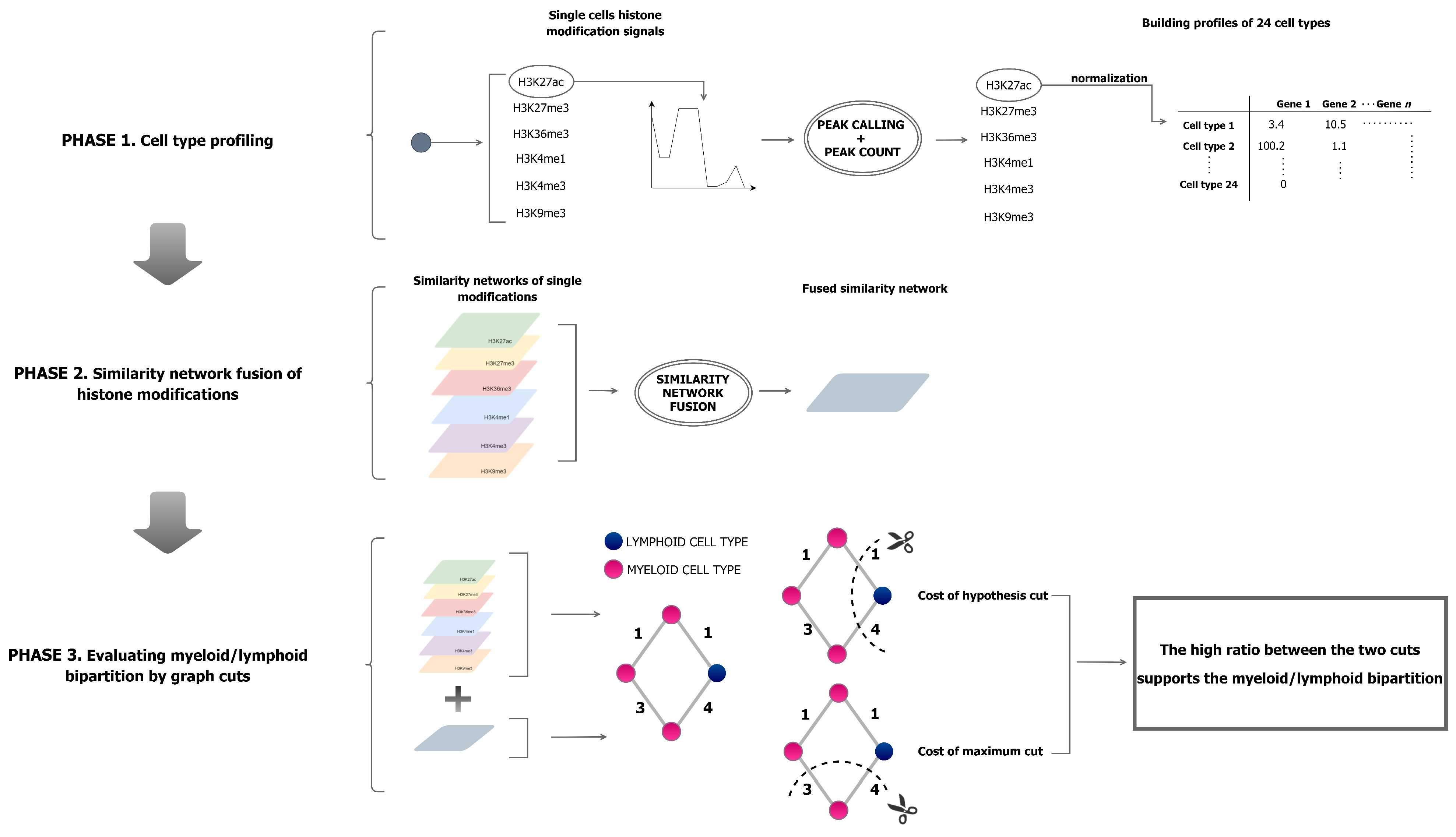
2. Materials and Methods

A histone modification track has the form of a continuous signal. The signal is obtained after a first phase of ChIP-sequencing by associating each nucleotide of the DNA sequence with the number of reads of the modifier covering it [7]. In this section, we first show how to detect and count peaks in these signals in order to build the histone modification profiles of a cell. Moreover, we describe how cell-type profiles from different histone modifications can be organised into a network-based setup and then integrated into a unique, comprehensive graph. Finally, we propose a graph-cut-based hypothesis testing scheme for evaluating graph bipartitions.

2.1. Peak Calling

Let $X=\{x_1,\dots ,x_n\}$ be the histone modification track of a sample cell X, where the value $x_i$ corresponds to the number of supporting reads covering genomic position i. Intuitively, a peak is a contiguous region around a local maximum in track X. More specifically, the peak region consists of two monotone curves leading to a point whose value is the highest within a neighbourhood of points. From this informal definition, two free parameters can be derived to define a peak: (i) its height and (ii) its width. Despite being simple in principle, these two parameters make finding peaks complicated. Indeed, different settings, as well as appropriate algorithms, may be required for specific applications. For instance, setting large surrounding areas is equivalent to seeking large peaks (low-resolution peaks), which are suitable for the identification of genomic sites involved in histone modification. This is the case, for example, of Sole-Search [16], the peak detection algorithm used at IHEC [8]. On the other hand, searching for small peaks (high-resolution peaks) is more appropriate for quantification. Since the first step of this analysis aims at quantifying the number of peaks in a histone modification track, we design an algorithm to identify high resolution peaks (with resolution on the order of a few bps).

Let $X_h=\{{\widehat{x}}_1,\dots ,{\widehat{x}}_{n/h}\}$ be a transformation of profile X at resolution h, where ${\widehat{x}}_i=mean\left([x_{hi},\dots ,x_{(h+1)i-1}]\right)$. Let $R\left(X_h\right)=\{r_1,\dots ,r_m\}$ ($m\le n/h$) be a compact representation of $X_h$, where consecutive pairs ${\widehat{x}}_i$ and ${\widehat{x}}_{i+1}$ are merged if ${\widehat{x}}_i={\widehat{x}}_{i+1}$. An element $r_i$ is eligible as a peak if it satisfies, at least, the conditions $r_i>r_{i-1}$ and $r_i>r_{i+1}$. The representation of a histone modification track $X_h$ with $R\left(X_h\right)$ allows us to consider all the maxima as candidate peaks independent of their width. Thence, in order for a point $r_i$ to be a real peak, two additional features are required. First, the signal increase has to be steep enough. Second, the candidate $r_i$ has to be compared with its background. To this end, as a background we use the interval $I\left(r_i\right)=[\alpha ,\beta ]$, where $\alpha$ and $\beta$ are integer numbers such that $\alpha <i<\beta$ and $r_{\alpha -1}=0$, $r_{\beta +1}=0$, and $r_j\ne 0$$\forall j\in [\alpha <i<\beta ]$, while the peak intensity is computed as the Z-score of $r_i$, where:

$$z\left(r_i\right)=\frac{r_i-\mu \left(I\left(r_i\right)\right)}{\sigma \left(I\left(r_i\right)\right)},$$

(1)

$\mu \left(\right)$ denotes the mean, and $\sigma \left(\right)$ is the standard deviation of the signal distribution over the interval $I\left(\right)$. The Z-score defined in Equation (1) does not depend on the scale of the histone modification signal and has the advantage of being interpretable as a sort of fold change. Consequently, a peak can be defined as a genomic locus where the score $z\left(\right)$ is higher than a user-defined threshold (set to 2 in our experiments).

2.2. Normalisation

After the peak-calling step, we proceed by counting the number of peaks for each gene. Peak counting, as many other quantification tasks from NGS data, is influenced by sequencing depth. Indeed, in order for a peak to be individuated, it has to be endowed with a consistent number of supporting reads. This generally happens easily with strong signals, while it requires high coverage for weaker signals. Counts per million (CPM) and reads per kilobase per million [17] (RPKM) are two widespread normalisation methods used in the field of RNA-seq to mitigate the effect of sequencing productivity. Both methods leverage on the acceptable assumption that the overall amount of signals (in this case, peaks) per sample is roughly constant. The main difference between CPM and RPKM is that the latter is based on the additional assumption that the molar concentration of RNA is constant. Consequently, the number of reads per gene is proportional to gene length. In the context of this work, CPM and RPKM assume slightly different semantics. CPM is based on the hypothesis that a cell phenotype is determined only by the presence of a high concentration of a histone modification signals. It is therefore an absolute measure of concentration of histone modification peaks inside a gene. In contrast, RPKM is a relative measure, as it relies on the idea that the determination of a cell phenotype depends on the distribution of the number of peaks along the gene. Hence, in the latter case, it is assumed that a high concentration of histone modifications is not sufficient in itself to produce a phenotype, but rather must be spread along the gene.

Due to the lack of evidence to support a model based on the absolute concentration of histone modifications or relative concentration, both CPM and RPKM are tested in our experiments.

2.3. Cell-Type Expression Profiles

The IHEC data portal [8] makes a variable number of different samples available for a given cell type. Such redundant information can be exploited to build a unique profile for each phenotype, which, in turn, has the effect of mitigating possible bias due to the intrinsic variability of samples. In this work, this is achieved by taking the average of the per-gene contributions of profiles of the same cell type.

Similarly to gene expression, it is reasonable to assume that most genes do not contribute to a phenotype of interest because they are expressed constantly or not at all. In a framework where the computation of similarity/distance between phenotypes is required, the effect of these genes would be that of pushing the ratio between the two nearest and the two furthest elements towards 1. Consequently, it would be complicated to look for differentiated subgroups of phenotypes. Since we are interested in computing similarities/distances between different cell types, a strategy for filtering out those genes is required. Nevertheless, it is difficult to establish a priori a cutoff threshold to filter out infrequently expressed genes, as genes with similar profiles could be excluded only on the basis of a negligible distance from the threshold. In order to solve this issue, we choose to cluster genes, and to interpret each cluster centroid as representing all the group members. In this way, a whole cluster is either retained or filtered out based on the profile of its centroid. In this work, the clustering of genes is performed using the k-means algorithm, and the centroids are initialised using the Lloyd procedure [18] (the implementation is available via the R [19] function kmeans). The number of clusters k is set to 50 (thanks to a raw grid search based on the elbow method [20]) to ensure high within-cluster homogeneity, which is required for removing or retaining genes with similar profiles. Finally, we set a conservative threshold for filtering out clusters of genes with constant or no expression [21]. More precisely, a cluster is retained only if the maximum value of its centroid is higher than the lowest 10% of the expression interval.

2.4. Profile Integration

Histone modifications exert their effects directly by influencing the overall structure of chromatin, promoting or inhibiting gene accessibility. As a result, a phenotype can be seen as a combination of all the contributions of the single modifications. Based on this observation, we present a strategy that integrates the information of similarities/dissimilarities between profiles of cell types coming from several modifications into a unique similarity/dissimilarity network. In order to perform profile integration, the Similarity Network Fusion (SNF) [14] algorithm (the software can be downloaded in R or MATLAB versions at http://compbio.cs.toronto.edu/SNF/SNF/Software.html, accessed on 23 March 2022) is exploited. The input to SNF consists of a set of similarity networks, one for each histone modification, characterised by the same set of vertices (cell types). Then, by applying a cross-diffusion process (CrDP) [13], SNF outputs a unique weighted similarity graph with the same set of nodes as the original networks. In brief, the algorithm iteratively updates the single similarity networks by promoting (i) strong links, which are not necessarily present in all the networks, and (ii) weak links that are shared by all the networks. Then, at the final iteration step, the contributions of the single networks are averaged to define a unique similarity graph. The resulting network can therefore give information on how multiple variables determine similarities among cell types.

2.5. Hypothesis Testing

The model described in Section 2.4 is applied to graphs where nodes are cell types, and edges are weighted with a similarity value between pairs of cell types. With the aim of studying how to divide the nodes of these graphs into two homogeneous groups, we define a notion of separation by using graph cuts. A sensible bipartition of a similarity network should have low-weighted edges between the two distinct sets and relatively higher-weighted edges within the groups. Thus, the cost of a cut constitutes quantitative information on the level of separation of the graph components. In line with this observation, it is possible to define a score that is proportional to the degree of separation between two groups, a task easier to carry out with dissimilarity graphs. Dissimilarities can be easily computed starting from similarities. For example, a dissimilarity weight can be obtained by first converting similarities into Z-scores and then inverting them with respect to the mean.

Applying a cut to a dissimilarity network is not in itself sufficient to determine the goodness of a network bipartition. In fact, a lower and an upper bound on the cost of a cut induced by a partition must be introduced. In principle, setting the lower and the upper bound as the costs, respectively, of the minimum and the maximum cut might be a reasonable choice. However, the two scores are highly dependent on the weight values and the graph topology. Therefore, they do not represent a good solution when scores obtained for different graphs have to be compared. In order to get rid of these scaling problems, the separation measure can be converted into a scale-free score as follows:

$$S\left(h\right)=\frac{\lambda \left(h\right)-{min}_{c\in C\left(G\right)}\lambda \left(c\right)}{{max}_{c\in C\left(G\right)}\lambda \left(c\right)-{min}_{c\in C\left(G\right)}\lambda \left(c\right)},$$

(2)

where $C\left(G\right)$ denotes the set of all possible graph cuts of graph G, $\lambda \left(\right)$ denotes the cost function of a cut, and h is the cut induced by the bipartition to be evaluated (referred to as the hypothesis cut). The score $S\left(h\right)$ takes on values in the range $[0,1]$ and reaches its maximum when the cost of the hypothesis cut reaches that of the maximum cut on G (the similarities between vertices of the same group are high and those among vertices of different groups are low). Computation of the maximum cut represents a major issue for computing $S\left(h\right)$. Indeed, while exact algorithms for computing the minimum cut exist [22,23], computation of the maximum cut is known to be an $NP$-complete [24] problem. However, heuristic solutions can be adopted to find the solution.

In this work, the maximum cut approach is implemented in the R environment following the Greedy Cut Algorithm proposed in [25]. As for the min-cut, we use the R function min_cut from the igraph package, which is an implementation of the algorithm proposed in [26].

In our experiments, the score is tested on dissimilarity networks of cell types with the aim of studying if two subpopulations appear to have substantially different phenotypes.

3. Results

3.1. Dataset

The experimental analysis is conducted by using whole-genome histone modification profiles from a collection of cell samples involved in haematopoiesis (the complex differentiation process that starts from stem cells and gives origin to all types of blood cells).

The data come from the 2020-10 release by the Blueprint project (https://www.blueprint-epigenome.eu/), and are available at the International Human Epigenome Consortium (IHEC) [8] data portal (https://epigenomesportal.ca/ihec/). The dataset consists of 1254 samples of 35 distinct cell types, each registering six modification marks on histone H3. The marks are identified by the Roadmap Epigenome Mapping Centers (http://www.roadmapepigenomics.org/). More specifically, the histone modifications include mono and tri-methylation of lysine 4 (H3K4me1 and H3K4me3), tri-methylation of lysine 9, 27 and 36 (H3K9me3, H3K27me3 and H3K36me3), and acetylation of lysine 27 (H3K27ac). The pre-processed data and the code to perform the analysis are available at https://gitlab.com/gbi1/gbi-of-histone-modifications/, accessed on 23 March 2022.

Since the similarity network fusion method requires all the single modification networks to have the same nodes, we limit our tests to the subset of cell types for which all the histone modification marks are available. Moreover, profiles associated with unhealthy samples are removed, because a pathological state could alter a cell phenotype and would introduce some bias into our analysis. With this filtering, the dataset considered consists of 810 samples partitioned in 24 distinct cell types involved in haematopoiesis (see

Table 1. Origin, lineage and number of samples for each cell type and histone modification. The whole dataset consists of 810 samples from the 24 cell types involved in haematopoiesis.

Cell Type	Origin	Lineage	H3K27ac	H3K27me3	H3K36me3	H3K4me1	H3K4me3	H4K9me3
Alternatively activated macrophage	Blood	Myeloid	7	7	7	7	7	7
Band-form neutrophil	Bone marrow	Myeloid	3	3	3	3	4	3
CD14-positive, CD16-negative classical monocyte	Blood	Myeloid	14	9	6	10	9	8
CD34-negative, CD41-positive, CD42-positive megakaryocyte cell	Blood	Myeloid	2	2	3	3	3	2
CD38-negative naive B cell	Blood	Lymphoid	4	5	6	5	7	7
CD4-positive, alpha-beta T cell	Blood	Lymphoid	9	9	9	9	9	9
CD8-positive, alpha-beta T cell	Blood	Lymphoid	6	5	5	5	5	5
Central memory CD4-positive, alpha-beta T cell	Blood	Lymphoid	1	1	1	1	2	1
Class switched memory B cell	Blood	Lymphoid	3	3	2	3	3	3
Cytotoxic CD56-dim natural killer cell	Blood	Lymphoid	4	4	4	5	6	5
Effector memory CD8-positive, alpha-beta T cell	Blood	Lymphoid	2	1	2	2	3	3
Endothelial cell of umbilical vein (proliferating)	Blood	Lymphoid	2	2	2	2	2	2
Endothelial cell of umbilical vein (resting)	Blood	Lymphoid	1	2	2	2	2	2
Erythroblast	Blood	Myeloid	2	2	2	2	2	2
Inflammatory macrophage	Blood	Myeloid	8	8	9	7	8	9
Macrophage	Blood	Myeloid	14	7	7	13	14	8
Mature eosinophil	Blood	Myeloid	2	2	2	2	2	2
Mature neutrophil	Blood	Myeloid	15	13	13	13	13	13
Monocyte	Blood	Myeloid	36	22	3	28	28	15
Naive B cell	Blood	Lymphoid	8	8	9	7	8	8
Neutrophilic metamyelocyte	Bone marrow	Myeloid	3	3	3	3	4	3
Neutrophilic myelocyte	Bone marrow	Myeloid	3	3	3	3	4	3
Plasma cell	Bone marrow	Lymphoid	3	3	3	3	3	3
Segmented neutrophil of bone marrow	Bone marrow	Myeloid	3	3	3	3	4	3
Total			155	127	109	141	152	126

, which collects the number of samples of each cell type showing a particular histone modification, for details). As we are interested in studying the plausibility of the distinction into myeloid and lymphoid lineages in haematopoiesis (see Figure 2), where all the cell types are labelled according to their corresponding lineage. As shown in Table 1, 13 cell types belong to the myeloid lineage, and the remaining 11 belong to the lymphoid one.

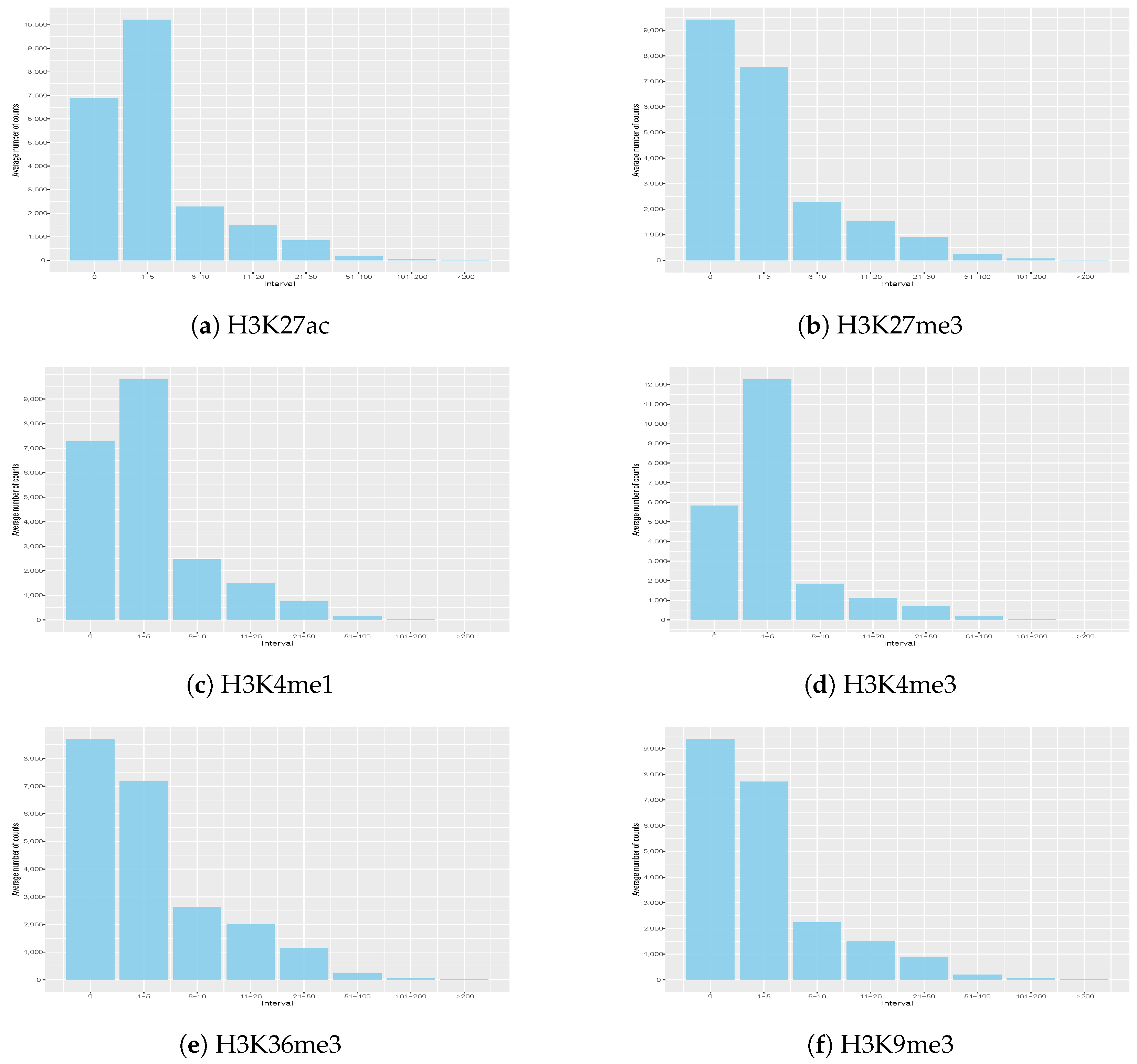
3.2. Histone Signal Distribution

The first step of the experiments is dedicated to the analysis of histone modification signals along the genome. As stated in Section 2.3, whole-genome profiles of cell types are built by quantifying the number of peaks for each gene in the histone modification signal. In this phase, we investigate the possibility that a (relatively) high signal intensity of a histone modification is registered only in a fraction of genes. This hypothesis arises from the observation that in gene expression profiles, most genes are either constantly expressed or not expressed at all [27,28]. Consequently, if whole-genome histone modification profiles follow this behaviour, classical differential expression analysis techniques could be borrowed for processing histone signals.

We experimentally verify this hypothesis by comparing the distribution of the number of peaks per gene (see Figure 3 for a graphical representation) of the profiles of different cell types for each histone modification with the expected distributions of gene expression counts derived from the literature [27,28]. Figure 3 highlights that, as happens in RNA-seq experiments, very low or no signal is registered for the large majority of genes. Indeed, the vast majority of genes have counts equal to 0 or lower than 5. Interestingly, this behaviour appears to be independent of the type of modification.

Therefore, observation of the signal distribution opens up the use of standard differential gene expression normalisation methods for processing histone modification marks. These methods, in turn, can be exploited to perform feature selection in the experiments. Following this idea, each cell type profile is normalised using CPM and RPKM normalisation. Experiments are conducted in the R environment [19] by using the R functions cpm and rpkm from the edgeR package. Subsequently, a feature selection procedure is performed following the strategy described in Section 2.3. Feature selection is applied to both normalisations of the data, with the effect of retaining (i) genes with a consistent number of peaks and (ii) genes with well-differentiated values across samples. In

Table 2. The number of genes retained after feature selection using CPM and RPKM normalisation, respectively. In the last column, the number of genes retained by both normalisation methods are reported, showing that almost all the genes retained by RPKM are also maintained by CPM.

Modification	CPM	RPKM	INTERSECTION
H3K27ac	5655	481	340
H3K27me3	5294	235	184
H3K36me3	6062	369	264
H3K4me1	7309	248	206
H3K4me3	5627	235	189
H3K9me3	5295	383	280

, the number of features (genes) retained after feature selection is reported. Table 2 shows that out of 21,987 quantified genes, only a fraction are active. In particular, by using RPKM, thus requiring the signal intensity to be proportional to the gene length, the number of active genes is rather small (independent of the histone modification mark). Moreover, RPKM filters many more genes than CPM. This result suggests that there are a number of long genes with enough histone modification marks to be retained after CPM, but with a sufficient concentration of marks to also be retained after RPKM. Finally, by inspecting the number of genes retained after the application of both normalisation methods (see the last column of Table 2), we observe that few genes are retained after RPKM and filtered out by CPM. This suggests that such genes have small peaks, which emerge because of their short length.

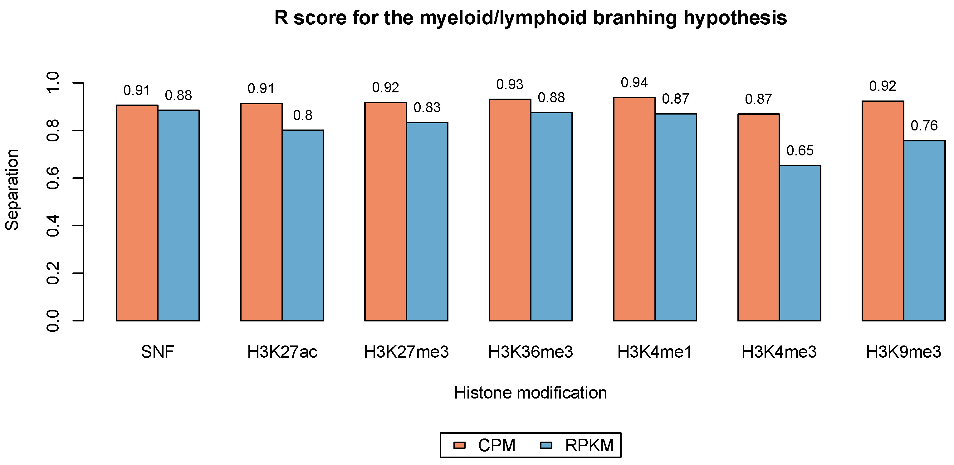
3.3. Phenotype Separation Evaluation

In view of evaluating the network integration and the hypothesis testing scheme presented in Section 2.4 and Section 2.5, the profiles from the six histone modifications are used to define similarity networks among cell types. The similarity measure is defined as in [14]. Then, the six resulting similarity networks are integrated into a unique graph using Similarity Network Fusion [14] (SNF). The application of SNF requires three parameters: K, T and $\mu$. K denotes the number of neighbours to consider in the K-Nearest Neighbours algorithm exploited by SNF, T is the number of iteration of the Cross Diffusion Process, and $\mu$ is a scaling parameter used in the iterative computation of the similarity matrices. In our experiments, we set their values to 5, 10 and 0.3, respectively.

Subsequently, the six similarity networks (corresponding to the six histone modifications analysed) and the results from SNF are turned into dissimilarity networks to test the hypothesis evaluation model described in Section 2.5. For the single-modification networks, edges between cell types are weighted with the normalised squared Euclidean distance between pairs of cell types (in the range $[0,1]$). For the network resulting from fusion, dissimilarities are computed as follows: First, the Z-score of each similarity weight is computed. Then, the Z-scores are inverted with respect to the mean to obtain a dissimilarity weight.

We choose to test the model for evaluating the separation of each graph into two subgroups of cell types belonging to two distinct lineages in the classic haematopoietic tree [15]. Figure 2 shows a simplified representation of a classical scheme of haematopoiesis, which imposes a strict binary distinction between the myeloid and lymphoid lineages at the first differentiation step. However, recent studies [29,30] have highlighted that this model is a simplification of the real haematopoietic process. Indeed, they admit the existence of some mechanisms allowing myeloid progenitor cells to differentiate into cells belonging to the lymphoid component and vice versa. Consequently, it is interesting to exploit our hypothesis testing model for quantitatively evaluating the separation of the networks of cell types into the components induced by the two lineages.

If the graphical model fits the hypothesis, a cut separating myeloid and lymphoid cell types in each dissimilarity graph would tend to mostly remove edges with a high dissimilarity score. If we allow the possibility that some lower-weighted edges can also be removed, the separation score is expected to be close to (but less than) 1.

Indeed, the results depicted in Figure 4 report a score near 1 for all the networks. In addition, Figure 4 shows that scores obtained using CPM-based normalisation are higher than those obtained using RPKM, even if the gap is not remarkable. This suggests that in order to trigger a certain phenotype, histone modification signals do not have to be spread uniformly along a gene, but it is enough to have them in sufficient concentration. However, although the scores are high, there is still margin to believe that the model shown in Figure 2 may not be the only mechanism describing haematopoiesis.

Finally, from the results of the single-histone modification networks (Figure 4), it emerges that the six histone modifications almost equally contribute to the haematopoietic branch at the first level. This result is enforced by the high score obtained in the SNF network.

4. Discussion

Histone modifications are complex signals that are not yet fully understood. It is known that an increase/decrease in the concentration of such signals has an impact on gene expression. Furthermore, we know that the presence of large peaks in the signal wave is associated with loci involved in a histone modification [16]. In our experiments, the possibility of using high-resolution peaks to quantify per-gene histone modifications was investigated. In this framework, we studied the distribution of high-resolution peaks across the genome, showing that they behave similarly to gene expression profiles. More specifically, it can be observed, analogous to what happens for gene expression, that only a small fraction of genes have a significant signal intensity. Following this idea, we normalised the histone modification profiles of cells by using CPM and RPKM normalisations. Both methods were tested on our data since the use of a specific normalisation requires different interpretation of signal behaviour. Indeed, CPM measures signal concentration. Accordingly, differences in phenotypes are activated with a sufficient change in the amount of signal in a gene, regardless of the signal distribution. This is consistent with the idea that histone modifications merely have the role of starting/stopping transcription. On the contrary, RPKM is a measure of signal distribution. It is based on the assumption that a significant change in the phenotype is triggered only when a high quantification of the signal is uniformly spread along the genome. In this case, histone modifications would have the role of making the entire gene sequence accessible/hidden to facilitate/prevent transcription.

The results reported in Figure 3 and Table 2 show that, similar to gene expression, in most cases the signal (the number of peaks) is almost absent. This is especially evident using RPKM normalisation. Indeed, after feature selection only a few genes are retained. This indicates the presence of long genes having a high enough number of peaks to pass the filtering threshold for CPM but not RPKM. However, as the intersections of the genes retained with CPM and RPKM show, the opposite phenomenon is also present. In fact, there are short genes whose peak concentration is not sufficient to pass CPM filtering but that have signal distribution exceeding that of RPKM. A further inspection of Table 2 also reveals that the number of active genes is quite constant for all the histone modification types. Although further investigation is required for a correct biological interpretation of this result, no histone modification signal appears to play a dominant role in the regulation of gene expression. Accordingly, the displayed phenotype comes from the combination of the single modifications. As an example, in the imprinted genes, both the H3K4me3 open chromatin mark and the H3K9me3 compact chromatin mark are present at the promoter site [31].

Based on this observation, we used the SNF method [14] to integrate all the histone modification signals into a unified similarity network among phenotypes. The resulting network, shown in Figure 5, is a graph in which the nodes correspond to cell types and edges are weighted with a similarity score between pairs of cell types. Edge thickness is proportional to the similarity score between connected cell types, so that thicker edges connect cells with similar profiles. The similarity networks of the single histone modifications can be found in the Supplementary Material (Figures S1–S6). Supplementary Material are numbered according to the order in which the modifications are reported in Table 2. All the networks are plotted with the Gephi software [32] using the ForceAtlas2 visualisation algorithm [32]. From observation of the single-modification networks and the fused network, it emerges that strong and common links are promoted by similarity network fusion, as expected. As an example, in Figure 5 cells of the innate immune system (neutrophils, monocytes, macrophages, eosinophils) are tightly linked. This is coherent with the presence of strong links (high similarity scores) among those cells in most of the single modification networks. Another observation regards the strong link in Figure 5 between the “endothelial cell of umbilical vein (proliferating)” and “effector memory CD8-positive, alpha-beta T cell”. The similarity score between these two cell types is not very high in the single-modification networks (it is slightly higher in Supplementary Figure S4, representing H3K4me1), but it has a similar value in all the networks. This common link is therefore enhanced by the fusion procedure. Overall, the fused network is a good representation of the combination of the single networks, thus giving an overview of the simultaneous effect of histone modifications in haematopoietic cell differentiation.

The SNF network and the similarity networks of the single histone modifications are exploited for the application of the proposed hypothesis testing model. In order to apply this model, the similarity scores were turned into dissimilarities. The hypothesis testing scheme was then applied to the resulting networks for testing a hypothesis on the biological process of haematopoiesis. More specifically, we evaluated the separation induced on the graphs by differentiation into myeloid and lymphoid lineages, i.e., the first split in the classical haematopoietic tree (see Figure 2). In the ideal case, the cost of the graph cut that partitions the SNF network into the two groups corresponding to the two lineages should be maximum. Indeed, the weights of edges between cell types of the same lineage should be stronger (equivalently, the dissimilarity score should be lower) than those between cell types of different lineages. The results reported in Figure 4 show that the partition separating myeloid and lymphoid cell types is nearly best-case. This indicates that the classic myeloid/lymphoid differentiation branching is a reasonable approximation of the haematopoietic process. However, the same results leave room for concluding that this model in not accurate enough to capture the complexity of haematopoiesis. Interestingly, by applying the hypothesis testing model to the single histone modification graphs, we found that all the signals approximate the classical model with comparable scores. This, once again, can be considered confirmation of the hypothesis that all histone modification marks cooperate for the development of the displayed phenotype.

Overall, the experiments have proven that histone modification marks can be quantified using high resolution peaks. This quantification behaves similarly to gene expression, with only a few genes containing a noticeable number of peaks. Moreover, the analysis of dissimilarity networks between 24 cell types belonging to the haematopoietic tree has shown a close relationship between a given phenotype and a profile of the modification marks. This opens for exploitation differential analysis tools to identify genes involved in a phenotype of interest.

5. Conclusions

Histone modifications are complex signals which regulate gene expression by modifying the three-dimensional structure of chromatin. By consequence, genes become more or less accessible for transcription. The complexity of these signals makes their mining very difficult.

In this paper, we have shown that high-resolution peak counting (down to a few bps) is a reasonable approach to build per-gene profiles of histone modification marks. Experimental analysis of the signals of six histone modifications belonging to 24 cell types highlights that these profiles follow a similar distribution to that of gene expression. The relevance of the peak-based analysis of histone profiles was validated by computationally assessing the classic lymphoid/myeloid differentiation at the first level of the haematopoietic tree. Indeed, our experiments confirm that the classic haematopoietic model fairly approximates the biological process, although suggesting that it does not completely capture its complexity.

In addition to the contribution on the specific topic of haematopoiesis, our work constitutes an advance in epigenetics by providing a framework for analysing histone modification data. Indeed, the signal distribution of histone modification profiles allows the use of standard differential expression techniques to identify genes whose modifications are involved in a given phenotype.

Finally, the proposed graph-based methodology can be easily applied to other application domains where hypotheses on the separation of a population into subgroups must be evaluated.

References

1. Hizume, K.; Yoshimura, S.H.; Takeyasu, K. Linker histone H1 per se can induce three-dimensional folding of chromatin fiber. Biochemistry 2005, 44, 12978–12989. [Google Scholar] [CrossRef] [PubMed]
2. Peterson, C.L.; Laniel, M.A. Histones and histone modifications. Curr. Biol. 2004, 14, R546–R551. [Google Scholar] [CrossRef] [PubMed] [Green Version]
3. Jenuwein, T.; Allis, C.D. Translating the histone code. Science 2001, 293, 1074–1080. [Google Scholar] [CrossRef] [PubMed] [Green Version]
4. Kimura, H. Histone modifications for human epigenome analysis. J. Hum. Genet. 2013, 58, 439–445. [Google Scholar] [CrossRef] [Green Version]
5. Karlić, R.; Chung, H.R.; Lasserre, J.; Vlahoviček, K.; Vingron, M. Histone modification levels are predictive for gene expression. Proc. Natl. Acad. Sci. USA 2010, 107, 2926–2931. [Google Scholar] [CrossRef] [Green Version]
6. Mardis, E.R. ChIP-seq: Welcome to the new frontier. Nat. Methods 2007, 4, 613–614. [Google Scholar] [CrossRef]
7. O’Geen, H.; Echipare, L.; Farnham, P.J. Using ChIP-seq technology to generate high-resolution profiles of histone modifications. In Epigenetics Protocols; Springer: Berlin/Heidelberg, Germany, 2011; pp. 265–286. [Google Scholar]
8. Bujold, D.; Morais, D.A.d.; Gauthier, C.; Côté, C.; Caron, M.; Kwan, T.; Chen, K.C.; Laperle, J.; Markovits, A.N.; Pastinen, T.; et al. The International Human Epigenome Consortium Data Portal. Cell Syst. 2016, 3, 496–499.E2. [Google Scholar] [CrossRef] [Green Version]
9. Lawrence, M.; Daujat, S.; Schneider, R. Lateral Thinking: How Histone Modifications Regulate Gene Expression. Trends Genet. 2016, 32, 42–56. [Google Scholar] [CrossRef] [Green Version]
10. Bannister, A.; Kouzarides, T. Regulation of chromatin by histone modifications. Cell Res. 2011, 21, 381–395. [Google Scholar] [CrossRef]
11. Pepke, S.; Wold, B.; Mortazavi, A. Computation for ChIP-seq and RNA-seq studies. Nat. Methods 2009, 6, S22–S32. [Google Scholar] [CrossRef]
12. Vaissière, T.; Sawan, C.; Herceg, Z. Epigenetic interplay between histone modifications and DNA methylation in gene silencing. Mutat. Res. Mutat. Res. 2008, 659, 40–48. [Google Scholar] [CrossRef] [PubMed]
13. Wang, B.; Jiang, J.; Wang, W.; Zhou, Z.H.; Tu, Z. Unsupervised metric fusion by cross diffusion. In Proceedings of the 2012 IEEE Conference on Computer Vision and Pattern Recognition, Providence, RI, USA, 16–21 June 2012; pp. 2997–3004. [Google Scholar] [CrossRef] [Green Version]
14. Wang, B.; Mezlini, A.; Demir, F.; Fiume, M.; Tu, Z.; Brudno, M.; Haibe-Kains, B.; Goldenberg, A. Similarity network fusion for aggregating data types on a genomic scale. Nat. Methods 2014, 11, 333–337. [Google Scholar] [CrossRef] [PubMed]
15. Prchal, J.T.; Throckmorton, D.W.; Carroll, A.J.; Fuson, E.W.; Gams, R.A.; Prchal, J.F. A common progenitor for human myeloid and lymphoid cells. Nature 1978, 274, 590–591. [Google Scholar] [CrossRef] [PubMed]
16. Blahnik, K.R.; Dou, L.; O’Geen, H.; McPhillips, T.; Xu, X.; Cao, A.R.; Iyengar, S.; Nicolet, C.M.; Ludäscher, B.; Korf, I.; et al. Sole-Search: An integrated analysis program for peak detection and functional annotation using ChIP–seq data. Nucleic Acids Res. 2010, 38, e13. [Google Scholar] [CrossRef] [PubMed] [Green Version]
17. Mortazavi, A.; Williams, B.A.; McCue, K.; Schaeffer, L.; Wold, B. Mapping and quantifying mammalian transcriptomes by RNA-Seq. Nat. Methods 2008, 5, 621. [Google Scholar] [CrossRef]
18. Lloyd, S. Least squares quantization in PCM. IEEE Trans. Inf. Theory 1982, 28, 129–137. [Google Scholar] [CrossRef] [Green Version]
19. R Core Team. R: A Language and Environment for Statistical Computing; R Foundation for Statistical Computing: Vienna, Austria, 2017. [Google Scholar]
20. Thorndike, R.L. Who belongs in the family? Psychometrika 1953, 18, 267–276. [Google Scholar] [CrossRef]
21. Tritchler, D.; Parkhomenko, E.; Beyene, J. Filtering genes for cluster and network analysis. BMC Bioinform. 2009, 10, 193. [Google Scholar] [CrossRef] [Green Version]
22. Karger, D.R. Global Min-cuts in RNC, and Other Ramifications of a Simple Min-Cut Algorithm. In Proceedings of the SODA, Austin, TX, USA, 25–27 January 1993; Volume 93, pp. 21–30. [Google Scholar]
23. Ford, L.R.; Fulkerson, D.R. Maximal flow through a network. Can. J. Math. 1956, 8, 399–404. [Google Scholar] [CrossRef]
24. Karp, R.M. Reducibility among combinatorial problems. In Complexity of Computer Computations; Springer: Berlin/Heidelberg, Germany, 1972; pp. 85–103. [Google Scholar]
25. Bansal, V.; Bafna, V. HapCUT: An efficient and accurate algorithm for the haplotype assembly problem. Bioinformatics 2008, 24, i153–i159. [Google Scholar] [CrossRef] [Green Version]
26. Stoer, M.; Wagner, F. A simple min-cut algorithm. J. ACM (JACM) 1997, 44, 585–591. [Google Scholar] [CrossRef]
27. Church, B.V.; Williams, H.T.; Mar, J.C. Investigating skewness to understand gene expression heterogeneity in large patient cohorts. BMC Bioinform. 2019, 20, 1–14. [Google Scholar] [CrossRef] [PubMed]
28. De Torrenté, L.; Zimmerman, S.; Suzuki, M.; Christopeit, M.; Greally, J.M.; Mar, J.C. The shape of gene expression distributions matter: How incorporating distribution shape improves the interpretation of cancer transcriptomic data. BMC Bioinform. 2020, 21, 562. [Google Scholar] [CrossRef] [PubMed]
29. Alberti-Servera, L.; von Muenchow, L.; Tsapogas, P.; Capoferri, G.; Eschbach, K.; Beisel, C.; Ceredig, R.; Ivanek, R.; Rolink, A. Single-cell RNA sequencing reveals developmental heterogeneity among early lymphoid progenitors. EMBO J. 2017, 36, 3619–3633. [Google Scholar] [CrossRef]
30. Perié, L.; Duffy, K.R.; Kok, L.; de Boer, R.J.; Schumacher, T.N. The branching point in erythro-myeloid differentiation. Cell 2015, 163, 1655–1662. [Google Scholar] [CrossRef] [Green Version]
31. Mikkelsen, T.S.; Ku, M.; Jaffe, D.B.; Issac, B.; Lieberman, E.; Giannoukos, G.; Alvarez, P.; Brockman, W.; Kim, T.K.; Koche, R.P.; et al. Genome-wide maps of chromatin state in pluripotent and lineage-committed cells. Nature 2007, 448, 553–560. [Google Scholar] [CrossRef]
32. Jacomy, M.; Venturini, T.; Heymann, S.; Bastian, M. ForceAtlas2, a continuous graph layout algorithm for handy network visualization designed for the Gephi software. PLoS ONE 2014, 9, e98679. [Google Scholar] [CrossRef]
Figure 1. Scheme of the proposed methodology. In Phase 1, histone modification profiles of cell types are built by counting peaks in the modification signal. In Phase 2, a similarity network of cell types is computed for each histone modification; the networks are then fused by using a similarity network [14]. In Phase 3, a graph-cut-based approach is introduced to evaluate the bipartition of the networks into myeloid and lymphoid cell types.
Mathematics 10 01842 g001
Figure 2. A simplified representation of the classical model of the haematopoietic tree, where the lymphoid and myeloid lineages are highlighted in blue and orange, respectively.
Mathematics 10 01842 g002
Figure 3. Distribution of the signal intensity of the histone modification profiles. The histograms show that most of the genes have no or poorly detectable signal intensity (i.e., lower than 10) while the signal is remarkably high only in a fraction of genes along each sample.
Mathematics 10 01842 g003
Figure 4. Barplot of the results of hypothesis testing for each modification network and for the network resulting from the fusion process (denoted SNF). The x-axis is labelled according to the different similarity networks. “SNF” refers to the network obtained after the fusion process. The y-axis contains the value of the separation score obtained after applying the graph cuts to the networks. For each network, the separation score is described by two coloured bars, distinguishing results obtained after CPM- or RPKM-based normalisation.
Mathematics 10 01842 g004
Figure 5. Similarity network of cell types obtained after applying the SNF method. Nodes are coloured according to the classical hypothesis on haematopoiesis: pink nodes correspond to cells labelled as “myeloid”; blue nodes correspond to cells labelled as “lymphoid”. Edge thickness is proportional to the similarity score between connected cell types.
Mathematics 10 01842 g005