An Output Feedback Controller for a Second-Order System Subject to Asymmetric Output Constraint Based on Lyapunov Function with Unlimited Domain

Abstract

In this work, a new robust controller is designed for a second-order plant model, considering asymmetric output constraints. The tracking error convergence and output constraint are achieved by using a control law whose output feedback term is user-defined and bounded: it takes on large but finite and user-defined values for tracking error values equal to or higher than the constraint boundary, and it comprises a previously known user-defined function for tracking error values far from the constraint boundary. This is a significant contribution that remedies two important limitations of common output constraint control designs: the infinite control effort for tracking error equal to or higher than the constraint boundary, and the impossibility of using previously known user-defined functions in the output feedback function for tracking error values far from the constraint boundary. As another contribution, the control design is based on the dead-zone Lyapunov function, which facilitates the achievement of convergence to a compact set with user-defined size, avoidance of discontinuous signals in the controller, and robustness to model uncertainty or disturbances. The proposed output feedback term consists of the product between two functions of the tracking error, an increasing function and a sigmoid function, whose exact expressions are user-defined. Finally, the effectiveness of the developed controller is illustrated by the simulation of substrate concentration tracking in a continuous flow stirred bioreactor.

1. Introduction

Many dynamic systems are subject to output constraint, which is related to performance requirements, physical limitations, or safety issues [1,2,3]. For instance, the joint position of robotic manipulators, and the velocity of nonholonomic and unmanned aerial vehicles should be limited [1,2,4].

In the control literature, a common strategy to tackle output constraint is the barrier Lyapunov function (BLF) [1], which was pioneered by [5]. Compared to other output constraint strategies, it has the advantage of easier implementation, as numerical or computationally intensive algorithms are avoided [4]. In the BLF strategy, the prescribed constant boundary defined for the tracking error is tackled through a Lyapunov function that involves a vertical asymptote at the prescribed boundary, so that it takes on large values for the tracking error values close to the boundary and it is not defined for tracking error values exceeding it. The output feedback term of the resulting control law also exhibits these features. Therefore, the achievement of output constraint within the prescribed boundaries is a consequence of the enhanced control effort [1,6,7]. Usually, the Lyapunov function is logarithm or tangent type [4], whereas sliding mode control (SMC) [4,6] or backstepping control [2,8] are used as basic control design framework. The main improvements to the basic BLF control design for higher-order nonlinear systems are the consideration of asymmetric constraint [1,2,3,4]; consideration of no strict feedback form systems [1,2,3]; use of finite-time stabilization [3,9].

An alternative way to achieve output constraint is by using a Lyapunov function defined over the whole domain of the tracking error, and a controller with output feedback terms featuring large but bounded values for the tracking error equal to the prescribed boundary [10]. Some control designs with these features (which we call FOC features) are discussed in what follows. In [10], a modification is proposed for the Lyapunov function used in traditional prescribed performance control (PPC). In [11], an output-constrained SMC is designed for systems of relative degree two involving disturbances. The first derivative of the output is constrained but not the output. The controller guarantees that the constraints can be violated during a finite time, which can be shortened by properly choosing the controller parameters. When there is a constraint violation event, the control law includes an additive term that is the function of the error between the constrained state and the constraint bound. The Lyapunov function used is a quadratic function of the sliding surface. In [12], a sliding mode control design with double power reaching law and variable power parameters is proposed. A changing magnitude of the parameters of the power terms of the reaching law is proposed, so as to improve the convergence rate of the approach phase. From the reaching law it follows that: (i) the control law involves a double power function of the sliding surface(s) with variable parameters; (ii) the gradient of the power function is higher when the sliding surface is farther from zero. As a result, the convergence speed of the sliding surface is faster for large values of the surface. Comparing the proposed SMC with the fast power reaching law, it achieves a faster convergence of the surface and a higher tracking precision in presence of time-varying disturbances. One deduces that this controller can be adapted to achieve output constraint requirements if the parameters of the double power function are chosen to fulfill the aforementioned FOC features.

In this work, a new robust controller is designed for the second-order plant model, considering asymmetric output constraints. The control design is based on dead-zone Lyapunov functions, aimed at achieving tracking error convergence. An improved output feedback term of the control law is proposed, consisting of the product between two user-defined functions of the tracking error: a basic increasing function and a sigmoid function that exhibits bounded but enhanced values for the tracking error equal to the constraint boundary. In this way, the output feedback term function is increasing with a steep section that leads to significantly higher but finite values for the tracking error equal to or higher than the constraint bound. The resulting control law yields an overlarge but bounded control effort for tracking error values equal to or higher than the prescribed constraint boundary. The main contributions over closely related output constraint control designs are:

−

Contribution Bi. The output feedback term of the control law, and consequently, the control law, take on large but finite and user-defined values when the tracking error values are equal to or higher than the prescribed constraint bound. In contrast, in BLF-based output constraint controllers (for instance [3,4,13]) the output feedback term, and consequently, the control law, give infinite values when the tracking error is equal to the constraint bound, and it is not defined for tracking error values higher than the constraint bound.

−

Contribution Bii. The output feedback term of the control law is equal to a user-defined output function when the tracking error is far from the constraint bound. This implies that high-performance output feedback functions, for instance, the well-known power-law functions, can be used in the controller for these tracking error values. In contrast, in BLF-based output constraint controllers (see [3,4,13]), previously known user-defined functions cannot be used in the output feedback term for tracking error values far from the constraint boundary.

−

Contribution Biii. The advantages of control design based on dead-zone Lyapunov functions are achieved, for instance, the absence of discontinuous signals in the controller whereas keeping robustness against disturbances or modeling error. In contrast, in BLF-based output constrain controllers (e.g., [4,13]), discontinuous signum type signals are used in the control law.

The system model, the reference model and the control goal are provided in Section 2, and the controller design and stability analysis in Section 3. The numerical simulation is provided in Section 4, and the conclusions are drawn in Section 5.

2. System Model, Reference Model and Control Goal

SISO second-order nonlinear model represent several systems, including mechatronic, biochemical and networked systems. This model usually includes disturbance terms caused by parametric uncertainty, modeling error, unmodeled parasitic dynamics and unknown external disturbances [14,15,16]. Consider a SISO second-order model with states $x_1$, $x_2$,:

$$\frac{d{x}_1}{dt}=F_1+F_{g1}{x}_2+{\delta }_1,$$

(1a)

$$\frac{d{x}_2}{dt}=F_2+b_{m}u+{\delta }_2.$$

(1b)

where $x_1$ is the state to be controlled and $u$ is the input. The model terms satisfy the following assumptions:

Assumption 1.

The state $x_2$is bounded for$u$bounded, $x_1\in ℝ$, $x_2\in ℝ$.

Assumption 2.

The state $x_1$is measured and $u$is known.

Assumption 3.

$F_1$, $F_2$and $F_{g1}$are known functions of $x_1$and $x_2$; and $b_m$is known; ${\delta }_1$, ${\delta }_2$are unknown but bounded terms, with unknown bounds.

Remark 1.

Assumption 1, that is, $x_2$is bounded if $u$bounded, is a case of input to state stability (ISS), which is commonly accomplished in practical scenario. Additionally, it implies that the nonlinear system can be globally stabilized in the presence of input saturation [17,18].

Remark 2.

Assumption 2 implies that the measurement of $x_1$must be accurate for the application of the proposed controller. Hence, cases with significant noise are not allowed.

Remark 3.

In Assumption 3, the bounded disturbance terms are caused by either parametric uncertainty, modeling error, unmodeled parasitic dynamics or unknown external disturbances [14,15,16]. Thus, these terms render the model more akin to practical scenario.

Remark 4.

As the state $x_2$is not required to be known in the assumptions, real-time measurement of $x_2$ is not needed. This unavailability of knowledge on some state is common in practical scenarios, due to either environmental disturbances, equipment cost or technical limitation [1].

The input $u$ is constrained and its relationship with the unconstrained input signal $u_{nc}$ is:

$$u=\{\begin{array}{c}{u}_{max} if u_{nc}>u_{max}\\ u_{nc} if u_{nc} \in \left[u_{min} u_{max}\right]\\ u_{min} if u_{nc}<u_{min} \end{array}$$

(2)

where $u_{min}$, $u_{max}$ are constant input constraints.

Remark 5.

The input saturation is due to limitations on physical structure of the actuator. Therefore, the input constraints$u_{min}$, $u_{max}$ are defined by operational limits [19].

An observer is considered in order to cope with the lack of knowledge on $x_2$ and to avoid the risk of excessive increase of updated parameters, what is caused by input saturation (2). The observer model can be represented as:

$$\frac{d{\widehat{x}}_1}{dt}=H_{ad1}+H_{g1} {\widehat{x}}_2$$

(3a)

$$\frac{d{\widehat{x}}_2}{dt}=H_{ad2}+b_{m}u$$

(3b)

where ${\widehat{x}}_1$ is the estimate of $x_1$; ${\widehat{x}}_2$ is the estimate of $x_2$; $H_{ad1}$, $H_{g1}$,$H_{ad2}$, $b_m$ are known functions of $x_1$ and $x_2$. The controller design in Section 3 uses this observer model instead of the system model (1).

Remark 6.

Observers of this form are commonly used, for instance [20]. Alsoan example of observer for model (1) is provided in Appendix A, based on [21].

Control goal. Consider the tracking error $e_1={\widehat{x}}_1-y_d$, where $y_d$ is desired output provided by the reference model

$$y_d=\frac{a_m}{p+a_m}\frac{a_m}{p+a_m}r$$

(4)

where $r$ is the reference signal, and $a_m$ is a user-defined positive constant, and p = d/dt is the differential operator [22,23]. The goal of the controller design is to formulate the control an update laws that achieve the convergence of the tracking error $e_1$ towards the compact set ${\mathsf{\Omega }}_{e1}=\left\{e_1: \left|e_1\right|\le \epsilon \right\}$, and the constraint of the tracking error $e_1$ within a region with upper bound ${\epsilon }_u$ or lower bound $-{\epsilon }_l$, as user-defined, by using a controller with an output feedback function that has the following features: (i) it exhibits large but bounded and user-defined values for tracking error equal to or higher than the prescribed constraint bound; (ii) it involves a previously known user-defined function for tracking error values far from the constraint bound; (iii) it is non-decreasing with the tracking error, but its exact expression is user-defined. The width of the target compact set $\epsilon$, the upper constraint bound ${\epsilon }_u$ and the lower constraint bound $-{\epsilon }_l$ are user-defined and constant, and $\epsilon$, ${\epsilon }_u$, ${\epsilon }_l$, are positive.

Remark 7.

The observer (3) is used in the controller design in order to cope with the lack of knowledge on the state$x_2$and the effect of input saturation (2). Thus, the observer model is used instead of the system model (1), and the estimates ${\widehat{x}}_1$, ${\widehat{x}}_2$ are used instead of$x_1$, $x_2$.

3. Control Algorithm, Controller Design and Stability Analysis

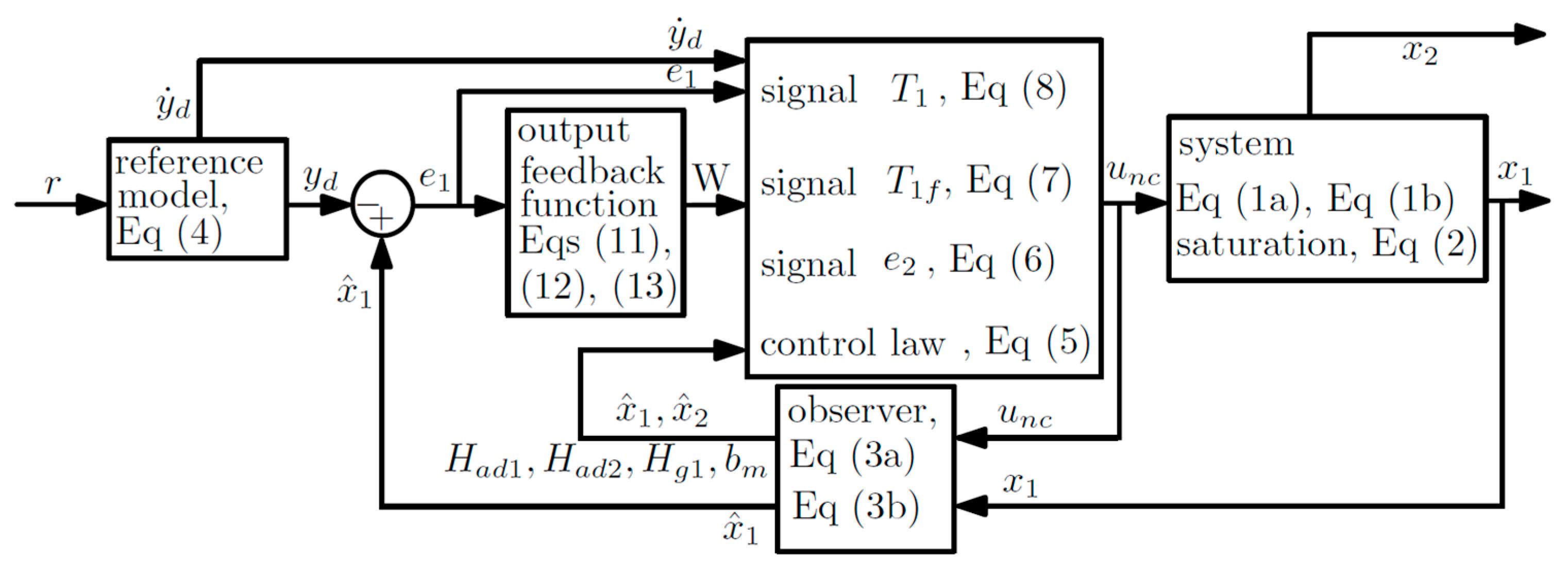
3.1. Control Algorithm

The controller is:

$$u_{nc}=\frac{1}{b_m}\left(-k_{c2}{H}_{g1}^2{e}_2-H_{ad2}-\frac{d{T}_{1f}}{dt}\right)$$

(5)

where

$$e_2={\widehat{x}}_2+T_{1f}$$

(6)

$T_{1f}$ is given by

$$\frac{d{T}_{1f}}{dt}=\frac{1}{{\tau }_{T1}}\left(-T_{1f}+T_1\right)$$

(7)

$${\mathrm{T}}_1=\frac{\left(W-{\dot{y}}_d\right)+H_{ad1}}{H_{g1}}+k_f{\mathrm{sat}}_{\mathrm{e}1}$$

(8)

$$sa{t}_{e1}=\{\begin{array}{c}\frac{e_1}{\epsilon }\left(2-\frac{\left|e_1\right|}{\epsilon }\right) for e_1\in \left(–\epsilon , \epsilon \right)\\ sgn\left(e_1\right) otherwise\end{array}$$

(9)

$$k_{c1}{k}_{c2}>\left(\frac{1}{4}\right); {\mathrm{k}}_{\mathrm{f}}\ge {\mu }_f+\epsilon >0$$

(10)

where $H_{ad1}$,$H_{ad2}$, $H_{g1}$ are functions of observer model (3), and: (i) ${\widehat{x}}_1$, ${\widehat{x}}_2$, are state estimates provided by the observer; (ii) $k_{c1}$, $k_{c2}$ are user-defined positive constants; (iii) ${\tau }_{T1}$ is the time constant of the signal $T_{1f}$; (iv) $k_f$ is the gain of the term for robustness against the error caused by the difference $T_1-T_{1f}$.

In addition,

$$W={\varphi }_a{f}_{ehc}$$

(11)

where $f_{ehc}$ is a function that leads to increased $W$ value for $e_1$ values equal to or higher than the constraint boundary:

$$\begin{array}{c}{f}_{ehc} \mathrm{is} \mathrm{continuous} \mathrm{and} \mathrm{increasing} \mathrm{with} \mathrm{respect} \mathrm{to} e_1;\hfill \\ f_{ehc}\approx 1 \mathrm{for} e_1 \mathrm{values} \mathrm{far} \mathrm{from} \mathrm{the} \mathrm{bound} \mathrm{but} \mathrm{not} \mathrm{exceeding} \mathrm{it}, \mathrm{with} \mathrm{the} \mathrm{bound} \mathrm{being} \mathrm{either} {\epsilon }_u \mathrm{or}-{\epsilon }_l; \hfill \\ f_{ehc}\gg 1 \mathrm{for} e_1 \mathrm{values} \mathrm{close} \mathrm{to} \mathrm{the} \mathrm{bound} ({\epsilon }_u or-{\epsilon }_l); \hfill \\ f_{ehc}\gg 1 \mathrm{for} e_1 \mathrm{values} \mathrm{exceeding} \mathrm{the} \mathrm{bound}, \mathrm{that} \mathrm{is}, e_1>{\epsilon }_u \mathrm{in} \mathrm{case} \mathrm{of} \mathrm{upper} \mathrm{bound} {\epsilon }_u, \mathrm{or} \mathrm{for} e_1<-{\epsilon }_l \mathrm{in} \mathrm{case} \mathrm{of} \mathrm{lower} \mathrm{bound}-{\epsilon }_l. \hfill \end{array}$$

(12)

and ${\varphi }_a$ is a previously known user-defined function of $f_{e1}$ that satisfies the properties:

$$\begin{gathered} {\varphi }_a=0 for f_{e1}=0 \\ {\varphi }_a\ne 0 for f_{e1}\ne 0 \\ sgn\left({\varphi }_a\right)=sgn\left(f_{e1}\right)\ne 0 for f_{e1}\ne 0 \\ {\varphi }_a \mathrm{is} \mathrm{continuous} \mathrm{with} \mathrm{respect} \mathrm{to} f_{e1} \\ {\varphi }_a \mathrm{is} \mathrm{non-decreasing} \mathrm{with} f_{e1} \end{gathered}$$

(13)

and

$$f_{e1}=\{\begin{array}{c}{e}_1-\epsilon for e_1\ge \epsilon \\ 0 for e_1 \in \left(-\epsilon , \epsilon \right)\\ e_1+\epsilon for e_1\le -\epsilon \end{array}$$

(14)

The block diagram of the controller is shown in Figure 1.

Remark 8.

The output feedback function $W$ (11) is a nonlinear function of the tracking error, and it exhibits the features mentioned in the control goal (Section 2):

−

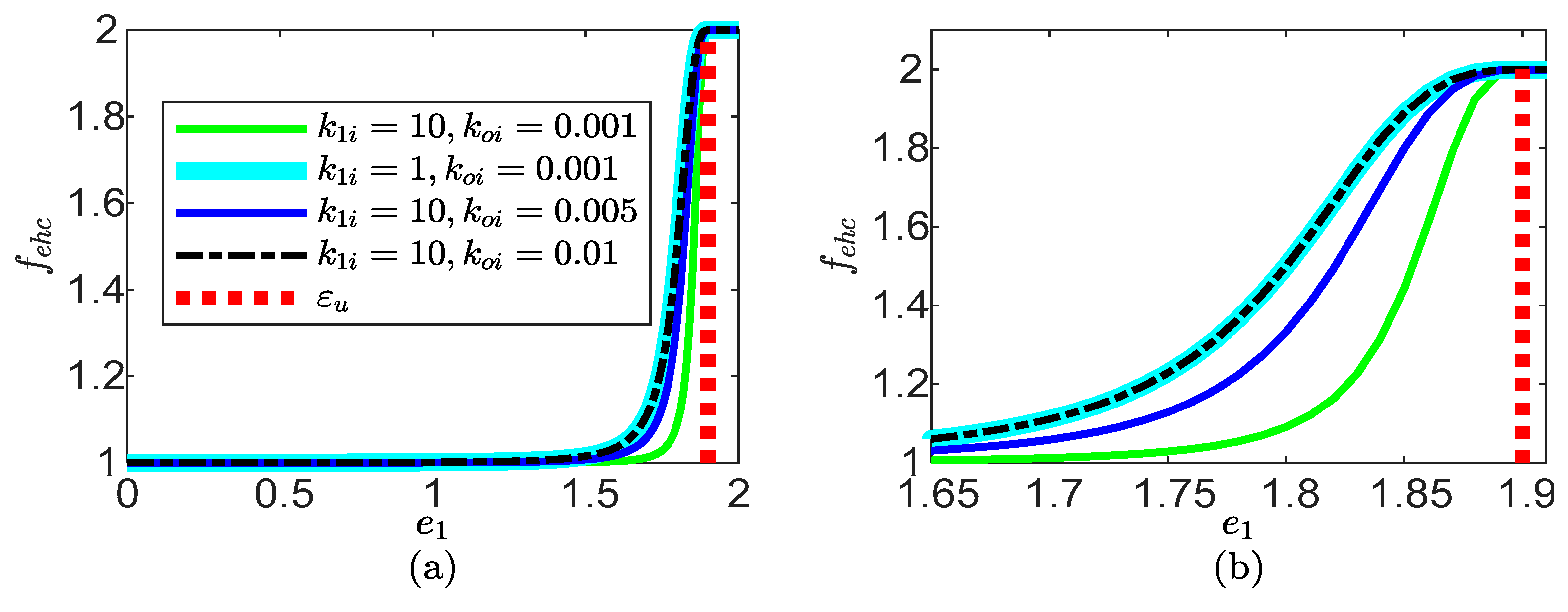
Bi: it takes on large but bounded and user-defined values for tracking error close, equal, or higher than the prescribed constraint boundary. It is achieved by using the sigmoid function $f_{ehc}$. This feature allows to achieve tracking error constraint.

−

Bii: it involves a previously known user-defined function ${\varphi }_a$ for tracking error values far from the constraint bound, but it must satisfy conditions (13).

Remark 9.

Functions ${\varphi }_a$ and $f_{ehc}$ must satisfy conditions (13) and (12), respectively, but their exact expressions are user-defined.

Remark 10.

An example of $f_{ehc}$ for the case of upper constraint boundary ${\epsilon }_u$ and no lower constraint is:

$$f_{ehc}=\left(1-f_T\right)\left(k_w-1\right)+1$$

(15)

$$f_T=\frac{k_{1i}{d}_{ct}^n}{k_{oi}+k_{1i}{d}_{ct}^n}, d_{ct}=\{\begin{array}{c}\left|{\epsilon }_u-e_1\right| for e_1\le {\epsilon }_u \\ 0 for e_1>{\epsilon }_u \end{array}, k_w>1$$

(16)

where $k_w$ is a user-defined positive constant that specifies the enhancement of $W$ for $e_1$ values close to the bound ${\epsilon }_u$, and $k_{oi}$, $k_{1i}$, $n$ are user-defined positive constants. The main features of $f_{ehc}$ (15) and $f_T$ (16) are:

$$\begin{gathered} f_T=0 for e_1\ge {\epsilon }_u \\ {f}_T\approx 1 for e_1\ll {\epsilon }_u \\ {f}_{ehc}=k_w for e_1\ge {\epsilon }_u \\ {f}_{ehc}\approx 1 for e_1 \ll {\epsilon }_u \end{gathered}$$

so that $f_{ehc}$ fulfills conditions (12).

Remark 11.

An example of ${\varphi }_a$ is

$${\varphi }_a=k_{\varphi 1}{\left|f_{e1}\right|}^{\alpha }sgn\left(f_{e1}\right)+k_{\varphi 2}{\left|f_{e1}\right|}^{3}sgn\left(f_{e1}\right)$$

(17)

which is based on the output feedback function used in [12,24]:

$${\varphi }_w=k_1{|●|}^{\alpha }sgn(●)+k_2{|●|}^{\beta }sgn(●)$$

(18)

where $\alpha >0$, $\beta >0$, $k_1>0$, $k_2>0$, and the ranges and values $\alpha \in \left[0.75, 1.6\right]$, $\beta \in \left[0.75, 1.6\right]$, $k_1=1.5$, $k_2=0.8$ were used in [12], whereas $\alpha =5/8$, $\beta =3$, $k_1=2.5\times 42.4$, $k_2=25\times 42.4$, were used in [24].

Remark 12.

In BLF based output constraint control, the Lyapunov function of the type

$$V_{e1}=\frac{{\epsilon }_u^{\alpha }}{\alpha }\frac{{\left|e_1\right|}^{\alpha }}{{\left({\epsilon }_u-e_1\right)}^{\alpha }}$$

with $\alpha \ge 2$ is commonly used, being ${\epsilon }_u$ the upper constraint [3,4,13]. The gradient of $V_{e1}$ is:

$$\frac{d{V}_{e1}}{d{e}_1}={\epsilon }_u^{\alpha +1}sgn\left(e_1\right)\frac{{\left|e_1\right|}^{\alpha -1}}{{\left({\epsilon }_u-e_1\right)}^{\alpha +1}}$$

Therefore, the resulting output feedback function of the control law involves the term $1/{\left({\epsilon }_u-e_1\right)}^{\alpha }$, which leads to infinite control effort for $e_1={\epsilon }_u$. A dead-zone modification can be incorporated in order to avoid discontinuous signals in the controller:

$$V_{e1}=\frac{{\epsilon }_u^{\alpha }}{\alpha }\frac{{\left|f_{e1}\right|}^{\alpha }}{{\left({\epsilon }_u-f_{e1}\right)}^{\alpha }}$$

$$\frac{d{V}_{e1}}{d{e}_1}={\epsilon }_u^{\alpha +1}sgn\left(f_{e1}\right)\frac{{\left|f_{e1}\right|}^{\alpha -1}}{{\left({\epsilon }_u-f_{e1}\right)}^{\alpha +1}}$$

A BLF-based output constraint controller comprises Equations (5)–(10), (14) with the above gradient $W=d{V}_{e1}/d{e}_1$, instead of the gradient (11)–(13). This allows to compare the proposed controller with respect to BLF-based output-constraint controller.

Remark 13.

The developed controller can be applied to second-order systems subject to output constraint, for instance mechatronic, mechanical and biochemical systems [14,15,16]. Indeed, output constraint is common in practical scenarios, and it is caused by physical limitations [6,25].

3.2. Controller Design and Stability Analysis

Theorem 1. 

Consider the desired output$y_d$provided by the reference model (4), the second order model (1) subject to assumptions 1–3, the observer (3), the tracking error $e_1={\widehat{x}}_1-y_d$, which isconstrained withina region with upper bound ${\epsilon }_u$ or lower bound $-{\epsilon }_l$, as user-defined, the controller (5)–(14). Then, the tracking error $e_1$ converges asymptotically to ${\mathsf{\Omega }}_{e1}=\left\{e_1: \left|e_1\right|\le \epsilon \right\}$, where the bound$\epsilon$is user-defined, positive and constant; and $e_1$ is constrained withina region with upper boundor lower bound$-{\epsilon }_l$, as user-defined.

Proof. 

Task 1 [Definition of the tracking error ${\mathit{e}}_{\mathit{1}}$ and its time derivative]. Recall the observer (3). We define the tracking error as $e_1={\widehat{x}}_1-y_d$. Differentiating with respect to time, yields

$$\frac{d{e}_1}{dt}=\frac{d{\widehat{x}}_1}{dt}-\frac{d{y}_d}{dt}$$

Incorporating the $d{\widehat{x}}_1/dt$ expression (3a), yields:

$$\frac{d{e}_1}{dt}=H_{g1}{\widehat{x}}_2+H_{ad1}-{\dot{y}}_d$$

(19)

Task 2 [Definition of (${\mathit{V}}_{\mathit{e}\mathit{1}}$) the dead-zone subsystem Lyapunov function for the tracking error, its gradient, and its properties]. The control goal includes the achievement of output tracking and the formulation of a controller with an output feedback function satisfying the stated features, being the exact output feedback function defined by the user. Therefore, $V_{e1}$, the Lyapunov function of the tracking error $e_1$, is defined as an integral of its gradient $W$ and the $V_{e1}$ and $W$ properties are defined, but the exact $W$ expression is not. Thus, the properties of $V_{e1}$, are set as:

$$\begin{gathered} V_{e1}=0 for f_{e1}=0 \\ {V}_{e1}>0 for f_{e1}\ne 0 \\ {V}_{e1} \mathrm{is} \mathrm{continuous} \mathrm{with} \mathrm{respect} \mathrm{to} f_{e1}, \\ {V}_{e1}\mathrm{is} \mathrm{bounded} \mathrm{for} f_{e1} \mathrm{bounded} \\ {V}_{e1} \mathrm{is} \mathrm{non-decreasing} \mathrm{with} \left|f_{e1}\right| \end{gathered}$$

(20)

where

$$f_{e1}=\{\begin{array}{c}{e}_1-\epsilon for e_1\ge \epsilon \\ 0 for e_1 \in \left(-\epsilon , \epsilon \right)\\ e_1+\epsilon for e_1\le -\epsilon \end{array}$$

(21)

The main properties of $f_{e1}$ (21) are:

$$\begin{gathered} f_{e1}=0 for e_1 \in \left[-\epsilon ,\epsilon \right] \\ {f}_{e1}\ne 0 for e_1\notin \left[-\epsilon ,\epsilon \right] \\ sgn\left(f_{e1}\right)=sgn\left(e_1\right)\ne 0 for e_1\notin \left[-\epsilon ,\epsilon \right] \\ {f}_{e1}\in {ℒ}_{\infty } for e_1 \in {ℒ}_{\infty } \end{gathered}$$

Thus, the $V_{e1}$ properties (20) in terms of $f_{e1}$ lead to the properties in terms of $e_1$:

$$\begin{gathered} V_{e1}=0 for e_1 \in \left[-\epsilon , \epsilon \right] \\ {V}_{e1}>0 for e_1 \notin \left[-\epsilon , \epsilon \right] \\ {V}_{e1} \mathrm{is} \mathrm{continuous} \mathrm{with} \mathrm{respect} \mathrm{to} e_1, \mathrm{and} \mathrm{it} \mathrm{is} \mathrm{bounded} \mathrm{for} e_1 \mathrm{bounded} \\ {V}_{e1} \mathrm{is} \mathrm{non-decreasing} \mathrm{with} \mathrm{increasing} \left|e_1\right| \end{gathered}$$

In order to obtain convergence of $e_1$ to the compact set ${\mathsf{\Omega }}_{e1}$ and to facilitate its proof, we require the gradient

$$W\triangleq \frac{d{V}_{e1}}{d{f}_{e1}}$$

(22)

to fulfill the following properties:

$$\begin{gathered} W=0 for f_{e1}=0 \\ W\ne 0 for f_{e1}\ne 0 \\ sgn\left(W\right)=sgn\left(f_{e1}\right)\ne 0 for f_{e1}\ne 0 \\ W \mathrm{is} \mathrm{continuous} \mathrm{with} \mathrm{respect} \mathrm{to} f_{e1} \\ W \mathrm{is} \mathrm{non-decreasing} \mathrm{with} f_{e1} \end{gathered}$$

(23)

As a consequence, the properties of $W$ in terms of $e_1$ are:

$$\begin{gathered} W=0 for e_1 \in \left[-\epsilon , \epsilon \right] \\ W\ne 0 for e_1 \notin \left[-\epsilon , \epsilon \right] \\ sgn\left(W\right)=sgn\left(e_1\right)=sgn\left(f_{e1}\right)\ne 0 for e_1 \notin \left[-\epsilon , \epsilon \right] \\ W \mathrm{is} \mathrm{continuous} \mathrm{with} \mathrm{respect} \mathrm{to} e_1 \\ W \mathrm{is} \mathrm{non-decreasing} \mathrm{with} e_1 \end{gathered}$$

(24)

A practical way to define $V_{e1}$ and $W$ is to define a $W$ function of $f_{e1}$ that satisfies properties (23), and then to determine $V_{e1}$ from

$$V_{e1}={\int }_0^{f_{e1}} Wd{f}_{e1}$$

What leads to fulfillment of $V_{e1}$ properties (20). The integral form of $V_{e1}$ for the case of asymmetrical is considered in Appendix B. The basic choice of $W$ is $W=k_{c1}{f}_{e1}$ which fulfills properties (23) and leads to $V_{e1}=\left(1/2\right)k_{c1}{f}_{e1}^2$, which fulfills properties (20).

Task 3 [Determination of$d{V}_{e1}/dt$and incorporation of the output feedback term]. The time derivative of $V_{e1}$ can be expressed as

$$\frac{d{V}_{e1}}{dt}=\frac{d{V}_{e1}}{d{e}_1}\frac{d{e}_1}{dt}$$

(25)

From the definition of $W$ (22), the definition of $f_{e1}$ (21) and the properties of $W$ (24), it follows that

$$\frac{d{V}_{e1}}{d{e}_1}=W$$

Combining with Equation (25), yields

$$\frac{d{V}_{e1}}{dt}=W\frac{d{e}_1}{dt}$$

Incorporating the $d{e}_1/dt$ expression (19), yields

$$\frac{d{V}_{e1}}{dt}=-W^2+W\left(H_{g1}{\widehat{x}}_2+\left(W-{\dot{y}}_d\right)+H_{ad1}\right)$$

(26)

where the term $W^2$ has been subtracted and added to provide the non-positive term $-W^2$ in the $d{V}_{e1}/dt$ expression, what allows obtaining convergence of $e_1$ towards the expected compact set.

Task 4 [Definition of the second backstepping state$e_2$]. Equation (26) can be rewritten as

$$\frac{d{V}_{e1}}{dt}\le -W^2-k_f{H}_{g1}\left|W\right|+W{H}_{g1}\left({\widehat{x}}_2+\frac{\left(W-{\dot{y}}_d\right)+H_{ad1}}{H_{g1}}+k_{f}sign\left(W\right)\right)$$

(27)

where the term $-k_f{H}_{g1}\left|W\right|$ has been added and subtracted to provide robustness against an error term that will arise later because of the filtering approximation. To avoid the discontinuous signal $sign\left(f_{e1}\right)$, we notice from the W properties (24) that:

$$\left|W\right|=Wsa{t}_{e1}$$

with

$$sa{t}_{e1}=\{\begin{array}{c}\frac{e_1}{\epsilon }\left(2-\frac{\left|e_1\right|}{\epsilon }\right) for e_1\in \left(–\epsilon , \epsilon \right)\\ sgn\left(e_1\right) otherwise\end{array}$$

$$\frac{dsa{t}_{e1}}{d{e}_1}=\{\begin{array}{c}\frac{2}{\epsilon }\left(1-\frac{\left|e_1\right|}{\epsilon }\right) for e_1\in \left(–\epsilon , \epsilon \right)\\ 0 otherwise\end{array}$$

Therefore, Equation (27) can be rewritten as

$$\frac{d{V}_{e1}}{dt}\le -W^2-k_f{H}_{g1}\left|W\right|+W{H}_{g1}\left({\widehat{x}}_2+\frac{\left(W-{\dot{y}}_d\right)+H_{ad1}}{H_{g1}}+k_{f}sa{t}_{e1}\right)$$

Or equivalently,

$$\frac{d{V}_{e1}}{dt}\le -W^2-k_f{H}_{g1}|W|+W{H}_{g1}\left({\hat{x}}_2+T_1\right)$$

(28)

where

$$T_1=\frac{\left(W-{\dot{y}}_d\right)+H_{ad1}}{H_{g1}}+k_f{\mathrm{sat}}_{\mathrm{e}1}$$

If $e_2$ were defined as $e_2={\hat{x}}_2+T_1$, the term dT₁/dt in its time derivative would involve an undesired ‘explosion of terms’. To avoid this effect, the DSC strategy involves the use of a filtered signal in the definition of $e_2$ [26,27]. Therefore, we propose a definition of $e_2$ with a filtered $T_1$, denoted as $T_{1f}$. Equation (28) can be rewritten as

$$\frac{d{V}_{e1}}{dt}\le -W^2-k_f{H}_{g1}\left|W\right|+W{H}_{g1}\left(e_2+{\delta }_{t1f}\right)$$

(29)

where

$$e_2={\widehat{x}}_2+T_{1f}$$

(30)

and $T_{1f}$ is given by

$$\frac{d{T}_{1f}}{dt}=\frac{1}{{\tau }_{T1}}\left(-T_{1f}+T_1\right)$$

(31)

and ${\delta }_{t1f}=T_1-T_{1f}$ is the error caused by filtering. In the current DSC strategy, it is assumed that the time derivative of the input signal of the filter is bounded, see [26]. In the case of filter given in Equation (31), that assumption would be $d{T}_1/dt \in L_{\infty }$. Equation (31) and $T_1\in {ℒ}_{\infty }$ imply $T_{1f}\in {ℒ}_{\infty }$ and, consequently, ${\delta }_{t1f}\in {ℒ}_{\infty }$, so that ${\delta }_{t1f}\le {\mu }_f$, where ${\mu }_f$ is a positive constant. Therefore, Equation (29) can be rewritten as:

$$\frac{d{V}_{e1}}{dt}\le -k_f{H}_{g1}\left|W\right|+{\mu }_f\left|H_{g1}\right|\left|W\right|-W^2+W{H}_{g1}{e}_2$$

(32)

If $k_f$ is chosen such that $k_f\ge {\mu }_f>0$, then $-k_f\left|H_{g1}\right|\left|W\right|+{\mu }_f\left|H_{g1}\right|\left|W\right|\le 0$, so that Equation (32) leads to

$$\frac{d{V}_{e1}}{dt}\le -W^2+W{H}_{g1}{e}_2$$

Task 5 [Determination of the time derivative$\mathit{d}{\mathit{e}}_{\mathbf{2}}\mathbf{/}\mathit{d}\mathit{t}$]. Differentiating $e_2$ (Equation (30)) with respect to time, yields

$$\frac{d{e}_2}{dt}=\frac{d{\widehat{x}}_2}{dt}+\frac{d{T}_{1f}}{dt}$$

Substituting expression for $d{\widehat{x}}_2/dt$ (Equation (3b)), yields

$$\frac{d{e}_2}{dt}=H_{ad2}+b_{m}u+\frac{d{T}_{1f}}{dt}$$

(33)

where $d{T}_{1f}/dt$ is given by Equation (31).

Task 6 [Definition of${\mathit{V}}_{\mathit{e}\mathbf{2}}$, the dead-zone Lyapunov function for${\mathit{e}}_{\mathbf{2}}$, determination of its time derivative and formulation of the control law]. As we need to obtain the convergence of the state $e_2$ (30) to ${\mathsf{\Omega }}_{e2}=\left\{e_2: \left|e_2\right|\le \epsilon \right\}$, we choose $V_{e2}$, the dead-zone Lyapunov-like function for the state $e_2$ as

$$V_{e2}=\frac{1}{2}{f}_{e2}^2$$

(34)

where

$$f_{e2}=\{\begin{array}{c}{e}_2-\epsilon for e_2\ge \epsilon \\ 0 for e_2 \in \left(-\epsilon , \epsilon \right)\\ e_2+\epsilon for e_2\le -\epsilon \end{array}$$

(35)

The main properties of $V_{e2}$ are:

$$\begin{gathered} V_{e2}=0 for e_2 \in \left[-\epsilon , \epsilon \right] \\ {V}_{e2}>0 for e_2 \notin \left[-\epsilon , \epsilon \right] \\ {V}_{e2} \mathrm{is} \mathrm{continuous} \mathrm{with} \mathrm{respect} \mathrm{to} e_2, \\ {V}_{e2} \mathrm{is} \mathrm{bounded} \mathrm{for} e_2 \mathrm{bounded} \end{gathered}$$

Differentiating $V_{e2}$ (34) with respect to time, yields

$$\frac{d{V}_{e2}}{dt}=f_{e2}\frac{d{e}_2}{dt}$$

Incorporating the $d{e}_2/dt$ expression (Equation (33)), and arranging, yields

$$\frac{d{V}_{e2}}{dt}=-{\mathrm{k}}_{\mathrm{c}2}{ \mathrm{H}}_{\mathrm{g}1}^2{\mathrm{f}}_{\mathrm{e}2}{\mathrm{e}}_2+f_{e2}\left(k_{c2}{\mathrm{H}}_{\mathrm{g}1}^2{e}_2+H_{ad2}+b_{m}u+\frac{d{T}_{1f}}{dt}\right)$$

(36)

To counteract the effect of the term $f_{e2}\left(k_{c2}{\mathrm{H}}_{\mathrm{g}1}^2{e}_2+H_{ad2}+d{T}_{1f}/dt\right)$ we choose the control law for $u_{nc}$ as:

$$u_{nc}=\frac{1}{b_m}\left(-k_{c2}{H}_{g1}^2{e}_2-H_{ad2}-\frac{d{T}_{1f}}{dt}\right)$$

(37)

Considering moments of no input saturation $\left(u=u_{nc}\right)$, substituting (37) into Equation (36), yields

$$\frac{d{V}_{e2}}{dt}=-{\mathrm{k}}_{\mathrm{c}2}{ \mathrm{H}}_{\mathrm{g}1}^2{\mathrm{f}}_{\mathrm{e}2}{\mathrm{e}}_2$$

(38)

Task 7 [Determination of the$\mathit{d}{\mathit{V}}_{\mathit{e}\mathbf{1}}\mathbf{/}\mathit{d}\mathit{t}\mathbf{+}\mathit{d}{\mathit{V}}_{\mathit{e}\mathbf{2}}\mathbf{/}\mathit{d}\mathit{t}$expression under the formulated controller and arrangement in terms of a non-positive function of${\mathit{e}}_{\mathbf{1}}$]. Adding expressions for $d{V}_{e1}/dt$(32) and $d{V}_{e2}/dt$ (38), yields:

$$\frac{d{V}_{e1}}{dt}+\frac{d{V}_{e2}}{dt}\le -k_f{H}_{g1}\left|W\right|+{\mu }_f\left|H_{g1}\right|\left|W\right|-k_{c1}\left({\beta }_1+{\beta }_2\right)W^2+W{H}_{g1}{e}_2-{\mathrm{k}}_{\mathrm{c}2}{ \mathrm{H}}_{\mathrm{g}1}^2{\mathrm{f}}_{\mathrm{e}2}{\mathrm{e}}_2$$

(39)

where ${\beta }_1, {\beta }_2$ are positive constants that satisfy ${\beta }_1+{\beta }_2=1, {\beta }_1\in \left(0, 1\right), {\beta }_2\in \left(0, 1\right)$, and the term $W{H}_{g1}{e}_2$ exhibits no non-positive nature, so that it must be counteracted by the non-positive terms

$$-k_f\left|H_{g1}\right|\left|W\right|-k_{c1}\left({\beta }_1+{\beta }_2\right)W^2-{\mathrm{k}}_{\mathrm{c}2}{ \mathrm{H}}_{\mathrm{g}1}^2{\mathrm{f}}_{\mathrm{e}2}{\mathrm{e}}_2$$

To this end, $e_2$ is expressed in terms of $f_{e2}$ and the term $-k_f\left|H_{g1}\right|\left|W\right|+{\mu }_f\left|H_{g1}\right|\left|W\right|+W{H}_{g1}{e}_{2 }$ appearing in Equation (39) is arranged at what follows. From the definition of $f_{e2}$ (35) it follows that

$$f_{e2}=e_2+d_{e2}.$$

$$d_{e2}=\{\begin{array}{c}-\epsilon for e_2\ge \epsilon \\ -e_2 for e_2 \in \left(-\epsilon , \epsilon \right)\\ \epsilon for e_2\le -\epsilon \end{array}$$

Therefore,

$$e_2=f_{e2}-d_{e2}, \left|d_{e2}\right|\le \epsilon$$

In view of this expression, the term $W{H}_{g1}{e}_2$ can be rewritten as $W{H}_{g1}{e}_2=W{H}_{g1}{f}_{e2}+W{H}_{g1}\left(-d_{e2}\right)$. Hence, $W{H}_{g1}{e}_2\le W{H}_{g1}{f}_{e2}+\epsilon \left|W\right| \left|H_{g1}\right|$. Therefore, the term $-k_f\left|H_{g1}\right|\left|W\right|+{\mu }_f\left|H_{g1}\right|\left|W\right|+W{H}_{g1}{e}_2$ leads to

$$-k_f\left|H_{g1}\right|\left|W\right|+{\mu }_f\left|H_{g1}\right|\left|W\right|+W{H}_{g1}{e}_{2 }\le -\left(k_f-{\mu }_f-\epsilon \right)\left|H_{g1}\right|\left|W\right|+H_{g1}W{f}_{e2}$$

(40)

If $k_f$ is chosen such that $k_f\ge {\mu }_f+\epsilon \ge \epsilon >0$, then $-\left(k_f-{\mu }_f-\epsilon \right)\left|H_{g1}\right|\left|W\right|\le 0$, and, consequently, Equation (40) leads to $-k_f\left|H_{g1}\right|\left|W\right|+{\mu }_f\left|H_{g1}\right|\left|W\right|+W{H}_{g1}{e}_2\le H_{g1}W{f}_{e2}$. Combining this expression with Equation (41) leads to

$$\frac{d{V}_{e1}}{dt}+\frac{d{V}_{e2}}{dt}\le -k_{c1}\left({\beta }_1+{\beta }_2\right)W^2+H_{g1}W{f}_{e2}-k_{c2} H_{g1}^2{f}_{e2}{e}_2$$

(41)

Some properties of $f_{e2}$ (35) are:

$$\begin{gathered} sgn\left(f_{e2}\right)=sgn\left(e_2\right)\ne 0 for e_2\notin \left[-\epsilon ,\epsilon \right]; \\ \left| f_{e2}\right|<\left|e_2\right| for e_2 \notin \left[-\epsilon ,\epsilon \right]; f_{e2}=0 for e_2 \in \left[-\epsilon ,\epsilon \right] \end{gathered}$$

Hence,

$$\begin{gathered} e_2{f}_{e2}=\left|e_2\right| \left|f_{e2}\right|>f_{e2}^2 for e_2\notin \left[-\epsilon ,\epsilon \right] \\ {e}_2{f}_{e2}=0=f_{e2}^2 for e_2 \in \left[-\epsilon ,\epsilon \right] \end{gathered}$$

Combining these properties, yields $e_2{f}_{e2}\ge f_{e2}^2$. Therefore, $-k_{c2}{H}_{g1}^2{f}_{e2}{e}_2\le -k_{c2}{H}_{g1}^2{f}_{e2}^2$. Substituting this into Equation (41), yields

$$\frac{d{V}_{e1}}{dt}+\frac{d{V}_{e2}}{dt}\le -k_{c1}\left({\beta }_1+{\beta }_2\right)W^2+H_{g1}W{f}_{e2}-k_{c2}{H}_{g1}^2{f}_{e2}^2$$

(42)

where β₁ and β₂ are user-defined positive constants that satisfy ${\beta }_1+{\beta }_2=1, {\beta }_1\in \left(0, 1\right), {\beta }_2\in \left(0, 1\right)$. Equation (42) can be arranged as

$$\begin{gathered} \frac{d{V}_{e1}}{dt}+\frac{d{V}_{e2}}{dt}\le -k_{c1}{\beta }_1{W}^2 \\ +\left(-1\right)k_{c1}{\beta }_2\left[W^2+2W\left(\frac{1}{2k_{c1}{\beta }_2}{H}_{g1}{f}_{e2}\right)+4k_{c1}{k}_{c2}{\beta }_2{\left(\frac{H_{g1}{f}_{e2}}{2k_{c1}{\beta }_2}\right)}^2\right] \end{gathered}$$

(43)

If $k_{c1}$, $k_{c2}$ values are chosen such that $k_{c1}{k}_{c2}\ge \left(1/4\right){\beta }_2^{-1}$, then $4k_{c1}{k}_{c2}{\beta }_2\ge 1$ and Equation (43) lead to

$$\begin{gathered} \frac{d{V}_{e1}}{dt}+\frac{d{V}_{e2}}{dt}\le -k_{c1}{\beta }_1{W}^2+\left(-1\right)k_{c1}{\beta }_2{\left[W+\frac{1}{2k_{c1}{\beta }_2}{H}_{g1}{f}_{e2}\right]}^2 \\ \le -k_{c1}{\beta }_1{W}^2\le 0 \end{gathered}$$

(44)

Task 8. [Integration of the$d\left(V_{e1}+V_{e2}\right)V/dt$expression, and determination of the convergence of$e_1$]. Arranging and integrating Equation (44) yields

$$V_{e1}+V_{e2}+k_{c1}{\beta }_1{{\displaystyle \int }}_{to}^t{W}^{2}dt\le V_{e1|to}+V_{e2|to}$$

where $V_{e1|to}, V_{e2|to}$ are $V_{e1}$ (20), $V_{e2}$ (34) at time $to$. From the above expression it follows that $V_{e1}\le V_{e1|to}+V_{e2|to}$; $V_{e2}\le V_{e1|to}+V_{e2|to}$; $k_{c1}{\beta }_1{{\displaystyle \int }}_{to}^t{W}^{2}dt\le V_{e1|to}+V_{e2|to}$. Therefore, applying Barbalat’s lemma [28], we obtain the result that $f_{e1}$ converges asymptotically to zero, and the definition of $f_{e1}$ (21) implies that $e_1={\widehat{x}}_1-y_d$ converges asymptotically to ${\mathsf{\Omega }}_{e1}$, ${\mathsf{\Omega }}_{e1}=\left\{e_1: \left|e_1\right|\le \epsilon \right\}$, for moments of no input saturation. This completes the proof.

Task 9 [Definition of the structure of the output feedback term of the controller]. From the control law (37) it follows that the output feedback function $W$ has a straightforward effect on the control law. To achieve the output feedback function features stated in the control goal, we propose the output feedback function structure

$$W={\varphi }_a{f}_{ehc}$$

(45)

where $f_{ehc}$ is a function that increases the value of $W$ for $e_1$ values equal to or higher than the constraint bound (${\epsilon }_u or-{\epsilon }_l$):

• it is continuous and increasing with respect to $e_1$;
• $f_{ehc}\approx 1$ for $e_1$ values far from the bound, either ${\epsilon }_u$ or $-{\epsilon }_l$;
• $f_{ehc}\gg 1$ for $e_1$ values close to the bound (${\epsilon }_u or-{\epsilon }_l$);
• $f_{ehc}\gg 1$ for $e_1>{\epsilon }_u$ in case of upper bound ${\epsilon }_u$, or $e_1<-{\epsilon }_l$ in case of lower bound $-{\epsilon }_l$.

The function ${\varphi }_a$ is a previously known user-defined function of $f_{e1}$ that satisfies the W properties (23):

$$\begin{gathered} {\varphi }_a=0 for f_{e1}=0 \\ {\varphi }_a\ne 0 for f_{e1}\ne 0 \\ sgn\left({\varphi }_a\right)=sgn\left(f_{e1}\right)\ne 0 for f_{e1}\ne 0 \\ {\varphi }_a is continuous with respect to f_{e1} \\ {\varphi }_a is \mathit{non-decreasing} with f_{e1} \end{gathered}$$

(46)

Some examples of ${\varphi }_a$ and $f_{ehc}$ are given in Equations (15), (17) and (18). □

3.3. Discussion of Results

The developed controller design considers a second-order model with model uncertainties and output error constraints. Asymmetric tracking error constraint is considered. The main closed loop features are: (i) the tracking error converges to a compact set whose width is user-defined so that it depends on neither model terms, modeling error, nor model coefficients; (ii) output error constraint is achieved by using enhanced control effort; (iii) discontinuous signals are avoided in the controller. In addition, the output feedback term of the control law takes on large values for tracking error values close to the constraint boundary.

The overall steps of the control design are: (i) definition of the tracking error $e_1$ and its time derivative; (ii) definition of the dead-zone Lyapunov-like function for the tracking error ($V_{e1}$), its gradient and its properties; (iii) determination of the time derivative $d{V}_{e1}/dt$, and incorporation of the output feedback term; (iv) definition of the second backstepping state $e_2$; (v) determination of the time derivative $d{e}_2/dt$; (vi) definition of the dead-zone Lyapunov-like function for $e_2$ ($V_{e2}$), determination of its time derivative, and formulation of the control law; (vii) determination of the $d\left(V_{e1}+V_{e2}\right)/dt$ expression under the formulated controller; (viii) integration of the $d\left(V_{e1}+V_{e2}\right)/dt$ expression and determination of the boundedness of the closed-loop signals and convergence of $e_1$; (ix) definition of the structure of the output feedback term of the controller.

The control design procedure aims at rendering the time derivative of the overall Lyapunov function non-positive. The backstepping strategy is used as the basic framework for the control design, and the filtering approximation of the DSC strategy is used in order to avoid an ‘explosion of complexity’. However, several improvements are incorporated in the basic backstepping-DSC procedure to achieve contributions Bi, Bii and Biii: an additional robustness term is used in order to tackle the effect of the approximation error; dead-zone modification is used in the Lyapunov-like function; a new output feedback stabilizing term is incorporated in the time derivative $d{V}_{e1}/dt$.

The dead-zone modification of the Lyapunov functions has the following advantages: it allows for avoiding discontinuous signals in the controller signals, while robustness to disturbances or uncertainty terms is ensured; it facilitates guaranteeing the convergence of the tracking error to the user-defined region. Dead-zone Lyapunov functions have been mainly applied to robust control design: early studies are presented in [22,29,30], whereas recent studies in [31,32,33,34,35]. In turn, the theory of the dead-zone Lyapunov function keeps several of the advantages of the current Lyapunov function, including its usefulness for proving global asymptotic stability and for formulating nonlinear control which can be noticed in [36,37].

The output feedback function $W$ (45) is a nonlinear function of the tracking error, and it exhibits the advantages mentioned in the control goal (Section 2):

−

Bi: it takes on large but bounded and user-defined values for tracking error close, equal, or higher than the prescribed constraint bound, which is done through the sigmoid function $f_{ehc}$. This function satisfies conditions (12), whereas its exact expression and the level of enhancement $k_w$ are user-defined. The tracking error constraint is achieved through this control effort enhancement.

−

Bii: it involves a previously known user-defined output feedback function ${\varphi }_a$ for tracking error values far from the constraint bound. This function satisfies conditions (46), whereas its exact expression is user-defined so that high-performance functions are allowed, for instance the double power law (18).

4. Numerical Simulation

In this section, the controller and convergence results stated in Theorem 1 are illustrated through simulation for a continuous bioreactor, using the input constraint condition (2), the reference model (4) and the controller Equations (5)–(14). We consider a continuous culture of Gluconacetobacter diazotrophicus with constant culture volume and substrate sensor dynamics, being the measured substrate concentration ($s_s$) the output to be controlled and the dilution rate ($D$) the control input. Its model comprises biomass and substrate mass balance equations [20] and substrate sensor dynamics [38]:

$$\frac{d{s}_s}{dt}=-\frac{1}{{\tau }_1}{s}_s+\frac{1}{{\tau }_1}s$$

(46a)

$$\frac{ds}{dt}=\left(s_{in}-s\right)D-y_s\mu x$$

(46b)

$$\frac{dx}{dt}=\left(\mu -D\right)x$$

(46c)

where $x$ is the biomass concentration; $x_2=s$ is the substrate concentration; $s_{in}$ is the inlet substrate concentration; $\mu$ is the specific growth rate, $y_s$ is the yield coefficient; $y_s\mu$ is the substrate uptake rate, $D=Q/V$ is the dilution rate; $Q$ is the feeding flow rate; $V$ is the liquid volume [20] and $x_1=s_s$ is the output of the substrate sensor [38]. The equations for substrate measurement (46a) and substrate concentration (46b) correspond to model (1) and fulfill assumptions 1 to 3. The bacterium strain, initial medium composition, temperature, pH, dissolved oxygen concentration and mixing conditions correspond to the batch cultivation presented in [39]. The specific growth rate expression is

$$\mu ={\mu }_{max}{\left(1-\frac{x}{x_{max}}\right)}^f$$

The parameters of substrate and biomass models (46b), (46c) are fitted to batch culture data presented in [39], giving as result: ${\mu }_{max}=0.01484$ h-1; $X_{max}=0.32$ g/L; $f=1.607$; $y_s=0.0234$; $m_s=0.22425$. In addition, $s_{in}=180$ g/L and ${\tau }_1=0.03$ h were used for the continuous plant models (46). The width of the tracking error convergence set ${\mathsf{\Omega }}_{e1}$, the constraint boundary and the input bound are set to $\epsilon =1.3$; ${\epsilon }_u=1.9$; $D_{max}=4$. The observer used is based on that of [20], and the state estimation results in ${\widehat{x}}_1\approx x_1$, and ${\widehat{x}}_2\approx x_2$.

The parameters of control Equations (5)–(11) are chosen as $a_m=0.1$; ${\tau }_{T1}=0.01$; $k_f=0.195$. We use an asymmetric form of (17) for ${\varphi }_a$:

$${\varphi }_a=\{\begin{array}{c}{k}_{\varphi 1}{\left|f_{e1}\right|}^{\alpha }sgn\left(f_{e1}\right)+k_{\varphi 2}{\left|f_{e1}\right|}^{3}sgn\left(f_{e1}\right) for e_1>0\\ -k_{c1}{f}_{e1} for e_1\le 0\end{array}$$

with $k_{c1}=0.5$; $k_{\varphi 1}=0.0002164$; $k_{\varphi 2}=4.408$; $\alpha =1.417$, so that the $W$ function is:

$$W=\{\begin{array}{c}{\varphi }_a{f}_{ehc} for e_1>0\\ -k_{c1}{f}_{e1} for e_1\le 0\end{array}$$

The function (15) is used for $f_{ehc}$: the effect of $k_{oi}$, $k_{1i}$, $n$ on the $f_T$ curve is shown in Figure 2, whereas their effect on the $f_{ehc}$ and $W$ curves is shown in Figure 3. The $f_T$ curve (Figure 2) shows that: the $f_T$ function is continuous and smooth; $f_T\approx 0$ for low $d_{ct}$ values; $f_T\approx 1$ for high values. In addition, steeper curve is obtained with high $n$, high k_1i, low $k_{oi}$.

The $f_{ehc}$ curve (Figure 3a,b) shows that: the $f_{ehc}$ function is continuous and smooth; $f_{ehc}\approx 1$ for low $e_1$ values; $f_{ehc}\approx k_w$ for $e_1$ close to ε_u. In addition, steeper form is obtained with high $n$, high $k_{1i}$, low $k_{oi}$.

The $W$ curve (Figure 3c,d) shows that: the $W$ function is continuous and smooth; $W\approx {\varphi }_a$ for low $e_1$ values; $W\approx k_w{\varphi }_a$ for $e_1$ close to ${\epsilon }_u$. In summary, the definition of $f_{ehc}$ parameters to obtain the desired $W$ features is simple, while involving the user-defined dependence for low $e_1$ values and for $e_1$ close to ε_u.

The values of $f_{ehc}$ are chosen to be $k_{oi}=0.001$, 10, $n=3$. The simulation is performed using MATLAB version R2014 with ode45 function. The trajectories of the tracking error $e_1$, the backstepping state $e_2$, the control input $D$, the output x₁ = S and the desired output $y_d$ for these $n$, $k_{oi}$, $k_{1i}$ values and different values of $e_{to}$ are shown in Figure 4 and Figure 5.

Simulations (Figure 4 and Figure 5) verify that:

−

the developed controller achieves a fast asymptotic convergence of the tracking error $e_1$ to the compact set ${\mathsf{\Omega }}_{e1}=\left\{e_1: \left|e_1\right|\le \epsilon \right\}$.

−

the dependence of the control effort on the tracking error is remarkably enhanced with the applied $f_{ehc}$ function (Figure 3 and Figure 4), thus avoiding violation of output constraint. This is mostly noticed at initial time when the tracking error is high and outside ${\mathsf{\Omega }}_{e1}$.

5. Conclusions

In this paper, we proposed a robust controller for systems described by the second-order input-output model, considering asymmetric tracking error constraints. The main contribution over closely related studies is that the tracking error convergence is achieved by using a control law whose output feedback term is user-defined and bounded, comprising large but finite user-defined values for tracking error values equal to or higher than the constraint boundary, and a user-defined function for tracking error values far from the constraint boundary. This is a significant contribution that remedies two important limitations of common output constraint control designs: the infinite control effort for tracking error equal to or higher than the constraint boundary, and the impossibility of using previously known user-defined functions in the output feedback function for tracking error values far from the constraint boundary. As another contribution, the control design is based on the dead-zone Lyapunov function, which facilitates the achievement of convergence to a compact set with user-defined size, avoidance of discontinuous signals in the controller and robustness to model uncertainty or disturbances.

To achieve the aforementioned features, the main improvements made in the control design procedure are: (i) dead zone modification is used in the Lyapunov function; (ii) the Lyapunov function for the tracking error is defined as an integral in terms of its gradient; (iii) the non-positive stabilizing term in the time derivative of the overall Lyapunov function is chosen to be the square of the output feedback term; (iv) the output feedback term is defined as the product between a sigmoid function and an increasing function, both of them depending on the tracking error.

The main limitations of the proposed controller are:

−

The design is only valid for the second-order systems, so that systems of higher-order are not allowed.

−

Finite-time stabilization is not guaranteed. That is, the time for convergence of the tracking error $e_1$ to its compact set ${\mathsf{\Omega }}_{e1}$ is not straightforwardly defined by the user. Indeed, some trial-and-error effort is needed for achieving a desired convergence time.

−

The control gain $b_m$ is considered completely known.

The simulations show several of the advantages mentioned in the contributions including (i) convergence of the tracking error to a compact set whose width is user-defined; (ii) the tracking error is constrained by using the proposed output feedback term in the control law; (iii) the input signal is continuous.

References

- Mei, K.; Ding, S. Output-feedback finite-time stabilization of a class of constrained planar systems. Appl. Math. Comput. 2022, 412, 126573. [Google Scholar] [CrossRef]
- Ling, S.; Wang, H.; Liu, P.X. Adaptive tracking control of high-order nonlinear systems under asymmetric output constraint. Automatica 2020, 122, 109281. [Google Scholar] [CrossRef]
- Chen, C.-C.; Sun, Z.-Y. A unified approach to finite-time stabilization of high-order nonlinear systems with an asymmetric output constraint. Automatica 2020, 111, 108581. [Google Scholar] [CrossRef]
- Liu, L.; Ding, S. A unified control approach to finite-time stabilization of SOSM dynamics subject to an output constraint. Appl. Math. Comput. 2021, 394, 125752. [Google Scholar] [CrossRef]
- Tee, K.P.; Ge, S.S.; Tay, E.H. Barrier Lyapunov Functions for the control of output-constrained nonlinear systems. Automatica 2009, 45, 918–927. [Google Scholar] [CrossRef]
- Ding, S.; Park, J.H.; Chen, C.-C. Second-order sliding mode controller design with output constraint. Automatica 2020, 112, 108704. [Google Scholar] [CrossRef]
- Wang, L.; Mei, K.; Ding, S. Fixed-time SOSM controller design subject to an asymmetric output constraint. J. Frankl. Inst. 2021, 358, 7485–7506. [Google Scholar] [CrossRef]
- Liu, Y.-J.; Lu, S.; Tong, S.; Chen, X.; Chen, C.L.P.; Li, D.-J. Adaptive control-based Barrier Lyapunov Functions for a class of stochastic nonlinear systems with full state constraints. Automatica 2018, 87, 83–93. [Google Scholar] [CrossRef]
- Sun, Z.-Y.; Zhou, C.-Q.; Chen, C.-C.; Meng, Q. Fast finite-time adaptive stabilization of high-order uncertain nonlinear systems with output constraint and zero dynamics. Inf. Sci. 2020, 514, 571–586. [Google Scholar] [CrossRef]
- Wang, M.; Chai, Y.; Luo, J. A Novel Prescribed Performance Controller with Unknown Dead-Zone and Impactive Disturbance. IEEE Access 2020, 8, 17160–17169. [Google Scholar] [CrossRef]
- Spiller, M.; Söffker, D. Output constrained sliding mode control: A variable gain approach. IFAC Pap. 2020, 53, 6201–6206. [Google Scholar] [CrossRef]
- Kang, Z.; Yu, H.; Li, C. Variable-parameter double-power reaching law sliding mode control method. Automatika 2020, 61, 345–351. [Google Scholar] [CrossRef]
- Liu, L.; Ding, S.; Yu, X. Second-Order Sliding Mode Control Design Subject to an Asymmetric Output Constraint. IEEE Trans. Circuits Syst. II Express Briefs 2021, 68, 1278–1282. [Google Scholar] [CrossRef]
- Miranda-Colorado, R. Finite-time sliding mode controller for perturbed second-order systems. ISA Trans. 2019, 95, 82–92. [Google Scholar] [CrossRef] [PubMed]
- Askari, M.R.; Shahrokhi, M.; Khajeh Talkhoncheh, M. Observer-based adaptive fuzzy controller for nonlinear systems with unknown control directions and input saturation. Fuzzy Sets Syst. 2017, 314, 24–45. [Google Scholar] [CrossRef]
- Sinha, A.; Mishra, R.K. Control of a nonlinear continuous stirred tank reactor via event triggered sliding modes. Chem. Eng. Sci. 2018, 187, 52–59. [Google Scholar] [CrossRef] [Green Version]
- Zhang, W.; Yi, W. Fuzzy Observer-Based Dynamic Surface Control for Input-Saturated Nonlinear Systems and its Application to Missile Guidance. IEEE Access 2020, 8, 121285–121298. [Google Scholar] [CrossRef]
- Min, H.; Xu, S.; Ma, Q.; Zhang, B.; Zhang, Z. Composite-Observer-Based Output-Feedback Control for Nonlinear Time-Delay Systems with Input Saturation and Its Application. IEEE Trans. Ind. Electron. 2018, 65, 5856–5863. [Google Scholar] [CrossRef]
- Meng, R.; Chen, S.; Hua, C.; Qian, J.; Sun, J. Disturbance observer-based output feedback control for uncertain QUAVs with input saturation. Neurocomputing 2020, 413, 96–106. [Google Scholar] [CrossRef]
- Picó, J.; de Battista, H.; Garelli, F. Smooth sliding-mode observers for specific growth rate and substrate from biomass measurement. J. Process Control. 2009, 19, 1314–1323. [Google Scholar] [CrossRef]
- Rincón, A.; Hoyos, F.E.; Restrepo, G.M. Design and Evaluation of a Robust Observer Using Dead-Zone Lyapunov Functions—Application to Reaction Rate Estimation in Bioprocesses. Fermentation 2022, 8, 173. [Google Scholar] [CrossRef]
- Slotine, J.-J.; Li, W. Applied Nonlinear Control; Prentice Hall: Englewood Cliffs, NJ, USA, 1991. [Google Scholar]
- Astrom, K.J.; Wittenmark, B. Adaptive Control; Addison-Wesley Publishing Company: Reading, MA, USA, 1995. [Google Scholar]
- Jiang, D.; Yu, W.; Wang, J.; Zhao, Y.; Li, Y.; Lu, Y. A Speed Disturbance Control Method Based on Sliding Mode Control of Permanent Magnet Synchronous Linear Motor. IEEE Access 2019, 7, 82424–82433. [Google Scholar] [CrossRef]
- Ding, C.; Ma, L.; Ding, S. Second-order sliding mode controller design with mismatched term and time-varying output constraint. Appl. Math. Comput. 2021, 407, 126331. [Google Scholar] [CrossRef]
- Shao, X.; Wang, L.; Li, J.; Liu, J. High-order ESO based output feedback dynamic surface control for quadrotors under position constraints and uncertainties. Aerosp. Sci. Technol. 2019, 89, 288–298. [Google Scholar] [CrossRef]
- Wang, L.; Basin, M.V.; Li, H.; Lu, R. Observer-Based Composite Adaptive Fuzzy Control for Nonstrict-Feedback Systems with Actuator Failures. IEEE Trans. Fuzzy Syst. 2018, 26, 2336–2347. [Google Scholar] [CrossRef]
- Ioannou, P.A.; Sun, J. Robust Adaptive Control; Prentice-Hall PTR: Upper Saddle River, NJ, USA, 1996. [Google Scholar]
- Koo, K.-M. Stable adaptive fuzzy controller with time-varying dead-zone. Fuzzy Sets Syst. 2001, 121, 161–168. [Google Scholar] [CrossRef]
- Wang, X.-S.; Su, C.-Y.; Hong, H. Robust adaptive control of a class of nonlinear systems with unknown dead-zone. Automatica 2004, 40, 407–413. [Google Scholar] [CrossRef]
- Ranjbar, E.; Yaghubi, M.; Abolfazl Suratgar, A. Robust adaptive sliding mode control of a MEMS tunable capacitor based on dead-zone method. Automatika 2020, 61, 587–601. [Google Scholar] [CrossRef]
- Rincón, A.; Hoyos, F.E.; Candelo-Becerra, J.E. Adaptive Control for a Biological Process under Input Saturation and Unknown Control Gain via Dead Zone Lyapunov Functions. Appl. Sci. 2021, 11, 251. [Google Scholar] [CrossRef]
- Hong, Q.; Shi, Y.; Chen, Z. Dynamics Modeling and Tension Control of Composites Winding System Based on ASMC. IEEE Access 2020, 8, 102795–102810. [Google Scholar] [CrossRef]
- Rincón, A.; Restrepo, G.M.; Hoyos, F.E. A Robust Observer—Based Adaptive Control of Second—Order Systems with Input Saturation via Dead-Zone Lyapunov Functions. Computation 2021, 9, 82. [Google Scholar] [CrossRef]
- Rincón, A.; Restrepo, G.M.; Sánchez, Ó.J. An Improved Robust Adaptive Controller for a Fed-Batch Bioreactor with Input Saturation and Unknown Varying Control Gain via Dead-Zone Quadratic Forms. Computation 2021, 9, 100. [Google Scholar] [CrossRef]
- Wang, S.; Zhang, Z.; Lin, C.; Chen, J. Fixed-time synchronization for complex-valued BAM neural networks with time-varying delays via pinning control and adaptive pinning control. Chaos Solitons Fractals 2021, 153, 111583. [Google Scholar] [CrossRef]
- Xu, C.; Liu, Z.; Liao, M.; Yao, L. Theoretical analysis and computer simulations of a fractional order bank data model incorporating two unequal time delays. Expert Syst. Appl. 2022, 199, 116859. [Google Scholar] [CrossRef]
- Vargas, A.; Moreno, J.A.; Mendoza, I. Time-Optimal Output Feedback Controller for Toxic Wastewater Treatment in a Fed-batch Bioreactor. IFAC Proc. Vol. 2011, 44, 3812–3817. [Google Scholar] [CrossRef]
- Restrepo Fanco, G.M. Obtención y Evaluación de un Preparado Líquido Como Promotor del Crecimiento de Cultivos de Tomate (Solanum lycopersicum L.) Empleando la Bacteria Gluconacetobacter diazotrophicus. Ph.D. Thesis, Universidad de Caldas, Manizales, Colombia, 2014. [Google Scholar]
Publisher’s Note: MDPI stays neutral with regard to jurisdictional claims in published maps and institutional affiliations. |
© 2022 by the authors. Licensee MDPI, Basel, Switzerland. This article is an open access article distributed under the terms and conditions of the Creative Commons Attribution (CC BY) license (https://creativecommons.org/licenses/by/4.0/).
Share and Cite
Rincón, A.; Hoyos, F.E.; Candelo-Becerra, J.E. An Output Feedback Controller for a Second-Order System Subject to Asymmetric Output Constraint Based on Lyapunov Function with Unlimited Domain. Mathematics 2022, 10, 1855. https://doi.org/10.3390/math10111855
Rincón A, Hoyos FE, Candelo-Becerra JE. An Output Feedback Controller for a Second-Order System Subject to Asymmetric Output Constraint Based on Lyapunov Function with Unlimited Domain. Mathematics. 2022; 10(11):1855. https://doi.org/10.3390/math10111855
Chicago/Turabian StyleRincón, Alejandro, Fredy E. Hoyos, and John E. Candelo-Becerra. 2022. "An Output Feedback Controller for a Second-Order System Subject to Asymmetric Output Constraint Based on Lyapunov Function with Unlimited Domain" Mathematics 10, no. 11: 1855. https://doi.org/10.3390/math10111855
APA StyleRincón, A., Hoyos, F. E., & Candelo-Becerra, J. E. (2022). An Output Feedback Controller for a Second-Order System Subject to Asymmetric Output Constraint Based on Lyapunov Function with Unlimited Domain. Mathematics, 10(11), 1855. https://doi.org/10.3390/math10111855