Fourier Integral Operator Model of Market Liquidity: The Chinese Experience 2009–2010

Abstract

This paper proposes and motivates a dynamical model of the Chinese stock market based on linear regression in a dual state-space connected to the original state-space of correlations between the volume-at-price buckets by a Fourier transform. We apply our model to the price migration of orders executed by Chinese brokerages in 2009–2010. We use our brokerage tapes to conduct a natural experiment assuming that tapes correspond to randomly assigned, informed, and uninformed traders. Our analysis demonstrates that customers’ orders were tightly correlated—in the highly nonlinear sense of prediction by the neural networks—with Chinese market sentiment, significantly correlated with the returns of the Chinese stock market, and exhibited no correlations with the yield of the bellwether bond of the Bank of China. We did not notice any spike of illiquidity transmitting from the US Flash Crash in May 2010 to trading in China.

1. Introduction

The purpose of this paper is to extend methods of spectral analysis which facilitate visual representation of trading patterns including high-frequency data (see [1]. This paper does not use high-frequency data but analyzes the database of all executed orders by a select anonymous brokerage). The research intends to find new uses of Fourier analysis and deep learning in financial econometrics. Namely, we analyze predictable market dynamics in the state-space dual to the price-to-volume distribution and connected with the state-space by Fourier transform as an alternative of the conventional vector autoregression (VAR). Regression residuals were subjected to analysis using several neural networks. Another novelty is the use of deep learning not to predict the market data but to verify a protocol, which imitates a natural experiment.

The objective of our analysis is to validate the utility of this new method. In principle, it applies to datasets of any size, yet we use a limited dataset of the daily retail trades in the Chinese stock market during the years 2009–2010 so that calculations can be performed on the PC. These datasets were provided by the retail brokerages to the regulator as a matter of compliance.

The application of the state-space approach to the analysis of market microstructure is not new. Hendershott and Mankveld (2014) [2] specifically emphasized this line of research with application to HFT as an alternative to an autoregressive class of models. A standard way to analyze state-space distributions is Kalman filtering, which [3] notably implemented it to distinguish between liquidity-driven and informed trading components of the trading volume for S&P500. The preprocessing stage described below is our new alternative to Kalman filtering.

We employ a correlation measure of the state-space invented by [4], but here apply it to the price bucket in its entirety rather than to individual stocks. Taking correlations as the first stage of data de-noising has been done by [5], in particular, for his studies of the “Flash Crash” of 6 May 2010.

The paper is structured as follows. In Section 2, we run a literature review. In Section 3, we provide summary statistics of databases at our disposal. In Section 4, we describe the state-space of the problem. In Section 5, we compose the model of predictable trade and a description of its inputs and outputs. In Section 6, we provide validation for our model for the predictable variation of trading intensity. The residuals of our prediction model are being analyzed through shallow and deep learning networks simulating the decision process of the traders in response to the new events. We discuss information which can be gleaned by the fictitious traders in the subsequent Section 7. In Section 8, we investigate the prevalence of low-priced stock in the early Chinese stock market. In Section 9, we introduce a dynamic version of the Amihud illiquidity measure which we employ in Section 10 for a single event study. This single event study is a hypothesized influence of the “Flash Crash” in the US, and is analyzed based on the Amihud illiquidity measure.

2. Literature Review

The empirical market microstructure has to deal with many complexities: the latency of execution, and incomplete or deliberately manipulated data. One such complexity is that order flow “lives” in transaction time rather than in physical time [6,7]. Another is that the real trading costs can be hard to estimate and relatively easy to conceal [8]. We partially circumvent limitations of the first kind by using interday correlations of intraday price migrations, using volume buckets as regression panels. Correlations should be free from the absence of transaction time stamps in our database because of the T + 1 rule, unique to the Chinese stock markets described in [9,10].

Many semi-empirical measures have been used to describe market behavior on a microstructure level [11]. The most popular or theoretically well-researched are the ones called VPIN (Volume-Synchronized Probability of Informed Trading [12], volume imbalances [13,14,15], VWAP and its modifications (Volume at Weighted Average Price, [16,17,18,19]), and all the different versions of Amihud measure [20,21]. Note that VPIN or VWAP measures do not distinguish particular stocks, placing them in uniform price buckets. This is the methodology we accept for the current paper; however, a relatively little depth of the 2009-2010 stock market in China, I had to modify it for available data. Consequently, in the low-priced stock segment (below 10 renminbi, further CNY), a bucket can contain a portfolio of similar-priced stocks, while in the high-priced market segment, one or zero stocks are more the norm (see Section 7 for details).

Three types of volume per weighted price distributions were analyzed: the “Buy” volumes, the “Sell” volumes, and the imbalances volumes, which could be called BVWAP, SVWAP, and IVWAP, in deference to extant terminology. The simulations were done with “Buy”, “Sell”, and “Imbalance” separately, but we use IVWAP in the rest of the paper unless explicitly indicated because it is most transparent in terms of interpretation. Our definition of imbalance varies slightly from the standard [16], where it is defined as twice the difference between buy and sell volume divided by their arithmetic mean. We use geometric means for the same purpose (see Section 3).

In the case of imbalances, our measure is similar to the VPIN distribution proposed by Easley, Prado, and O’Hara [12], except that it does not involve the computation of intra-bucket price variance. Instead, we use day-to-day correlations of volumes within a given price bucket. We also employ the measure inspired by [20] to test the contagion between America and China during the days surrounding the Flash Crash. Evidence of contagion had previously been presented by [22].

To test our methodology, we used brokerage tapes of several Chinese brokerages submitted to the mainland Chinese stock exchange as a matter of regulatory compliance during 2009–2010. These tapes contain only completed trades; they do not have timestamps beyond one day, but display most of the trades with “Buy” or “Sell” indicators across the entire price range. Because the tapes divide trades by “Buy” and “Sell” (less than 10% of the records miss this stamp), we do not rely on the algorithmic estimation of this division as in [23]. Whatever incompleteness exists in our data, it lies in the reporting procedures for the brokerages which existed during these years.

To analyze the volumetric data, we combine them into uniform buckets of 0.5 CNY so that a typical number of buckets is around 150–180 during any given day during 2009–2010. We track the migration between the buckets as an indicator of the direction of trading. Then, we build a dual space—connected by the Fourier transform with the original state space—model of the Chinese stock market microstructure, which we further analyze by (deep) learning algorithms.

In the above analysis, we follow in the footsteps of [24] Foster and Viswanathan (1996), who developed a theoretical model of several groups of traders who try to predict the actions of others. Our model allows us to gauge how these predictions could have panned out empirically. We use three metrics of market reaction: the Chinese market sentiment [25,26,27], returns on the Shanghai stock market, and yields on a Bank of China 10-year bond. Using our model, we can directly and relatively parsimoniously explore the conditions prevailing in dark pools, artificially supplying or denying our assumed traders any external information about the activities of their colleagues or the direction of indexes.

The use of neural networks to analyze financial data now seems routine, although only a few substantive papers were published as late as five years ago [28]. Only in 2020 did top journals begin to publish research papers which used neural nets [29]. The difference between the present research and all the papers known to this author (see above-cited papers and [30]) is that the present research does not try to use deep learning to beat forecasts of the market data, which is their conventional purpose.

We certainly cannot match the sophistication of algorithms being used by the modern HFT firms and hedge funds and the computational power available to them [31,32,33], though our “primitive” algorithms could have been closer to the state-of-the-art in 2009–2010. Therefore, the protocol similar to the analysis of natural experiments (see Section 7 for more details) and a small, relatively outdated database were used to compensate for the lack of available resources.

3. Summary Statistics of the Databases

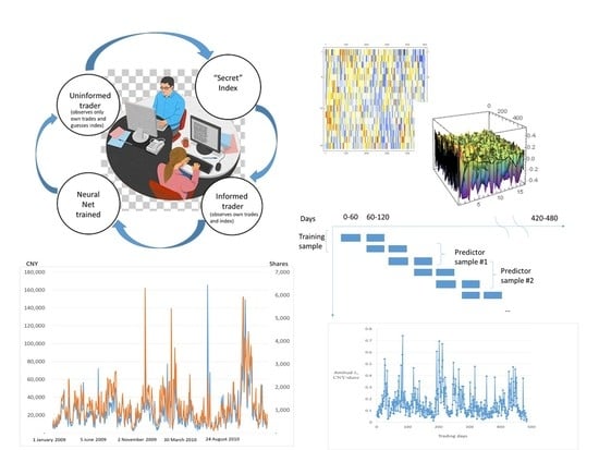
Brokerage tapes provided as Excel files have the following format shown in Figure 1.

The brokerage tapes include date, order price in CNY, type of order “buy” and “sell”, as well as the order’s volume. They did not have a timestamp in the years 2009–2010. Further on, we attribute separate spreadsheets as the “tapes” of fictitious traders from zero to four for all brokerages to conduct a natural experiment. As we can see from the data in

Table 1. Summary statistics of Brokerage 5 for all the 484 trading days during 2009–2010. (Table 1 queries the data from original datasets. Traders are marked as 0 through 4. Volume data are rounded to one share. The stock price is expressed in the Chinese Yuan. The index B or S refers to a “Buy” or a “Sell” order on a given tape. We used sample volume variance as an indicator of volume dispersion. The daily standard deviation of the volume can be approximated as √484 times √SVV. There is no systematic difference between the first four tapes, while records in the fifth tape gravitate towards higher-priced stocks.

Tape No./Type of Order	No. Trades	Min Price, CNY	Avg. Price, CNY	Max Price, CNY	Std. Price, CNY	Avg. Daily Volume	Sample Volume Variance (SVV)
05B	32,041	2.34	8.77	63	6.17	11,046	37,535
05S	28,513	2.36	8.63	61.69	5.83	9691	33,411
15B	31,550	2.3	9.91	74	5.94	10,792	33,999
15S	28,864	2.23	9.52	77.95	5.48	9963	29,251
25B	31,988	2.57	9.84	96	6.29	9509	22,946
25S	28,584	2.53	9.58	95.1	6.09	8468	18,797
35B	31,824	2.29	12.36	69.91	6.35	9144	29,004
35S	26,867	2.31	11.96	67.69	6.13	7632	26,000
45B	19,975	3.95	16.95	123.5	9.24	4939	38,321
45S	15,095	3.9	9.34	193.8	9.34	3906	65,500

, summary statistics for individual traders are comparable and we treat them as an extra level of randomization of our data. We plot the stock volumes and prices from one of the tapes in Figure 2. Visual inspection confirms an overall growth in trading throughout the two years, which is not surprising for a developing stock market, and includes a few spikes but no other obvious tendencies.

The tapes do not distinguish between individual stocks. Given the comparatively thin volume of trading in the stock markets of Mainland China during 2009–2010, we can only surmise that the trades within a given price bucket belong to one stock or a maximum of two stocks.

Our database included eight brokerages with the symbols rfokp4c, hvw5se4, zbe0rgv0, qwixupca, qguyi05q, gxbmxv0, q1ysmbyz, and 5vuyp3bu. Only the last three of these brokerage tapes contained complete data on the volume, which we further denote by the first symbol as “g”, “q”, and “5”. Most numerical examples in this paper, as well as the data, refer to Brokerage 5.

Even though it is likely that the division of trades between tapes is arbitrary, for later analysis we shall imagine them as belonging to separate “traders”. This corresponds to the intuitive idea that in modern high-frequency trading, the trader is a computer algorithm which arbitrarily parses the state-space.

Our tapes contain (see Table 1) several tens of thousands of trades over the period of two years. For comparison, a characteristic latency of a trading signal is τ ≈ 2–3 ms, which roughly corresponds to the computer messages cycling the circumference of New York City and its vicinity with the speed of light [6]. Inherent latency of trading quotes is even shorter, see [34], Table 1. Thus, if one wants to project this rate on the intensity of modern high-frequency trading, all the tapes of one brokerage would correspond to 7–8 min of wholesale trading. This illustrates the utility of observing emerging markets, where the tendencies requiring very large datasets to analyze can be observed with much less granularity.

4. Formation of the State-Space

We apply three stages of data analysis in our model. In the first stage, we allocate all daily orders to the price buckets. From these price buckets, we construct a state-space from the day-to-day correlations of order volumes, which we use as new vectors of our state-space.

$${\overrightarrow{X}}_t\left(x\right)={\left(Var({\overrightarrow{V}}_t)Var\left({\overrightarrow{V}}_{t+1}\right)\right)}^{-1/2}{\displaystyle \sum }_{i}Cov\left[V_{i,t},V_{i+x,t+1}\right]$$

(1)

In Equation (1), $\overrightarrow{V}=\{V_0, V_2, \dots V_n$} is a vector of the trading volumes in the buckets i, numbered from 0 to n. Cov[.,.] is a covariance of the vectors $\overrightarrow{V}$ for the lag = x between the buckets. Most of the covariances for large x are negligible (see below).

The intuition for this definition is that only a reasonably small number of price buckets contribute to this measure because a daily price change for any stock is expected to be small compared to its price. Indeed, only the price changes below 8 CNY were consistently observed on each trading day, although these changes could obviously be larger for some days.

Equation (1) was written with an assumption that day-to-day correlations of order volumes exhibit more stability than the volumes themselves. Heuristically, this assumption is supported by the existence of the unique T + 1 rule in the Chinese stock markets, according to which one has to hold stock one day or more before selling [9] so that intraday noise must be uncorrelated between today and tomorrow.

The predictive power of the correlations (if any) can be used by an informed broker in the following manner. If correlations between buckets ρ_ij were persistent, a broker could predict the migration by x in a given price bucket i, by the formula:

$$X_t^i\left(x\right)=\frac{{\rho }_{i,i+x}{V}_t^i}{{{\displaystyle \sum }}_{ij}{\rho }_{i,j,t-1}}$$

(2)

In real life, the brokers can use a next-day predictor ${\widehat{\rho }}_{ij,}$ to guess their next-day order. Note that in the 100%-efficient markets, or for markets in equilibrium, our state variable is exactly zero.

Covariance matrices could be more consistent from the mathematical point of view, but they are harder to interpret intuitively—particularly because they grow as squares of the volume with more active trading―and visualize. Moreover, covariance matrices, because of their nonlinear growth with average volume, obscure participation of the “high impact trades”, i.e., the trades, which influence price much in excess of their size (Xiaozhou, 2019). In Equation (1) we use three types of variables as “volumes”: a volume of buy trades, a volume of sell trades, and an imbalance volume, which we define as the difference between buy and sell volume at a given price bucket. In the case of imbalance statistics, our measure is reasonably similar to VPIN proposed by [12].

Our state-space is a discrete space of sixteen price buckets, separated by Δ = 0.5 CNY (daily changes of stock prices by more than 16Δ = 8 CNY were seldom observed in the sample). We split the entire trading book into 0.5 CNY buckets by the price change (a few hundred encompassing all the stock price range) but use only the first sixteen buckets. Using a larger number causes a spurious periodicity in our data. A smaller granularity will leave too few events in each bucket to allow confident averaging, while a larger granularity will average over most daily price changes. The division of the trading book into equal buckets allows us to avoid the problem that the trades in our database are not stamped with the name of a particular stock. The trading volume of all stocks experiencing “zero” or “significant” price change goes into the same bucket. Our construction of the phase space potentially allows a two-way analysis: panel analysis which is based on individual buckets and time-series analysis which follows the evolution of buckets through time.

The second stage of our analysis is building a dynamic model of trading. Our only assumption is that the state variables evolve by a linear dynamics, which we estimate from our data:

$$X_{i,t+1}\left(x\right)=X_{i,t}\left(x\right)+{\widehat{K}}_{ij}·X_{j,t}\left(x\right)+{\epsilon }_{j,t}\left(x\right){\delta }_{ij}$$

(3)

For our analysis, we use a dual state-space obtained by the Fourier transform of the initial state-space of a model. Philosophically, our choice of the state variable is based on the Bochner theorem in functional analysis, which states that covariance of a weakly stationary stochastic process always has a representation as a Fourier integral of a stationary measure [35]. Henceforth, a broad class of stochastic processes can be represented in the form above [36] (Chapters 14 and 15). Here, we only display our model in the form we had used in our analysis.

The Fourier transform of the Equation (4) gives a linear regression in dual state-space:

$$\Delta {\overrightarrow{X}}_{t+1,{\omega }^{\prime }}\equiv {\overrightarrow{X}}_{t+1,{\omega }^{\prime }}-{\overrightarrow{X}}_{t,{\omega }^{\prime }}={\widehat{\beta }}_{{\omega }^{\prime }\omega }{\overrightarrow{X}}_{t,\omega }+{\overrightarrow{e}}_{t+1,\omega }{\delta }_{{\omega }^{\prime }\omega }$$

(4)

In Equation (4), because of the Fourier transform, the vectors are assumed to be complex, i.e., with twice the dimensionality of the original state-space. The beta matrix has the dimension of 32 × 32 if we separate real and complex parts. Because our initial state vectors are real, there is covert symmetry in the coefficients and some rows in the beta matrix are identical zeroes. The Kronecker delta in the regression residual assumes that all spurious correlations between volumes disappear in one-two days.

Note that we make no assumptions about the random process governing the price dynamics. The only limitation of Equation (4) is the size of the beta matrix we use to approximate a continuous Fourier integral operator [37,38]. The Inverse Fourier transform of our beta operator is analogous to the Q-operator in [39] Markovian model of the Limit Order Book (LOB).

Original daily state vectors are recovered through the inverse Fourier transform below, where the hat denotes the predicted independent variable. They can have a small complex part because of the finite representation of decimals in the computer, which we ignore.

$${\overrightarrow{X}}_t\left(x\right),\widehat{{\overrightarrow{X}}_t}\left(x\right)=F_{\omega \to x}^{-1}[{\overrightarrow{X}}_{t,\omega },{\overrightarrow{\widehat{X}}}_{t,\omega }]$$

(5)

And

$${\overrightarrow{\epsilon }}_t\left(x\right)=F_{\omega \to x}^{-1}[{\overrightarrow{e}}_{t,\omega }]$$

(6)

In the third stage of our analysis, we employ neural networks to make sense of the regression residuals, i.e., whether they are reflecting real economic surprises or a result of noise trading. We do not know the prediction algorithms being used by the traders and, with time, they might become more complicated than anything we can devise. Therefore, we try an inverted strategy of deep learning. Namely, given an unpredictable part of the day-to-day volume correlations, we try to predict the realized indexes of the Chinese economy. The intuition behind this method is that if there is systematic unexpected buying or selling pressure in the market, it must reflect prevailing market sentiment.

5. First Validation of the Model

We have tested our model’s beta estimator for different traders in our database. Our results are represented by the sets of 484 × 16 matrices (the number of trading days during 2009–2010 times the number of the price buckets). The correlations between columns and rows of the matrix ${\widehat{\beta }}_{\omega {\omega }^{\prime }}$ for the imbalance volumes in Formula (3) are given in

Table 2. Correlations in the complex beta matrices of the linear regression.

(A) Correlation between columns of the beta matrix of coefficients for different traders.
	Tape 0	Tape 1	Tape 2	Tape 3	Tape 4
Tape 0	1	0.9620	0.9630	0.9635	0.9633
Tape 1		1	0.9618	0.9563	0.9606
Tape 2			1	0.9601	0.9678
Tape 3				1	0.9618
Tape 4					1
(B) Correlation between rows of the beta matrix of coefficients for different traders.
	Tape 0	Tape 1	Tape 2	Tape 3	Tape 4
Tape 0	1	0.9416	0.9424	0.9574	0.9431
Tape 1		1	0.9440	0.9421	0.9479
Tape 2			1	0.9635	0.9700
Tape 3				1	0.9452
Tape 4					1

. (In the series of our tests, we used Buy, Sell, Total Volume, and Imbalance indicators. The results were broadly similar across all selected measures (for instance, see Appendix B). For most of this paper, except Section 7 where we used “Buy” quotes, we selected imbalances to represent our data. In particular, imbalances can be directly compared with the “Cost of Trading” measure [40]. Complex beta matrices have dimensions 32 × 32 because of the real and imaginary parts of Fourier-transformed state vectors. Yet, under inverse Fourier transform, because of the internal symmetry, both the prediction and residual vectors are real.

We display temperature maps of an estimation of a single tape in Figure 3.

Correlations of beta matrices, Equation (4), computed between columns and rows for the temporal correlation of imbalance volumes (see Equation (1)). Tape numbering corresponds to the rows in Table 1. Correlations are symmetric across the diagonal. All the correlations between coefficients are insignificantly different from unity.

In testing regression (3) for the five data tapes, beta matrices are practically identical despite the state vectors being vastly different. This suggests the robustness of our model for the predictable component of the daily correlation of the imbalances. A similar picture was also observed from correlating betas between Buy and Sell tapes.

6. Predictable Component of the Bid-Ask Volume Correlations

As a criterion for the quality of approximation of the Equations (5) and (6), we use the vector error estimator for the predictor and the residuals:

$$\begin{array}{c}{F}_n=\raisebox{1ex}{$1$}\!\left/ \!\raisebox{-1ex}{$T$}\right.{\displaystyle {\displaystyle \sum }_{t=0}^T}{{\overrightarrow{\epsilon }}_t}^2\left(x_n\right)\\ P_n=\raisebox{1ex}{$1$}\!\left/ \!\raisebox{-1ex}{$T$}\right.{\displaystyle {\displaystyle \sum }_{t=0}^T}{{\overrightarrow{\widehat{X}}}_t}^2\left(x_n\right)\equiv {\sigma }^2\ast \left(1-\raisebox{1ex}{$F_n$}\!\left/ \!\raisebox{-1ex}{${\sigma }^2$}\right.\right)\\ {\sigma }^2=\left(\raisebox{1ex}{$1$}\!\left/ \!\raisebox{-1ex}{$T$}\right.{\displaystyle {\displaystyle \sum }_{t=0}^T}{{\overrightarrow{X}}_t}^2\left(x_n\right)\right)\end{array}$$

(7)

where σ is the empirical volatility of the data and $\widehat{X}$ is the estimate from the regression of Equation (5).

In Equation (8), we retained the multiplier and 1/T, T = 484 (trading days) in the denominator as well as the numerator for clarity. Index n = 1 ÷ 16 numbers a vector of the state-space. A typical plot of variances of the predictor and the residual is given in Figure 4.

We note that the predictor and the residual time series by construction have zero correlation. However, the coincidence of time-weighted variances between the price buckets in Figure 4 is quite impressive and it is typical for a tally of the imbalances.

For quantifying the determination of regression prediction and regression residuals, we used running correlations of panel variances for the 484 trading days in the sample. The matrix of these correlations is provided in

Table 3. Mutual determination of variances (||ρ_ij||=||r_ij²||) for the regression predictions and the regression residuals.

Traders’# Prediction/Residuals	1	2	3	4	5
1	0.4126	0.0050	0.0003	0.0002	0.0006
2	0.0001	0.3081	0.0410	0.0052	0.0052
3	0.0003	0.0219	0.3639	0.0390	0.0374
4	0.0007	0.0039	0.0163	0.3408	0.0364
5	0.0001	0.0010	0.0219	0.0140	0.4027

. From this matrix, we observe that 30–40% of the daily variability of the traders’ samples and 50% of the monthly variability is contributed by the prediction variance, and the rest by the regression residuals. The same observation that the variance of the empirical distributions is being split approximately 50:50 between the predictor and the residual can be made from Figure 4.

Table entries are the squares of $r_{ij}=Correlatio{n}_t[Va{r}_{\Delta }({\widehat{Y}}_i), Va{r}_{\Delta }({\epsilon }_j)]$ where i = 1 ÷ 5 and j = 1 ÷ 5 are individual traders indicating the explanatory power of linear regression.

Correlations between different brokerage tapes are statistically insignificant. This exercise suggests that the trader’s samples are independent in the sense of linear regression. For the trader, it means that processing data from another trader by linear regression does not contribute any valuable information. Individual traders can fairly predict their correlations between today’s and the next day’s volumes, i.e., persistence of their own demand across all price buckets, but not correlations for other traders.

7. Analysis of the Phase Space Regression Residuals

The model of Equations (3) and (4) describes a predictable component in the day-to-day correlations of trading volume of price migrations including the zeroth price bucket (price changes below 0.5 CNY). Residuals contain both microstructure noise and reactions to unpredictable economic events in the market. To analyze the residuals, we employ several methods inspired by neural networks.

We do not know what kind of training algorithms traders might be using, given the quick progress in the algorithmic finance and computation power since 2009–2010 and even as this paper is being written. Henceforth, we employ the following method. Instead of a prediction of the out-of-sample trading data, we attempt backdating market data through a simulated experiment, namely, a neural network trained by our order data attempts to predict the Chinese market sentiment index, returns on the Shanghai stock index, and yields on the bellwether 10-year bond of the Bank of China (for details of the protocol, see below). Because of the monthly periodicity of the sentiment index, for the consistency of our tests, we used monthly stock returns and monthly bond yield as well.

In our case, real-life trading algorithms would have to predict the “unexpected” direction of price changes imprinted in brokerage orders given their information on the markets. Yet, we assign to our imagined traders—represented by the brokerage tapes—a much simpler task of predicting a monthly index given their observation of the day-on-day correlation of orders within a given range of price change. (This reasoning is based on an unproven but intuitive assumption that an economically simpler problem—guessing a “covert” index from proprietary trading data rather than the other way around— is less demanding algorithmically).

Our procedure corresponds to the following stylized situation. We select a randomly chosen “informed” trader who observes orders from her own clients and trains her network by predicting the index. We use her data as a network input and then simulate the behavior of other traders whom we consider uninformed as to the direction of the three chosen indexes but who controllably can observe or be in the dark concerning the actions of their colleagues from the same brokerage (Figure 5).

The situation of “leaky brokers” has been described in [41] in the following terms: “When considering the theoretical soundness of a market equilibrium in which brokers leak order flow information, one may wonder why an informed asset manager is willing to trade with brokers that tend to leak to other market participants… The broker would enforce this cooperative equilibrium across subsequent rounds of trading. In particular, the broker can exclude from the club the managers that never share their private information and reward with more tips the managers that are more willing to share”.

The results were averaged over six or twelve independent runs of the network and were not significantly different.

The best results were obtained by a seven-layer convolutional neural network (CNN), though other options have been explored (Appendix C). Conventionally, CNN is used for image recognition and analysis. Essentially, we used matrices of the residuals of the output regression (depicted as a heat map of the matrix in Figure 3) as if they were digitized information for the visual images to predict the direction of an index.

Table 4. Correlation of predictions of the three indexes. Traders “a” and “b” were designated as informed about the index. The first two columns include informed traders in both training and prediction samples. The second pair of columns include data from an informed trader only in the training sample. The third pair of columns does not have an informed trader at all. For comparisons, we show the results obtained by a single 500 round and by changing ReLU into the TANH perceptron function. The lower left rectangle indicates data obtained from six TANH trials.

(A) Correlations of monthly predictions based on market sentiment with actual data.
Predicted Index	Sentiment
Traders Training-Predict	a–c	b–c	b–c	c–d	c–d	d–e
	0.9756	0.9382	0.9505	0.9531	0.912	0.9166
	0.9527	0.9643	0.9474	0.9669	0.9346	0.9014
	0.9545	0.9007	0.9232	0.9399	0.9455	0.9307
	0.9684	0.9518	0.9483	0.9695	0.9569	0.966
	0.9727	0.9364	0.9676	0.9699	0.9344	0.9431
	0.9697	0.9371	0.9476	0.9636	0.9581	0.9225
Average	0.9656	0.9381	0.9475	0.9605	0.9403	0.93
t-statistic 10%	0.0139	0.0307	0.02038	0.017	0.0249	0.0324
(B) Prediction of the returns on the Shanghai stock market.
Predicted Index	Stock Index Return
	a–c	b–c	b–c	c–d	c–d	d–e
	0.4169	0.4056	0.6882	0.7065	0.182	0.2083
	0.5363	0.3775	0.437	0.4296	0.5341	0.182
	0.1017	−0.1194	0.2451	0.2789	0.451	0.1656
	0.0537	0.3293	0.2767	0.4279	0.2528	0.0906
	0.3947	0.4636	0.677	0.4051	0.0693	0.4107
	0.431	0.3038	0.3851	0.3717	0.3207	0.6272
Average-6	0.3223	0.2933	0.4515	0.4366	0.3017	0.2807
t-statistic at 10%	0.2826	0.3023	0.2766	0.2067	0.2472	0.2889
Average-12	0.3385	0.271
t-statistic at 10%	0.228	0.2374
(C) Predictions of the yield of the bellwether Chinese bond.
Predicted Index	The Yield on a 10-Year BOC Bond
	a–c	b–c	b–c	c–d	c–d	d–e
	0.002	−0.1425	−0.0575	−0.0281	−0.1188	−0.0296
	0.0413	−0.1958	−0.0556	0.1921	0.1953	0.0502
	−0.0729	−0.1434	−0.2029	−0.1040	0.1149	−0.1185
	0.0019	0.0006	0.3416	0.062	−0.0514	0.1155
	0.1427	0.2798	−0.0575	−0.170	−0.3020	−0.4854
	−0.5078	−0.3818	0.1061	0.0081	−0.1738	−0.0613
Average	0.1766	0.1078	0.0546	0.1236	0.1079	0.1032
t-statistic at 10%	0.1819	0.299	0.2623	0.1793	0.27	0.226
500 Rounds	0.1415	0.2063	−0.2305	0.1633	−0.1407	−0.2493
TANH	−0.0517	0.3209	−0.2302	0.0754	0.02279	−0.0748
t-statistic at 10%, TANH					0.2755	0.3273

displays the trials with randomly selected informed traders in both training and predictive samples, as well as training samples with only “uninformed” traders, i.e., the traders who observe only bid and ask volumes per basket, without access to current or past magnitudes of the index. Unlike the results from

Table A1. Select runs of a 10-layer neural network for the backward prediction of monthly indexes from traders’ activity. Capital letters B, S, and I mean “Buy”, “Sell”, and “Imbalance” samples of residuals. Letters from a-d refer to a particular trader. An arrow designates training vs. prediction tapes. The symbols r_1–3 refer to the correlation coefficients of the neural network predictor and the actual indexes. The explanatory power of the predictions can be inferred from the squares of the correlation coefficient. For instance, if we treat broker “b” as informed, trader “a” could have predicted bond yield for the next month from their imbalances with an explanatory power $\rho =r_3^2={0.5178}^2\approx 26.8\%.$ Test results were poorly reproducible on successive runs of the network.

Trader/B, S, I	Sentiment, r1	Market Return, r2	BOC Bond, r3	Notes
Bb → Ia	0.0389	0.4099 (−0.2888)	0.5178	(Tanh) instead of ReLU
Bb → Ib	−0.1663	0.2607	−0.1339
Bb → Ic	0.3075	−0.3951	−0.2713
Bb → Id	0.4600	0.3936	0.2525
Sb → Bc	−0.0431	−0.3944	−0.2389	Control
Ic → Bb	−0.2255	−0.3282	0.1444	Control

in Appendix C, the statistically significant results from Table 4 were broadly reproducible on successive runs of the network.

The general conclusion from Table 4 is that CNN can reliably predict Chinese market sentiment from daily imbalances, prediction of the stock market returns is usually significant at 10% but not at 5%, and the yield of BOC bond cannot be inferred from the imbalances.

The implication of insider information does not improve prediction very much for the market sentiment index, somewhat helps to predict the direction of the stock index but well within the assumed 10% statistical dispersion of the results, and is irrelevant for the direction of bond yields. In all cases, there is little difference whether an “uninformed” trader trains her network on the imbalances of her informed colleague or another uninformed trader.

8. Discussion: Possible Sampling Issues

Reporting files do not contain identification of the execution price and a particular stock. Our formation of the price buckets was based on a uniform division of the price range in a trading book into the intervals of 0.5 CNY. We considered this choice optimal because it allows a significant number of price buckets (120 ÷ 400). Furthermore, migration of the price for more than 8 CNY in a given day is rare, and we can use a parsimonious 16×16 matrix approximation for the Fourier evolution operator.

This, or any similar choice―for instance, an arbitrary 0.4317 CNY―assures that there could be one, several, or no trades in a particular price bucket. Yet, the Chinese stock market, which, in 2009–2010 was in its nascence, was dominated by the low-priced stocks (below 10 CNY). At the end of 2009, of the 293 listed equities, only 34 issues (11.6%) had a mean price below 10 CNY, and 259 had a price above that number. Henceforth, the lower price buckets could be systematically different from the upper buckets in that they might contain several stocks, while the price buckets above the average (see Table 1) can contain only one stock or none altogether.

To clarify this problem, we artificially split the trader books into parts comprising the stocks with the price below 10 CNY and above 10 CNY. Of course, there could be some borderline migration of stocks priced slightly above 10 CNY into the first portfolio and stocks priced slightly below into the second. We expect a small influence of this issue on day-to-day trading and we ignored it in our analysis. When we accomplished the procedure described in Section 4, Section 5, Section 6 and Section 7, for our censored trading books, the results were broadly the same as having been observed in Table 4. Namely, if one uses portfolios of low-priced stocks to train the net and then predict the index from the trading books, in which only the high-priced stocks are included, one can confidently infer the sentiment index; the Shanghai stock index is predicted in some runs but with low statistical validity, and there are no correlations between the net trained our traders’ positions and the yields on the 10-year bond of the bank of China. These results do not change much if we train the net on the high-priced stock and leave the prediction to the trader of the low-priced stock. Only the prediction of the sentiment index slightly improves (correlation grows from ~95–97% to ~97–99%), which suggests that the higher-priced stock was more liquid and, henceforth, had a better predictive value. As is the case with all statistical experiments, this observation is only tentative.

9. Empirical Liquidity of the Chinese Stock Market in the Period 2009–2010

A proposed microstructure model of the Chinese stock market allows us to analyze both predictable and unpredictable frictions resulting from two interleaving factors: (1) imperfect balance between buy and sell orders, and (2) securities changing value during trading.

The net cost of trading is computed similarly to [40], though their formula can accept different conventions. Our formula presumes that the brokerage sells an asset in today’s quantity marked to market at yesterday’s buy price and replenishes its inventory sold yesterday at today’s ask price, with the cost to the customer being the same in value and opposite in magnitude. Of course, the signs in Equation (9) are arbitrary.

$${\pi }_{ti}=p_{ai,t-1}{V}_{b,t}-p_{bi,t-1}{V}_{s,t}$$

(8)

In Equation (9), π_t is our definition of the cost of trading, and p_a, p_b are the ask/bid price buckets. The V_b, V_s are the volumes of buy/sell orders. The index i = 1–16 signifies the price bucket. Note that in market equilibrium, in Equation (7), cost averaged over all buckets is equal to the (constant) bid-ask spread times the daily turnover and is always non-negative. Outside of equilibrium, the sign of ${\pi }_t$ can be arbitrary because of fluctuating stock prices.

Our analysis by CNN indicates that the net cost of trading is a fair predictor of the market direction in the sense that we have outlined in a previous section (Figure 5). Namely, if we assume that the broker or regulator is “blind” to the order size, she can get a clear idea about the Chinese market sentiment from the trading costs only. Their idea of stock market direction would be imperfect but statistically significant and, finally, there is no connection to the Bank of China bond prices through our model.

While this exercise is purely imaginary as being applied to the Chinese brokerages, we suggest that this conclusion—that, in the observed period, trading costs reflected market sentiment more or less mechanically (see Figure 6)―can help traders and regulators alike in the case of “Dark Pools”. In the latter case, the information about the exchange’s strategy is covert and can be gleaned only indirectly.

The Equation (9) can be recast in the (dynamic) version of [20] liquidity measure. Namely,

$${\lambda }_{ti}=\frac{\left|{\pi }_{ti}\right|}{\raisebox{1ex}{$\left(V_{b,t}+V_{a,t-1}\right)$}\!\left/ \!\raisebox{-1ex}{$2$}\right.}$$

(9)

Further on, we use liquidity lambda to predict the same indexes. The intuitive meaning of our version of the Amihud measure is that it represents the average cost for the agent to make a roundtrip inside the same price bucket with one share. To provide a glimpse of the magnitude and volatility of λ, we display its daily dynamics in Figure 7.

10. Single Event Analysis

Our sample includes a day of the Flash Crash in US stock markets (6 May 2010), which means, dependent on daytime, either trading day 326 or 327 in our sample. There is no visible anomaly in the liquidity of the Chinese stock market during or after that day. It is interesting to analyze this event using our methods.

The spillovers from the established stock markets into the Chinese markets had previousy been studied by [42] using the measure of volatility proposed by [43,44]. They observed that before 2010, the Chinese stock market produced volatility spillovers to Taiwan and Hong Kong, but its influence on the European and North American markets was statistically insignificant. However, the shocks in the US stock market affected every stock market they studied. Beginning in approximately 2007, some pushback from the Chinese stock market could be observed.

The question of whether the mutual influences between the stock markets were macroeconomic or microstructural in nature was investigated by [22]. They also observed asymmetric shocks, i.e., the shocks propagating predominantly from US markets into China but not the other way around. Li and Peng noticed that a structural shock in the US markets usually decreases correlations between the Chinese and American stock markets.

We decided to investigate the influence of the US stock markets on China by our methods of the CNN analysis of the regression residuals. We display the testing strategy in Figure 8. The observation period (years 2009–2010) is split into eight overlapping samples of 60 days each. One sample of two adjacent periods (usually, but not necessarily the first) is used for network training. This constitutes one training and five predictor samples. We then attempt to predict monthly indexes backward from the training data. The null hypothesis is formulated as follows:

Hypothesis 1 (H1).

For i = 1 ÷ 5, Correlation [Index prediction from λ_i, Index] = Correlation [Average[λ], Index].

Hypothesis 2 (H2).

For at least one i, Correlation [Index prediction from λi, Index] ≠ Correlation [Average[λ], Index].

The intuitive meaning of the null hypothesis above is that predictions obtained from subsamples of illiquidity measures are no different from each other. We, of course, would prefer that the null be rejected for the samples containing the Flash Crash in America.

The statistical significance of the correlations of the predicted monthly indexes for one of the traders (tapes) is shown in

Table 5. Probabilities of null hypothesis H1 from a typical correlation test of index predictions from Amihud λ.

(A)
Trading Days in the Sample	P from Pearson	P from Spearman
120–240	0.364	0.932
180–300	0.605	0.976
240–360	0.227	0.062
300–420	0.847	0.342
360–480	0.975	0.903
(B)
Trading Days in the Sample	P from Pearson	P from Spearman
120–240	0.4	0.712
180–300	NA	0.561
240–360	0.452	0.437
300–420	0.857	0.806
360–480	0.616	0.061
(C)
Trading Days in the Sample	P from Pearson	P from Spearman
120–240	0.622	0.285
180–300	0.721	0.565
240–360	0.926	0.743
300–420	0.688	0.554
360–480	0.167	0.143

. Note that, in agreement with the results of Section 6, almost no statistically significant correlation of prediction of the return on the stock index and none for the yields on the 10-year bond can be observed. On the contrary, the prediction of the market sentiment from an observed Amihud illiquidity measure is robust. This corresponds to the testing of H1, and of H2 above where the right-hand side is replaced by zero.

As a rule, null cannot be rejected for any of the three indexes. (A) Probabilities for prediction of sentiment index, (B) probabilities for prediction of stock market returns, and (C) probabilities for prediction of bond yields. Highlighted are the subsamples, which include the US Flash Crash of 6 May 2010.

We observe from Table 5 that the null hypothesis―illiquidity in the subsamples that include the date of the American Flash Crash behaves any different from other samples—cannot be rejected. Only one probability in Table 5 is below 10%, and it is not stable with respect to the consecutive runs of the neural network with a different seed.

We cannot discern an influence of a shock from microstructure data, yet the results, e.g., of Li and Peng (2017), suggest that the transmission of shocks was real. This suggests that the transmission between the US and Chinese markets was mainly through macroeconomic fundamentals. As we have seen from Table 5, our deep learning-based method could simply require too long a sample to resolve the spillover.

11. Conclusions

In our paper, we propose a microstructure model of the Chinese stock market. We build it from a state-space of interday correlations of volumes between price buckets. Because of the T + 1 rule in the Chinese stock markets, interday correlations are expected to significantly reduce the microstructure noise. For the 100%-efficient market in equilibrium, our time series would be exactly equal to zero.

This model is analyzed by OLS in a dual state-space, connected to an original state-space by a Fourier transform across the multiple price buckets. This procedure corresponds to an approximation of the predictable fraction of the time evolution of trading volumes by a Fourier integral (pseudodifferential) operator of a general form. In a discrete case, this operator can be represented by a matrix of arbitrary dimension (selected by convenience as 32 × 32) acting on the space of the Fourier coefficients (see Appendix A for details). This method is completely general and can be applied to any time series, which can be grouped into panels, in our case volumes per a given stock price.

The presented model based on the Fourier integral operators, augmented by the deep learning methods, can be calibrated daily by the market makers. It predicts the next day’s volume at a price change x (see Equation (2)) and has no fundamental price inputs. Henceforth, the prediction reveals the dynamics of brokerage demand driven by its clientele without intervening events in the market.

The proposed method (or protocol, in the parlance of the deep learners: (1) preprocessing, filtering using Fourier Integral Operators; (2) processing, recognition of the sequence of residual matrices using neural network; (3) postprocessing, index forecast with a trained network) is universal and can be applied to any trading system as a continually updated model. It can simulate any given market with a level of complexity chosen by the broker and/or the regulator. Namely, each day, a predictable trading forecast is provided by a multivariate filter (Fourier Integral Operator in the current paper, but other methods, e.g., Kalman filter, can be used as well). This stage is “dumb”, in the sense that it does not take into account intervening changes in market fundamentals. Past residuals to the regression can be independently predicted by the neural network and added up to the results of the filtering. In the third stage, different validation strategies can be applied. This protocol can incorporate generic processes such as multivariate ARMA (similar to the one used in the paper) or a specific microstructure model, e.g., Roll’s [4].

The main conclusion of our analysis is that the unpredictable dynamics of trades completed by the Chinese brokers in the period 2009–2010 were tightly correlated with the Chinese market sentiment in a highly nonlinear sense of machine learning. This can be interpreted as investors trading according to the available market information they receive. The returns on the stock index were predictable, but statistically they were barely significant. Because the predictive power of the trades for the actual stock market returns was small, this indicates investors were following a herd mentality. We observed no connection between the trading activity and the yields on the bellwether 10-year bond of the Bank of China. This may signify that the market risk in an emerging market, which describes the Chinese stock market in 2009–2010, has only a small dependence on prevailing borrowing rates.

Finally, we tested whether the Flash Crash of American markets on 6 May 2010, was reflected in the liquidity of the Chinese stock market. For this, we used a dynamic version of the Amihud illiquidity measure λ. The illiquidity measure predicted by the CNN was almost as good a predictor of market sentiment as the VAP (see Figure 6), and we used it to analyze a possible contagion of the American Flash Crash on the Chinese markets.

With our methods, we did not find any statistically significant evidence that liquidity was higher or lower than the average during the period preceding or following the Flash Crash. This indicates a need for a finer measure of contagion between American and Chinese stock markets. In particular, samples of 60 days long can be too crude to resolve the influence of the Flash Crash, which may have lasted only 1–2 trading days.

The limitations of the proposed method are that all regressions at the preprocessing stage must be linear. Non-linear regressions lead to the non-linear integral operators on the right-hand side, which may be more complicated or less computationally stable than the original equations.

The second limitation is that the choice of neural network (discussed in Appendix C) can be rather arbitrary with few hard-wired criteria to guide the selection. Moreover, the main limitation of this study is its restricted array of free data from the Shenzhen Stock Exchange and its limited computer resources. (All computer algorithms were tailored to be run on a conventional PC using not more than 15–30 min of processor time in the case of R algorithms.) However, all of the paper’s methods can be applied to datasets of arbitrary size.