Abstract
Several papers on distributions to model rates and proportions have been recently published; their fitting in numerous instances is better than the alternative beta distribution, which has been the distribution to follow when it is necessary to quantify the average of a response variable based on a set of covariates. Despite the great usefulness of this distribution to fit the responses on the unit interval, its relevance loses objectivity when the interest is quantifying the influence of these covariates on the quantiles of the variable response in ; being the most critical situation when the distribution presents high asymmetry and/or kurtosis. The main objective of this work is to introduce a distribution for modeling rates and proportions. The introduced distribution is obtained from the alpha-power extension of the skew–normal distribution, which is known in the literature as the power–skew–normal distribution.
Keywords:
unit distribution; linear regression; maximum likelihood estimation; score function; information matrix MSC:
60E05; 62J05
1. Introduction
Random variables for rates and proportions (bounded data) are very common in different areas of knowledge such as medicine and economics. There are also some statistical distributions for fitting this type of variables, given their asymmetry and/or kurtosis. However, in different scenarios, these variables have been accompanied by a set of explanatory variables having more complete explanation of the phenomenon. Among the asymmetric probability distributions that stand out are Azzalini’s skew–normal [1] and generalized Gaussian power–normal, see Durrans [2] and Pewsey et al. [3], which have been extended over the last few decades to other types of distributions. These families of distributions have their support in the whole set of the real numbers, implying in a double-truncated distribution for data in the unit interval , whose procedures of estimation of the parameters are quite complex. Martínez-Flórez et al. [4] studied a distribution for rates and proportions by using the power–normal distribution. Probability distributions for bounded random variables are common in the statistical literature, with those that stick out being beta distribution in classical statistics and some bounded extensions as in the case of unit–Birnbaum–Saunders, unit–Weibull and unit–Lindley distributions by Mazucheli et al. [5,6,7].
Along this same line of unit distributions and their extensions to the case of regression models, more recent works are also highlighted, such as: the unit-generalized log Burn XII, unit-folded normal, and unit log–log distributions, see [8,9,10]. Furthermore, for the specific case with covariables, there are well-referenced works, among them, the beta-regression model of Ferrari and Cribari-Neto [11] and Ospina and Ferrari [12], whereas Martínez-Flórez et al. [13] studied a double-censored model for random variables on the unit interval. More recently, we find the works of Korkmaz et al. [14], Mazucheli et al. [15,16].
The skew–normal (SN) distribution, with asymmetry parameter , denoted by , was studied by Azzalini [1] and its probability density function (PDF) is represented by , for , where and and represent the PDF and the cumulative distribution function (CDF) of the standard normal distribution, respectively. Here, the parameter controls the asymmetry in the distribution. The CDF of a random variable following an distribution is given by,
where is the Owen’s [17] function given by
The power–normal (PN) distribution, denoted by , with PDF given by,
where and is a shape parameter, was introduced by Durrans [2]. The PN distribution has been multiple applications in cases where the distribution of data presents high or low asymmetry and/or kurtosis when compared to normal distribution. A more flexible extension of the SN and PN distributions was studied by Martínez-Flórez et al. [13]. This extension is called power–skew–normal and has PDF given by
for , where and . These authors found out that the asymmetry coefficient for the PSN distribution is the interval, while the kurtosis is in the interval. Furthermore, according to the results by Azzalini [1] and Pewsey et al. [3], the PSN distribution contains the asymmetry and kurtosis ranges of the SN and PN distributions, being able to fit data with higher (or less) skewness and kurtosis than allowed by these two distributions. In this work, we extend this distribution to the case of bounded random variables on the range, and study its main properties and the process of estimating its parameters.
The rest of the paper is organized as follows. In Section 2, the unit-power-skew-normal distribution is introduced and its main properties are studied. The inference process by using maximum likelihood method is carry out. In Section 3, explanatories variable in the unit-power–skew–normal distribution are introduced and, the statistical inference is performed. The resulting model is called the unit–power–skew–normal regression model. In addition, the score functions and the elements of the observed information matrix are obtained. The Section 4 presents the results of two simulation studies. Two applications with real data to illustrate the applicability of the proposed methodologies are presented in Section 5. Finally, in Section 6, the extension of the unit–power–skew–normal distribution to the bivariate case is explored.
2. The Unit–Power–Skew–Normal Distribution
Performing the transformation , where , is obtained the extension of the PSN distribution for the case of positive random variables, which is called log–power–skew–normal distribution (LPSN). The PDF of the LPSN distribution with parameters and , denoted by , is given by:
In addition, the PDF of the location-scale family of the random variable with LPSN distribution is
where , with the location parameter, and the scale parameter. Now, by applying the transformation on the LPSN distribution, it is obtained the distribution with PDF given by
where , , and . The distribution in Equation (4) is called unit–power–skew–normal and is denoted by . The UPSN distribution has some interesting features, for example, if and the unit–normal (UN) distribution is achieved, and is denoted by . For , the unit–power–normal (UPN) distribution, is obtained and, for , the unit–skew–normal (USN) distribution is obtained. In this way, the UPSN distribution encompasses three families of distributions that can be used in the fit of data in the unit interval .
2.1. Properties
The CDF and survival function of the distribution are, respectively, given by:
and therefore, the hazard function is defined by:
while the inverse hazard function is given by
As a result, the cumulative hazard function can be obtained from the survival function through the relationship:
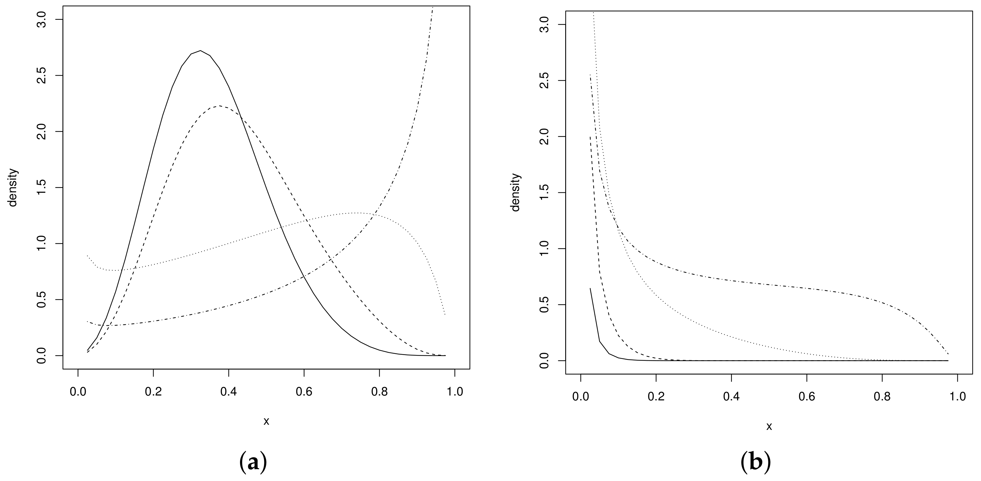
Figure 1a,b shows the UPSN density behavior for some parameter values. It can be seen in Figure 1a that the UPSN distribution presents different asymmetric shapes to the right and to the left. Furthermore, decreasing forms of the distribution are observed in the support of the variable, and decreasing forms (See Figure 1b). These different behaviors of the pdf allow it to fit data with a wide variety of shapes and behaviors, especially with high kurtosis degrees, considering that this is one of the benefits of the power–normal distribution family (see [3]).

Figure 1.
UPSN distribution for and (a) values of (dotted–dashed line), (dotted line), (dashed line) and (solid line), (b) values of (dotted–dashed line), (dotted line), (dashed line) and (solid line).
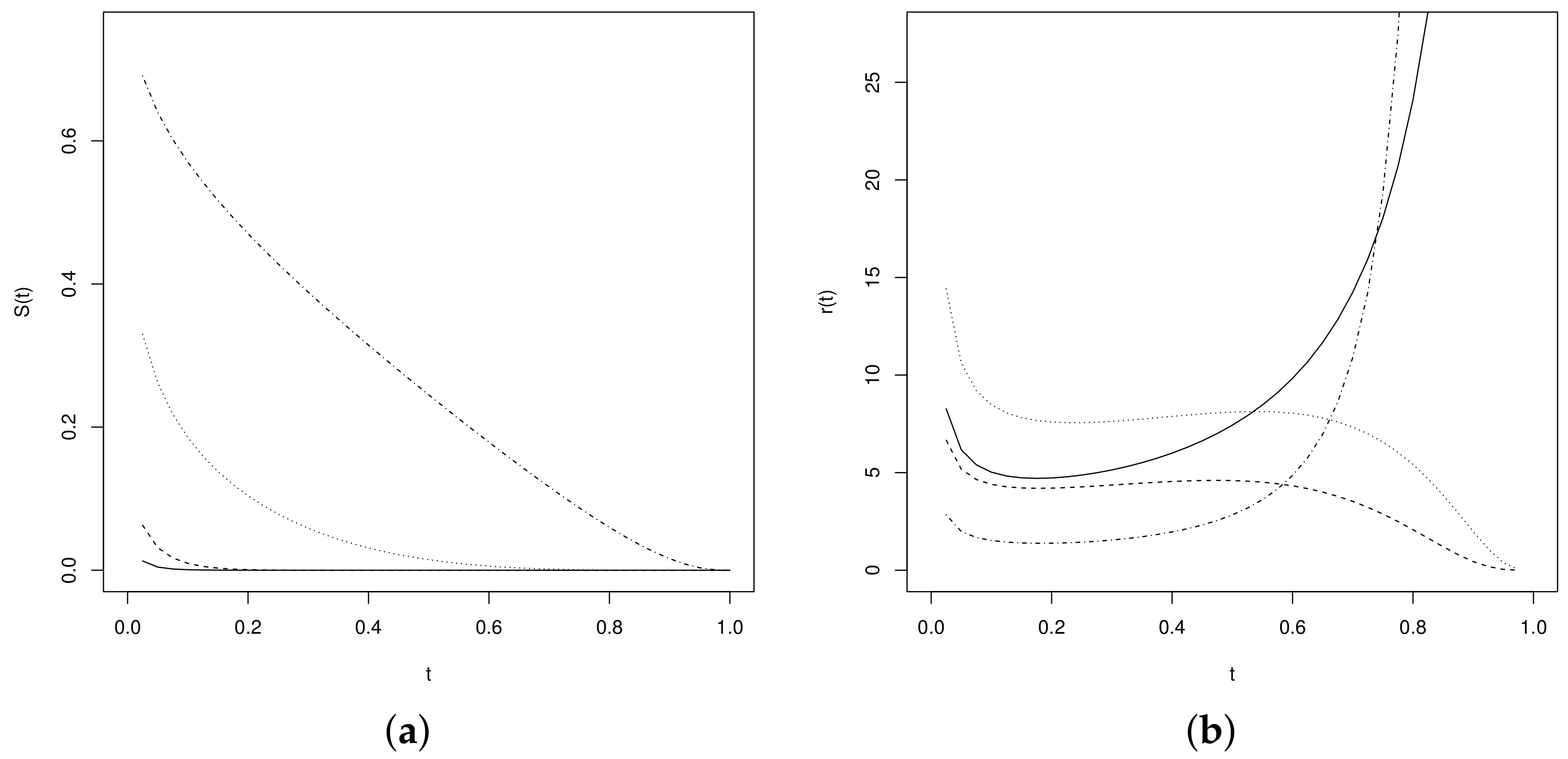
Likewise, the graphs of the Figure 2 exhibit the behavior of the survival and hazard functions.
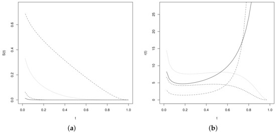
Figure 2.
Survival and hazard functions for , and values of (dotted–dashed line), (dotted line), (dashed line) and (solid line) (a) and (b) .
To generate a random variable with distribution can be done using (5) using the inversion method. Thus, for a uniform random variable U, on , we have that the random variable
follows a , where represents the inverse function of . From this result, it follows that also follows a distribution.
2.2. Moments
Moments of the standard distribution can be obtained from the relationship , where . Thus, for , we have
where represents the moment-generating function (MGF) of the random variable . Now, by performing and using the transformation method, it can be demonstrated that
then,
and, since is a non-decreasing function such that, , and given that , it follows , that is,
whence it follows that
that is, moments of the UPSN distribution exist can be obtained from the relationship
Using the usual definition, the r-th moment of the standard UPSN distribution is given by
The centred moments in mean, , for can be calculated by the expressions:
Furthermore, the variance and coefficient of variation, skewness and kurtosis coefficients are given by:
From expression (7), it is possible to calculate the moments of the UPSN distribution. The Table 1 shows the values of , , and the skewness and kurtosis coefficients for a random variable with UPSN distribution in its standard form, that is, for some selected values of the parameters and . In addition, for values and some values of between and 25, we find that the ranges of skewness and kurtosis coefficients are and , respectively.

Table 1.
Moments for a random variable with UPSN distribution.
2.3. Statistical Inference
For the estimation of the parameters of the distribution, we use the maximum likelihood (ML) method. Thus, given a random sample , with , for the log-likelihood function of the parameter vector , except for the constant, is given by:
where .
The elements of the score function , and defined as the derivative of the log-likelihood function with respect to the parameters, that is, , for , where , , and , they can be expressed by:
where , and /, for .
By setting each of these functions equal to zero, the score equations are obtained and their respective solutions are obtained by using iterative numerical methods, leading to estimates of the distribution parameters. From the score equation , we have
we arrive to the profiled log-likelihood, except for the constant,
whose maximization leads to the ML estimates of the parameters and , where
The observed () and expected () information matrices can be obtained, respectively, by finding and , where is the Hessian of It can be shown that for the information matrix of this distribution is non-singular (the matrix for the case was studied in Salinas et al. [18]). Thus, for large sample sizes and under regular estimation conditions, that is, continuity and existence of the pdf and its first three derivatives, consistency of the estimator and existence of the information matrix, we have that the vector converges to a normal .
Let us remember that, the exponentiated-normal family of distribution is regular, see [19]. In addition, Martínez-Flórez et al. [20] showed that the family of EFAN distributions satisfies all the regularity conditions; therefore, the exponentiated-normal family also satisfy them, since this is a particular case of the EFAN model by taking .
3. The USPN Regression Model
In many situations, the response variable X is explained by a set of exogenous variables through the intrinsically linear relationship
where , being the response for the jth variable measured on the ith individual, for and ; is a vector of unknown parameters that must be estimated, and . It follows that, for , .
From this perspective, this model could be seen as a generalized linear model with link function and random component . Even here, this model could be extended to the non-linear case in the parameters by making a doubly differentiate continuous function. Similar to the case without covariates, for cases and a unit–normal–regression model is obtained, whereas for a unit–power–normal regression model is obtained. The unit–skew–normal regression model is followed when .
The log-likelihood function of the parameter vector of the model is given by:
where . The score function corresponding to the log-likelihood function is given by (for )
Similar to the case without covariates, by matching the score functions to zero, we obtain the system of score equations, whose solution, using iterative numerical methods, leads to the maximum likelihood estimates of the model parameters.
After intensive calculations, the elements of the observed information matrix, , for the parameter vector were obtained. These elements are defined as minus the second derivative of the log-likelihood function with respect to the parameters, this is,
The elements of the matrix are presented explicitly in the Appendix A.
For large n, the observed information matrix converges to the expected information matrix. Thus, from the elements of the matrix, the errors of the model parameters can be estimated, for , calculating the square root of the diagonal elements of . By denoting by the kth element of the matrix, confidence intervals can be obtained for model parameters, especially for , . For a confidence level of 95%, the confidence intervals for the parameters are given by: for
4. Simulation Study
To study the behavior of the maximum likelihood estimators (MLE) of the parameters of the UPSN distribution and the UPSN regression model, we conducted two Monte Carlo simulation studies. In the first simulation, we considered the distribution with values for the parameters: ; ; ; and , and . The considered sample sizes were and 1000, and the number of samples for each scenario was 5000.
To evaluate the performance of the estimators, the absolute value of the bias (AVB) and the root–mean–square error (RMSE ) were considered, which are given by:
respectely, where is the estimator od for the jth sample, for . In the two simulations, the maxLik function [21] of the statistical software R Development Core Team [22] was used and the optimization of the likelihood function was performed by using iterative methods based on the Newton–Rapshon algorithm.
The obtained results for each estimator for the UPSN distribution can be seen in Table 2. In can be observed that, as the sample size increase, the bias (in absolute value) and the square root of the mean square error decrease, indicating a good behavior of the MLE of the parameters of the UPSN distribution. This guarantees the asymptotic consistency of the MLE of the parameters of the distribution in question.
Table 2.
MLE behaviors for the UPSN Distribution.
In the second simulation study, we considered the UPSN regression model defined in Section 3. We considered the following simulation scenarios: and for , and ; and and for , and . The covariate vector was , with v being generated from a uniform distribution . For each simulation scenario and the sample sizes and 1000, 5000, we generated random samples of the UPSN regression model , . To evaluate the performance of the estimators, the AVB and RMSE were again used. The results of the estimates are found in Table 3.
Table 3.
MLE behaviors for the UPSN regression model.
It can be seen from the tables that the bias and the RMSE tend to decrease when the value of n increases, indicating that the estimates based on the ML method have good asymptotic properties. It can also be seen that for small sample sizes (), the estimators presented large RMSE, which is due to the alpha parameter; however, when the sample size increases, the estimates become more stable. In general, this problem is very common in this type of models, see for example, Martínez-Flórez et al. [23], so we recommend moderate and large sample sizes in these types of models.
5. Illustrations
In this section, we present two illustrative examples with sets of real data, the first data set is related to the percentage of teachers of the fundamental level of the municipalities of Brazil which in the year 2000 had a higher education, while the second data set is related to the food/income taxa, explained by two covariates. These data were analyzed by Ferrari and Cribari-Neto [11].
5.1. Model without Covariates
Our first illustration refers to a data set of 645 observations of the Brazilian indicators for the year 2000. The variable of interest X, is related to the percentage of teachers of primary and lower secondary education with higher education (level of teacher qualification) in the Brazilian municipalities. The data is found in the United Nations database, through the atlas of human development program (UNDP) in Brazil, and is available on the website: https://www.br.undp.org/content/brazil/pt/home/ (accessed on 1 February 2022).
Descriptive statistics of the response variable show an average of , a standard deviation of , a bias of and a robust estimate of the kurtosis . The histogram for the dataset, which is omitted, has inverted “J”-shaped, that is, it peaks at the lower end (values close to zero) and decreases when the values of the response variable increase and approach to one. In addition, the response variable clearly exhibits certain degree of skewness and kurtosis that can be modeled by the UPSN distribution.
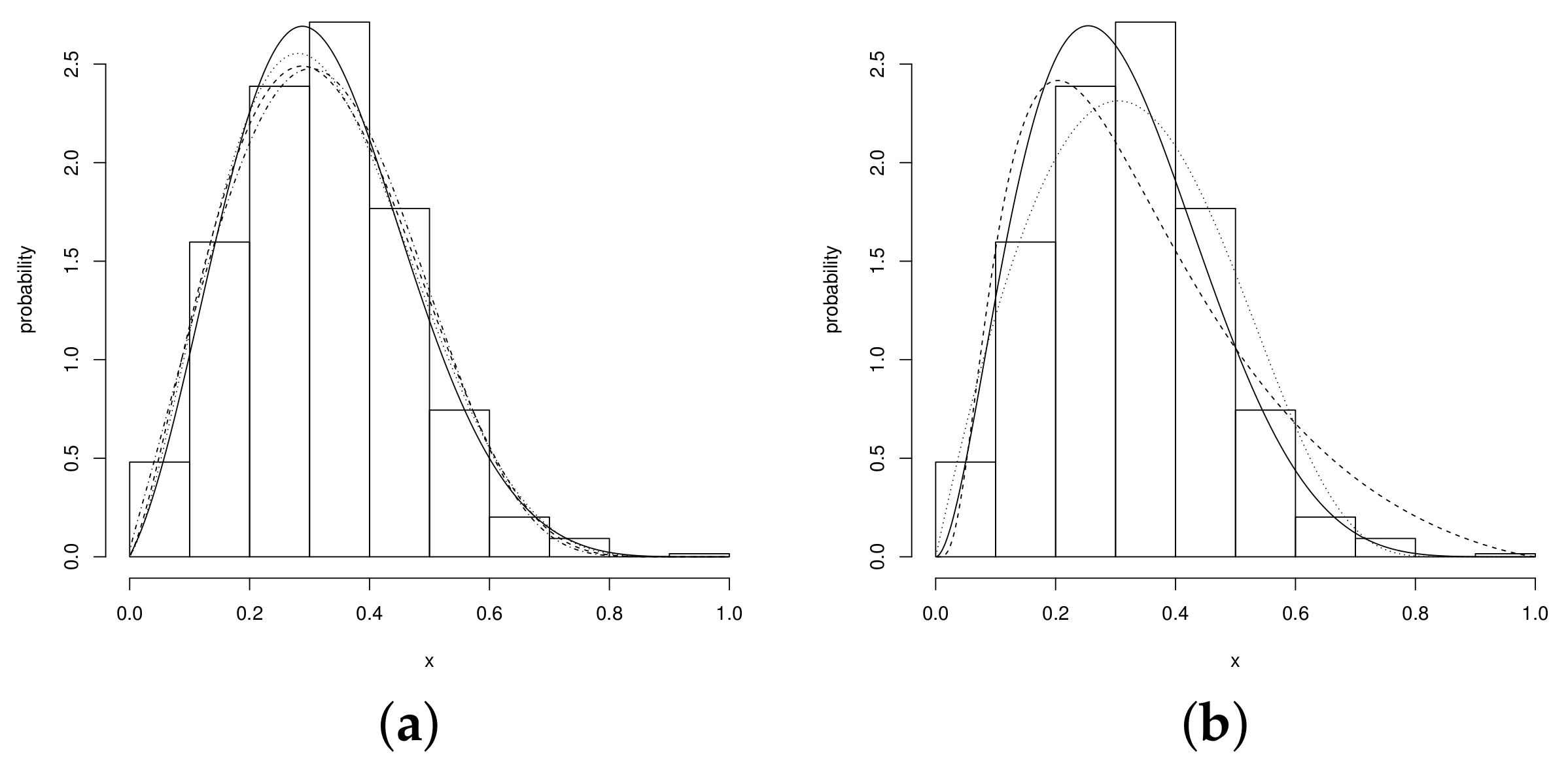
The Figure 3 shows the data set under analysis. To fit this set of observations we used the unit–Birnbaum–Saunder (UBS) and unit–Weibull (UW) distributions (see Mazucheli [5], Mazucheli et al. [6], respectively), the beta distribution and the proposed unit–power–skew–normal family, that is the UN, USN, UPN and UPSN distributions. The PDF of the fitted distribution are summarized in Table 4.

Figure 3.
Fitted distributions (a) UPSN (solid line), USN (dotted line), UPN (dashed line) and UN (dashed and dotted line), (b) Beta (solid line), UW (dotted line) and UBS (dashed line).
Table 4.
PDF of the distribution fitted to dataset.
To compare the distributions in question, we used the Akaike information criterion (AIC) of [24], the Bayesian information criterion (BIC) of [25], the AIC corrected (AICc) of [26] and the Hannan–Quinn information criterion by [27], defined respectively by
where p is the number of parameters of the model in question.
The ML estimates, with standard errors in parentheses, are given in the Table 5. According to the results shown by the AIC, AICc, BIC and HQC criteria, the two best distributions, those with the best fit, are the UPSN and beta distributions, respectively. The table also shows the results of the Anderson–Darling (AD) goodness-of-fit test statistic for the fitted models, with the respective p-Values in parentheses. Note that in particular in the UN, USN, UPN and UPSN distributions, the good fit hypothesis is not rejected.
Table 5.
Estimation of the parameters, with their standard errors, of the beta, UBS, UW, USN, UN, UPN and UPSN distributions.
We now compare the members of the UPSN family. We initially do the comparison of the UN distribution with the UPSN distribution by using the hypothesis test
with the likelihood ratio statistic,
we obtain
which is greater than the value . Then, the UPSN distribution is a good alternative for fitting the teacher set data. Now, for comparing the UPSN distribution with the UPN and USN distributions, we use the set of hypotheses
respectively, with the likelihood-ratio statistics
After numerical evaluations, we obtained
which is greater than the value . The best fitting, regarding the UN, UPN and USN distributions, is shown by the UPSN distribution. The graphs in Figure 3a,b show that the fitted distributions obtained from the estimates of the parameters of the UPSN distribution presents a better fit, compared to the UPN, beta, and UN distributions. Therefore, the graphs in the Figure 4a,b show the distribution function and the QQplot for the UPSN distribution, where the good fit of the UPSN distribution can be observed for the data set of teacher qualification of the basic level of teachers in the municipalities of Brazil. Likewise, the graphs in Figure 5 show the distribution functions of the remaining of the fitted models, in these it can be seen that the UN, USN and UPN distributions also fit the data set quite well, but the UPSN distribution fits much better. Making a Kolmogorov–Smirnov goodness-of-fit test, the statistic with p-Value = 0.8839 is obtained, which indicates that the fit of the UPSN distribution to the data set is good, as long as the fit for the beta distribution showed a value with p-Value = 0.1673, that is, the UPSN distribution better fits the data set of teacher qualification of the fundamental level of teachers in the municipalities of Brazil.
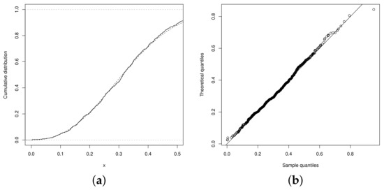
Figure 4.
(a) Empiric CDF (solid line) and UPSN distribution (dashed line), (b) QQplot UPSN distribution.
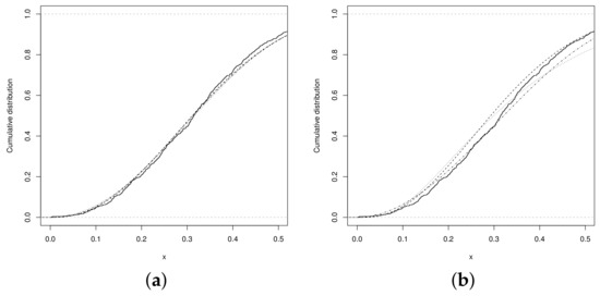
Figure 5.
CDF (a) USN (dashed line), UPN (dotted line) and UN (dashed and dotted line), (b) Beta (dashed line), UW (dotted line) and UBS (dashed and dotted line).
5.2. Model with Covariates
This data set was considered in Ferrari and Cribari-Neto [11], and it consists of family food expenses over 38 h taken from Griffiths et al. [28]. The data are available in the betareg library by Cribari-Neto and Zeileis [29] the R Development Core Team [22] software. The response or dependent variable is the quotient or tax , that is, the proportion of the family income spent on food, while the explanatory or independent variables are: the family income mentioned above and the number of people living at home. Ferrari and Cribari-Neto [11] fitted a beta regression model to explain the relationship between the response and the explanatory variables. For this data set, we fitted the following family of unit distributions: UN, USN, UPN and UPSN. The MLEs, with standard errors in parentheses, are given in Table 6. According to the results shown by the AIC, AICc, BIC and HQC criteria, the three regression models that present the best fit for the data are beta, UPN and UPSN, respectively. According to the AIC and BIC criteria, the UPSN regression model presents the best fit, followed by the UPN and the beta regression model, in that order.
Table 6.
Estimations of the parameters, with their standard errors, of the regression models beta, UN, USN, UPN and UPSN.
The UN regression model was compared with the UPSN regression model by using the hypothesis tests
Using the likelihood-ratio statistic:
we obtainied
which is greater than the value . Then, the UPSN regression model is a good alternative for fitting the data set. The UPSN regression model is also compared with the UPN regression model and the USN regression models by using the hypothesis tests
respectively, using the likelihood-ratio statistics:
After numerical evaluations, we obtained
which is greater than the value of the . The best fitting, with respect to the other models, is shown by the UPSN regression model.
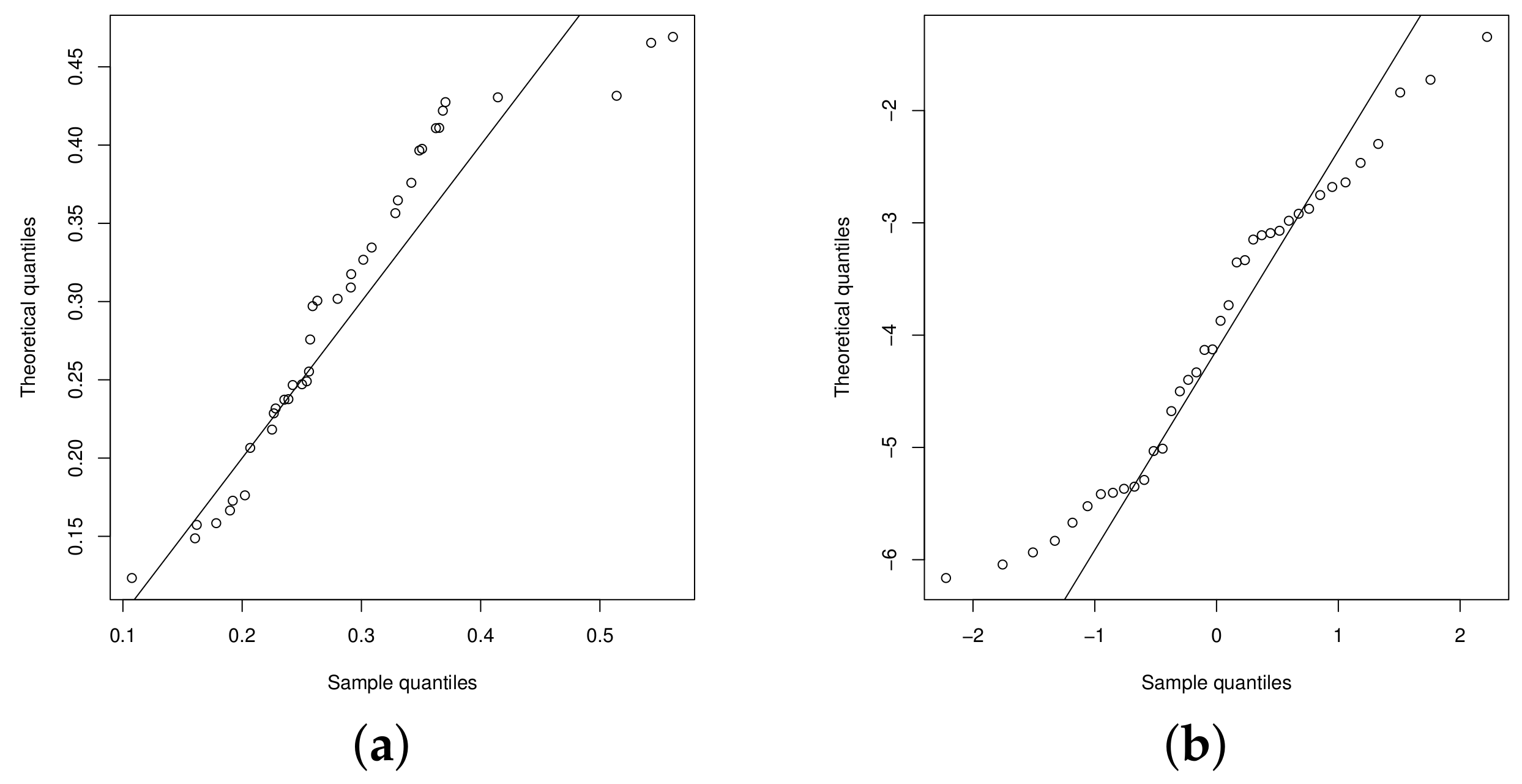
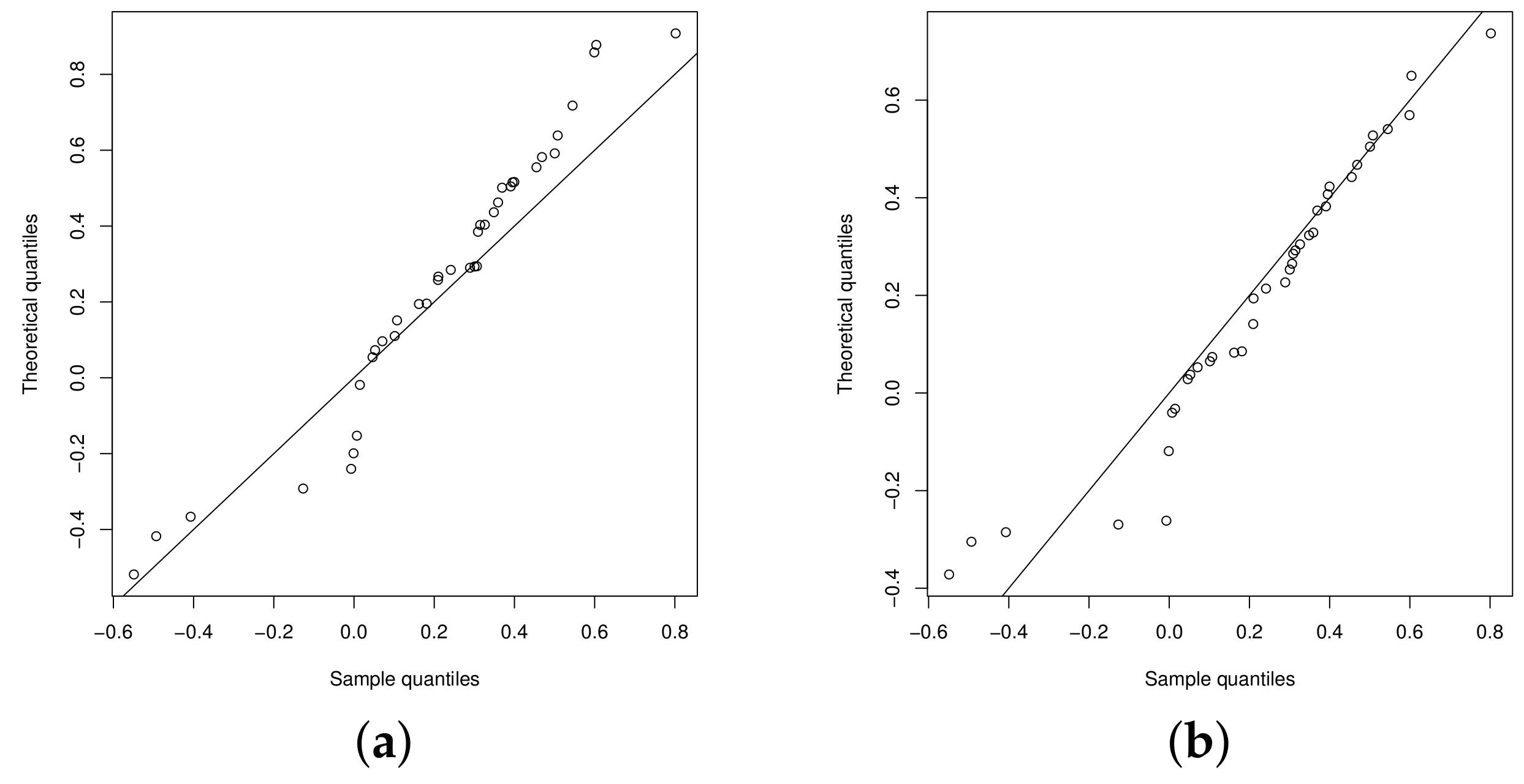
The QQplots of the statistic for the beta regression model and UN regression model are presented in the Figure 6a,b, respectively. Figure 7a,b show the QQplots for the UPN and UPSN regression models. From these figures, it can be noted that the UPSN regression model presents a better fit, compared to the UPN, beta and UN regression models.
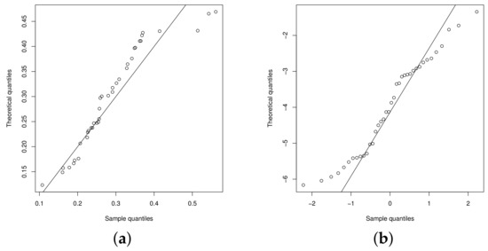
Figure 6.
QQplot: (a) beta regression model and (b) UN regression model.
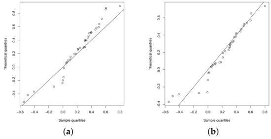
Figure 7.
QQplot: (a) UPN regression model and (b) USPN regression model.
We analyzed the transformed martingale residual by Barros et al. [30] given by
where is the martingal residual proposed introducen by Ortega et al. [31], where indicate whether the ith observation is censored or not, respectively, denotes the sign of and represents the survival function evaluated at (the standardized classical residuals), where being the MLE for . This analysis allows to identify atypical observations and/or model misspecification. To verify the assumptions of the model, the distribution of errors, adjustment problems and the presence of possible outliers, we generate confidence bands through simulations for the residual martingale, known in the literature of diagnostic analysis as envelopes.
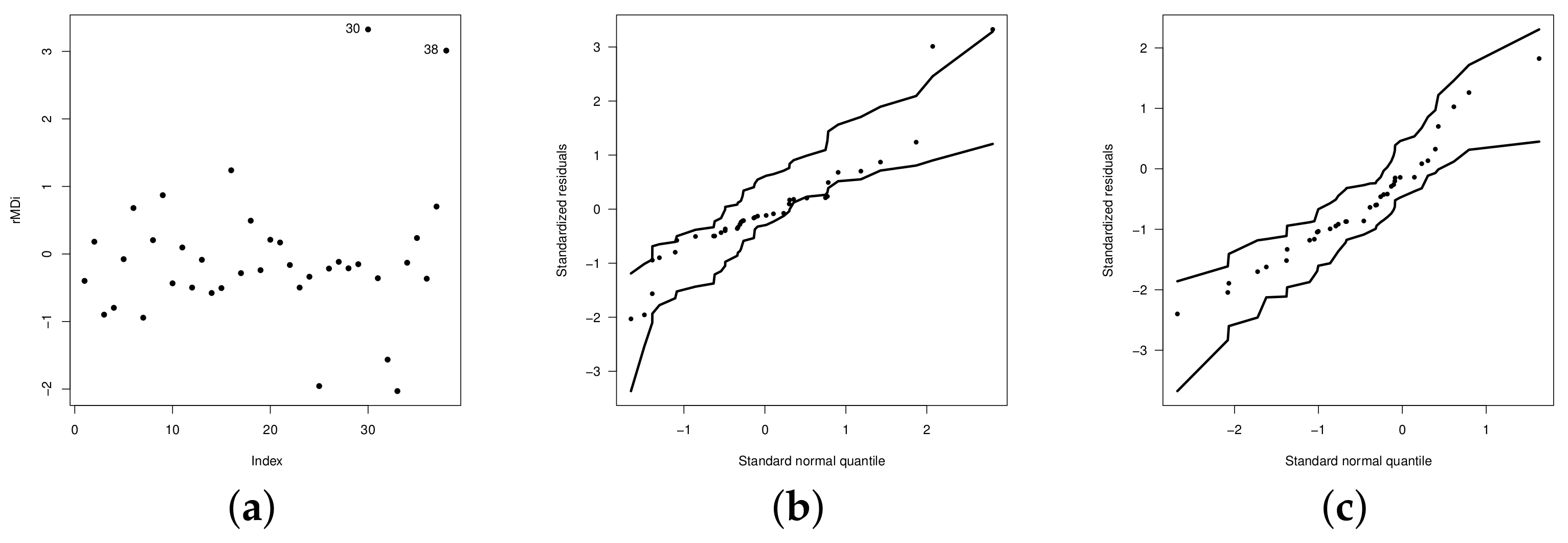
Figure 8a,b show the graphs of the residuals and the respective envelope, where some atypical observations can be observed (see observations and ). We remove these observations and again fit the regression model (see Figure 8c). Table 7 shows the estimates of the model parameters (with standard errors in parentheses) without outliers, while Table 8 shows the comparison criteria (log-likelihood, AIC, BIC, AICC and HQC) and the Shapiro–Wilk, Kolmogorov–Smirnov and Anderson–Darling good fit tests (with p-Values in parentheses) for the model residuals.

Figure 8.
(a) Plots of the residuals for the UPSN regression model. Envelope for the UPSN regression model with outliers (b), and without outliers (c).
Table 7.
Estimations of the parameters, with their standard errors, of the regression model UPSN.
Table 8.
Comparison criteria and Shapiro–Wilk, Kolmogorov–Smirnov and Anderson–Darling normality test.
Figure 8c shows the envelope plot of the martingale residuals for the fitted model without outliers, in which a good fit of the corrected model is observed.
6. Bivariate Extension of the UPSN Distribution
In this section, we explore and present some preliminary results of the extension to the bivariate case of the UPSN distribution. These previous results can be extended to the case of regression models for bivariate proportion data, being able to be a viable alternative to existing methods such as the one proposed by Lemonte and Moreno-Arenas [32].
Let us suppose a vector on the Cartesian plane. For the construction of the bivariate extension of the UPSN distribution, the methodology of conditionally specified distributions given by Arnold et al. [33] and Arnold et al. [34] is used. Thus, a bivariate vector is conditionally specified, if for any random variable , the conditional distribution of the random variable belongs to some parametric family of distributions. Thus, assuming that the random variables and are members of the family of the univariate UPSN distributions, that is,
and
where and are unknown positive dependency functions to be determined, namely,
and
where is the CDF of the SN distribution. Letting for the marginal densities, then the joint PDF is given by
Following Arnold’s Theorems in [34], according to Martínez et al. [35], applying Suto’s Theorem for the alpha-power family, the dependency functions have the form:
and
where are positive constants and is a dependence parameter.
So, using the Theorems given in Arnold and Strauss [36] and Arnold et al. [34], we arrive at the joint PDF of the bivariate vector which can be written as:
where for is defined in (4). We denoted it by Note that, implies
that is, independence between and . Thus, the conditional density functions can be written as:
and
Then, the marginal density functions have the form
and
For the estimation of the parameters of the BUPSN distribution, we do not use maximum likelihood due to the proportionality constant involved in the distribution, which makes it difficult to estimate the parameters with the double integral involved in this process. It is proposed to use the method of maximum pseudo-likelihood, based on conditional density functions. Thus, for the parameter vector the pseudo-likelihood is given by
Then, the maximum pseudo-likelihood estimators are given by the maximization of the log-pseudo-likelihood function given by
where , for is the log-likelihood function of the univariate UPSN distribution with parameters The MLEp can be obtained by equating to zero the pseudo-score function,
and solving this system of non-linear equations. According to Arnold and Strauss [36], the MLEP are consistent and asymptotically normal with asymptotic covariance matrix where:
where and
7. Conclusions
This article presents a distribution based on the skew–normal–power (PSN) distribution to fit proportions and rates on the unit interval as an alternative not only to the beta distribution, but also to other distributions that have been studied recently, such as unit–Lindley, unit–Weibull and unit–Birnbaum–Saunders. The unit–PSN or UPSN distribution is extended by adding covariates that explain the response variable. The estimating process of the parameters of the proposed distribution is presented for both cases, with and without covariates. The observed and expected information matrices are also addressed. The UPSN distribution showed great flexibility to model taxes and proportions in important practical scenarios. The introduced model presented a better fit than those beta and unit–Weibull, unit–Birnbaum–Saunder and unit–Lindley distributions in the case without covariates. Aditionally, UPSN showed better results than the beta regression model in the case with covariates.
Author Contributions
Conceptualization, G.M.-F.; Data curation, G.M.-F. and R.B.A.-F.; Formal analysis, G.M.-F., R.B.A.-F. and R.T.-F.; Funding acquisition, R.T.-F.; Investigation, G.M.-F. and R.B.A.-F.; Methodology, G.M.-F., R.B.A.-F. and R.T.-F.; Project administration, R.T.-F.; Resources, R.T.-F.; Software, G.M.-F. and R.B.A.-F.; Supervision, G.M.-F. and R.B.A.-F.; Visualization, R.B.A.-F. and R.T.-F.; Writing—original draft, G.M.-F. and R.T.-F.; Writing—review & editing, G.M.-F., R.B.A.-F. and R.T.-F. All authors have read and agreed to the published version of the manuscript.
Funding
The research of G. Martínez-Flórez and R. Tovar-Falón was supported by project: Resolución de Problemas de Situaciones Reales Usando Análisis Estadístico a través del Modelamiento Multidimensional de Tasas y Proporciones; Esquemas de Monitoreamiento para Datos Asimétricos no Normales y una Estrategia Didáctica para el Desarrollo del Pensamiento Lógico-Matemático. Universidad de Córdoba, Colombia, Acta de Compromiso FCB-05-19.
Institutional Review Board Statement
Not applicable.
Informed Consent Statement
Not applicable.
Data Availability Statement
Details about data available are given in Section 5.
Acknowledgments
G. Martínez-Flórez and R. Tovar-Falón acknowledge the support given by Universidad de Córdoba, Montería, Colombia.
Conflicts of Interest
The authors declare no conflict of interest.
Appendix A. Elements of the Observed Information Matrix
In this section, the elements of the observed information matrix for the USPN regression model are presented. They were obtained from the Formula (10).
where :
References
- Azzalini, A. A class of distributions which includes the normal ones. Scand. J. Stat. 1985, 12, 171–178. [Google Scholar]
- Durrans, S.R. Distributions of fractional order statistics in hydrology. Water Resour. Res. 1992, 28, 1649–1655. [Google Scholar] [CrossRef]
- Pewsey, A.; Gómez, H.; Bolfarine, H. Likelihood-based inference for power distributions. Test 2012, 21, 775–789. [Google Scholar] [CrossRef]
- Martínez-Flórez, G.; Bolfarine, H.; Gómez, H.W. Power-models for proportions with zero/one excess. Appl. Math. Inf. Sci. 2012, 12, 293–303. [Google Scholar] [CrossRef]
- Mazucheli, J.; Menezes, A.F.B.; Ghitany, M.E. The unit-Weibull distribution and associated inference. J. Appl. Probab. Stat. 2018, 13, 1–22. [Google Scholar]
- Mazucheli, J.; Menezes, A.; Dey, S. The unit-Birnbaum-Saunders distribution with applications. Chil. J. Stat. 2018, 9, 47–57. [Google Scholar]
- Mazucheli, J.; Menezes, A.F.B.; Chakraborty, S. On the one parameter unit-Lindley distribution and its associated regression model for proportion data. J. Appl. Stat. 2019, 49, 700–714. [Google Scholar] [CrossRef]
- Bhatti, F.A.; Ali, A.; Hamedani, G.; Korkmaz, M.Ç.; Ahmad, M. The unit Generalized Log Burr XII Distribution: Properties and Application. In Mathematical and Statistical Science Faculty Research and Publications; 2021; Volume 81, Available online: https://epublications.marquette.edu/math_fac/81 (accessed on 25 July 2022).
- Korkmaz, M.Ç.; Korkmaz, Z.S. The unit log–log distribution: A new unit distribution with alternative quantile regression modeling and educational measurements applications. J. Appl. Stat. 2021, 1–20. [Google Scholar] [CrossRef]
- Korkmaz, M.Ç.; Chesneau, C.; Korkmaz, Z.S. The Unit Folded Normal Distribution: A New Unit Probability Distribution with the Estimation Procedures, Quantile Regression Modeling and Educational Attainment Applications. J. Reliab. Stat. Stud. 2022, 15, 165–186. [Google Scholar] [CrossRef]
- Ferrari, S.; Cribari-Neto, F. Beta regression for modelling rates and proportions. Appl. Stat. 2004, 31, 799–815. [Google Scholar] [CrossRef]
- Ospina, R.; Ferrari, S.L.P. A general class of zero-or-one inflated beta regression models. Comput. Stat. Data Anal. 2012, 56, 1609–1623. [Google Scholar] [CrossRef]
- Martínez-Flórez, G.; Bolfarine, H.; Gómez, H.W. Doubly censored power-normal regression models with inflation. Test 2014, 24, 265–286. [Google Scholar] [CrossRef]
- Korkmaz, M.Ç.; Chesneau, C.; Korkmaz, Z.S. A new alternative quantile regression model for the bounded response with educational measurements applications of OECD countries. J. Appl. Stat. 2021, 1–24. [Google Scholar] [CrossRef]
- Mazucheli, J.; Alves, B.; Korkmaz, M.Ç.; Leiva, V. Vasicek Quantile and Mean Regression Models for Bounded Data: New Formulation, Mathematical Derivations, and Numerical Applications. Mathematics 2022, 10, 1389. [Google Scholar] [CrossRef]
- Mazucheli, J.; Korkmaz, M.Ç.; Menezes, A.F.B.; Leiva, V. The unit generalized half-normal quantile regression model: Formulation, estimation, diagnostics, and numerical applications. Soft Comput. 2022, 1–17. [Google Scholar] [CrossRef] [PubMed]
- Owen, D.B. Tables for computing bi-variate normal probabilities. Ann. Math. Stat. 1956, 27, 1075–1090. [Google Scholar] [CrossRef]
- Salinas, H.S.; Gómez, H.W.; Martínez-Flórez, G.; Bolfarine, H. Skew-normal alpha-power model [Statistics 48(2014) 1414–1428]. Statistics 2018, 52, 950–953. [Google Scholar] [CrossRef]
- Kundu, D.; Gupta, R.D. Power-normal distribution. Statistics 2013, 47, 110–125. [Google Scholar] [CrossRef]
- Martínez-Flórez, G.; Tovar-Falón, R.; Elal-Olivero, D. Some new flexible classes of normal distribution for fitting multimodal data. Statistics 2022, 56, 182–205. [Google Scholar] [CrossRef]
- Henningsen, A.; Toomet, O. maxLik: A package for maximum likelihood estimation in R. Comput. Stat. 2011, 26, 443–458. [Google Scholar] [CrossRef]
- R Development Core Team. R: A Language and Environment for Statistical Computing; R Foundation for Statistical Computing: Vienna, Austria, 2019; Available online: http://www.R-project.org (accessed on 31 January 2022).
- Martínez-Flórez, G.; Bolfarine, H.; Gómez, H.W. The alpha–power tobit model. Commun. Stat. Theory Methods 2013, 42, 633–643. [Google Scholar] [CrossRef]
- Akaike, H. A new look at statistical model identification. IEEE Trans. Autom. Control 1974, AU-19, 716–722. [Google Scholar] [CrossRef]
- Schwarz, G. Estimating the dimension of a model. Ann. Stat. 1978, 6, 461–464. [Google Scholar] [CrossRef]
- Schwarz, G. Further analysis of the data by akaike’s information criterion and the finite corrections. Commun. Stat. Theory Methods 1978, 7, 13–26. [Google Scholar]
- Hannan, E.J.; Quinn, B.G. The Determination of the order of an autoregression. J. R. Stat. Soc. Ser. B 1979, 41, 190–195. [Google Scholar] [CrossRef]
- Griffiths, W.E.; Hill, R.C.; Judge, G.G. Learning and Practicing Econometrics; Wiley: New York, NY, USA, 1993. [Google Scholar]
- Cribari-Neto, F.; Zeileis, A. Beta Regression in R. J. Stat. Softw. 2010, 34, 1–24. Available online: https://www.jstatsoft.org/article/view/v034i02 (accessed on 31 January 2022). [CrossRef]
- Barros, M.; Galea, M.; González, M.; Leiva, V. Influence diagnostics in the tobit censored response model. Stat. Methods Appl. 2010, 19, 379–397. [Google Scholar] [CrossRef]
- Ortega, E.M.; Bolfarine, H.; Paulda, G.A. Influence diagnostics in generalized log-gamma regression models. Comput. Stat. Data Anal. 2003, 42, 165–186. [Google Scholar] [CrossRef]
- Lemonte, A.J.; Moreno-Arenas, G. On a multivariate regression model for rates and proportions. J. Appl. Stat. 2019, 46, 1084–1106. [Google Scholar] [CrossRef]
- Arnold, B.C.; Castillo, E.; Sarabia, J.M. Conditionally specified distributions. In Lecture Notes in Statistics; Berger, J., Fienberg, J., Gani, J., Krickeberg, I., Singer, B., Eds.; Springer: New York, NY, USA, 1992; Volume 73. [Google Scholar]
- Arnold, B.C.; Castillo, E.; Sarabia, J.M. Conditionally Specification of Statistical Models; Springer Series in Statistics; Springer: New York, NY, USA, 1999. [Google Scholar]
- Martínez-Flórez, G.; Arnold, B.C.; Bolfarine, H.; Gómez, H.W. The multivariate alpha-power model. J. Stat. Plan. Inference 2013, 143, 1244–1255. [Google Scholar] [CrossRef]
- Arnold, B.C.; Strauss, D. Bivariate distributions with conditionals in prescribed exponential families. J. R. Stat. Soc. Ser. B 1991, 53, 365–375. [Google Scholar] [CrossRef]


Publisher’s Note: MDPI stays neutral with regard to jurisdictional claims in published maps and institutional affiliations. |
© 2022 by the authors. Licensee MDPI, Basel, Switzerland. This article is an open access article distributed under the terms and conditions of the Creative Commons Attribution (CC BY) license (https://creativecommons.org/licenses/by/4.0/).