Abstract
This paper proposes a novel hybrid optimization technique based on a machine learning (ML) approach and transient search optimization (TSO) to solve the optimal power flow problem. First, the study aims at developing and evaluating the proposed hybrid ML-TSO algorithm. To do so, the optimization technique is implemented to solve the classical optimal power flow problem (OPF), with an objective function formulated to minimize the total generation costs. Second, the hybrid ML-TSO is adapted to solve the probabilistic OPF problem by studying the impact of the unavoidable uncertainty of renewable energy sources (solar photovoltaic and wind turbines) and time-varying load profiles on the generation costs. The evaluation of the proposed solution method is examined and validated on IEEE 57-bus and 118-bus standard systems. The simulation results and comparisons confirmed the robustness and applicability of the proposed hybrid ML-TSO algorithm in solving the classical and probabilistic OPF problems. Meanwhile, a significant reduction in the generation costs is attained upon the integration of the solar and wind sources into the investigated power systems.
MSC:
90C26
1. Introduction
The optimal power flow (OPF) problem is classified as a nonlinear optimization problem, and it can be used as a power system tool that aims to determine the best possible values for the decision variables corresponding to the objective functions, satisfying the system constraints [1,2]. In the last decade, several approaches to solutions have been presented in the literature to solve the OPF problem, as reviewed in detail in [3,4]. In the same vein, different objective functions are studied by the researchers, such as the minimization of the generators’ real power costs, daily operational costs, production emission rate, and power losses [5,6]. However, an optimal decision for the dispatchable distributed generation units has not yet been achieved [7]. Previously, deterministic approaches were used to solve the classical OPF problem without integrating renewable energy sources (RESs) [8]. Motivated by the ambitious new climate change policies and regulatory schemes that encourage the diversification of energy sources for energy security and carbon emission mitigation purposes, the high penetration of RESs into grids has been promoted [9,10]. However, this results in uncertainties and parameters’ statistical changes [11,12]. Consequently, the probabilistic power flow (PPF) [13,14] or probabilistic OPF (POPF) problems should be solved from a probabilistic point of view rather than the traditional deterministic approaches, as reviewed in detail by Ramadhani et al. [15] and Prusty and Jena [16,17]. The stochastic variations in wind speed and solar irradiance are the motivation for researchers to seek sophisticated statistical models for simulating solar and wind power generation.
The major classifications of PPF problem solution methods are subject to the analytical, approximate, numerical, and heuristic methods classified in the large reviews [18,19]. In the analytical method, the equation is obtained between the input and the output and then calculated directly from the input variables. For example, [20] proposed a data-driven approach for probabilistic forecasts of the distribution grid state and PPF solution. Ref. [21] developed a fast-specialized point estimate method compared to the Monte Carlo simulation (MCS) approach to solve the POPF considering the IEEE-69 bus distribution system with the presence of RESs. Ref. [22] presented a clustering-based analytical method for PPF and interval power flow, in which the uncertainties of load demands and wind power outputs were adequately handled. Ref. [23] introduced a new framework based on the relevance vector machine (RVM) compared to the Newton–Raphson method in order to calculate the PPF and the multivariate distribution of wind speed considering uncertainties associated with multi-dimensional wind turbine (WT) farms studying the correlation between wind speed in different regions. The linearization in the analytical method makes the power flow calculations simpler; however, the accuracy of the PPF problem solution is poor. The approximate method computes the moments of the output using the PDF of the input variables. Despite successfully solving the PPF problem without large-scale computations, the computation burden increases as the number of stochastic variables increases. The third type, the MCS, is a frequently utilized numerical method for the solution of the PPF problem [24]. The MCS is a more reliable method to solve the PPF problem. According to the recent review by Skolfield and Escobedo [19], the advancements in metaheuristic algorithms for power system applications have proven to have superior advantages compared to methods in solving the classical and stochastic OPF [18].
Considering the scope of the current study, the review analysis only focuses on the most recent studies on PPF or POPF. For example, [25] presented differential evolutionary particle swarm optimization to solve the multiple objectives (fuel cost, emission, and prohibited operating zones of thermal generators) POPF problem, in which the uncertain solar irradiance and wind speed were simulated via log-normal and Rayleigh probability distributions validated for IEEE 30, 57, and 118 test systems. Ref. [26] proposed a novel barnacles mating optimizer (BMO) to solve the POPF with stochastic solar power to minimize either the generation cost, power loss, voltage deviation, emission minimization, or combined cost and emission of power generations of the IEEE-30 bus system. Similarly, the BMO algorithm was used by [27], while the study incorporated the stochastic small hydro power generator plus wind and solar. Ref. [28] developed a hybrid algorithm that combines the Moth Swarm Algorithm (MSA) and the Gravitational Search Algorithm (GSA) with the Weibull Distribution Function (WDF) used to demonstrate the alternating nature of wind farms integrated with the studied power systems. Moreover, [29] introduced a hybrid methodology based on the differential evolution (AGDE) algorithm and the Fitness–Distance Balance (FDB) method to solve the POPF involving wind and solar energy systems with the IEEE 30-bus test system. Ref. [30] developed a combination of phasor particle swarm optimization and a gravitational search algorithm—namely, a hybrid PPSOGSA algorithm—to calculate the POPF in the case of the IEEE 30-bus system, considering the forecasted WT and PV power generation as uncertain variables. Most recently, Ref. [31] came up with a novel algorithm called the Heap Optimization Algorithm (HEAP) for OPF solutions when solar and wind generators are added. The method was validated with three standard systems (IEEE 30, 57, and 118) and compared with a genetic algorithm. Ref. [32] solved the POPF problem for the modified IEEE-39 bus system while incorporating the uncertainty-related expense incurred due to the stochastic behavior of PV and WT generation, in which the solar radiation and wind speed are modelled using WPD and normal distributions and the uncertainty is simulated using the MCS method. Ref. [33] employed a hybrid Point Estimate Method (PEM)/Ant Lion Optimization (MALO) approach for handling loads, wind, and solar uncertainties and solving the POPF with multiple objectives in the case of a modified IEEE 33-bus islanded micro-grid system. Ref. [34] developed a general computationally efficient copula-polynomial chaos expansion to solve PPF, including both linear and nonlinear relations of stochastic wind and PV power generation. Rosenblatt transformation is employed to convert the correlated variables and obtain independent variables, keeping in mind the dependence structure. The systems used are the IEEE 57- and 118-bus systems. Ref. [35] presents the PPF problem solution based on a scaled unscented transformation. The PPF problem is applied on AC/DC networks. It is applied on the modified IEEE 1354-bus (PEGASE) system. Ref. [36] introduces a PPF problem solution including hundreds of uncertain variables. The Zhao’s point estimate technique is used when solving the PPF problem. As the number of PPF problem inputs increases, the computational burden increases linearly. The studied cases are investigated on a modified IEEE 118-bus system. Ref. [37] presents a comparative analysis of Monte Carlo simulation with the Latin Hypercube sampling method and Unscented transformation methods. The comparisons are with the results achieved by the classical Monte Carlo simulation method. The test systems used are the IEEE 14- and 30- bus systems. The results confirm the superiority of the unscented transformation method in terms of speed and reliability over the other two methods. Table 1 summarizes the optimization methods used in this literature.

Table 1.
Summary of some of the references stated in the literature.
This paper introduces a new hybridization of the self-organizing maps (SOM) machine learning technique and the transient search optimization (TSO) algorithm. The ML provides the systems with the ability to understand themselves and then estimate unknown outputs [38,39]. The SOM technique is considered one of the important artificial neural network (ANN) architectures and features the ability for data visualization processing. It is classified as an unsupervised ANN and is utilized for knowledge extraction in order to determine the best areas with the objective of reducing the exploration field. The TSO algorithm was first proposed in 2020 by Qais, Hasanien, and Alghuwainem [38,40] and was inspired by the transient behavior of the first- and second-order circuits, which include energy storage elements (e.g., inductors and/or capacitors). Using the ML-TSO in optimization, one reaches the global solution efficiently without being stuck in a local solution. The main contributions of this paper are as follows:
- Proposing a novel hybrid optimization approach based on the ML technique and TSO algorithm—namely, ML-TSO—for the optimal solution of classic OPF and POPF problems.
- Formulating the ML-TSO algorithm to consider the integration of both conventional generators, renewable sources (PV panels and WTs), and time-varying load profiles.
- Introducing the statistical models for the PV panels and WTs using the Beta and Weibull distribution functions based on real-time historical data. This allows us to calculate the generated electrical power RESs accurately while solving the PPF problem.
- Validating the robustness of the proposed hybrid algorithm, built in MATLAB software, on the IEEE 57-and 118-bus test systems, with comparative analysis with the most recent literature.
The rest of the paper is organized in the following sections as follows: the problem formulation is illustrated in Section 2; the modeling of WT and PV generation systems is presented in Section 3; Section 4 describes the proposed hybrid ML-TSO algorithm. The simulation results are demonstrated in Section 5; and, finally, the paper is concluded in Section 6.
2. Problem Formulation
Considering the study objectives, the proposed hybrid ML-TSO optimization algorithm is first implemented to solve the classical OPF, with the objective function formulated to minimize the total generation costs. For a realistic solution of the POPF problem, the algorithm structure is adapted to consider the unavoidable uncertainty of solar PV and WT generators and time-varying load profiles.
2.1. The Classical OPF Problem
In this analysis, the OPF is solved for the IEEE 57 and 118 systems with fixed demand and conventional generations only. The objective function as well as the constraints of the problem are explained more in the following subsections.
2.1.1. The Objective Function
Herein, the objective function is formulated as the summation of the total costs of the power generated by the conventional generators. The defined cost function is a quadratic function of the active generated powers in the system. It is mathematically expressed in Equations (1) and (2) [41].
where represents the objective function, which is the summation of the power generation cost. refers to the number of the conventional generators in the system under study. refers to the power generated from the generator at the bus number ‘’ at the hour ‘’. For part ‘B’ of the problem formulation, this objective function is recalculated hourly with ‘’ step 1.
2.1.2. The System Constraints
The OPF problem has equality constraints on the active and reactive power besides the thermal limits of the transmission lines, as expressed in Equations (3), (4), and (8). There are inequality constraints representing the limits on the active and reactive power of each generator, in addition to the bus voltage constraints given in Equations (5)–(7) [41].
where and represent the power injection into the bus ‘’. In part ‘B’ of the problem formulation, when the OPF is repeated hourly, the symbol ‘’ refers to the hour at which the simulation is run. The symbols and represent the voltages of bus ‘’ and bus ‘’. Additionally, the symbol ‘’ refers to the hour during the day when the simulation is run. refers to the conductance. Meanwhile, refers to the susceptance. The is the voltage angle of bus ‘’. The is the voltage angle of bus ‘’. Additionally, ‘’ is the simulation hour at part ‘B’.
where is the minimum allowable active power that can be generated from the generator number ‘’. Meanwhile, is the maximum active power that can be generated from the ‘’th generator. is the minimum allowable reactive power of the ‘’th generator. Meanwhile, is the maximum reactive power of the ‘’th generator. denotes the thermal limit of the transmission line between buses ‘’ and ‘’.
2.2. OPF with RES Considering the Uncertainty (Probabilistic OPF Problem)
The OPF formulation is adapted to consider the unavoidable uncertainty of solar PV and WT generators and time-varying load profiles [42,43]. For an extensive analysis, the four different cases of the OPF problem are constructed and solved (i) case 1: the load is changing hourly through the day, and there is no RESs integrated into the system; (ii) case 2: the load is changing hourly through the day, and PV is integrated into the system; (iii) case 3: the load is changing hourly through the day, and WT is integrated into the system; (iv) case 4: the load is changing hourly through the day, and both solar PV and WT are integrated into the system. All these cases of OPF are studied to investigate how much the generation costs are changed by changing the load and by connecting renewable energy sources to the systems under study. The addition of the RESs increases the model complexity of the OPF problem.
In the later three cases with PV and/or WT integration, the output powers from these RESs are correctly modeled as non-dispatchable. To do so, the generation values from the PV and WT are applied to the system as forecasted values at certain preset buses, and they supply part of the systems’ demands. This correspondingly reduces the amount of electrical power generation needed from the conventional generators. The time interval of the repetition of the OPF solution is set to be one hour through a day. At every time interval ‘’ (1 h), there are 6 wind speed readings and 60 solar irradiance readings. The PV and the WT are assumed to generate only active power, and there is no reactive power generation. The forecasted power generation from the PV and WT sources are calculated according to probabilistic models of the wind speed and the solar irradiance, besides some technical characteristics of each source [31].
Using the MATLAB software and the built-in MATPOWER library, the classic OPF and POPF are solved. The computer used for this study is “lenovo ideapad 330 (15” Intel)”, whose CPU is “Up to 8th Gen Intel® Quad Core i7-8550U”. The proposed ML-TSO algorithm generates random solutions and guarantees that these suggested solutions have values between their maximum and minimum limits defined in Equation (5). The constraints defined in Equations (3), (4) and (6) are satisfied by the Newton–Raphson power flow. Moreover, penalties are inserted into the main objective function, defined in Equation (2), to eliminate any violation of limits that can happen to the other dependent variables and to consider this suggested solution as an infeasible one. These penalties are defined in Equation (9).
where and refer to predefined large positive numbers, and . refers to the apparent power of the branch number . Meanwhile, refers to the maximum value of the apparent power of the branch .
3. Modeling of the PV and WT Generation
In this paper, the integration of wind turbines and PV generation has been considered in the PPF problem solution. However, as we mentioned earlier, due to the RES power generation dependency on the metallurgical conditions, the power generation profile of the WT and PV is highly uncertain [44,45]. Therefore, it is important to accurately model the PV and WT generators as follows:
3.1. Modelling of PV Power Generation
The active power generated by the PV panel depends on the solar irradiance in (W/m2). It can be calculated as follows [29]:
where refers to the nominal power of the PV panel. represents the standard conditions’ solar irradiance. defines a certain irradiance point.
The solar irradiance is modelled by the Beta PDF as follows:
In Equation (11), is expressed in kW/m2. and are the shape parameters of the Beta PDF. is the Gamma function.
The parameters and are calculated using the mean and the standard deviation of the observations of the solar irradiance during a periodic time :
The Beta function is sampled to samples. The probabilistic solar irradiances, which correspond to the samples of the Beta PDF, are then used to calculate the forecasted values of active power generation from the PV panel as follows:
where represents the solar irradiance of the sample number g at hour . represents the irradiance probability of the sample number g at hour .
3.2. Modelling of WT Power Generation
The power generated by the wind turbine depends on the wind speed (). It can be calculated as follows [30]:
where represents the nominal wind turbine power. refers to the nominal speed of the wind. and are the cut-in and the cutoff wind speeds.
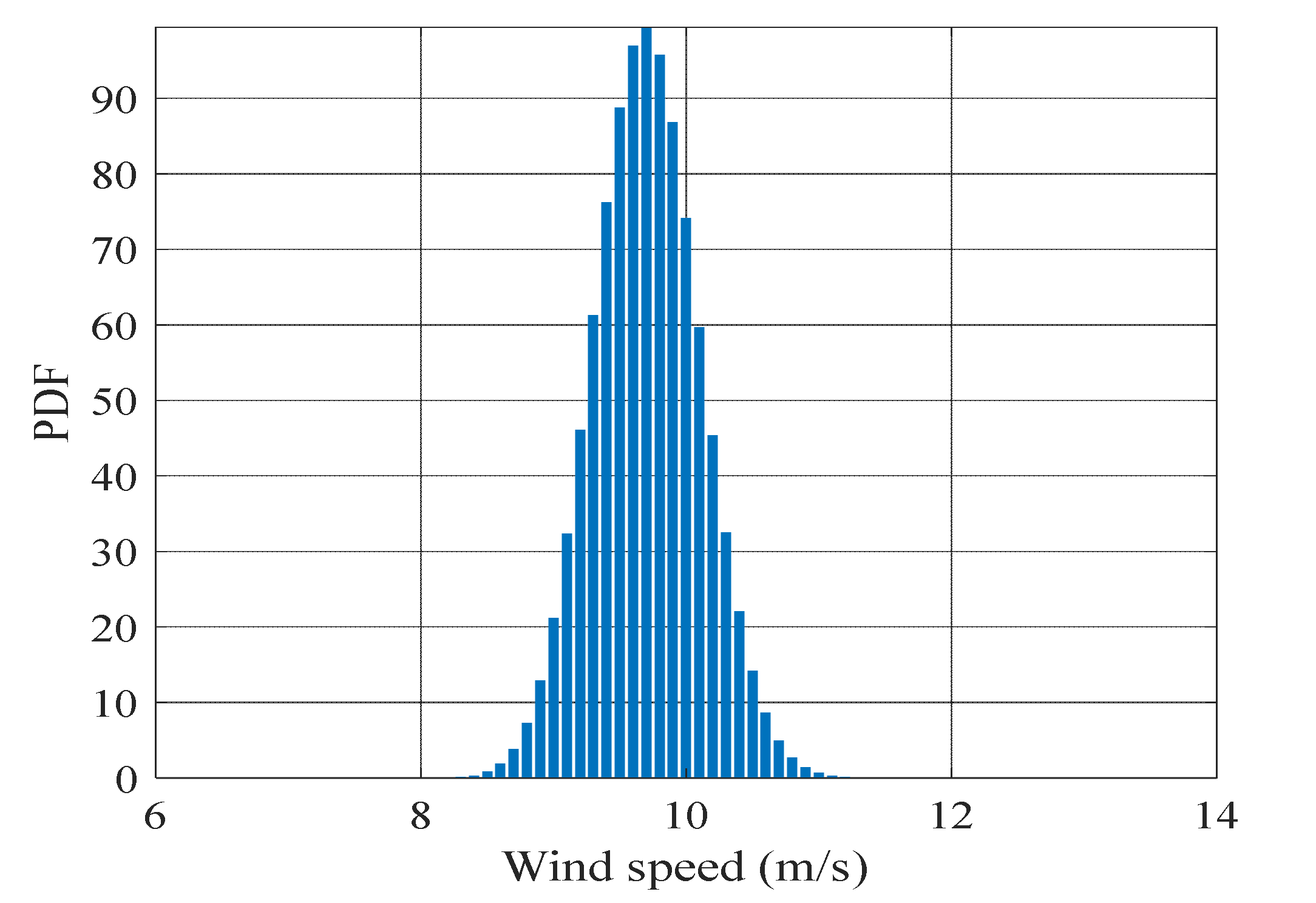
The wind speed is modelled by the Weibull PDF as follows:
where and represent the scale and shape parameters of the Weibull PDF. represents a uniform random which is distributed between 0 and 1.
The scale and shape parameters, and , are obtained from the mean and the standard deviation values of the wind speeds measured at hour ‘’ as follows:
The Weibull function is sampled to samples. The probabilistic wind speeds, which correspond to the samples of the Weibull PDF, are then used to calculate the forecasted values of active power generation from the wind turbine as follows:
where represents the wind speed of sample number g at hour . represents the wind speed probability of the sample number g at hour .
4. Proposed Solution Method
This paper proposes a new hybrid ML-TSO optimization algorithm in order to acquire the features of ML and TSO together and introduce an efficient tool for finding the optimal solutions for classic and POPF problems.
4.1. TSO Algorithm
The transient search optimization algorithm is inspired by the transient behavior of the circuits, which include energy storage elements in their configuration [46]. The transient behavior of the circuit depends on the circuit order, whether it is the first-order or second-order circuit. The circuit order can be determined by the number of energy storage elements, inductors, and capacitors in the circuit schematic. This overall transient behavior consists of transient and steady-state parts.
For the first-order circuits, the differential equation describing the transient behavior can be expressed as follows [46].
This equation can be solved for as a function of time as follows:
where represents the capacitor voltage or inductor current. τ is the time constant. is an initial condition-dependent constant. is the steady-state value.
The previous second-order differential equation can be solved as follows:
where is the damping coefficient and and are the resonant and damped frequencies. and refer to arbitrary constants.
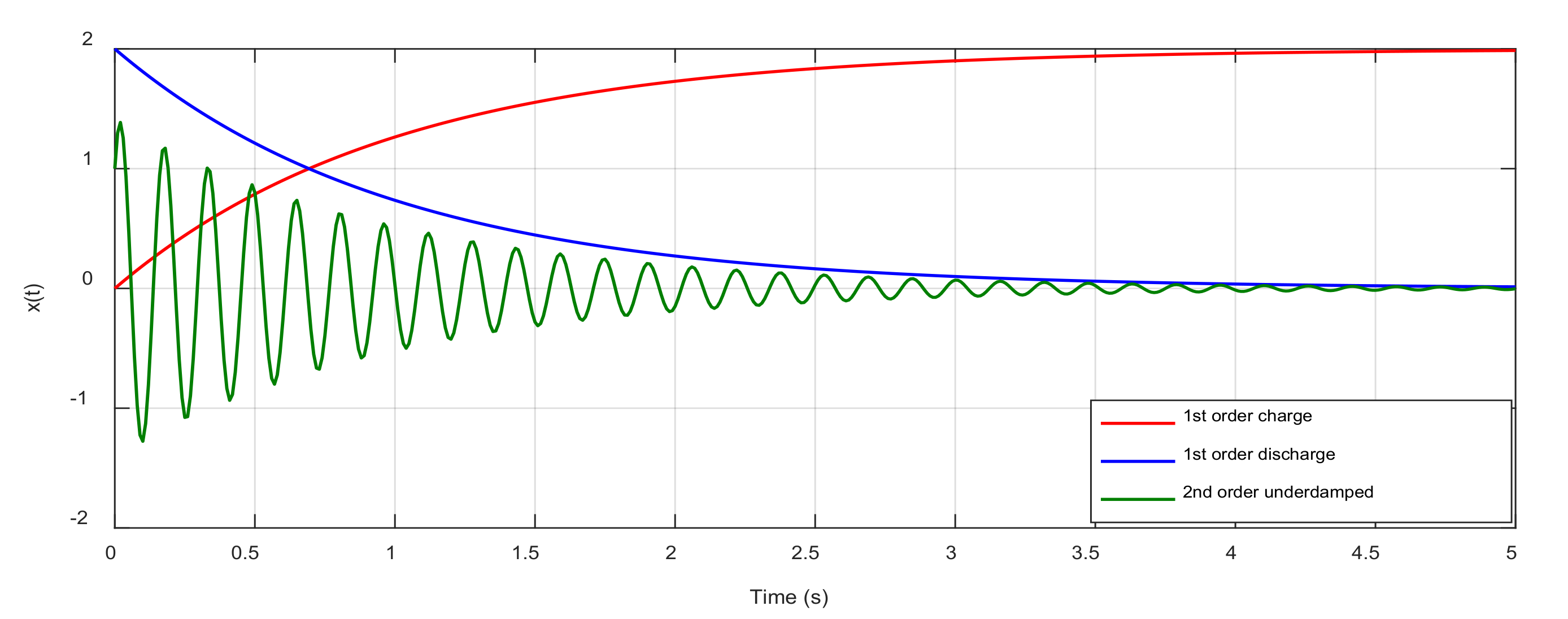
The responses of the circuits are graphically shown in Figure 1.
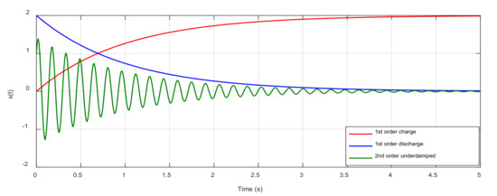
Figure 1.
Transient response of the circuits.
The TSO Inspiration
Similar to the other metaheuristic optimization algorithms, the first step in the TSO is to set random agents whose values lie between predefined boundaries according to the following equation [47]:
After that, it explores the optimal solution using the exploration and exploitation steps. The exploration step is inspired by the oscillatory response of the second-order circuits. Finally, it reaches the optimal solution after a predefined number of iterations. Moreover, the exploitation step is inspired by the exponential decay of the first-order circuits. Mathematically, the exploration and the exploitation steps can be expressed as follows:
where , , , , and refer to random numbers. and represent the population and the best population until the th iteration, respectively. refers to a counter that starts from 0. The stopping criterion is that when the iterations reach . corresponds to . Additionally, . ‘’ is a variable that lies between −2 and 2, which is used to balance the exploration and exploitation processes. The effect of changing ‘’ is shown in Figure 2. The pseudo-code of the TSO is provided in Algorithm 1.
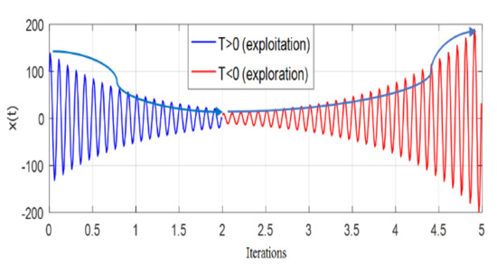
Figure 2.
Effect of the variable ‘’ on the exploration and exploitation processes.
| Algorithm 1. Pseudo code of the TSO algorithm. |
| Initialize the first population and obtain the best agents |
| Compute the fitness function |
| While the iteration number < the max. number of iterations |
| Use the Equations (26)–(28) to calculate T, C1, and a |
| Do for each population |
| Use the Equation (25) to calculate the Updated positions |
| End do |
| Obtain the fitness of the updated population |
| IF the new fitness is better than the best fitness Then |
| Replace the fitness and the population |
| End IF |
| l = l + 1 |
| end while |
| return Yl* |
Moreover, modifications to the existing TSO algorithm are made using the levy [48] and Weibull distribution functions [49], as described below.
4.2. Levy Function
Part of the population is modified using the levy function with the factor ‘’. It is expressed as follows:
where and are random numbers ranging from [0, 1].
4.3. Weibull Distribution Function
Another part of the population is modified using the Weibull distribution function with factor (). It is mathematically expressed as follows:
where and refer to the Weibull distribution constants whose values are 2 and 1, respectively.
The modified TSO populations, using the levy and Weibull distribution functions, are calculated as shown in (31). The population of the next iteration is updated by one of four equations according to a random number (). When is less than ‘0.25’, the population is modified using the levy function based on the current best population, the parameter ‘’, and the parameter ‘’. When is between ‘0.25’ and ‘0.5’, the population is modified using the Weibull function based on the current best population and . When is between ‘0.5’ and ‘0.75’, the population is modified using the Levy function based on the current best population and . Finally, when is greater than ‘0.75’, the population is modified using the Weibull function according to the current best population and .
where is a constant that is set to ‘0.5’ in this research. is a constant that depends on the number of current iterations and the maximum number of iterations. The is calculated as follows:
where ‘’ is the current population. ‘’ is the best population obtained until the current iteration. is the Weibull distribution function whose inputs are the dimension of the problem, the population size, and the location, shape, and scale parameters of the Weibull distribution. The location, shape, and scale parameters of the Weibull distribution are set to be 0, 2, and 1. ‘’ is the levy function, whose inputs are the dimension of the problem, the population size, and a constant set to ‘1.5’.
4.4. Machine Learning Approach
Self-organizing maps (SOMs) are considered important techniques in the machine learning approach [50]. SOMs can be classified as unsupervised neural networks that are utilized as a technique to extract the knowledge to determine the best areas to reduce the exploration field [51,52]. By using SOMs, multidimensional data can be analyzed. It has advantages over the other knowledge extraction methods such as preserving the organized data of the original elements as they are. Consequently, SOMs are commonly used as an approach for data reduction.
The SOM integrates two layers, where the first layer is called the input layer, and the second layer is named the competitive layer. The second layer involves a number of neural units ordered as a 2-D lattice. The construction of the SOM is shown in Figure 3.
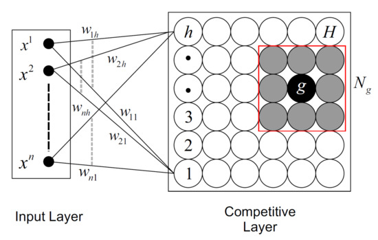
Figure 3.
Representation of a SOM.
The SOM has an output lattice of neural elements. The input is a vector of dimension . The data of vector are connected to each neural element. Every neural element lattice contains a weight vector with n units. The training of a SOM includes the weight adjustment and the neighborhood definition [50]. The learning steps contain two phases: the similarity calculation and the weight adaptation. First, the initial weights are small and random. After that, the initial vector of data is inserted into the neural network. Then, the weights of the neural elements are adapted. For more visualization to the effect of data-reduction and clustering, Figure 4 is provided [50].
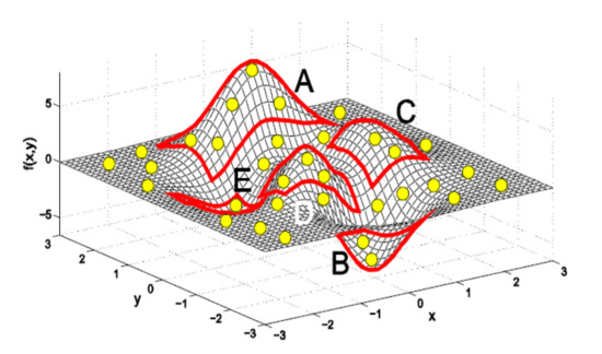
Figure 4.
Data reduction effect: Training process function.
4.5. Proposed Hybrid ML-TSO
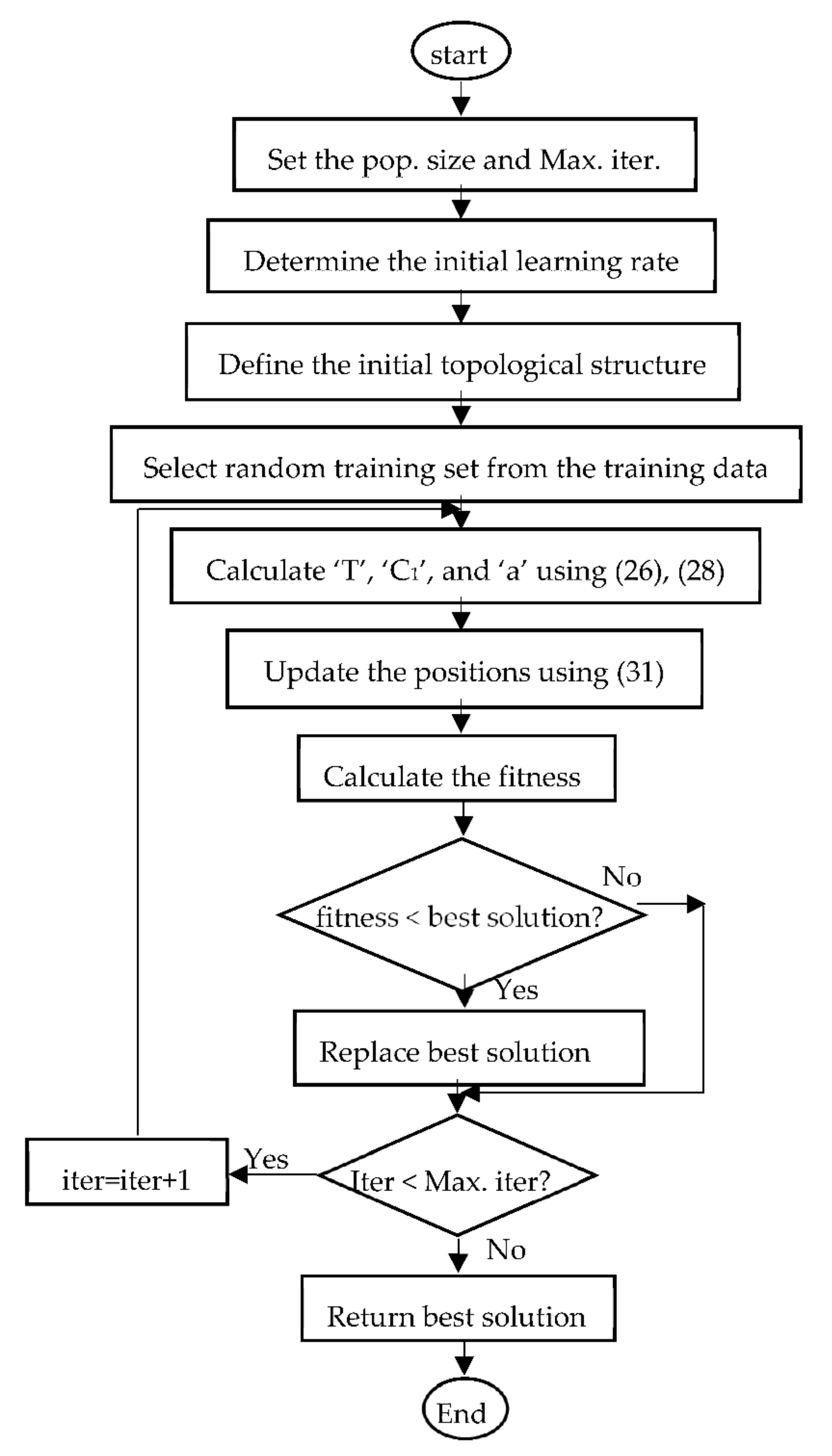
In this paper, a new hybridization between the modified version of the SOM and TSO was made. First, an initial random population is assumed. The machine learning part of the optimization code is applied. A small random value is assigned to all weights. The initial learning rate and topological structure are determined. A number of iterations for the learning process are set. After the training, an input vector is selected randomly from the training set. Define the winner neuron as the nearest to the input. Update the weights of the winner unit and neighboring ones. Then, the fitness function is calculated, and it converges to the best solution using the SOM. The populations are also updated correspondingly. The employment of the SOM before starting optimization using the TSO makes the convergence performance of the TSO more efficient. The population of the TSO is then modified and updated by the levy function and the Weibull distribution function. According to a random number, there are four possibilities to update the population. This process is repeated until the maximum number of iterations is reached. At every iteration, the best solution is obtained. The best solution is compared with the fitness calculated in the current iteration. If the fitness of the current iteration is better than the saved best solution, the fitness replaces the best solution. It should be mentioned that the metaheuristic optimization methods are significantly affected by the initialization process. The flow chart of the proposed hybrid ML-TSO algorithm is provided in Figure 5.

Figure 5.
The flowchart of the proposed algorithm.
5. Results and Discussion
In this section, the results and discussion of the main findings are comprehensively demonstrated by dividing them into three subsections. The first subsection presents the classical OPF problem. This subsection aims to examine, analyze, and evaluate the performance of the newly developed hybrid ML-TSO optimization method in solving the OPF problem compared to other methods in the existing literature. Furthermore, this subsection shows how applicable the ML-TSO method is in further optimization problems in the field of power systems. The test validation systems adopted in this study are the standard IEEE-57 bus and IEEE 118-bus test systems. The second subsection presents the simulation results of the POPF problem after integrating the RESs of PV and/or WT. The uncertainties caused by the random variability of the load demand and the stochastic behavior of the solar and wind power were adequately handled and modelled. This subsection also shows the effect of the RESs’ integration on the overall operating costs of the power system. The final subsection provides a statistical analysis of the numerical optimization results obtained for OPF in the case of the 57- and 118-bus systems. The main specifications of the adopted test systems are listed in Table 2. The data include the number of buses in each system, the number of generators, the number of branches, the number and capacity of the connected loads, and the systems’ losses.

Table 2.
Main specifications of the IEEE 57 and 118 bus systems.
The hyper parameters of the machine learning code are the number of neurons and the number of sampling neurons. In the IEEE 57-bus system case, they are set to 10. Meanwhile, in the 118-bus system case, they are set to 5. These values are selected by trial and error.
The conventional GA is the type of GA used in this study. The mutation operator is set to 10% of the population size. The crossover operator is set to 65% of the population size. The selection process depends on the uniform distribution function. The following Table 3 summarizes the selected type and parameters of the GA used in this study.

Table 3.
Main parameters of the GA.
Regarding the PSO algorithm, the used PSO is the global best PSO. The inertia coefficient is set to 1, the damping ratio of the inertia coefficient is set to 0.99, and the personal and social acceleration coefficients are set to 2. The swarm size is set to 15.
The following Table 4 summarizes the selected type and parameters of the PSO used in this study.

Table 4.
Main parameters of the PSO.
5.1. Classical Optimal Power Flow (Base Case)
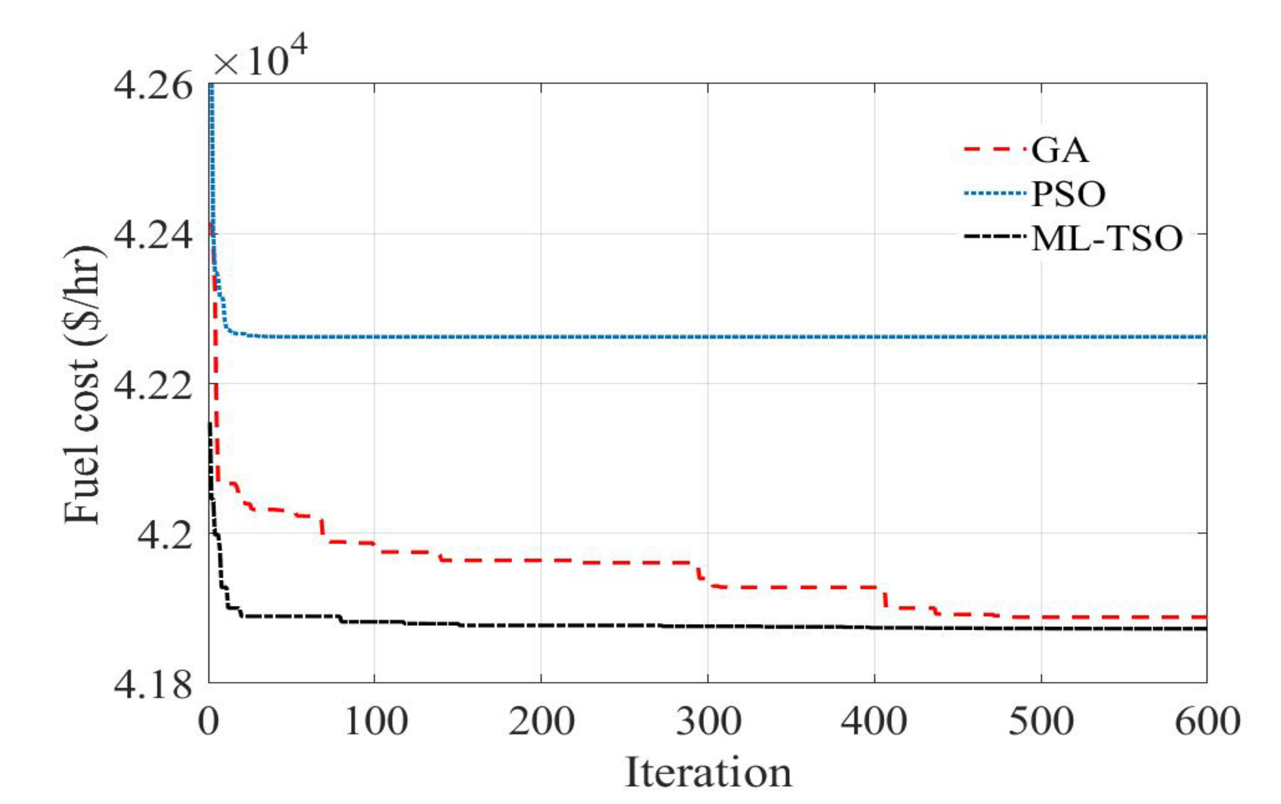
The results obtained by ML-TSO are compared with the solutions achieved by other single optimization algorithms such as GA and PSO. The stopping criterion for the runs of all algorithms is the number of iterations, which is set to 600. The comparisons shown in Table 5 and Table 6 depict the values of the design variables, which are the output power needed from each conventional generating unit in each system to meet the demand of the network. Additionally, the fuel cost in each system needed to operate the generators can be seen. Furthermore, Figure 6 and Figure 7 show the convergence performance of the proposed hybrid algorithm in comparison to other methods while solving the PPF problem; clearly, the optimal results obtained by the proposed hybrid ML-TSO in both applied cases can be seen.

Table 5.
Minimum fuel cost and optimal design variables for the IEEE 57-bus system.

Table 6.
Minimum fuel cost and optimal design variables for the IEEE 118-bus system.
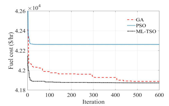
Figure 6.
Cost function vs. iterations in the 57-bus system.
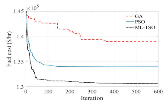
Figure 7.
Cost function vs. iterations in the 118-bus system.
In the case of the IEE 57-bus system, the PSO reached the worst result after 600 iterations. The GA and the proposed ML-TSO methods reached close results, but the proposed ML-TSO method’s result is better. The ML-TSO reached better results than the GA by 0.0441% and better results than the PSO by 0.93%. It can be argued that the ML-TSO convergence performance is better, as it needed about 100 iterations to settle. Meanwhile, the GA needed about 450 iterations.
With respect to the IEEE 118-bus system, the GA reached the worst result after 600 iterations. The proposed ML-TSO method reached the best result. The ML-TSO result is better than that of the GA by 6.4% and better than that of the PSO by 2.56%. Hence, the ML-TSO convergence performance is better, as it needed about 300 iterations to settle. In general, the convergence of the cost function curves in the two standard systems using the ML-TSO method is fast and smooth.
5.2. Probabilistic OPF with RESs Uncertainties and Time-Varying Loads
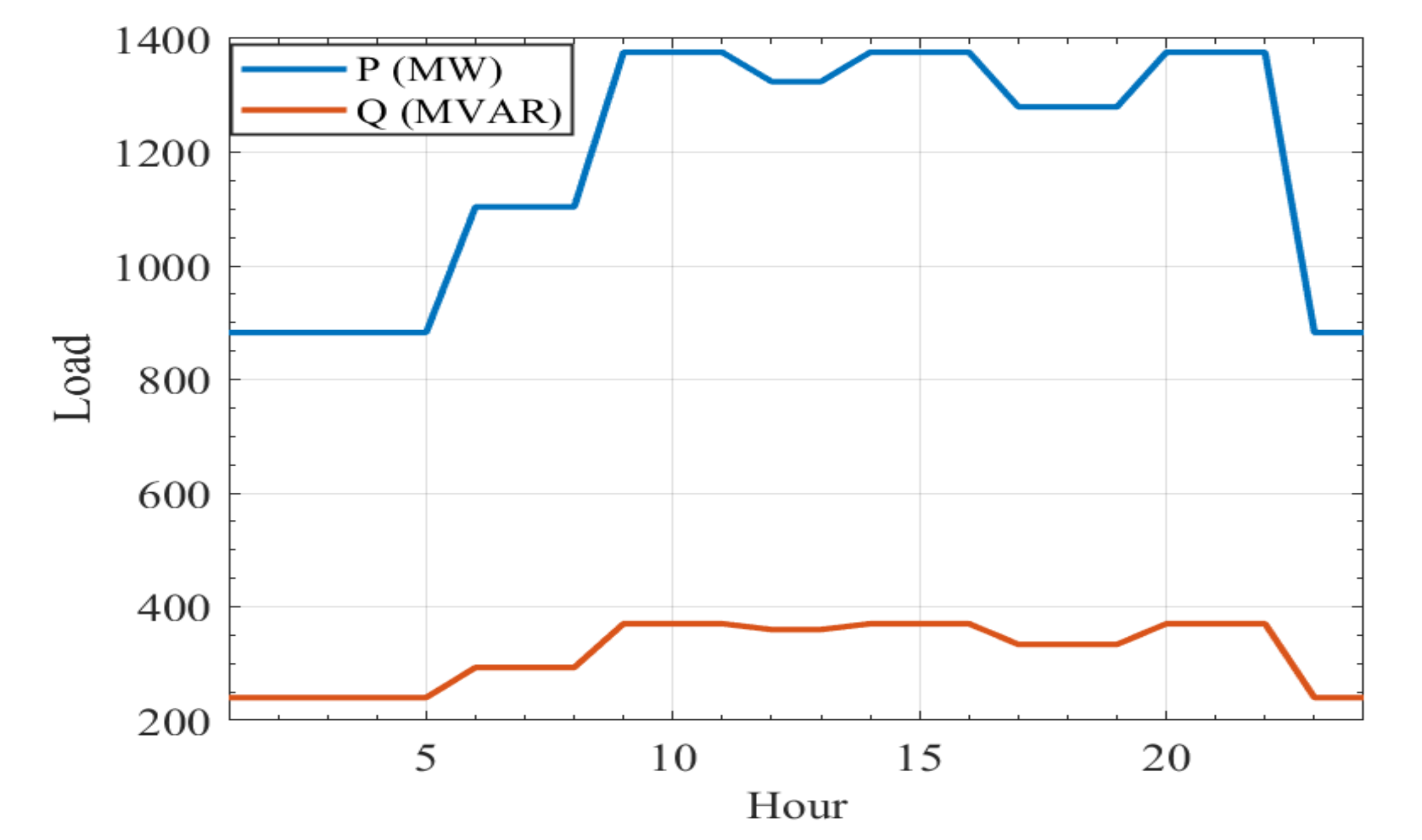
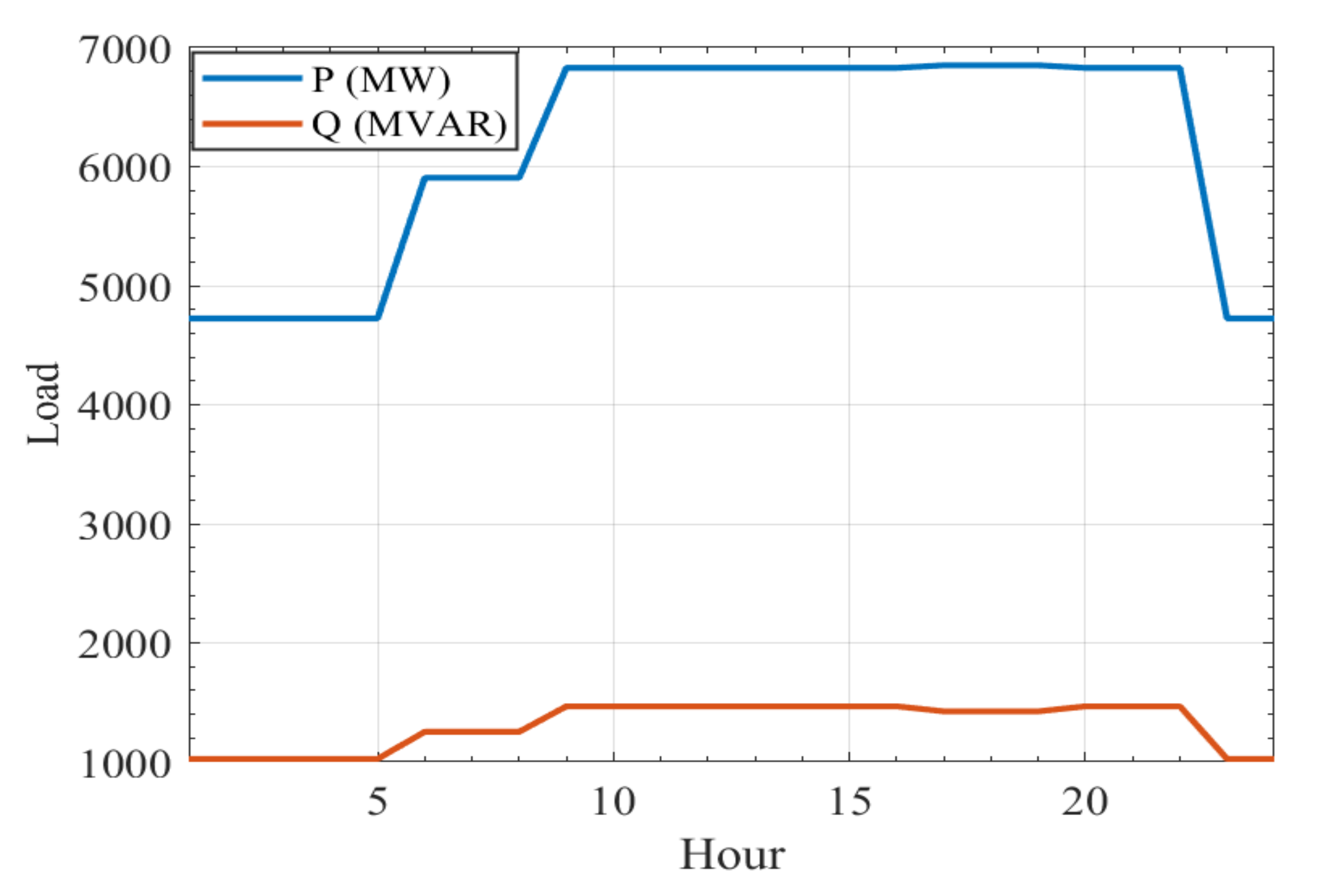
The proposed hybrid ML-TSO algorithm has been applied to solve POPF for the modified IEEE 57- and 118 bus test systems. The RESs (PV and/or WT) are integrated on certain buses in the two test systems, as given in Table 7. Meanwhile, the hourly load demand variation using typical day forecasting is taken into account. The hourly active and reactive power demand variations are given in Figure 8 and Figure 9 for the 57- and 118-bus systems, respectively.

Table 7.
Locations of the RESs in the 57- and the 118-bus systems.
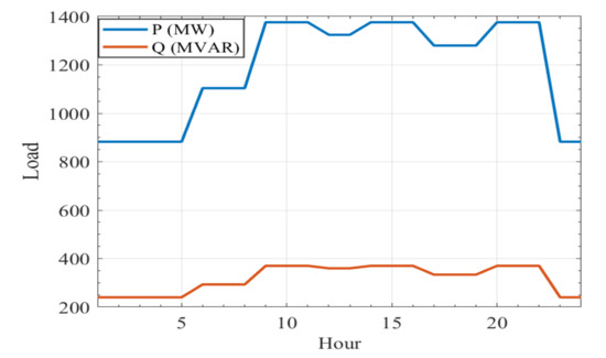
Figure 8.
Hourly demand of the 57-bus system.
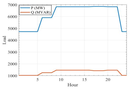
Figure 9.
Hourly demand of the 118-bus system.
The active output power of the PV and WT generators varies through the day according to the irradiance and the wind speed profiles [53,54]. So, in this study, the uncertainties of renewable energy resources [55] are considered when forecasting the hourly active output power of the solar and wind systems. Different cases of POPF are evaluated in this scenario. In the first case, the OPF solution has only been evaluated with the hourly variable load consideration and with no RESs integrated. In second and third cases, the OPF solution is performed with the integration of either PV or WT. Finally, the proposed hybrid ML-TSO was implemented for the POPF solution, including both the PV and WT to the studied test systems.
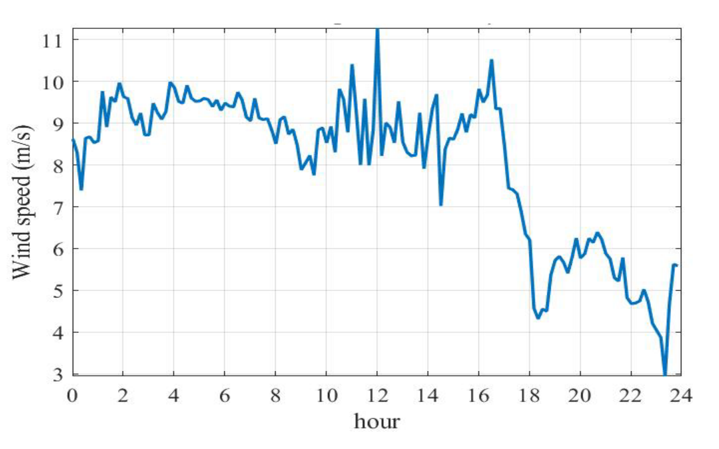
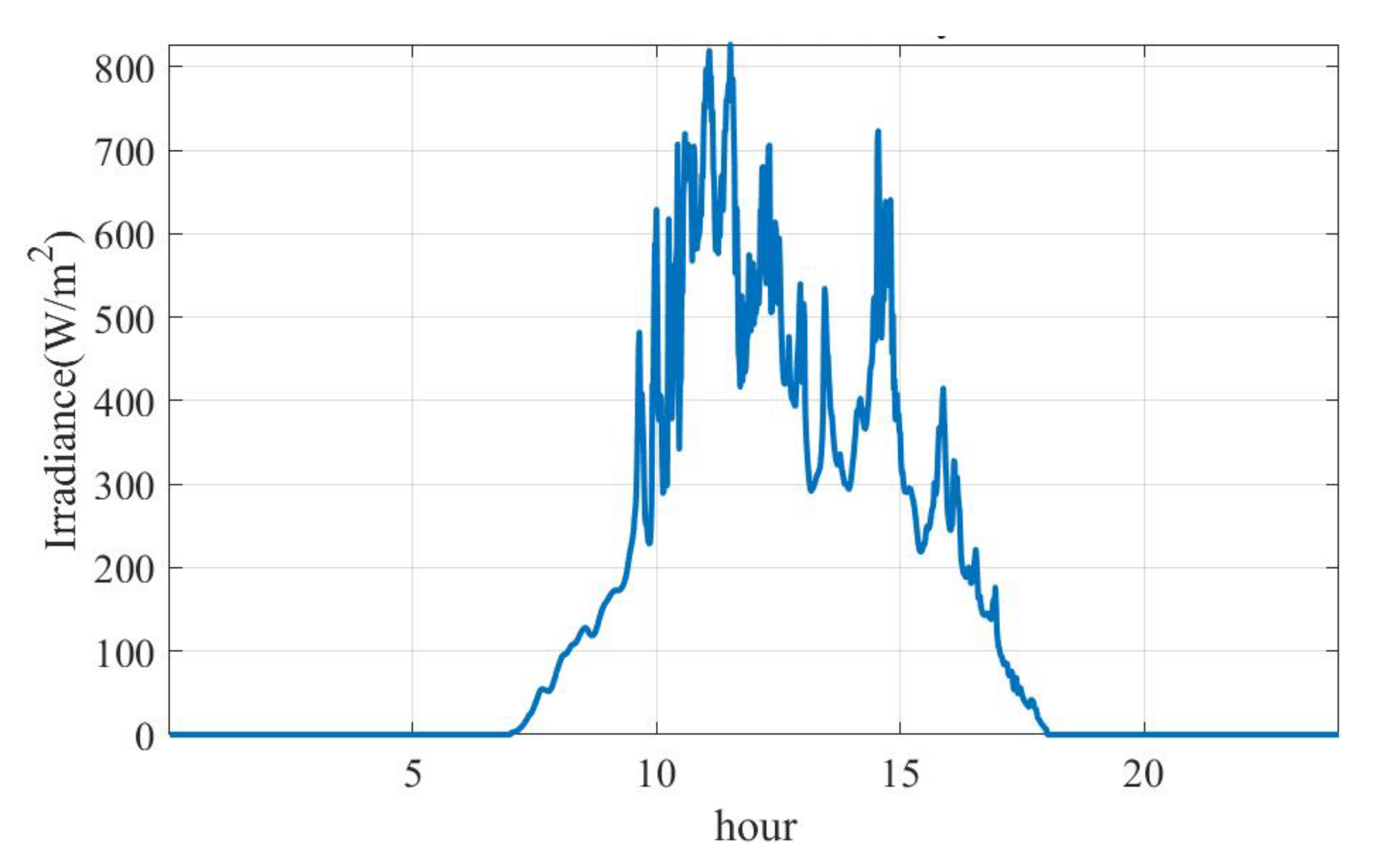
The nominal, cut-in, and cutoff wind speeds are assumed to be 10 m/s, 2.7 m/s, and 25 m/s. The generated active power from the PV system is calculated using (15). At the standard condition of irradiance (Sstc), the solar irradiance is assumed to be 1000 W/m2. Additionally, the certain irradiance point (Rc) is assumed to be 120 W/m2. This part of the research investigates the uncertainty of the RESs and the effect of their variable active power generation on the power generation of the conventional generators, which reflects on the total fuel cost, correspondingly. In this study, it is assumed that renewable energy sources were already installed when defining the cost function. The POPF is performed sequentially through a whole day divided into preset time intervals of 1 h each. The wind speed data were taken in Zafarana in Egypt on 25 November 2014. The solar irradiance data have been obtained from the Natural Energy Laboratory of Hawaii Authority (NELHA) on 3 January 2022. Figure 10 and Figure 11 show the variation of the wind speeds and the solar irradiance throughout a day.
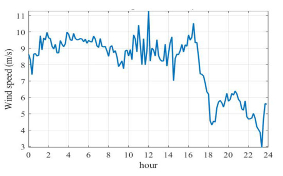
Figure 10.
Measured wind speed throughout the day.

Figure 11.
Measured sun irradiance throughout the day.
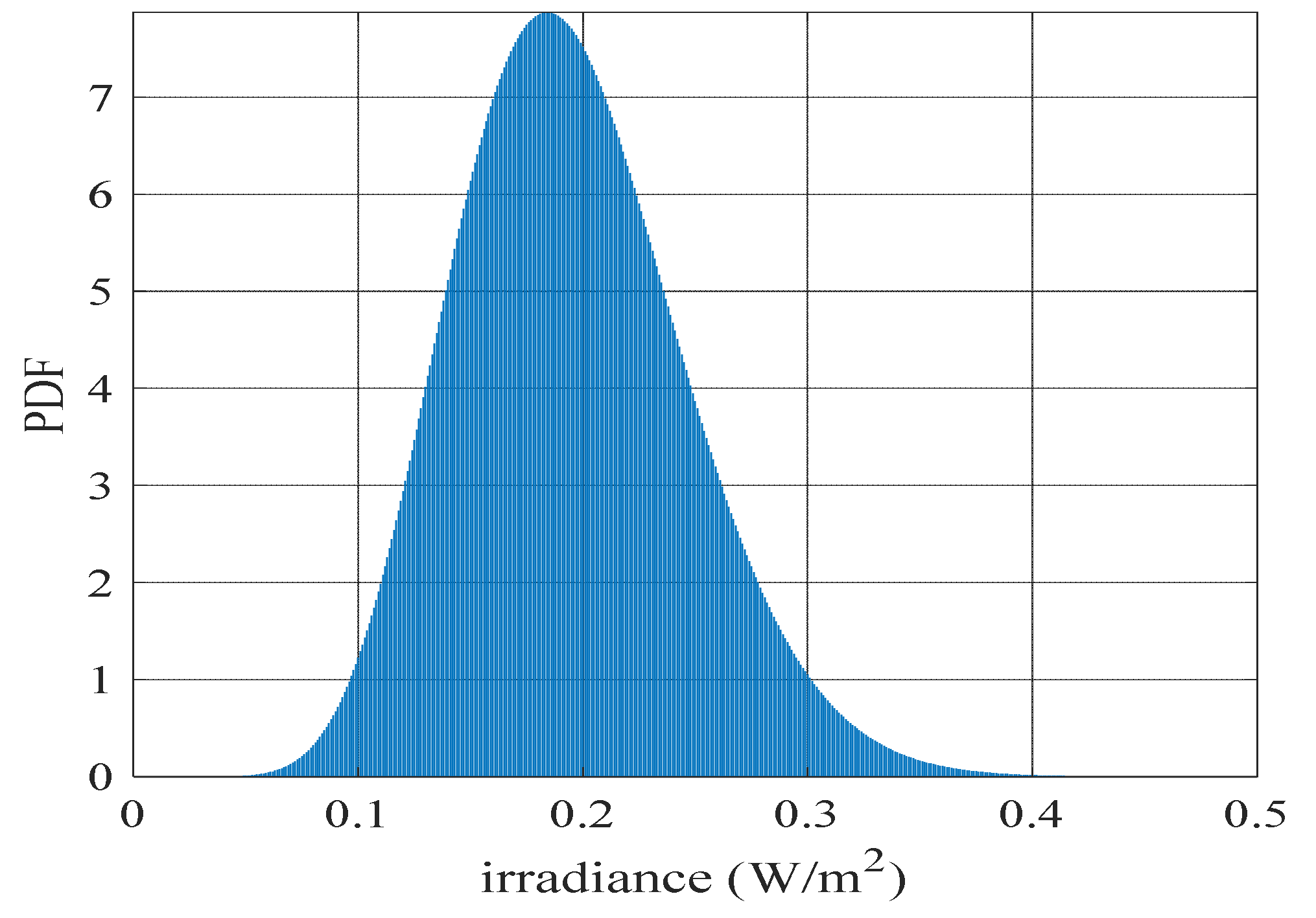
According to the measured data, the PDFs of the wind speeds and the solar irradiance are determined, and a sample of these PDFs, at hour 17, is illustrated in Figure 12 and Figure 13. The forecasted generated active powers from the wind turbine and the PV panel are then calculated using Equations (15) and (19).

Figure 12.
PDF of solar irradiance at hour 17.

Figure 13.
PDF of wind speed at hour 17.
Implementing the proposed methodology on the IEEE 57 bus system, the obtained results in Figure 14 show the hourly cost of four investigated scenarios. The investigated scenarios include the system without RES, the system with only PV or WT energy sources, and both types of RESs integration. It is noted that a reduced cost was obtained when the PV panel was contributing between hours 9 and 18, as it is the duration when the solar irradiance is beneficial to generating maximum power. In contrast, the effect of the wind turbine in the system can be noticed during the entire time slot. However, the maximum cost reduction is recorded between hours 10 and 17. Similarly, the comparison of hourly costs for the four scenarios in the case of the 118-bus system is shown in Figure 15. It can be seen that the proposed hybrid ML-TSO method provides the best optimal solutions for the PPF problem, and the illustrated results show the impact of renewable energy integration subject to fuel cost reduction.
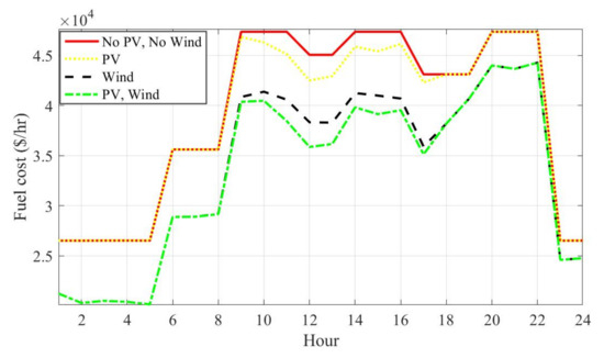
Figure 14.
Hourly fuel cost in the case of the 57-bus system.
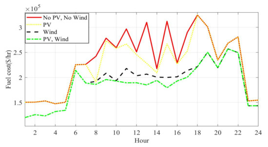
Figure 15.
Hourly fuel cost in the case of the 118-bus system.
5.3. Statistical Analysis of the Classical OPF Results
In order to examine and verify the performance of the proposed hybrid ML-TSO optimization approach, the simulations are repeated for the three optimization methods (ML-TSO, PSO, and GA) using the investigated test system, i.e., the IEEE 57- and 118-bus systems. The performed statistical analysis shows valuable insights regarding the best value, worst value, mean value, median value, and standard deviation.
Table 8 and Table 9 show the statistical indicators for the two investigated test systems, where the statistic obtained by the proposed ML-TSO method outperforms the other techniques. For instance, using the optimization parameters, the standard deviation calculated by the ML-TSO method is the lowest in both investigated systems. The obtained results prove the consistency, relevance and robustness of the proposed optimization method.

Table 8.
The best, worst, mean, median, and standard deviation values in the case of the 57-bus system.

Table 9.
The best, worst, mean, median, and standard deviation values in the case of the 118-bus system.
The meta-heuristic techniques are known for their uncertainty in results over the repetition of the runs of the simulation. One of the tests used to verify how robust the metaheuristic algorithm is is Wilcoxon’s rank-sum test. This test provides a fair comparison among the introduced ML-TSO method and the PSO and GA optimization methods. Twenty independent runs are implemented in the test. The selected level of significance is 5%. The p-values determined by Wilcoxon’s rank-sum test are shown in Table 10. The h-values obtained from the test is ‘1′, which means that the null hypothesis is rejected among the optimization algorithms. It can be concluded from the test results that the ML-TSO is superior to the PSO and the GA optimization methods when applied to solve the OPF and PPF problems under the different scenarios stated previously in the problem formulation.

Table 10.
p-Values of Wilcoxon’s rank-sum test.
6. Conclusions
This paper has introduced a novel hybrid optimization method based on the combination of TSO and machine learning techniques, namely, a hybrid ML-TSO algorithm with the main target of solving the classic OPF and POPF problems optimally. The main inferences of the paper can be given in bullets as follows:
- The proposed hybrid ML-TSO algorithm’s implementation of the solution of the OPF and PPF problems was verified on standard IEEE 57-bus and 118-bus systems.
- The results and statistics demonstrate the applicability of the hybrid ML-TSO algorithm, as the convergence performance was observed to be better than that of the other optimization algorithms.
- The application of the ML-TSO for the OPF resulted in a reduction in the fuel costs of 0.0441% to 0.93% for the IEEE 57-bus system.
- The application of the ML-TSO for the OPF resulted in a reduction in the fuel costs of 2.56% to 6.4% for the IEEE 118-bus system.
- The ML-TSO effectively solves the PPF by using distribution functions to simulate the stochastic nature of solar irradiance and wind speed over an entire day.
In the PPF solution strategy, different cases were investigated and analyzed based on the penetration level of the RESs, in which the implications of each case for the calculations were analyzed and evaluated in detail. The findings show that the fuel cost has been significantly minimized when the solar and wind turbine generators were simultaneously added to either the IEEE-57 or 118-bus systems in comparison with a single integration of each source. Lately, the statistical analysis confirms the superior performance of the proposed ML-TSO over that of the PSO and GA algorithms. Finally, it is recommended to use the hybrid ML-TSO optimization method to solve further optimization problems in the field of renewable energy systems and smart grids.
Author Contributions
H.M.H.: Formal analysis, investigation of the results and the proposed algorithm, methodology suggestion, supervision, validation of the results, review and editing of the article; S.F.M.; M.H.Q.; Z.U.; M.T.-V.; R.A.T.; F.J.; M.R.E.; M.A.M.S.; S.A.: Software modification, simulation, writing, and editing. All authors have read and agreed to the published version of the manuscript.
Funding
This work was supported by the Researchers Supporting Project number (RSP-2021/307), King Saud University, Riyadh, Saudi Arabia.
Institutional Review Board Statement
Not applicable.
Informed Consent Statement
Not applicable.
Data Availability Statement
Not applicable.
Acknowledgments
This work was supported by the Researchers Supporting Project number (RSP-2021/307), King Saud University, Riyadh, Saudi Arabia.
Conflicts of Interest
The authors declare no conflict of interest.
References
- Abdi, H.; Beigvand, S.D.; Scala, M.L. A review of optimal power flow studies applied to smart grids and microgrids. Renew. Sustain. Energy Rev. 2017, 71, 742–766. [Google Scholar] [CrossRef]
- Naderi, E.; Pourakbari-Kasmaei, M.; Cerna, F.V.; Lehtonen, M. A novel hybrid self-adaptive heuristic algorithm to handle single- and multi-objective optimal power flow problems. Int. J. Electr. Power Energy Syst. 2021, 125, 106492. [Google Scholar] [CrossRef]
- de Mel, I.; Klymenko, O.V.; Short, M. Balancing accuracy and complexity in optimisation models of distributed energy systems and microgrids with optimal power flow: A review. Sustain. Energy Technol. Assess. 2022, 52, 102066. [Google Scholar] [CrossRef]
- Kahraman, H.T.; Akbel, M.; Duman, S. Optimization of Optimal Power Flow Problem Using Multi-Objective Manta Ray Foraging Optimizer. Appl. Soft Comput. 2022, 116, 108334. [Google Scholar] [CrossRef]
- Naderi, E.; Pourakbari-Kasmaei, M.; Abdi, H. An efficient particle swarm optimization algorithm to solve optimal power flow problem integrated with FACTS devices. Appl. Soft Comput. 2019, 80, 243–262. [Google Scholar] [CrossRef]
- Nguyen, T.T. A high performance social spider optimization algorithm for optimal power flow solution with single objective optimization. Energy 2019, 171, 218–240. [Google Scholar] [CrossRef]
- Giraldo, J.S.; Lopez, J.C.; Castrillon, J.A.; Rider, M.J.; Castro, C.A. Probabilistic OPF Model for Unbalanced Three-Phase Electrical Distribution Systems Considering Robust Constraints. IEEE Trans. Power Syst. 2019, 34, 3443–3454. [Google Scholar] [CrossRef]
- Capitanescu, F. Critical review of recent advances and further developments needed in AC optimal power flow. Electr. Power Syst. Res. 2016, 136, 57–68. [Google Scholar] [CrossRef]
- Elattar, E.E. Optimal Power Flow of a Power System Incorporating Stochastic Wind Power Based on Modified Moth Swarm Algorithm. IEEE Access 2019, 7, 89581–89593. [Google Scholar] [CrossRef]
- Khan, I.U.; Javaid, N.; Gamage, K.A.A.; Taylor, C.J.; Baig, S.; Ma, X. Heuristic Algorithm Based Optimal Power Flow Model Incorporating Stochastic Renewable Energy Sources. IEEE Access 2020, 8, 148622–148643. [Google Scholar] [CrossRef]
- Elattar, E.E.; ElSayed, S.K. Modified JAYA algorithm for optimal power flow incorporating renewable energy sources considering the cost, emission, power loss and voltage profile improvement. Energy 2019, 178, 598–609. [Google Scholar] [CrossRef]
- Meng, A.; Zeng, C.; Wang, P.; Chen, D.; Zhou, T.; Zheng, X.; Yin, H. A high-performance crisscross search based grey wolf optimizer for solving optimal power flow problem. Energy 2021, 225, 120211. [Google Scholar] [CrossRef]
- Zhou, S.; Xiao, Q.; Wu, L. Probabilistic power flow analysis with correlated wind speeds. Renew. Energy 2020, 145, 2169–2177. [Google Scholar] [CrossRef]
- Khan, B.S.; Raja, M.A.Z.; Qamar, A.; Chaudhary, N.I. Design of moth flame optimization heuristics for integrated power plant system containing stochastic wind. Appl. Soft Comput. 2021, 104, 107193. [Google Scholar] [CrossRef]
- Ramadhani, U.H.; Shepero, M.; Munkhammar, J.; Widén, J.; Etherden, N. Review of probabilistic load flow approaches for power distribution systems with photovoltaic generation and electric vehicle charging. Int. J. Electr. Power Energy Syst. 2020, 120, 106003. [Google Scholar] [CrossRef]
- Prusty, B.R.; Jena, D. A critical review on probabilistic load flow studies in uncertainty constrained power systems with photovoltaic generation and a new approach. Renew. Sustain. Energy Rev. 2017, 69, 1286–1302. [Google Scholar] [CrossRef]
- Ullah, Z.; Wang, S.; Wu, G.; Hasanien, H.M.; Jabbar, M.W.; Qazi, H.S.; Tostado-Véliz, M.; Turky, R.A.; Elkadeem, M.R. Advanced studies for probabilistic optimal power flow in active distribution networks: A scientometric review. IET Gener. Transm. Distrib. 2022, 16, 3579–3604. [Google Scholar] [CrossRef]
- Papadimitrakis, M.; Giamarelos, N.; Stogiannos, M.; Zois, E.N.; Livanos, N.A.I.; Alexandridis, A. Metaheuristic search in smart grid: A review with emphasis on planning, scheduling and power flow optimization applications. Renew. Sustain. Energy Rev. 2021, 145, 111072. [Google Scholar] [CrossRef]
- Skolfield, J.K.; Escobedo, A.R. Operations research in optimal power flow: A guide to recent and emerging methodologies and applications. Eur. J. Oper. Res. 2022, 300, 387–404. [Google Scholar] [CrossRef]
- González-Ordiano, J.Á.; Mühlpfordt, T.; Braun, E.; Liu, J.; Çakmak, H.; Kühnapfel, U.; Düpmeier, C.; Waczowicz, S.; Faulwasser, T.; Mikut, R.; et al. Probabilistic forecasts of the distribution grid state using data-driven forecasts and probabilistic power flow. Appl. Energy 2021, 302, 117498. [Google Scholar] [CrossRef]
- Gallego, L.A.; Franco, J.F.; Cordero, L.G. A fast-specialized point estimate method for the probabilistic optimal power flow in distribution systems with renewable distributed generation. Int. J. Electr. Power Energy Syst. 2021, 131, 107049. [Google Scholar] [CrossRef]
- Wang, C.; Liu, D.; Tang, F.; Liu, C. A clustering-based analytical method for hybrid probabilistic and interval power flow. Int. J. Electr. Power Energy Syst. 2021, 126, 106605. [Google Scholar] [CrossRef]
- Su, C.; Liu, C.; Jiang, S.; Wang, Y. Probabilistic power flow for multiple wind farms based on RVM and holomorphic embedding method. Int. J. Electr. Power Energy Syst. 2021, 130, 106843. [Google Scholar] [CrossRef]
- Huang, Y.; Chen, S.; Chen, Z.; Huang, Q.; Hu, W. Probabilistic load flow computation considering dependence of wind powers and using quasi-Monte Carlo method with truncated regular vine copula. Int. Trans. Electr. Energy Syst. 2020, 30, e12646. [Google Scholar] [CrossRef]
- Duman, S.; Rivera, S.; Li, J.; Wu, L. Optimal power flow of power systems with controllable wind-photovoltaic energy systems via differential evolutionary particle swarm optimization. Int. Trans. Electr. Energy Syst. 2020, 30, e12270. [Google Scholar] [CrossRef]
- Sulaiman, M.H.; Mustaffa, Z.; Mohamad, A.J.; Saari, M.M.; Mohamed, M.R. Optimal power flow with stochastic solar power using barnacles mating optimizer. Int. Trans. Electr. Energy Syst. 2021, 31, e12858. [Google Scholar] [CrossRef]
- Sulaiman, M.H.; Mustaffa, Z. Solving optimal power flow problem with stochastic wind–solar–small hydro power using barnacles mating optimizer. Control Eng. Pract. 2021, 106, 104672. [Google Scholar] [CrossRef]
- Shilaja, C.; Arunprasath, T. Optimal power flow using Moth Swarm Algorithm with Gravitational Search Algorithm considering wind power. Futur. Gener. Comput. Syst. 2019, 98, 708–715. [Google Scholar]
- Guvenc, U.; Duman, S.; Kahraman, H.T.; Aras, S.; Katı, M. Fitness–Distance Balance based adaptive guided differential evolution algorithm for security-constrained optimal power flow problem incorporating renewable energy sources. Appl. Soft Comput. 2021, 108, 107421. [Google Scholar] [CrossRef]
- Ullah, Z.; Wang, S.; Radosavljevic, J.; Lai, J. A Solution to the Optimal Power Flow Problem Considering WT and PV Generation. IEEE Access 2019, 7, 46763–46772. [Google Scholar] [CrossRef]
- Shaheen, M.A.M.; Hasanien, H.M.; Al-Durra, A. Solving of optimal power flow problem including renewable energy resources using HEAP optimization algorithm. IEEE Access 2021, 9, 35846–35863. [Google Scholar] [CrossRef]
- Samakpong, T.; Ongsakul, W.; Madhu Manjiparambil, N. Optimal power flow incorporating renewable uncertainty related opportunity costs. Comput. Intell. 2020, 38, 1057–1082. [Google Scholar] [CrossRef]
- Jithendranath, J.; Das, D.; Guerrero, J.M. Probabilistic optimal power flow in islanded microgrids with load, wind and solar uncertainties including intermittent generation spatial correlation. Energy 2021, 222, 119847. [Google Scholar] [CrossRef]
- Ye, K.; Zhao, J.; Zhang, Y.; Liu, X.; Zhang, H. A generalized computationally efficient copula-polynomial chaos framework for probabilistic power flow considering nonlinear correlations of PV injections. Int. J. Electr. Power Energy Syst. 2022, 136, 107727. [Google Scholar] [CrossRef]
- Peng, S.; Lin, X.; Tang, J.; Xie, K.; Ponci, F.; Monti, A.; Li, W. Probabilistic Power Flow of AC/DC Hybrid Grids with Addressing Boundary Issue of Correlated Uncertainty Sources. IEEE Trans. Sustain. Energy 2022, 13, 1607–1619. [Google Scholar] [CrossRef]
- Xiao, Q.; Wu, L.; Chen, C. Probabilistic power flow computation using nested point estimate method. IET Gener. Transm. Distrib. 2022, 16, 1064–1082. [Google Scholar] [CrossRef]
- Kurt, U.; Ozgonenel, O.; Ayvaz, B.B. Probabilistic Power Flow Analysis Using Matlab Graphical User Interface (GUI). J. Electr. Eng. Technol. 2022, 17, 929–943. [Google Scholar] [CrossRef]
- Ağbulut, Ü.; Gürel, A.E.; Biçen, Y. Prediction of daily global solar radiation using different machine learning algorithms: Evaluation and comparison. Renew. Sustain. Energy Rev. 2021, 135, 110114. [Google Scholar] [CrossRef]
- Dastile, X.; Celik, T.; Potsane, M. Statistical and machine learning models in credit scoring: A systematic literature survey. Appl. Soft Comput. 2020, 91, 106263. [Google Scholar] [CrossRef]
- Qais, M.H.; Hasanien, H.M.; Alghuwainem, S. Transient search optimization for electrical parameters estimation of photovoltaic module based on datasheet values. Energy Convers. Manag. 2020, 214, 112904. [Google Scholar] [CrossRef]
- Shaheen, M.A.M.; Hasanien, H.M.; Mekhamer, S.F.; Talaat, H.E.A. Optimal power flow of power systems including distributed generation units using sunflower optimization algorithm. IEEE Access 2019, 7, 109289–109300. [Google Scholar] [CrossRef]
- Yang, Y.; Yang, Z.; Yu, J.; Zhang, B.; Zhang, Y.; Yu, H. Fast Calculation of Probabilistic Power Flow: A Model-Based Deep Learning Approach. IEEE Trans. Smart Grid 2020, 11, 2235–2244. [Google Scholar] [CrossRef]
- Wang, H.; Yan, Z.; Xu, X.; He, K. Probabilistic power flow analysis of microgrid with renewable energy. Int. J. Electr. Power Energy Syst. 2020, 114, 105393. [Google Scholar] [CrossRef]
- Reddy, Y.; Jithendranath, J.; Chakraborty, A.K.; Guerrero, J.M. Stochastic optimal power flow in islanded DC microgrids with correlated load and solar PV uncertainties. Appl. Energy 2022, 307, 118090. [Google Scholar]
- Jiang, P.; Liu, Z.; Niu, X.; Zhang, L. A combined forecasting system based on statistical method, artificial neural networks, and deep learning methods for short-term wind speed forecasting. Energy 2021, 217, 119361. [Google Scholar] [CrossRef]
- Hasanien, H.M.; Shaheen, M.A.M.; Turky, R.A.; Qais, M.H.; Alghuwainem, S.; Kamel, S.; Tostado-Véliz, M.; Jurado, F. Precise modeling of PEM fuel cell using a novel Enhanced Transient Search Optimization algorithm. Energy 2022, 247, 123530. [Google Scholar] [CrossRef]
- Qais, M.H.; Hasanien, H.M.; Alghuwainem, S. Transient search optimization: A new meta-heuristic optimization algorithm. Appl. Intell. 2020, 50, 3926–3941. [Google Scholar] [CrossRef]
- Chegini, S.N.; Bagheri, A.; Najafi, F. PSOSCALF: A new hybrid PSO based on Sine Cosine Algorithm and Levy flight for solving optimization problems. Appl. Soft Comput. 2018, 73, 697–726. [Google Scholar] [CrossRef]
- Khalid Saeed, M.; Salam, A.; Rehman, A.U.; Abid Saeed, M. Comparison of six different methods of Weibull distribution for wind power assessment: A case study for a site in the Northern region of Pakistan. Sustain. Energy Technol. Assess. 2019, 36, 100541. [Google Scholar] [CrossRef]
- Cuevas, E.; Galvez, J. An optimization algorithm guided by a machine learning approach. Int. J. Mach. Learn. Cybern. 2019, 10, 2963–2991. [Google Scholar] [CrossRef]
- Wickramasinghe, C.S.; Amarasinghe, K.; Manic, M. Deep Self-Organizing Maps for Unsupervised Image Classification. IEEE Trans. Ind. Inform. 2019, 15, 5837–5845. [Google Scholar] [CrossRef]
- Qu, X.; Yang, L.; Guo, K.; Ma, L.; Sun, M.; Ke, M.; Li, M. A Survey on the Development of Self-Organizing Maps for Unsupervised Intrusion Detection. Mob. Netw. Appl. 2021, 26, 808–829. [Google Scholar] [CrossRef]
- Li, S.; Gong, W.; Wang, L.; Gu, Q. Multi-objective optimal power flow with stochastic wind and solar power. Appl. Soft Comput. 2022, 114, 108045. [Google Scholar] [CrossRef]
- Javad Aliabadi, M.; Radmehr, M. Optimization of hybrid renewable energy system in radial distribution networks considering uncertainty using meta-heuristic crow search algorithm. Appl. Soft Comput. 2021, 107, 107384. [Google Scholar] [CrossRef]
- Kaymaz, E.; Duman, S.; Guvenc, U. Optimal power flow solution with stochastic wind power using the Lévy coyote optimization algorithm. Neural Comput. Appl. 2021, 33, 6775–6804. [Google Scholar] [CrossRef]
Publisher’s Note: MDPI stays neutral with regard to jurisdictional claims in published maps and institutional affiliations. |
© 2022 by the authors. Licensee MDPI, Basel, Switzerland. This article is an open access article distributed under the terms and conditions of the Creative Commons Attribution (CC BY) license (https://creativecommons.org/licenses/by/4.0/).

