What Drives Economic Growth across European Countries? A Multimodal Approach

Abstract

This research study examines the factors that determined economic growth measured by gross domestic product, gross value added, final consumption expenditure of households, and gross fixed capital formation across a sample of 36 European countries during the time frame Q3 2018−Q3 2021. We conducted a panel data analysis with the first-difference generalized method of moments (GMM) approach and cross-section fixed effects. Empirical results estimated with four econometric models indicated a significant robust impact of the independent variables exports, imports, foreign direct investment inflow, foreign direct investment outflow, social contributions, and wages on economic growth proxies. In addition, multiplex network analysis was used to investigate the connection architectures of the 36 countries, and it yielded statistical measurements for all layers in the multi-layered structure. Relevant policy implications of reported empirical results are also addressed.

1. Introduction

The phenomenon of economic growth and its factors of influence have been a long-standing topic of interest in the mainstream literature. The reason is straightforward: economic growth captures the capacity of a national economy to augment across time the nominal or inflation-adjusted value of its goods and services, namely its wealth [1,2,3]. A growing economy is usually associated with an increasing interest on behalf of foreign investors, rising income levels, job creation, and improved living standards [4,5,6,7].

Competitiveness level within an economy is commonly associated with economic performance measured by economic growth [8]. Hence, one of the main policy goals for any country should be to stimulate economic output as a necessary base for economic and social development [9,10].

The phenomenon of economic growth is generally measured with the growth rate of the gross domestic product (GDP) [11,12,13,14,15]. With respect to economic growth, we believe that the performance of a national economy can also be measured with other indicators, such as gross value added (GVAD), final consumption expenditure of households (FCEH), and gross fixed capital formation (GFCF).

The main objective of our study was to analyze the determinants of economic growth across European countries during a four-year time span. The phenomenon of economic growth was investigated under the impact of relevant macroeconomic indicators (exports, imports, various types of investments, wages, and social contributions) retrieved from the Eurostat database. The study sample included 36 European countries (see Appendix A), and the period of analysis spanned the quarters Q3 2018−Q3 2021.

Sometimes, standard economic theory limits the study of economic activity to studying the behavior of individual people. Over time, agents in macroeconomic markets learn to alter their interactions, decreasing ineffective ones and strengthening advantageous ones. The patterns of their shared history and economic interaction represent the basis of economies worldwide. The freedom of individual agents to operate and reason must be restrained by setting criteria based on which price judgments must be made. In this context, macroeconomic markets may be regarded as a network in which agents exert influence on one another via a variety of interactions with other nodes [16,17,18,19].

A firm, an individual, or an economic area may be regarded as network nodes that represent interacting actors. Numerous connections between nodes are represented in networks, which are effective interdisciplinary modeling tools. Consequently, a network is an essential tool in modern times for understanding the linked world, which includes financial and economic aspects [20,21]. Using a number of global network models, the structure of a network with several nodes and/or connections may be better comprehended. In contrast to standard micro- and macro-economic models, network models take into consideration an entire system. Consequently, they provide the dynamics of links and nodes. Identifying pertinent system nodes may be required to design successful policy responses. In this increasingly interconnected world, network analysis may be useful for mapping the economic behavior of countries and assessing the power density of nodes in crucial sectors. In addition, it may be used to: describe the length and distribution of value chains; examine changes caused by the realignment of certain economic activities; investigate the extent to which critical technologies depend on inputs.

Due to multiple contexts in which network-based methodologies may be used, and due to the insights that this modeling technique may provide, network science is deemed as very important for policymaking in economic contexts. Socioeconomic systems are complex and interconnected, a reality that policymakers and regulators must address. Hence, the ability to map and analyze the complex network of technical, economic, and social connections is crucial in formulating and implementing rational policies [22,23,24,25,26,27].

Similarities or differences between the time series of key variables may be used to develop network architectures that simulate interaction or cooperation across countries in various economic contexts. Using distance functions computed on time series, a graph may be utilized combinatorically to create a weighted topology of a network. However, a single variable is inadequate to define countries that connect or collaborate. In this study, in addition to panel data models, multiplex multilayer network topologies are applied to depict such multivariate interactions.

In terms of mathematical contributions, the novelty of this study resides in that we investigate the dynamics of the relationships between countries with multiplex network analysis. In recent decades, times series analysis received input from various disciplines such as nonlinear dynamics, statistical physics, computer science, and Bayesian statistics, resulting in new approaches such as nonlinear time series analysis or data mining [28,29]. More recently, the science of complex networks has aided in the development of a novel approach to time series analysis based on the transformation of a time series into a network according to a specified mapping algorithm, followed by the extraction of the time series information by analyzing the derived network [30]. Within this framework, a traditional possibility is to interpret the interdependencies between time series (encapsulated, for example, in cross-correlation matrices) as weighted edges of a graph. The graph nodes label each time series, yielding functional networks that have been used fruitfully and extensively in fields such as neuroscience and finance [31,32].

The methodological approach is complex and includes descriptive statistics, correlation analysis, and econometric estimations by means of panel first-difference generalized method of moments (GMM) with cross-section effects and multiplex network analysis. Empirical results revealed that the chosen macroeconomic indicators played a fundamental role for the economic growth of our sample of European countries. More specifically, the levels of economic growth were boosted as national imports, exports, and social contributions increased. In addition, the multiplex network analysis elicited connection architectures (i.e., cooperation and interaction) of the 36 nations considered, and produced statistical metrics of every layer in the multi-layered multiplex structure.

The remainder of the paper has the following structure. Section 2 surveys relevant studies on determinants of economic growth. Section 3 presents the variables, research hypotheses, econometric models, and empirical results. Section 4 reports on the multiplex network analysis and related outcomes. Section 5 details briefly on the main results, policy implications, and upcoming research directions.

2. Literature Review

The following section delves into relevant research examining the factors that drive economic growth worldwide. The fundamental role of this literature survey stems from the fact that it served to identify certain independent variables and formulate research hypotheses starting from these studies.

The literature on economic growth has reported multiple studies on the factors that influence it to a great extent. In this sense, Pegkas, Staikouras, and Tsamadias [33] investigated the economic growth phenomenon in the Eurozone across several years and found that economic growth levels improved after an increase in investment, human capital, trade openness, and public debt. At the same time, authors reported a mitigation in economic growth as public debt increased, therefore eliciting a mixed connection between economic growth and public debt. Asheghian [34] examined the phenomenon in the United States across 40 years and found a unidirectional relationship between foreign direct investment growth and economic growth. Moreover, this phenomenon was also considerably shaped by total factor productivity growth and domestic investment growth.

The study of Chen and Feng [35] investigated how economic growth varied between 29 provinces, municipalities, and autonomous regions in China. The authors found that economic growth was stimulated by higher education, and private and semi-private enterprises in addition to international trade. Furthermore, factors such as high inflation and the presence of state-owned companies mitigated economic growth across Chinese divisions.

Sokhanvar and Jenkins [36] focused on the Estonian economy and showed that the country’s long-term economic growth was positively influenced by macroeconomic variables, such as international tourism and foreign direct investment inflow. Ciccone and Jarocinski [37] conducted an engaging study on the robustness of economic growth determinants by comparing World Bank income data and Penn World Table income data. Authors concluded that the methodology of computing significant determinants was “sensitive to income differences across datasets”.

Using data from 50 countries on five continents, Batrancea et al. [38] studied the phenomenon during the period 1971−2020 by monitoring the sustainability feature of economic growth. Results indicated that domestic credits granted to the private sector by banks and the financial sector were among the relevant determinants, aside from value added from agriculture, forestry, and fishing, or carbon dioxide and nitrous oxide emissions. In the same vein, a study examining economic growth in 34 African countries [39] across two decades showed that the phenomenon was considerably shaped by imports, exports, gross capital formation, and gross domestic savings.

Vedia-Jerez and Chasco [40] reported empirical results on a sample of South American nations for the period 1960−2008 based on two equations. They found that economic growth was significantly influenced by human and physical capital accumulation, along with sectorial exports.

By employing data from 21 OECD countries during the time span 1971−1998, Bassani and Scarpetta [41] concluded that economic growth was positively influenced by the degree of stock market capitalization. Nevertheless, it was negatively impacted by high inflation and the overall size of the government.

3. Methodology

Table 1. Description of variables with definitions and symbols.

Variables	Symbol	Variable Definition
DEPENDENT VARIABLES
Gross domestic product	GDP	Gross domestic product at current prices (%). It compares the quarterly value of a country’s GDP to the corresponding quarterly GDP value from 2010 in order to determine the economy growth level.
Gross value added	GVAD	Gross value added at current prices (%). It indicates productivity and captures the contributions of corporate subsidiaries, companies, and municipalities to a national economy. It is computed by dividing quarterly GVAD values to the corresponding quarterly GVAD values from 2010.
Final consumption expenditure of households	FCEH	Final consumption expenditure of households at current price (%). It comprises the expenses of resident households with goods and services, which are intended to serve one’s needs or wants. The indicator encompasses only the share of expenses with health, education, and housing, remaining to be paid after potential reimbursements. It is computed by dividing quarterly FCEH values to the corresponding quarterly FCEH values from 2010.
Gross fixed capital formation	GFCF	Gross fixed capital formation atcurrentprices (%). It captures the investments in fixed assets of resident producers, after deducting disposals, during a given period. The category of fixed assets includes tangible or intangible assets that result from production processes. Such assets are used multiple times or continuously for periods over a year. It is computed by dividing quarterly GFCF values to the corresponding quarterly GFCF values from 2010.
INDEPENDENT VARIABLES
Imports	IMP	Imports at current prices as a percent of GDP (%). Imports refer to products or services produced abroad and purchased in a specific country.
Exports	EXP	Exports at current prices as a percent of GDP (%). Exports refer to goods and services that are produced in one country and sold to buyers in another country.
Foreign direct investment inflow	FDII	Foreign direct investment inflow as a percent of GDP (%). Such financial inflows comprise equity transactions, earnings reinvestment, and intercompany debt transactions.
Foreign direct investment outflow	FDIO	Foreign direct investment outflow as a percent of GDP (%). Such investments comprise assets and liabilities transferred between resident direct investors and their direct investment enterprises.
Portfolio investment inflow	PII	Portfolio investment inflow at current prices as a percent of GDP (%). Foreign portfolio investment refers to holding financial assets from a country outside of the investor’s own country.
Portfolio investment outflow	PIO	Portfolio investment outflow at current prices as a percent of GDP (%). Domestic portfolio investment refers to holding financial assets in a country outside of the investor’s own country.
Wages	W	Wages as a percent of GDP (%). Wages are fixed regular payments obtained in exchange of work or services, which is generally paid daily or weekly.
Social contributions	SC	Social contributions as a percent of GDP (%). These are payments to social insurance schemes in order to secure the covering of social insurance benefits provided to taxpayers.

presents all variables of interest used in our study, with corresponding symbols and definitions. Variables were selected based on surveying relevant studies in the literature (see Section 2) in addition to authors’ input. Values for each variable of interest were retrieved from the Eurostat database [42], which provided quarterly observations for the period spanning the third quarter of 2018 until the third quarter of 2021, hence securing a balanced panel dataset that included all countries altogether.

In the following we present the research hypotheses and the general form of the proposed econometric models. We used the statistical software EViews version 10 to estimate econometric models with the panel first-difference generalized method of moments (GMM) and cross-section effects [43]. Our choice for this method was motivated by the multiple benefits it entails in estimating results: (1) control for unobserved country heterogeneity; (2) control for measurement error; (3) control for omitted variable bias; (4) control for endogeneity.

According to the literature, especially the studies conducted by Baltagi [44], we applied the Hausman test in order to choose between fixed effects and random effects models. In case the p-value is significant, the literature recommends choosing fixed effects models. Contrariwise, random effects models should be estimated.

We formulated the following four research hypotheses.

Hypothesis 1 (H1):

There is a significant relationship between GDP and the variables IMP, EXP, FDI, PII, SC, and W.

Hypothesis 2 (H2):

There is a significant relationship between GVAD and the variables IMP, EXP, FDO, PIO, SC, and W.

Hypothesis 3 (H3):

There is a significant relationship between FCEH and the variables IMP, EXP, FDO, PIO, SC, and W.

Hypothesis 4 (H4):

There is a significant relationship between GFCF and the variables IMP, EXP, FDI, PII, SC, and W.

The general form of the proposed econometric model is the following:

$$Y_{it}=a_0+a_1{X}_{1it}+a_2{X}_{2it}+a_3{X}_{3it}+a_4{X}_{4it}+a_5{X}_{5it}+a_6{X}_{6it}+{\delta }_i+{\theta }_t+{\epsilon }_{it}$$

(1)

where,

• a₀ denotes the intercept;
• a_i denotes the coefficient of the independent variables, with values from 1 to 6;
• X denotes the independent variables;
• i denotes the country, with values from 1 to 36;
• t denotes the analyzed time span (Q3 2018–Q3 2021), with values from 1 to 13;
• δ_i denotes the fixed effects that control for time-invariant country-specific factors;
• θ_t denotes the fixed effects that control for common shocks;
• ε_it denotes the error term.

4. Empirical Results

The following section details on the empirical results obtained through panel data analysis comprising the first-difference generalized method of moments (GMM) with cross-section effects approach and multiplex network analysis.

4.1. Analysis of Central Tendency and Variation

Table 2. Descriptive statistics.

Indicators	GDP	GVAD	FCEH	GFCF	IMP	EXP	FDII	FDIO	PII	PIO	SC	W
Mean	122.651	123.287	116.818	140.026	147.845	152.921	−0.021	−0.081	0.143	0.133	8.178	38.224
Median	117.918	118.401	114.532	126.317	141.580	147.690	0.013	0.020	0.023	0.013	8.650	38.100
Max.	229.196	223.117	189.601	1027.508	400.437	305.887	7.925	3.098	12.428	7.683	14.000	51.800
Min.	71.836	73.518	72.715	46.140	79.492	57.040	−19.279	−18.655	−9.676	−4.618	1.400	20.200
Std. dev.	21.876	21.975	17.473	74.398	34.05407	37.042	1.274	1.099	0.959	0.781	3.003	5.969
Skewness	1.195	1.252	0.737	7.365	2.159	1.067	−8.088	−12.025	4.019	5.794	−0.439	−0.304
Kurtosis	5.553	5.132	4.407	77.787	12.996	4.882	128.596	187.167	92.425	52.349	2.544	3.281
Jarque-Bera	235.810	207.728	75.732	109179.9	2287.562	156.369	308694.5	664048.2	154847.0	49356.87	15.784	7.202
Prob.	0.000	0.000	0.000	0.000	0.000	0.000	0.000	0.000	0.000	0.000	0.000	0.027
Obs.	463	461	438	451	463	463	462	462	461	461	386	386

Source: Own computations. Note: “Obs.” denotes the number of observations for each variable of interest. “Min.” indicates the minimum values of the variables, while “Max.” indicates the maximum values. The Jarque-Bera test explores whether variable distributions are normal.

displays the descriptive statistics computed for all our variables of interest: mean and standard deviation, median, minimum and maximum values, skewness, and kurtosis. The table also presents the values of the Jarque-Bera test and corresponding p-values, which investigates whether variables are normally distributed.

According to the standard deviations values in Table 2, gross fixed capital formation reported the largest volatility, while portfolio investment outflow and portfolio investment inflow registered the smallest volatility. When taking into account skewness values, it can be seen that eight variables showed positive skewness and four variables showed negative skewness. In terms of kurtosis, all variables except for social contributions had leptokurtic distributions since all kurtosis values were above the threshold of 3. According to the Jarque-Bera test (which proved to be significant), independent variables were non-normally distributed (p < 0.001).

4.2. Correlation Analysis

Before estimating the econometric models via the first-difference GMM approach, it was mandatory to check whether independent variables included in the same model were correlated. This step is fundamental because multicollinearity could bias estimated results.

Table 3. Correlation matrix.

Indicators	GDP	GVAD	FCEH	GFCF	IMP	EXP	FDII	FDIO	PII	PIO	SC	W
GDP	1
GVAD	0.976 ***	1
FCEH	0.679 **	0.716 ***	1
GFCF	0.608 **	0.574 **	0.335 *	1
IMP	0.739 ***	0.724 ***	0.619 **	0.759 ***	1
EXP	0.742 ***	0.688 **	0.366 *	0.473 *	0.738 ***	1
FDII	−0.015	0.002	−0.046	0.003	0.026	0.048	1
FDIO	−0.039	−0.013	−0.052	0.023	−0.001	0.022	0.846 ***	1
PII	0.099	0.089	−0.003	0.028	0.061	0.069	0.309 *	0.071	1
PIO	0.106	0.086	0.024	0.035	0.087	0.072	0.151	−0.175	0.906 ***	1
SC	−0.518 **	−0.564 **	−0.465 *	−0.251	−0.474	−0.439 *	0.023	0.043	−0.086	−0.103	1
W	−0.211	−0.176	0.159	−0.202	−0.184	−0.379	−0.093	-0.1191	0.004	0.029	−0.138	1

Source: Own computations. Note: The symbols *, **, and *** indicate statistical significance at the 10%, 5%, and 1% levels.

displays correlation coefficients.

As shown in Table 3, the highest correlation coefficient registered between two independent variables included in same econometric model was reported for imports and exports (0.738), while the lowest correlation for two independent variables included in the same econometric model was registered between the variables titled portfolio investment inflow and foreign direct investment inflow (0.31). According to Pallant [45], correlations below 0.8 indicate no multicollinearity issues. According to Chen and Rothschild [46], the multicollinearity risk is high for correlations coefficients of 0.9 or above.

Multicollinearity was further investigated for each econometric model with the help of the variance inflation factor (VIF) (see

Table 4. Econometric models for the dependent variables GDP, GVAD, FCEF, and GFCF.

	VIF	H1 Model	VIF	H1 Model	VIF	H3 Model	VIF	H4 Model
GDP(−1)	-	−0.0318 *** (−2.2957)	-	-	-	-	-	-
GVAD(−1)	-	-	-	−0.0363 *** (−6.2276)	-	-	-
FCEF(−1)	-	-	-	-	-	−0.1579 *** (−12.8615)	-	-
GFCF(−1)	-	-	-	-	-	-	-	−0.0132 *** (−5.1055)
IMP	2.3748	0.0347 *** (2.7076)	2.3846	0.0003 (0.0353)	2.3448	0.2721 *** (13.1007)	2.3748	3.8079 *** (430.8984)
EXP	2.7485	0.2184 *** (13.9566)	2.7564	0.3651 *** (31.6589)	2.7327	0.0501 * (1.8498)	2.7485	−2.7939 *** (−46.8621)
FDII	1.1169	−0.1548 (−0.3217)	-	-	-	-	1.1169	−1.7616 ** (−2.0578)
FDIO	-	-	1.0447	−0.2895 (−0.3868)	1.0459	−1.7253 * (−1.9008)	-	-
PII	1.1178	−0.2305 (−0.5159)	-	-	-	-	1.1178	1.1522 (1.4818)
PIO	-	-	1.0448	−0.4807 (−0.5362)	1.0443	−0.5116 (−0.4502)	-	-
SC	1.4906	3.1828 *** (4.5611)	1.4876	4.1868 *** (10.7655)	1.4985	−1.9773 *** (−6.8621)	1.1178	13.7625 *** (8.0606)
W	1.3565	−2.4299 *** (−15.7387)	1.3625	−2.1985 *** (−21.2891)	1.3711	−1.1399 *** (−15.7475)	1.4906	−6.6080 *** (−16.9753)
White cross-section standard errors & covariance (d.f. corrected)	-	Yes	-	Yes	-	Yes	-	Yes
Cross-section effects	-	Fixed	-	Fixed	-	Fixed	-	Random
R-squared	-	0.789018	-	0.869258	-	0.685251	-	0.526796
Adjusted R-squared	-	0.765797	-	0.854822	-	0.650619	-	0.474714
Hansen J-statistic	-	27.1419	-	26.0920	-	26.2188	-	25.3896
Prob. (J-statistic)	-	0.2499	-	0.2965	-	0.2424	-	0.3305
AR (1)	-	0.0002	-	0.0000	-	0.0002		0.0115
AR (2)	-	0.4089	-	0.6661	-	0.2996	-	0.2831

Source: Our computations. Note: The outcome variables are GDP, GVAD, FCEH, and GFCF for country i in the t year. Robust t-statistics are presented in parentheses. The symbols *, **, and *** indicate statistical significance at the 10%, 5%, and 1% levels. For all econometric models, the hypothesis of multicollinearity was investigated using the variance inflation factor (VIF). In all cases, the VIF values were lower than 3, which is below the standard cutoff value of 10 suggested in the literature [47,48]. Since there is no multicollinearity risk for our econometric models due to the low VIF values, we have estimated results using all independent variables. Had the VIF registered values above 10, the number of predictors would have been lower. The White cross-section test rejected the null hypotheses of heteroscedasticity for all models.

).

4.3. Econometric Models

Table 4 presents the estimated results for the relationships between the independent variables and our outcomes: GDP, GVAD, FCEH, and GFCF. In addition,

Table 5. Synthesis of the impact of independent variables on economic growth proxies.

Dependent Variables	Independent Variables
	IMP	EXP	FDII	FDIO	PII	PIO	SC	W
GDP	H1 confirmed	H1 confirmed	H1 not confirmed	-	H1 not confirmed	-	H1 confirmed	H1 confirmed
GVAD	H2 not confirmed	H2 confirmed	-	H2 not confirmed	-	H2 not confirmed	H2 confirmed	H2 confirmed
FCEH	H3 confirmed	H3 confirmed	-	H3 confirmed	-	H3 not confirmed	H3 confirmed	H3 confirmed
GFCF	H4 confirmed	H4 confirmed	H4 confirmed	-	H4 not confirmed	-	H4 confirmed	H4 confirmed

synthesizes the impact of the independent variables on the outcome variables related to the phenomenon of economic growth.

According to the H1 model, the variables imports, exports, social contributions, and wages had a significant impact on the economic growth proxy (p < 0.001). In this regard, 76.58% of the variance in economic growth was explained by the aforementioned predictors. Namely, should imports and exports increase by one percent, GDP would also increase by 0.0347% and 0.218%, respectively. At the same time, if social contributions augmented by one percent, GDP would follow the same trend with 3.182%. Moreover, should wages increase by one percent, GDP would decrease by 2.429%. Based on the values of the J-statistic test (p = 0.250) and the Arrelano-Bond tests, we concluded that the combined effect of the independent variables considered was statistically significant.

The H2 model proxied economic growth by using the outcome variable gross value added (GVAD) (p < 0.001). The econometric estimations revealed that 85.48% of the variance in economic growth was explained by exports, social contributions, and wages. Hence, when exports and social contributions increased by one percent, economic growth measured with GVAD would improve by 0.365% and 4.187%, respectively. Moreover, should wages improve by one percent, GVAD would mitigate by 2.199%. As in the previous cases, the values of the J-statistic test (p = 0.296) and the Arrelano-Bond tests indicated that the combined effect of the independent variables considered was statistically significant.

The H3 model revealed that imports, exports, foreign direct investment outflow, social contributions, and wages had a relevant impact on economic growth proxied by FCEH and explained 65.06% of its variance. Hence, when imports and exports augmented by one percent, economic growth would also augment by 0.272% and 0.05%, respectively. At the same time, should FDIO, SC, and W increase by one percent, economic growth would decrease by 1.725%, 1.977%, and 1.139%, respectively. Overall, it can be stated based on the J-statistic (p = 0.242) and Arellano-Bond tests that explanatory variables had a significant combined impact on FCEH.

Finally, according to the H4 model, the same independent variables had a significant impact on economic growth (p < 0.001). They explained about 47.47% of the variance in economic growth proxied by GFCF. In this case, should imports and social contributions register a one-percent increase, GFCF would considerably augment by 3.808% and 13.763%, respectively. At the same time, should exports, foreign direct investment inflow and wages register a one-percent improvement, economic growth would mitigate by 2.794%, 1.762%, and 6.608%, respectively. The values of the J-statistic test (p = 0.331) and the Arrelano-Bond tests indicated that the combined effect of the independent variables considered was statistically significant.

Hence, the abovementioned econometric models supported our four research hypotheses.

5. Multiplex Analysis

The concepts of “graphs” and “networks” refer to the same abstract structure, but they are used for different purposes in different scientific fields. Networks gained popularity following the exploitation of social networks in the 1930s and 1950s [49], while the formal graph construction dates back to Euler, who presented results on the Königsberg Bridge Problem in 1735. Originally, almost all network research used an abstraction, with systems being represented as ordinary graphs [50]: graph “nodes” (or “vertices”) represent an entity or agent, and a tie between two nodes is represented by a single, static, unweighted “edge” (i.e., “link”). Although the graph approach is rather naive, it has been successful. Nevertheless, because complex system research has progressed, it is fundamental to move beyond graphs and investigate more complicated but realistic frameworks.

A graph (or single-layer network) is defined as a tuple G = (V, E), where V is the set of nodes and $E\subset VxV$ is the set of edges that connect pairs of nodes [50]. If an edge connects two nodes, these nodes are adjacent to one another. Based on this rationale, it can be stated that entities within a set interact through complicated patterns in the most natural and engineered systems, which can include multiple types of relationships that change over time and may register different types of complications.

In order to emphasize the efficiency of the multiplex network technique, we will detail on the mathematical configuration of a single-layer network. Let us consider a set of agents (i.e., the European countries from our study) and denote it by $\left\{R_1,\dots ,R_N\right\}$. In this context, N nodes will be required to build the network. In order to identify interactions within the network, we will take into consideration the time series of each country denoted by $\left\{T{S}_1,\dots ,T{S}_N\right\}$. Since we must first establish a single-layer network, changing the time series will generate new layers. The interaction of an $N$-node in a network may be determined by measuring the similarity between agents’ time series. Considering that every country on the macroeconomic scale will be involved in an interaction, no matter how tenuous it may be, we can assign an edge between each node. That is, $\forall i,j, 1\le i,j\le N, i\ne j, \left(R_i,R_j\right)\in E.$

Ultimately, the strengths of such interactions become important for the network topology. In this study, similarities of time series whose edges have emerged were used to determine the interaction strength. Hence, a dynamic time warping (DTW) similarity measure was used instead of time series linear correlation distance, which has various limitations. The DTW algorithm is well recognized as a powerful tool when comparing two time series. Logic dictates that a nonlinear transformation be applied to sequences so that they are consistent with one another. By using an elastic transformation of time series data to identify analogous phases across various patterns over time, DTW reduces distortion effects due to time-dependent movement. DTW finds the greatest commonalities between two time series data sequences even if there is a deformation connection between them. Another mathematical operation must be placed onto the existing graph structure. As such, a weighted graph may be used to represent a simple network topology. Let us consider a weighting function defined on edges as $\omega :E\to ℝ$. Then a weighted graph can be represented by a triple $G=\left(V,E,\omega \right)$. Since we use DTW for the similarity measurements, the weighting function can be straightforwardly defined by:

$$\omega \left(R_i,R_j\right)\equiv DTW\left(T{S}_i,T{S}_j\right).$$

(2)

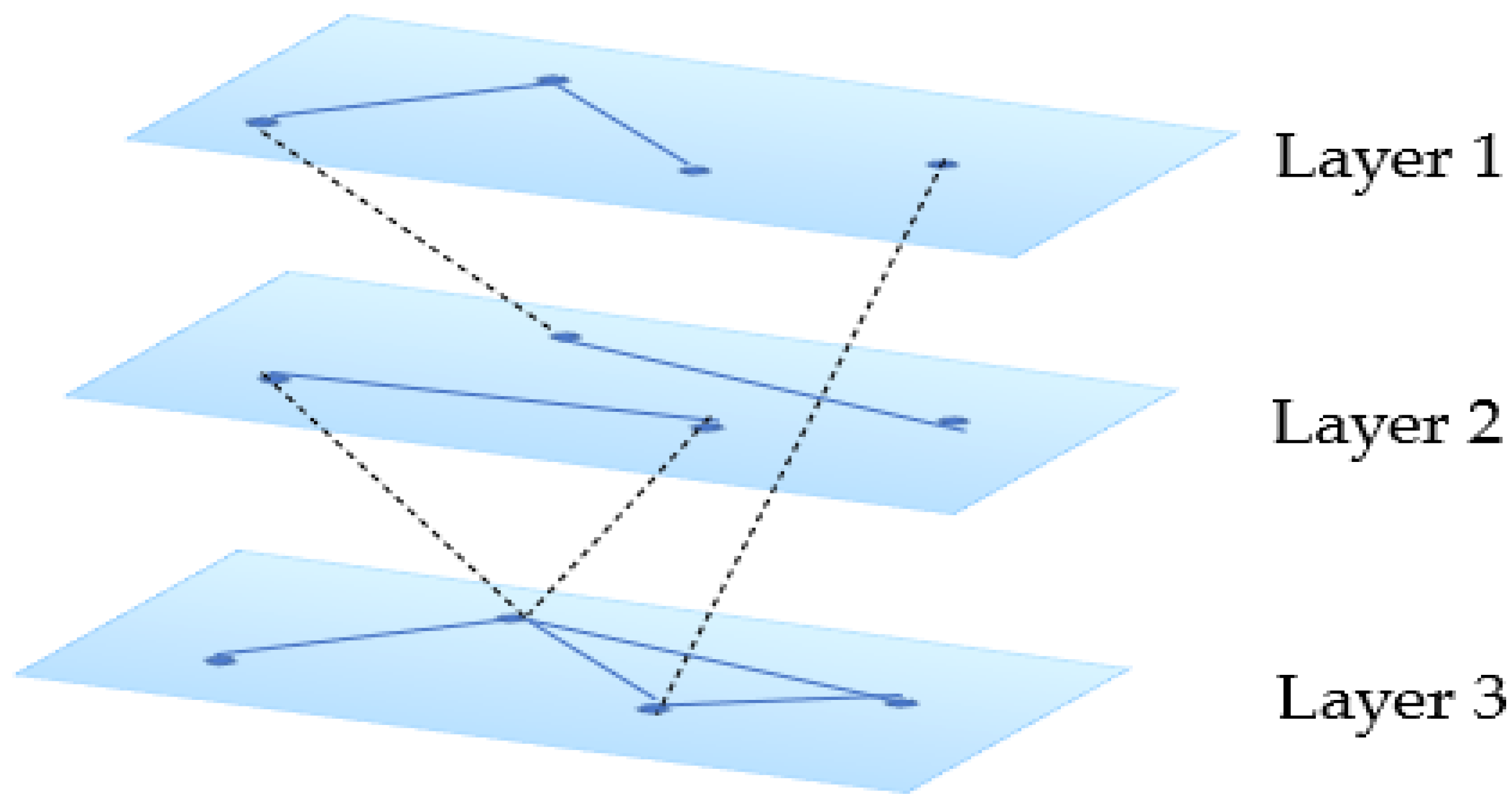
Connections between actors in a single time series class are determined by analyzing the networks constructed by DTW-weighting edges. However, when evaluating the relationships between countries from various time series, distinct layers for each connection are formed. With the time series used to define this layer, a network family consisting of weighted networks, namely multiplex systems, is generated. Such systems have multiple subsystems and layers of connectivity, and it is critical to consider such “multiplex” features when attempting to improve the understanding of complex systems. As a result, it is necessary to generalize “traditional” network theory by creating a framework and associated tools for thoroughly studying multiplex systems. Structures with layers (besides nodes and edges) are used to represent systems consisting of networks at multiple levels or with multiple edge types (or similar properties). It is recommended to start with the most general structure and later introduce relevant limitations to yield existing notions of multiplex networks. In a standard multiplex network framework, each node can belong to any subset of layers and can consider edges covering binary connections between all possible node and layer combinations. Consequently, any node from any layer could be connected to any node from another layer. Figure 1 displays a multiplex model with different layers.

We must define connections between pairs of node-layer tuples in a multiplex network. The term “adjacency” will be used to describe a direct connection between two node-layers via an edge, and the term “incidence” will be used to describe the connection between a node-layer and an edge. In this sense, two edges that are incident to the same node-layer are also “incident” themselves. We will allow any type of edge that can occur between any pair of node-layers, including those where a node is adjacent to a copy of itself in another layer, and those where a node is adjacent to another node from another layer.

We must define a sequence $L={\left\{L_a\right\}}_{a=1}^d$ of sets of elementary layers such that there is only one set of such layers, because a multilayer network can have any number $d$ of aspects. Each aspect $a$ has its own $L_a$. By assembling a set of all the combinations of elementary layers using a Cartesian product $L_{1}x{L}_{2}x\dots x{L}_d$, we can construct a set of layers in a multilayer network using the sequence of sets of elementary layers. We want to allow nodes to be missing in some layers. Hence, for each node and layer combination, we indicate whether the node belongs to that layer. We first create a set $Vx{L}_{1}x{L}_{2}x\dots x{L}_d$ of all combinations and then define a subset $V_M\subset Vx{L}_{1}x{L}_{2}x\dots x{L}_d$ that only contains node-layer combinations with a node in the corresponding layer. To refer to a node that exists on a specific layer, we will frequently use the term node-layer tuple (i.e., “node-layer”). As a result, the node-layer of node $u$, $\left(u,{\alpha }_1,{\alpha }_2,\dots ,{\alpha }_d\right)$ represents node $u$ on layer $\left({\alpha }_1,{\alpha }_2,\dots ,{\alpha }_d\right)$.

Adjacencies in normal networks (i.e., graphs) are defined by an edge set $E\subset VxV$, where the first element in each edge is the starting node and the second element is the ending node. We must also specify the starting and ending layers for each edge in multiplex networks. As a result, we define an edge set $E_M$ of a multiplex network as a set of pairs of possible node and elementary layer combinations: $E_M\subset V_{M}x{V}_M$.

Using the abovementioned components, we define a multiplex network as a quadruplet $M=\left(V_M,E_M,V,L\right)$. If the number of aspects is zero $\left(d=0\right)$, the multiplex network M becomes a monoplex (i.e., single-layer) network. In that case, $V_M=V$, making the set $V_M$ obsolete. Because the first two elements of a multiplex network $M$ produce a graph $G_M=\left(V_M,E_M\right)$, a multiplex network can be represented as a graph with labelled nodes. Dependencies among financial time series can be described using various measures, which has led to the study of various types of networks (e.g., correlation networks, causality networks). In the literature, correlation-based graphs and network filtering tools have been used successfully to model the stock market as a complex system [51]. Because this is a quantity that can be easily and quickly computed, the most common approach uses the Pearson correlation coefficient to define the weight of a link. However, because nonlinearity is an important feature of financial markets [52], the Pearson coefficient measures the linear correlation between two time series. Other measures can provide equally useful information about asset relationships. For example, the Kendall correlation coefficient accounts for monotonic nonlinearity [53,54].

The Kendall correlation coefficient method is easy to implement, general, and scalable, and it does not require ad hoc phase space partitioning, making it suitable for analyzing large, heterogeneous, and non-stationary time series.

In the context of our study, we used multiplex measurements to investigate the relationship dynamics within each country. As a result, weighted, multi-layered network structures were developed and analyzed using time series of the macroeconomic variables. Reciprocal of the dynamic time warping (DTW) values of time series were used in order to assess the degree of similarity between two sub-regions.

Multiplex Structural Measures

In a system consisting of many relationships between its component pieces, when linkages can be identified, edges should be embedded in different layers according to their kind in order to illustrate the system. One should think about an N-node system with M layers that are weighted. An adjacency matrix whose entries are $a_{ij}^{\alpha }$ can be applied to each layer, where $\alpha$ denotes the layer index.

To examine the multiplex structure generated by similarity measures of distinct time series from each nation, it is necessary to specify a number of structural metrics. Each monoplex in the multiplex structure comprises the DTW-weighted edges and the nodes representing different countries. The DTW value determines the strength of weighted edges. In addition to the interaction strength, the strength of a node inside the multiplex topology is also assessed. For that matter, it represents the economic strength or leadership of the nation in question on the macroeconomic market. We measure the strength of a node in a layer as the total of edge weights next to it rather than in terms of degrees. We use $s_i^{\alpha }$ to represent the strength of a node $i$ in the $\alpha$ layer. Furthermore, a node’s weighted edge overlapped degree $o_i$ can be defined as its total strength with $o_i={\displaystyle \sum }_{1\le \alpha \le M}{s}_i^{\alpha }$.

One of the fundamental aspects of a single-layer network is its distribution. In multiplex networks, it is essential to analyze the distribution strength of a node across tiers. It is possible to study the distribution strength of multiple nodes at each tier, but this is not sufficient. In another layer, nodes that function as hubs in one layer may have minimal connections or even exist in isolation. Conversely, nodes that are hubs in one layer are also hubs in the next layer.

As a result, we use $\alpha \in \left\{GDP,GVAD,EX,IMP,FCEH,W,SC,FDII,FDIO,PII,PIO,GFCF\right\}$ in order to obtain the topological strength $s_i$ and the strength of the nodes in each layer $s_i^{\alpha }$.

We calculated the Kendall rank correlation coefficient, ${\tau }_s$, which assesses the similarity of two ranked sequences of data $X$ and $Y$, in order to accurately measure correlations between node strengths. Since it does not assume on the distributions of $X$ and $Y$ and it ranges from −1 to 1, the correlation coefficient ${\tau }_s$ is a nonparametric measure of statistical reliance between two ranks. If $X$ and $Y$ are independent, ${\tau }_s\left(X,Y\right)=0$; if $X$ and $Y$ are identical, ${\tau }_s\left(X,Y\right)=1$; if one rating is precisely the opposite of the other, ${\tau }_s\left(X,Y\right)=-1$. 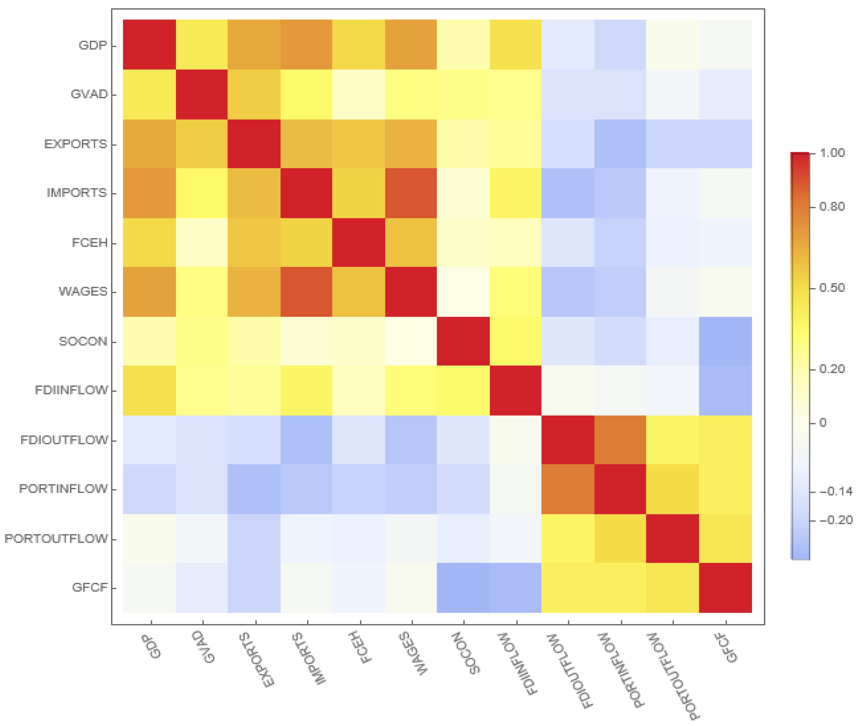Figure 2 shows the ${\tau }_s$ values determined from the rankings of each pair of variables.

Taking into consideration the interaction network that countries have established, network clusters with tight ties to one another become increasingly relevant. This relevance is associated with the aim of facilitating the transfer of vital data inside connection models. In this context, relationships are developed to correctly respond to any crisis or stressful scenario. In contrast to conventional microeconomic models, the influence of any econometric behavior on a system may be described via the variables that comprise the relationships. According to the Kendall rank correlation, the variables in Figure 2 are tightly clustered, as depicted in the histogram. Consequently, the variables gross domestic product, gross value added, final household consumption expenditure, exports, imports, foreign direct investment inflow, social contributions, and wages appeared in a first cluster. The second group included gross fixed capital creation, foreign direct investment outflow, portfolio investment inflow, and portfolio investment outflow.

Clusters created by the Kendall correlation coefficient provide the first clues of variable density. In terms of connection, the impact of countries increases with each successive multiplex layer. From an econometric standpoint, this method elicits information on whether a country dominates the interaction (thus, emerging as leader among other countries) or it shares cooperation-related characteristics with other countries. From a mathematical standpoint, this efficiency can be determined by the power of nodes represented by countries in the multiplex topology. The strength distribution of node $i$ throughout layers may be determined by using the entropy of multiplex strength. The distribution can be analyzed by the entropy measure defined as:

$$H\left(i\right)=-{{\displaystyle \sum }}_{\alpha =1}^M\frac{s_i^{\alpha }}{o_i}\ln \left(\frac{s_i^{\alpha }}{o_i}\right)$$

(3)

for the node $i$. When all linkages of a node are in a single layer, the entropy is zero, and it achieves its maximum value when links are uniformly distributed throughout layers. The higher the $H\left(i\right)$ number, the more uniformly node links are distributed among layers. The multiplex participation coefficient $P\left(i\right)$ of node $i$ may therefore be defined with:

$$P\left(i\right)=\frac{M}{M-1}\left(1-{{\displaystyle \sum }}_{\alpha =1}^M{\left(\frac{s_i^{\alpha }}{o_i}\right)}^2\right).$$

(4)

Multiplex participation coefficient measures the weighted contribution of a node to network communities. Whether the linkages of node $i$ are evenly spread across the $M$ levels or concentrated in only one or few layers is determined by the value of $P\left(i\right)$. The involvement of the node $i$ in the layers of the multiplex is more uniformly distributed, hence the greater the value of $P\left(i\right)$. The average of $P\left(i\right)$ across all nodes is the participation coefficient $P$ for the whole multiplex. The two variables $P\left(i\right)$ and $H\left(i\right)$ express substantially comparable information. The network of isolated nodes leads to an undetermined form of $H\left(i\right)$. Consequently, we only display the $P\left(i\right)$ distributions for the multilayer network taken into consideration (Figure 3). We see the $P\left(i\right)$ distribution in the interval [0.5, 1] although the average participation coefficient of the multiplex is 0.77. This variation shows that there are different node participation rates in each of the network’s twelve layers.

We categorized multiplex nodes by simultaneously evaluating their multiplex participation coefficient and overlapping strength. The former shows how incident edges are distributed across layers, while the latter shows its importance in terms of incident edges. There are three groups based on the multiplex participation coefficient. Focused nodes have a $0<P\left(i\right)<\frac{1}{3}$, mixed nodes have $\frac{1}{3}\le P\left(i\right)<\frac{1}{2}$, and truly multiplex nodes have $P\left(i\right)\ge \frac{2}{3}$. The averages for both areas are practically equal, according to the rank distribution of the participation coefficient. More than two thirds of the participation coefficients are also present. We may conclude that it is advantageous to use multiplexes to evaluate both regions. Besides, we use the corresponding $Z$-score instead of the overlapping strength defined by:

$$z\left(o_i\right)=\frac{o_i-{\mu }_o}{{\sigma }_o},$$

(5)

where ${\mu }_o$ denotes the mean and ${\sigma }_o$ denotes the standard deviation of overlapping strengths. We identify hubs having $z\left(o_i\right)\ge 0.5$ from ordinary nodes having $z\left(o_i\right)<0.5$ based on the Z-score of their overlapping strength. Hence, we may define six types of nodes by considering the multiplex participation coefficient $P\left(i\right)$ of a node and its total overlapping strength $o_i$, as shown in Figure 4, where each node is represented as a point in the $\left(P_i,z\left(o_i\right)\right)$ plane.

Table 6. The multiplex participation coefficient P(i) with Z-scores.

Country	P(i)	z(oi)	Country	P(i)	z(oi)	Country	P(i)	z(oi)
Belgium	0.8015	−0.9836	Cyprus	0.7494	−1.7485	Slovakia	0.8228	0.1712
Bulgaria	0.8023	1.0986	Latvia	0.7885	0.4994	Finland	0.7908	−0.7333
Czech Rep.	0.7906	1.0193	Lithuania	0.7932	0.2756	Sweden	0.8165	−0.4291
Denmark	0.8259	−0.6013	Luxembourg	0.9594	−2.1979	Norway	0.8157	−0.2899
Germany	0.8055	0.3025	Hungary	0.5222	−0.3616	Switzerland	0.7208	−0.5994
Estonia	0.7985	−0.7903	Malta	0.5283	−1.4876	United Kingdom	0.8081	0.1021
Ireland	0.8107	−2.0320	Netherlands	0.6973	−1.5543	Montenegro	0.6298	−0.0517
Greece	0.7142	0.1626	Austria	0.7735	−0.5018	North Macedonia	0.6923	0.4602
Spain	0.7999	0.2090	Poland	0.7969	1.3214	Albania	0.8140	0.4996
France	0.7933	0.0153	Portugal	0.7810	0.5499	Serbia	0.7641	1.1348
Croatia	0.7905	0.6472	Romania	0.7781	1.6844	Turkey	0.7994	1.4379
Italy	0.7929	0.6471	Slovenia	0.7855	0.6876	Bosnia and Herzegovina	0.7789	1.4365

displays the multiplex participation coefficient and the corresponding Z-scores.

It is clear that most countries act as true multiplexes in the multiplex strategy. Only Hungary, Malta, and Montenegro are considered mixed nodes. Moreover, the multiplex model has no focus. It demonstrates the extent to which these countries are linked by various factors.

In addition to the connection architectures in which interactions and cooperation between nations are depicted as nodes, this study also makes statistical measurements of each layer in the multi-layered multiplex structure. These measurements are crucial for a comprehensive analysis of the elements that include each layer. The conditional chance of finding a connection at layer may be expressed as follows if an edge connecting the identical nodes at layer is present as:

$$\mathbb{P}\left(a_{ij}|a{\prime }_{ij}\right)=\frac{{{\displaystyle \sum }}_{ij}{a}_{ij}a{\prime }_{ij}}{{{\displaystyle \sum }}_{ij}{a}_{ij}}.$$

(6)

Figure 5 depicts the conditional probability as a heat map.

The likelihood that edges from a given layer will appear in other layers is displayed in each row of the heat map. The macroeconomic variables wages and social contributions exhibit sparsity with regard to probability. At this point, it is feasible to conclude that these factors are less helpful. The presence of edges and the strength of their connections become crucial when considering the importance of the multiplexes employed in our study. In order to identify which dominant layers have the greatest similarity in node strength, the 1-Wasserstein distances between node strength distributions in each dominant layer are compared (see Figure 6).

The Wasserstein distance matrix reveals that the PII and PIO layers lead to the least similar distributions. Additionally, distance matrix results can be seen in a number of clusters. For instance, the variables GDP, GVAD, EXP, IMP, FCEH, W, and SC frequently group together. Similarly, FDII, FDIO, PII, and PIO form another cluster. However, the 1-Wasserstein distance shows that the second cluster has weaker internal connections.

6. Conclusions and Discussion

Starting from the extant literature on economic growth [55,56,57,58,59,60,61,62,63], we have conducted an investigation on this phenomenon and its evolution using relevant macroeconomic indicators for 36 European countries from the third quarter of 2018 until the third quarter of 2021.

With respect to the methodological approach, we first applied a panel first-difference generalized method of moments with cross-section effects, including all countries. Empirical results supported our four research hypotheses and showed that the phenomenon of economic growth proxied by variables such as gross domestic product, gross value added, financial consumption expenditure of households, and gross fixed capital formation was shaped by numerous factors. More specifically, economic growth values augmented along with imports, exports, and social contributions, thus being in line with various studies in the literature [34,36,39,40]. Overall, the explanatory variables that played a considerable role in the evolution of economic growth across the years were imports, exports, foreign direct investment inflow, foreign direct investment outflow, social contributions, and wages.

Besides the panel data analysis, we also conducted a multiplex network analysis, which explored the connection architectures of 36 countries and yielded statistical measurements for all layers in the multi-layered structure. In this context, we aimed at identifying countries with similar characteristics starting from our macroeconomic variables. Hence, we interpreted matching characteristics as the existence of country cooperation in economic contexts.

Our multiplex network analysis elicited strong clusters of macroeconomic indicators. The first cluster emerged between the variables gross domestic product, gross value added, imports, exports, final consumption and expenditure of households, wages, and social contributions. The second cluster emerged between the variables foreign direct investment inflow, foreign direct investment outflow, portfolio investment inflow, and portfolio investment outflow. After examining the multiplex measurement results, it could be stated that all countries in the sample (except for Hungary, Malta, and Montenegro) have increased cooperation levels during the analyzed period. When cooperation is measured based on the multiplex participation coefficients, we noted that countries such as Romania, Bosnia and Herzegovina, Serbia, Bulgaria, Czech Republic, Slovenia, and Turkey cooperated on the basis of almost all macroeconomic variables. In this sense, it can be observed that Eastern European countries have set a strong cooperation. In terms of countries from Western Europe, the cooperation pattern varied.

Multiplex analysis can be used to demonstrate how similar the countries compared in the model are to one another based on a variety of factors and statistical measurements included in each layer. Such metrics are required for a thorough examination of the elements comprised by each layer. When considering the interaction networks that represent each country, one can state that the relationship between network clusters that are closely related to one another grows over time. Except for Hungary, Malta, and Montenegro, countries increased their level of cooperation during the analyzed period, as shown in Figure 4 and Table 6. Multiplex nodes are classified based on their multiple participation coefficients and overlap degree because the multiplex participation coefficient P(i) provides information about the distribution of event edges among layers. The characteristics of vertices (which represent countries) in any of the three classes determined by the multiplex participation coefficient are similar. Figure 4 depicts the attitudes of Eastern and Western European countries toward cooperation.

With respect to policy implications, we deem that supporting and developing the market economy across all European countries through trade activities (i.e., imports and exports) is an efficient and winning strategy that fuels economic growth. Moreover, an increase in the exporting of high-quality products, technology, and capital is also an important lever for economic growth across Europe. In this sense, R&D transfers and innovations should be supported by public authorities. In addition, stimulating and educating citizens to pay social contributions is another strategy to improve the level of economic growth.

As do all research studies, the present one has its limitations. In the first place, our study examines relationships for the period Q3 2018–Q3 2021. Future studies could consider expanding the time frame and take into account several decades. Secondly, the country sample included 36 European countries. Future research could aim at expanding the country sample by including other nations outside Europe. Moreover, upcoming studies on the factors driving economic growth could focus on comparing different European regions in terms of growth effectiveness or different regions with the European Union. Thirdly, we focused solely on economic variables that play a role in shaping economic growth. Hence, the set of explanatory variables could be expanded as well and include factors related to education, labor utilization and participation, labor mobility, or internet access, which have also driven economic growth, especially in recent years. Finally, despite the fact that multiplex-based network analysis research is predicated on mathematical concepts, comparisons among networks that pertain to separate phenomena or structures should be performed with caution. In multiplexes with varied densities or structures, for instance, centrality assessments generated from macromethods may have variable relevance. Considering ego networks as a micro-approach, we must emphasize that these evaluations must be undertaken within very similar communities or groups. In order to determine the real roots of the knowledge gathered from the mathematical structure, additional in-depth and broad economic investigations are required.