Article

Stochastic Analysis of a Hantavirus Infection Model

by
Yousef Alnafisah
1,* and
Moustafa El-Shahed
2
1
Department of Mathematics, College of Sciences, Qassim University, P.O. Box 6644, Buraydah 51452, Saudi Arabia
2
Department of Mathematics, Unaizah College of Sciences and Arts, Qassim University, P.O. Box 3771, Unaizah 51911, Saudi Arabia
*
Author to whom correspondence should be addressed.
Mathematics 2022, 10(20), 3756; https://doi.org/10.3390/math10203756
Submission received: 7 August 2022 / Revised: 4 October 2022 / Accepted: 8 October 2022 / Published: 12 October 2022

Abstract

:
In this paper, a stochastic Hantavirus infection model is constructed. The existence, uniqueness, and boundedness of the positive solution of the stochastic Hantavirus infection model are derived. The conditions for the extinction of the Hantavirus infection from the stochastic system are obtained. Furthermore, the criteria for the presence of a unique ergodic stationary distribution for the Hantavirus infection model are established using a suitable Lyapunov function. Finally, the importance of environmental noise in the Hantavirus infection model is illustrated using the Milstein method.
MSC:
34D20; 37N25; 92D25; 37A50

1. Introduction

Hantaviruses may be transmitted to humans through the saliva of rodents, such as mice and rats, their urine or feces, or through contact and inhalation of air contaminated with droplets of rodent saliva or dust contaminated with their dry droppings. This may result in fatal diseases in humans, such as pulmonary infection syndrome and hemorrhagic fever. Hantavirus pulmonary infection syndrome is rare, but fatal [1]. The Southwest USA experienced a Hantavirus outbreak in 1993, which led to a high mortality rate. Mathematical modeling of the spread of the Hantavirus infection is one of the important tools for understanding and interpreting different interactions between susceptible and infected mice. A simple mathematical model was developed by Abramson [1] to simulate the propagation of the virus, and it was shown to be capable of simulating some features of infection. In real life, rodents and so-called ‘alien’ species share the resources available in the environment. Therefore, rodents do not only share resources among themselves. Biodiversity and the competition between “alien” species and rodents should be taken into account. According to Peixoto [2] and Solomon [3], biodiversity plays an important role in controlling the spread of Hantavirus. The rodents and nonhost species can exert pressure on one another through the level of their respective interspecific competition. In order to account for the biodiversity effect, Peixoto [2] extended the basic Abramson model by including a nonhost alien species. Yusof et al. [4] extended the Peixoto model to include the effects of harvesting. Some studies of the modeling of Hantavirus infection include [5,6,7,8,9,10,11,12,13,14,15,16,17]. According to [18,19], the intrinsic growth rate, mortality rate, carrying capacity, competition coefficients, and other system parameters would be impacted by environmental changes. Following [20], one can estimate the birth and death rates by an average value plus errors. In general, by the well-known central limit theorem, the error term follows a normal distribution; thus, for a short correlation time, one can assume that the birth and death rates are subjected to the Gaussian white noise. The stochastic effect, which can be significant because the environmental conditions for its transmission are subject to ecological randomness, is not taken into account by the deterministic Peixoto Hantavirus infection model. The primary purpose of this paper is to formulate a stochastic dynamic model to predict Hantavirus infection and identify the key factors that significantly affect the disease spread and control of Hantavirus infection. Hence, our goal in this paper is to provide a comprehensive analysis of the stochastic Hantavirus infection model, especially the existence and uniqueness of a positive global solution and the conditions for the extinction of the Hantavirus infection. This approach has recently been used in many papers for the analysis of stochastic predator-prey systems [21,22,23,24,25], stochastic epidemic models [26,27,28,29,30,31,32,33], and stochastic analysis methods [34,35,36]. This paper is arranged as follows: In Section 3, the existence and uniqueness of a positive global solution of the stochastic Hantavirus infection model are investigated, and sufficient conditions for the extinction of the infection from the stochastic system are obtained. In Section 4, some numerical simulations are presented to verify the obtained theoretical results. Finally, Section 5 contains the conclusion.

2. Hantavirus Model

In this section, we first present Abramson’s model that investigates the spread of Hantavirus infection. In this model, the total population of rodents is divided into susceptible mice x 1 ( t ) and infected mice x 2 ( t ) . The Abramson model’s equations are as follows [1]:
d x 1 d t = b ( x 1 + x 2 ) c x 1 x 1 k ( x 1 + x 2 ) a x 1 x 2 , d x 2 d t = a x 1 x 2 x 2 k ( x 1 + x 2 ) c x 2 ,
where b is the birth rate, c is the death rate, k is related to the carrying capacity of the environment, and a is the constant infection rate. The Peixoto model of competition Hantavirus dynamics including the nonhost alien species x 3 ( t ) takes the form [2]:
d x 1 d t = b ( x 1 + x 2 ) c x 1 x 1 k ( x 1 + x 2 + ρ x 3 ) a x 1 x 2 , d x 2 d t = a x 1 x 2 x 2 k ( x 1 + x 2 + ρ x 3 ) c x 2 , d x 3 d t = ( β γ ) x 3 x 3 k x 3 + δ ( x 1 + x 2 ) ,
where β and γ are the alien population’s birth and death rates, respectively. ρ is the interspecific competition strength exerted by the alien population onto the mouse population, and δ is the interspecific competition strength exerted by the mouse population onto the alien population. In the present paper, the Hantavirus infection model (2) will extend to include the stochastic effects as follows:
d x 1 = b ( x 1 + x 2 ) c x 1 x 1 k ( x 1 + x 2 + ρ x 3 ) a x 1 x 2 d t + σ 1 x 1 d B 1 , d x 2 = a x 1 x 2 x 2 k ( x 1 + x 2 + ρ x 3 ) c x 2 d t + σ 2 x 2 d B 2 , d x 3 = ( β γ ) x 3 x 3 k x 3 + δ ( x 1 + x 2 ) d t + σ 3 x 3 d B 3 ,
where B = B 1 , B 2 , B 3 , t 0 represents the three-dimensional standard Brownian motions. The stochastic extension of the deterministic Abramson model (1) is recovered by setting ρ = 0 and ignoring the third equation of system (3).

3. Dynamics of the Stochastic Model

Firstly, we shall demonstrate the existence and uniqueness of a positive global solution of the Hantavirus infection model (3) in the following theorem.
Theorem 1.
There exists a unique solution of the Hantavirus infection model (3) for positive initial values, and the positive global solution remains in R + 3 with probability one.
Proof. 
Assume ( x 1 ( t ) , x 2 ( t ) , x 3 ( t ) ) is the solution to the Hantavirus infection model (3) for t 0 , τ e , where τ e is the explosion time. Using the following variables
X 1 ( t ) = ln x 1 ( t ) , X 2 ( t ) = ln x 2 ( t ) , X 3 ( t ) = ln x 3 ( t ) ,
one obtains
d X 1 ( t ) = b ( 1 + e X 2 e X 1 ) c 1 k e X 1 + e X 2 + ρ e X 3 a e X 2 σ 1 2 2 d t + σ 1 d B 1 , d X 2 ( t ) = a e X 1 1 k e X 1 + e X 2 + ρ e X 3 c σ 2 2 2 d t + σ 2 d B 2 , d X 3 ( t ) = ( β γ ) 1 k e X 3 + δ ( e X 1 + e X 2 σ 3 2 2 d t + σ 3 d B 3 .
The transformed system (4) has a a unique local solution on 0 , τ e , as the coefficients satisfy the local Lipschitz conditions. Next, we prove that τ e = almost surely. Let s 0 > 0 be sufficiently large for every coordinate in the interval [ 1 s 0 , s 0 ] . For each integer s > s 0 , we can define
τ s = inf t 0 , τ e : min x 1 ( t ) , x 2 ( t ) , x 3 ( t ) ( 1 s , s ) or max x 1 ( t ) , x 2 ( t ) , x 3 ( t ) ( 1 s , s ) .
Using the following positive definite C 2 function V 1 ( x 1 , x 2 , x 3 ) as
V 1 ( x 1 , x 2 , x 3 ) = ( x 1 + 1 ln x 1 ) + ( x 2 + 1 ln x 2 ) + ( x 3 + 1 ln x 3 ) ,
one obtains
d V 1 = [ ( x 1 1 ) b + b x 2 x 1 c 1 k x 1 + x 2 + ρ x 3 a x 2 + ( x 2 1 ) a x 1 1 k x 1 + x 2 + ρ x 3 c + ( x 3 1 ) β γ 1 k ( x 3 + δ ( x 1 + x 2 ) ) + 1 2 i = 1 3 σ i 2 ] d t + σ 1 ( x 1 1 ) d B 1 + σ 2 ( x 2 1 ) d B 2 + σ 3 ( x 3 1 ) d B 3 ( b + 2 + δ k ) x 1 + ( b + a + 2 + δ k ) x 2 + ( β γ + 2 ρ + 1 k ) x 3 + 2 c + 1 2 i = 1 3 σ i 2 d t + σ 1 ( x 1 1 ) d B 1 + σ 2 ( x 2 1 ) d B 2 + σ 3 ( x 3 1 ) d B 3 .
Using the inequality A 2 ( A + 1 ln A ) , for any A > 0 , one obtains
d V 1 [ 2 ( b + 2 + δ k ) ( x 1 + 1 ln x 1 ) + 2 ( b + a + 2 + δ k ) ( x 2 + 1 ln x 2 ) + 2 ( β γ + 2 ρ + 1 k ) ( x 3 + 1 ln x 3 ) + 2 c + 1 2 i = 1 3 σ i 2 ] d t + σ 1 ( x 1 1 ) d B 1 + σ 2 ( x 2 1 ) d B 2 + σ 3 ( x 3 1 ) d B 3 ,
which means that
d V 1 K ( 1 + V 1 ) d t + σ 1 ( x 1 1 ) d B 1 + σ 2 ( x 2 1 ) d B 2 + σ 3 ( x 3 1 ) d B 3 ,
where
K = max 2 ( b + 2 + δ k ) , 2 ( b + a + 2 + δ k ) , 2 ( β γ + 2 ρ + 1 k ) , 2 c + 1 2 i = 1 3 σ i 2 .
Integrating form 0 to t 1 τ s and taking the expectation, one obtains
E V 1 x 1 ( t 1 τ s ) , x 2 ( t 1 τ s ) , x 3 ( t 1 τ s ) V 1 ( x 1 ( 0 ) , x 2 ( 0 ) , x 3 ( 0 ) ) + K T + K 0 t 1 τ s E V 1 d t .
Following [18,37], using Grownwall’s inequality, one obtains
E V 1 x 1 ( t 1 τ s ) , x 2 ( t 1 τ s ) , x 3 ( t 1 τ s ) V 1 x 1 ( 0 ) , x 2 ( 0 ) , x 3 ( 0 ) + K T e K T = K 2 .
The remaining part of the proof is similar to [37,38]; therefore, it can be omitted. □
Theorem 1 shows that the stochastic Hantavirus infection model (3) has a positive global solution remaining in R + 3 with probability one. Next, we establish the boundedness property of the Hantavirus infection model (3).
Theorem 2.
Let H ( t ) = x 1 ( t ) + x 2 ( t ) + x 3 ( t ) ; then, the following inequality holds:
lim t sup E H ( t ) β 1 2 k 2 β 2
almost surely, where β 1 = m a x b , β , and β 2 = m i n c , γ .
Proof. 
According to the stochastic Hantavirus infection model, (3)
d H ( t ) b ( x 1 + x 2 ) c ( x 1 + x 2 ) 1 k ( x 1 + x 2 ) 2 ρ x 3 k ( x 1 + x 2 ) + ( β γ ) x 3 x 3 k ( x 3 + δ ( x 1 + x 2 ) ) d t + σ 1 x 1 d B 1 + σ 2 x 2 d B 2 + σ 3 x 3 d B 3 1 k ( x 1 + x 2 ) 2 b k ( x 1 + x 2 ) + b 2 k 2 4 + b 2 k 4 1 k x 3 2 β k x 3 + β 2 k 2 4 + β 2 k 4 c ( x 1 + x 2 ) γ x 3 + σ 1 x 1 d B 1 + σ 2 x 2 d B 2 + σ 3 x 3 d B 3 β 1 2 k 2 β 2 ( x 1 + x 2 + x 3 ) + σ 1 x 1 d B 1 + σ 2 x 2 d B 2 + σ 3 x 3 d B 3 .
Consequently,
H ( t ) H ( 0 ) + β 1 2 k 2 t β 2 0 t H ( s ) d s + 0 t σ 1 x 1 d B 1 + σ 2 x 2 d B 2 + σ 3 x 3 d B 3 d s .
Using the strong law of large numbers, one obtains
E [ H ( t ) ] H ( 0 ) + β 1 2 k 2 t β 2 0 t E H ( s ) d s .
Consequently,
d E [ H ( t ) ] d t + β 2 E [ H ( t ) ] β 1 2 k 2 .
Thus, one obtains
lim t sup E H ( t ) β 1 2 k 2 β 2 .
According to Theorem 2, the solution of the Hantavirus infection model (3) is uniformly bounded in mean, and as a result, the deterministic Hantavirus infection model (2) is uniformly bounded.
Theorem 3.
If σ 1 2 + 2 b + 1 < 2 c , σ 2 2 + 1 < 2 c , σ 3 2 + 2 β + 1 < 2 γ , then the solutions of (3) are stochastically ultimate bounded.
Proof. 
For ( x 1 ( t ) , x 2 ( t ) , x 3 ( t ) ) R + 3 , we define the following function
V 2 ( x ( t ) , y ( t ) , z ( t ) ) = x ( t ) 2 + y ( t ) 2 + z ( t ) 2 .
By the Itô formula, one has
d V 2 = L V 2 d t + 2 σ 1 x 1 2 d B 1 + 2 σ 2 x 2 2 d B 2 + 2 σ 3 x 3 2 d B 3 ,
where
L V 2 ( x 1 , x 2 , x 3 ) = 2 b x 1 2 + b x 1 x 2 c x 1 2 x 1 2 2 x 1 + x 2 + ρ x 3 a x 1 2 x 2 + a x 1 x 2 2 c x 2 2 x 2 2 2 x 1 + x 2 + ρ x 3 + 2 x 3 2 ( β γ ) 1 k x 3 + δ ( x 1 + x 2 ) + σ 1 2 x 1 2 + σ 2 2 x 2 2 + σ 3 2 x 3 2 ( σ 1 2 + 2 b 2 c + 1 ) x 1 2 + σ 2 2 2 c + 1 x 2 2 + σ 3 2 + 2 ( β γ ) + 1 x 3 2 + 2 a x 1 x 2 2 ( x 1 2 + x 2 2 + x 3 2 ) .
Assume f 1 ( x 1 , x 2 , x 3 ) = ( σ 1 2 + 2 b 2 c + 1 ) x 1 2 + σ 2 2 2 c + 1 x 2 2 + σ 3 2 + 2 ( β γ ) + 1 x 3 2 + 2 a x 1 x 2 2 . According to Theorem 2, one can find that the function f 1 ( x 1 , x 2 , x 3 ) has an upper bound. Let M = sup f 1 ( x 1 , x 2 , x 3 ) + 1 . As a result,
d V 2 = ( M V 2 ) d t + 2 σ 1 x 1 2 d B 1 + 2 σ 2 x 2 2 d B 2 + 2 σ 3 x 3 2 d B 3 .
By the Itô formula, one obtains
d ( e t V 2 ) e t N 1 d t + e t 2 σ 1 x 1 2 d B 1 + 2 σ 2 x 2 2 d B 2 + 2 σ 3 x 3 2 d B 3 .
Consequently,
e t V 2 ( x 1 ( t ) , x 2 ( t ) , x 3 ( t ) ) V 2 ( x 1 ( 0 ) , x 2 ( 0 ) , x 3 ( 0 ) ) + M e t M ;
hence,
lim t sup E [ | X ( t ) | 2 ] M .
According to Chebyshev’s inequality, one obtains
P [ | X ( t ) | η ] E [ | X ( t ) | 2 ] η 2 ,
where η = M ν , ν > 0 . Then,
lim t sup P [ | X ( t ) | η ] M η 2 = ν .
This completes the proof. □
Next, we establish the conditions for the extinction of the Hantavirus infection model (3).
Theorem 4.
For any positive initial conditions, if b < c and β < σ 3 2 2 + γ , then the populations of the Hantavirus infection model (3) will be extinct with probability one.
Proof. 
Using the Itô formula, one obtains
d ( ln ( x 1 + x 2 ) ) = b ( x 1 + x 2 ) k ρ x 3 k c 1 2 ( x 1 + x 2 ) 2 σ 1 2 x 1 2 + σ 2 2 x 2 2 d t + σ 1 x 1 ( x 1 + x 2 ) d B 1 + σ 2 x 2 ( x 1 + x 2 ) d B 2 ( b c ) d t + σ 1 x 1 ( x 1 + x 2 ) d B 1 + σ 2 x 2 ( x 1 + x 2 ) d B 2 .
As a result,
ln x 1 ( t ) + x 2 ( t ) ln x 1 ( 0 ) + x 2 ( 0 ) + ( b c ) t ,
which implies that
lim t sup ln x 1 ( t ) + x 2 ( t ) t b c < 0 a l m o s t s u r e l y .
Hence,
lim t x 1 ( t ) + x 2 ( t ) = 0 .
According to the third equation of the Hantavirus infection system (3), one obtains
d ( ln x 3 ( t ) ) = ( β γ ) 1 k ( x 3 + δ ( x 1 + x 2 ) ) σ 3 2 2 d t + σ 3 d B 3 .
Consequently,
ln x 3 ( t ) = ln x 3 ( 0 ) 1 k 0 t x 3 ( s ) + δ ( x 1 ( s ) + x 2 ( s ) ) d s + ( ( β γ ) σ 3 2 2 ) t + σ 3 B 3 ,
and it follows that
lim t sup ln x 3 ( t ) t ( β γ ) σ 3 2 2 < 0 a l m o s t s u r e l y .
Thus, lim t x 3 ( t ) = 0 . As a result, if b < c , and β < σ 3 2 2 + γ , then the populations of the Hantavirus infection model (3) will be extinct with probability one. □
The asymptotic stability of the Hantavirus infection system (3) is established in the following theorem.
Theorem 5.
For any positive initial conditions, the trivial solution of the Hantavirus infection model (3) is stochastically asymptotically stable in probability if σ 1 2 2 + b < c , σ 3 2 2 + β < γ , and ( σ 1 2 2 + b c ) ( σ 2 2 2 c ) > b 2 4 .
Proof. 
The first step is to consider the following linearized Hantavirus infection model about the origin
d x 1 = ( b c ) x 1 + b x 2 d t + σ 1 x 1 d B 1 , d x 2 = c x 2 d t + σ 2 x 2 d B 2 , d x 3 = ( β γ ) x 3 d t + σ 3 x 3 d B 3 .
Consider the following Lyapunov function
V 3 = 1 2 x 1 2 ( t ) + x 2 2 ( t ) + x 3 2 ( t ) .
One can compute
L V 3 = σ 1 2 2 + b c x 1 2 + σ 2 2 2 c x 2 2 + σ 3 2 2 + β γ x 3 2 + b x 1 x 2 .
One can rewrite L V 3 to be L V 3 = 1 2 X T Q X , where X = ( x 1 , x 2 , x 3 ) and
Q = ( 2 ( σ 1 2 2 + b c ) b 0 b 2 ( σ 2 2 2 c ) 0 0 0 2 ( σ 3 2 2 + β γ ) ) .
The matrix Q will be negative definite if σ 1 2 2 + b < c , σ 3 2 2 + β < γ , and ( σ 1 2 2 + b c ) ( σ 2 2 2 c ) > b 2 4 . As indicated by [39], the linearized stochastic Hantavirus infection model (14) is stochastically stable in the large if L V 3 is a negative-definite function. According to Arnold [40], the trivial solution of the nonlinear stochastic Hantavirus infection model (3) is stochastically asymptotically stable if the linear stochastic Hantavirus model (14) is stochastically asymptotically stable. □
The equilibrium point E = ( x 0 , 0 , 0 ) , where x 0 = k ( b c ) is the Hantavirus-free equilibrium of the deterministic Hantavirus infection model (2), but it may be not an equilibrium of the stochastic Hantavirus infection model (3). Next, we investigate the asymptotic property around E for the stochastic system.
Theorem 6.
The stochastic Hantavirus infection model (3) has the following property
lim t s u p 1 t E 0 t x 1 ( u ) x 0 2 + x 2 ( u ) 2 + x 3 ( u ) 2 d u ( b + x 0 k ) + ( β γ + x 0 ρ k ) β 1 2 k 2 2 β 2 + σ 1 2 2 ( b c ) x 0 k .
Proof. 
In order to prove Theorem 6, one can define the following function
V 4 ( x 1 , x 2 , x 3 ) = x 1 x 0 + ln ( x 1 x 0 ) + x 2 + x 3 .
Applying the Itô formula leads to
d V 4 = ( x 1 x 0 ) b + x 2 x 1 c 1 k ( x 1 + x 2 + ρ x 3 ) a x 2 + x 0 σ 1 2 2 + c x 2 x 2 k ( x 1 + x 2 + ρ x 3 ) + a x 1 x 2 + ( β γ ) x 3 x 3 k x 3 + δ ( x 1 + x 2 ) + σ 1 ( x 1 x 0 ) d B 1 + σ 2 x 2 d B 2 + σ 3 x 3 d B 3 1 k ( x 1 x 0 ) 2 1 k x 2 2 1 k x 3 2 + ( b + x 0 k ) x 2 + ( β γ + x 0 q k ) x 3 + x 0 σ 1 2 2 ( b c ) x 0 d t + σ 1 ( x 1 x 0 ) d B 1 + σ 2 x 2 d B 2 + σ 3 x 3 d B 3 1 k ( x 1 x 0 ) 2 1 k x 2 2 1 k x 3 2 + ( b + x 0 k ) x 2 + ( β γ + x 0 ρ k ) x 3 + x 0 σ 1 2 2 ( b c ) x 0 d t + σ 1 ( x 1 x 0 ) d B 1 + σ 2 x 2 d B 2 + σ 3 x 3 d B 3 .
Consequently,
0 E V 4 x 1 ( t ) , x 2 ( t ) , x 3 ( t ) E V 4 x 1 ( 0 ) , x 2 ( 0 ) , x 3 ( 0 ) + E 0 t 1 k x 1 ( u ) x 0 2 1 k x 2 ( u ) 2 1 k x 3 ( u ) 2 + ( b + x 0 k ) x 2 ( u ) + ( β γ + x 0 ρ k ) x 3 ( s ) + x 0 σ 1 2 2 ( b c ) x 0 d u ,
using Theorem 2, one obtains
E 0 t 1 k x 1 ( u ) x 0 2 + 1 k x 2 ( u ) 2 + 1 k x 3 ( u ) 2 d u E V 4 ( x 1 ( 0 ) , x 2 ( 0 ) , x 3 ( 0 ) ) + ( b + x 0 k ) β 1 2 k 2 β 2 t + ( β γ + x 0 ρ k ) β 1 2 k 2 β 2 t + x 0 σ 1 2 2 ( b c ) x 0 t .
Therefore,
lim t sup 1 t E 0 t x 1 ( u ) x 0 2 + x 2 ( u ) 2 + x 3 ( u ) 2 d u ( b + x 0 k ) + ( β γ + x 0 ρ k ) β 1 2 k 2 2 β 2 + σ 1 2 2 ( b c ) x 0 k .
From Theorem 6, one can see that the Hantavirus infection will tend to die out when the intensity of the stochastic perturbations σ 1 is small enough. In the following theorem, we establish the criteria for the existence of an ergodic stationary distribution in the stochastic Hantavirus infection model (3) using the method of Khasminskii [41]. According to [42,43], one can investigate the stationary distribution for the Hantavirus infection model (3) instead of asymptotically stable equilibria. Before giving the main theorem, we first state the following Lemma
Lemma 1.
([41]). The Markov process X ( t ) has a unique ergodic stationary distribution π ( . ) if there exists a bounded closed domain U 1 R d with regular boundary Γ, having the following properties:
  • H 1 : there is a positive number M 0 such that i , j = 1 d a i j ( x ) η i η j M 0 | η 2 | , x U 1 , η R d ,
  • H 2 : there exists a nonnegative C 2 function V such that L V is negative on R d \ U 1 .
Remark 1.
The positive equilibrium point E = ( x 1 * , x 2 * , x 3 * ) of the deterministic Peixoto system (2) satisfies
( b c ) = 1 k ( x 1 * + x 2 * + ρ x 3 * ) + a x 2 * b x 2 * x 1 * , c = a x 2 * 1 k ( x 1 * + x 2 * + ρ x 3 * ) , ( β γ ) = 1 k x 3 * + δ ( x 1 * + x 2 * ) ,
where
x 1 * = b a , x 2 * = a k ( b c ) b ( 1 ρ δ ) a k ρ ( β γ ) a ( 1 ρ δ ) , x 3 * = k ( β γ ) δ ( b c ) 1 ρ δ ,
0 < ρ < 1 , 0 < δ < 1 , ( β γ ) > δ ( b c ) and β > γ , ( β γ ) > δ ( b c ) , a k ( b c ) > b ( 1 ρ δ ) + a k ρ ( β γ ) .
Theorem 7.
Assume ( a k 1 ) ( 1 ρ ) > δ , ρ + δ + 2 a k ρ < 1 , b > c , β > γ , 0 < ρ δ < 1 , ( β γ ) > δ ( b c ) , a k ( b c ) > b ( 1 ρ δ ) + a k ρ ( β γ ) , and
m < m i n ( a k 1 ) ( 1 ρ ) δ k ( x 1 * ) 2 , a k + a k ρ + 1 k ( x 2 * ) 2 , 1 ρ δ 2 a k ρ k ( x 3 * ) 2 ,
where m = b ( b 2 k 4 c + x 1 * ) + ( a k 1 ) x 1 * σ 1 2 2 + ( a k 1 ) x 2 * σ 2 2 2 + x 3 * σ 3 2 2 ; then, the stochastic Hantavirus infection model (3) has an ergodic stationary distribution for any given positive initial values.
Proof. 
In order to prove Theorem 7, one needs only to validate conditions H 1 and H 2 of Lemma 1. The first step is to validate condition H 1 of Lemma 1. Following [44], one can define the following nonnegative C 2 function
V 5 ( x 1 , x 2 , x 3 ) = α 1 x 1 x 1 * x 1 * ln x 1 x 1 * + α 2 x 2 x 2 * x 2 * ln x 2 x 2 * + α 3 x 3 x 3 * x 3 * ln x 3 x 3 * .
Applying the Itô formula leads to
L V 5 = α 1 ( x 1 x 1 * ) b c + b x 2 x 1 1 k ( x 1 + x 2 + ρ x 3 ) a x 2 + α 2 ( x 2 x 2 * ) a x 1 1 k ( x 1 + x 2 + ρ x 3 ) c + α 3 ( x 3 x 3 * ) β γ 1 k ( x 3 + δ ( x 1 + x 2 ) ) + α 1 x 1 * σ 1 2 2 + α 2 x 2 * σ 2 2 2 + α 3 x 3 * σ 3 2 2 α 1 k ( x 1 x 1 * ) 2 α 2 k ( x 2 x 2 * ) 2 α 3 k ( x 3 x 3 * ) 2 α 1 ( a k + 1 k ) α 2 ( a k 1 k ) ( x 1 x 1 * ) ( x 2 x 2 * ) α 1 ρ k + α 3 δ k ( x 1 x 1 * ) ( x 3 x 3 * ) ρ k ( α 2 + α 3 ) ( x 2 x 2 * ) ( x 3 x 3 * ) + α 1 b ( x 1 x 1 * ) x 2 x 1 x 2 * x 1 * + α 1 x 1 * σ 1 2 2 + α 2 x 2 * σ 2 2 2 + α 3 x 3 * σ 3 2 2 .
Taking α 1 = a k 1 , α 2 = a k + 1 , and α 3 = 1 , therefore,
L V 5 ( a k 1 ) ( 1 ρ ) δ k ( x 1 x 1 * ) 2 a k + a k ρ + 1 k ( x 2 x 2 * ) 2 1 ρ δ 2 a k ρ k ( x 3 x 3 * ) 2 + b ( b 2 k 4 c + x 1 * ) + ( a k 1 ) x 1 * σ 1 2 2 + ( a k + 1 ) x 2 * σ 2 2 2 + x 3 * σ 3 2 2 .
Following [18,44,45,46], when
m < min ( a k 1 ) ( 1 ρ ) δ k ( x 1 * ) 2 , a k + a k ρ + 1 k ( x 2 * ) 2 , 1 ρ δ 2 a k ρ k ( x 3 * ) 2 ,
then the ellipsoid
( a k 1 ) ( 1 ρ ) δ k ( x 1 x 1 * ) 2 a k + a k ρ + 1 k ( x 2 x 2 * ) 2 1 ρ δ 2 a k ρ k ( x 3 x 3 * ) 2 + m = 0 ,
lies entirely in R + 3 . One can take U 1 to be a neighborhood of the ellipsoid, which satisfies U 1 ¯ R + 3 ; hence, L V 5 < 0 for ( x 1 , x 2 , x 3 ) R + 3 \ U 1 ¯ . This implies that the first condition H 1 of the method of Khasminskii [41] is satisfied. The second step is to validate condition H 2 of Lemma 1. The diffusion matrix A 1 of the stochastic Hantavirus infection model (3) is as follows
A 1 = σ 1 2 x 1 2 0 0 0 σ 2 2 x 2 2 0 0 0 σ 3 2 x 3 2 .
Following [37,46,47], we choose M 0 = min σ 1 2 x 1 2 , σ 2 2 x 2 2 , σ 3 2 x 3 2 ; then, one can find a positive number M 0 such that
i , j = 1 3 a i j ( x 1 , x 2 , x 3 ) ξ i ξ j = σ 1 2 x 1 2 ξ 1 2 + σ 2 2 x 2 2 ξ 2 2 + σ 3 2 x 3 2 ξ 3 2 M 0 | ξ 2 | ,
for all ξ = ( ξ 1 , ξ 2 , ξ 3 ) R 3 and ( x 1 , x 2 , x 3 ) U 1 . This implies condition H 2 in Lemma 1 is satisfied. As a result, the stochastic Hantavirus infection model (3) has an ergodic stationary distribution for any given positive initial values. □
Remark 2.
If we assume y ( t ) = x 1 ( t ) + x 2 ( t ) and add the first and second equations of system (3), one obtains
d y ( t ) = ( b c ) y 1 k y 2 ρ y x 3 k d t + σ 1 x 1 d B 1 + σ 2 x 2 d B 2 ( b c ) y ( 1 y k ( b c ) ) d t + σ 1 x 1 d B 1 + σ 2 x 2 d B 2 .
According to Liu and Wang [48], if the intensities of the white noises are sufficiently small and b c > σ 1 2 2 + σ 2 2 2 , then there is a stationary distribution to the following equation for positive initial values
d y ( t ) = ( b c ) y ( 1 y k ( b c ) ) d t + σ 1 y d B 1 + σ 2 y d B 2 ,
and it has an ergodic property. From the third equation of the stochastic Hantavirus infection system (3), one obtains
d x 3 ( t ) ( β γ ) x 3 1 x 3 k ( β γ ) d t + σ 3 x 3 d B 3 ,
According to [49,50], x 3 ( t ) neither reaches zero nor infinity in finite time, and provided ( β γ ) > σ 3 2 2 , the process has been shown to have a stationary distribution. Moreover, it has been shown that
0 < lim t inf x 3 ( t ) lim t sup x 3 ( t ) < a l m o s t s u r e l y .

4. Numerical Simulations

In order to demonstrate the above theoretical results for the stochastic Hantavirus system, we use the following parameters [2,51]:
a = 0.1 ; b = 1 ; c = 0.6 ; β = 1 ; γ = 0.5 ; ρ = 0.2 ; δ = 0.1 ; k = 50 .
To give some numerical finding to the stochastic Hantavirus system (3), we use the Milstein method mentioned in [52,53]. The stochastic Hantavirus infection system (3) reduces to the following discrete system
x 1 ( j + 1 ) = x 1 j + h b ( x 1 j + y 1 j ) c x 1 j x 1 j k ( x 1 j + x 2 j + ρ x 3 j ) a x 1 j x 2 j + σ 1 x 1 j h ϵ 1 j + σ 1 2 2 x 1 j ϵ 1 j 2 1 h x 2 ( j + 1 ) = x 2 j + h a x 1 j x 2 j x 2 j k ( x 1 j + x 2 j + ρ x 3 j ) c x 2 j + σ 2 x 2 j h ϵ 2 j + σ 2 2 2 x 2 j ϵ 2 j 2 1 h x 3 ( j + 1 ) = x 3 j + h ( β γ ) x 3 j x 3 j k x 3 j + δ ( x 1 j + x 2 j ) + σ 3 x 3 j h ϵ 3 j + σ 3 2 2 x 3 j ϵ 3 j 2 1 h ,
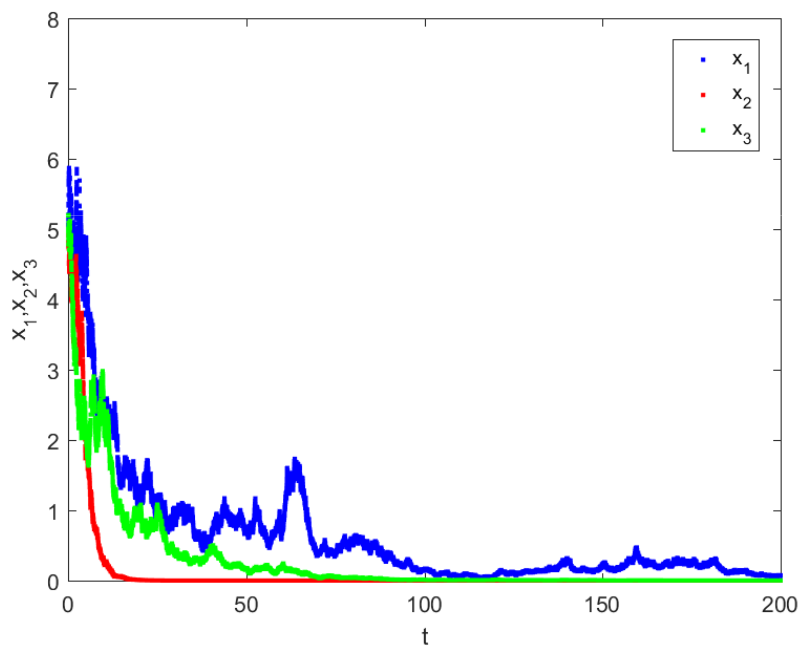
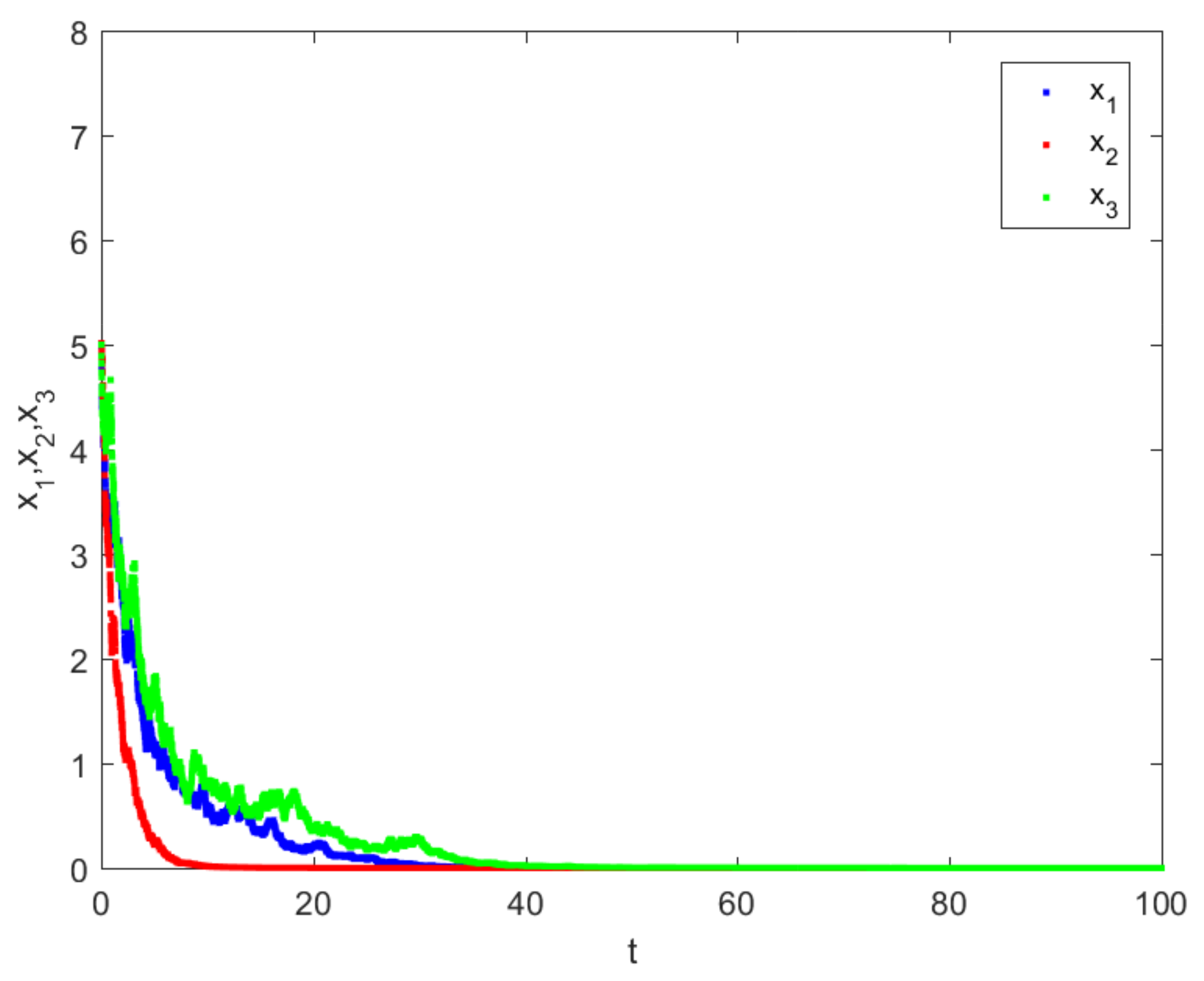
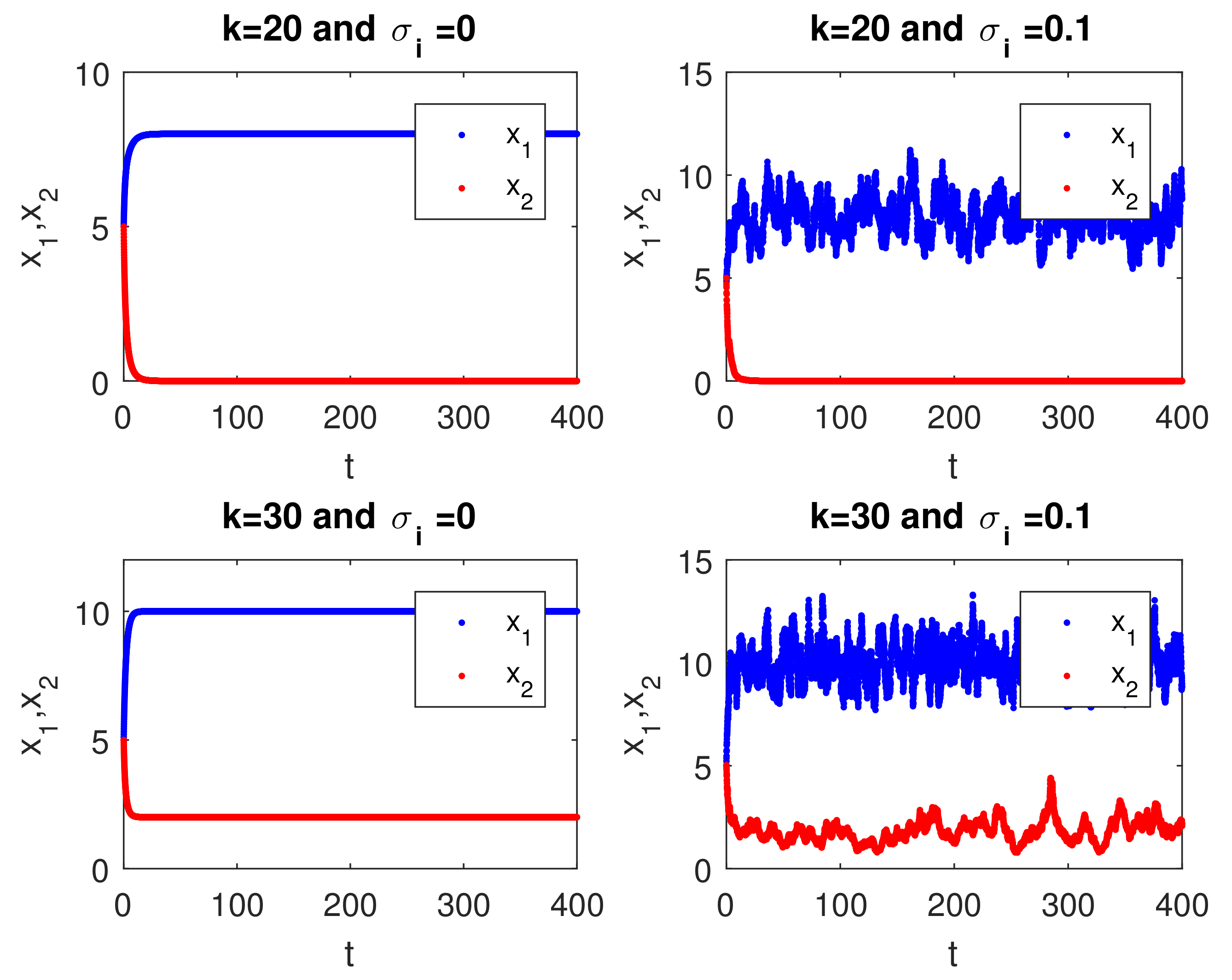
where ϵ i j , ( i , j = 1 , 2 , 3 ) are independent random Gaussian variables N ( 0 , 1 ) , and h is a positive time increment. In the stochastic Hantavirus infection model (3), if one gradually increases the values of σ i and keeps the remaining parameters unchanged, the fluctuations become larger around the positive equilibrium point for the values of σ i = 0.2 , as shown in Figure 1. The infected mice y ( t ) are represented by the black line when ( σ i = 0 ), as seen in Figure 1. The conditions of Theorem 4 for the given parameters are verified, and the populations will be extinct with probability one, if b < c and β < σ 3 3 2 + γ as indicated in Figure 2, when b = 0.55 and β = 0.5 . Moreover, the trivial solution of the Hantavirus infection model (3) is stochastically asymptotically stable in probability if the conditions of Theorem 5 are verified, i.e., σ 1 2 2 + b < c , σ 3 2 2 + β < γ , and ( σ 1 2 2 + b c ) ( σ 2 2 2 c ) > b 2 4 as indicated in Figure 3. The stochastic form of the Abramson model (2) is recovered by setting ρ = 0 and ignoring the third equation of system (3). Following [2,51], there is a critical value k c for the carrying capacity k. The population of the infected y ( t ) will die away when k < k c . The Hantavirus disease will spread and increase in rodents if k > k c . Figure 4 represents the dynamical behavior of the Abramson model (2) and verifies the statement of [1]. For k = 20 , the free Hantavirus equilibrium point E = ( 8 , 0 , 0 ) is locally asymptotically stable in the deterministic model. while the solutions of the stochastic Hantavirus infection model (3) oscillate around the equilibrium point, which coincides with Theorem 6. The oscillation amplitude will be
lim t sup 1 t E 0 t x 1 ( u ) x 0 2 + x 2 ( u ) 2 + x 3 ( u ) 2 d u 80 σ 1 2 + 388 α 2 α 1 2 + 96 .
The histograms of the density function for the Hantavirus infection model (3) are shown in Figure 5, and the system (3) has a unique stationary distribution and has an ergodic property according to the conditions of Theorem 7.

5. Conclusions

This paper mainly analyzed a stochastic Hantavirus infection model. The existence and boundedness of the positive solution of the stochastic Hantavirus infection model were derived. The conditions for the extinction of the Hantavirus infection from the stochastic system were obtained using stochastic analysis tools. Furthermore, the criteria for the presence of a unique ergodic stationary distribution for the Hantavirus infection model were established using a suitable Lyapunov function. The numerical Milstein method was used to simulate the significance of environmental noise in the Hantavirus infection model. When intensities of fluctuation σ i = 0 , one can obtain the results for the deterministic model introduced by Peixoto [2]. One can note that the movement of rodents cannot be neglected; consequently, it is interesting to investigate the spatial effects for the stochastic Hantavirus infection model, which will be future work. Moreover, the authors wish to consider the fractionalization of the stochastic Hantavirus infection model given that there is much current research and example publications in this area, with regard to the SIR model, for example [54]. In future work, the authors wish to conduct a detailed analysis of the stochastic Hantavirus infection model using boundary methods as introduced in the following papers [44,55,56,57,58,59,60,61].

Author Contributions

Data curation, M.E.-S.; Formal analysis, Y.A. All authors have read and agreed to the published version of the manuscript.

Funding

This research received no external funding.

Acknowledgments

The researchers would like to thank the Deanship of Scientific Research, Qassim University, for funding the publication of this project.

Conflicts of Interest

The authors declare no conflict of interest.

References

  1. Abramson, G.; Kenkre, V.M. Spatiotemporal patterns in the Hantavirus infection. Phys. Rev. E 2002, 66, 011912. [Google Scholar] [CrossRef] [PubMed] [Green Version]
  2. Peixoto, I.D.; Abramson, G. The effect of biodiversity on the Hantavirus epizootic. Ecology 2006, 87, 873–879. [Google Scholar] [CrossRef] [Green Version]
  3. Solomon, E.; Berg, L.; Martin, D.W. Biology; Cengage Learning: Boston, MA, USA, 2010. [Google Scholar]
  4. Yusof, F.M.; Mohd, M.H.; Yatim, Y.M.; Ismail, A.I.M. Effects of Biotic Interactions, Abiotic Environments and Harvesting on the Spread of Hantavirus Infection. MATEMATIKA Malays. J. Ind. Appl. Math. 2020, 36, 1–14. [Google Scholar]
  5. Abdullah, F.A.; Ismail, A.I. Simulations of the spread of the Hantavirus using fractional differential equations. Matematika 2011, 27, 149–158. [Google Scholar]
  6. Chen, M.; Clemence, D.P. Analysis of and numerical schemes for a mouse population model in Hantavirus epidemics. J. Differ. Equ. Appl. 2006, 12, 887–899. [Google Scholar] [CrossRef]
  7. Gedeon, T.; Bodelón, C.; Kuenzi, A. Hantavirus transmission in sylvan and peridomestic environments. Bull. Math. Biol. 2010, 72, 541–564. [Google Scholar] [CrossRef]
  8. Allen, L.J.S.; Wesley, C.L.; Owen, R.D.; Goodin, D.G.; Koch, D.; Jonsson, C.B.; Chu, Y.; Hutchinson, J.M.S.; Paige, R.L. A habitat-based model for the spread of Hantavirus between reservoir and spillover species. J. Theor. Biol. 2009, 260, 510–522. [Google Scholar] [CrossRef]
  9. Rida, S.Z.; Abd-elradi, A.S.; Arafa, A.; Khalil, M. The effect of the environmental parameter on the Hantavirus infection through a fractional-order SI model. Int. J. Basic Appl. Sci. 2012, 1, 88–99. [Google Scholar] [CrossRef] [Green Version]
  10. Aguirre, M.A.; Abramson, G.; Bishop, A.R.; Kenkre, V.M. Simulations in the mathematical modeling of the spread of the Hantavirus. Phys. Rev. E 2002, 66, 041908. [Google Scholar] [CrossRef] [Green Version]
  11. Buceta, J.; Escudero, C.; Rubia, F.J.; Lindenberg, K. Outbreaks of Hantavirus induced by seasonality. Phys. Rev. E 2004, 69, 021906. [Google Scholar] [CrossRef] [Green Version]
  12. Karim, M.F.A.; Ismail, A.I.M.; Ching, H.B. Cellular automata modelling of Hantarvirus infection. Chaos Solitons Fractals 2009, 41, 2847–2853. [Google Scholar] [CrossRef]
  13. Abramson, G. The criticality of the Hantavirus infected phase at Zuni. arXiv 2004, arXiv:q-bio/0407003. [Google Scholar]
  14. Goh, S.M.; Ismail, A.I.M.; Noorani, M.S.M.; Hashim, I. Dynamics of the Hantavirus infection through variational iteration method. Nonlinear Anal. Real World Appl. 2009, 10, 2171–2176. [Google Scholar] [CrossRef]
  15. Yusof, F.M.; Abdullah, F.A.; Ismail, A.I. Modeling and optimal control on the spread of Hantavirus infection. Mathematics 2019, 7, 1192. [Google Scholar] [CrossRef] [Green Version]
  16. Moustafa, M.; Mohd, M.H.; Ismail, A.I.; Abdullah, F.A. Dynamical Analysis of a Fractional-Order Hantavirus Infection Model. Int. J. Nonlinear Sci. Numer. Simul. 2019, 21, 171–181. [Google Scholar] [CrossRef]
  17. Moustafa, M.; Abdullah, F.A.; Shafie, S.; Ismail, Z. Dynamical behavior of a fractional-order Hantavirus infection model incorporating harvesting. Alex. Eng. J. 2022, 61, 11301–11312. [Google Scholar] [CrossRef]
  18. Wei, C.; Liu, J.; Zhang, S. Analysis of a stochastic eco-epidemiological model with modified Leslie-Gower functional response. Adv. Differ. Equ. 2018, 2018, 119. [Google Scholar] [CrossRef] [Green Version]
  19. May, R.M. Stability and complexity in model ecosystems. In Stability and Complexity in Model Ecosystems; Princeton University Press: Princeton, NJ, USA, 2019. [Google Scholar]
  20. Liu, M.; Wang, K.; Wu, Q. Survival analysis of stochastic competitive models in a polluted environment and stochastic competitive exclusion principle. Bull. Math. Biol. 2011, 73, 1969–2012. [Google Scholar] [CrossRef]
  21. Xu, C.; Ren, G.; Yu, Y. Extinction analysis of stochastic predator-prey system with stage structure and crowley-martin functional response. Entropy 2019, 21, 252. [Google Scholar] [CrossRef] [Green Version]
  22. Song, G. Dynamics of a stochastic population model with predation effects in polluted environments. Adv. Differ. Equ. 2021, 2021, 189. [Google Scholar] [CrossRef]
  23. Mu, Y.; Lo, W.C. Stochastic dynamics of populations with refuge in polluted turbidostat. Chaos Solitons Fractals 2021, 147, 110963. [Google Scholar] [CrossRef]
  24. Wang, Z.; Deng, M.; Liu, M. Stationary distribution of a stochastic ratio-dependent predator-prey system with regime-switching. Chaos Solitons Fractals 2021, 142, 110462. [Google Scholar] [CrossRef]
  25. Salman, S.; Yousef, A.; Elsadany, A. Dynamic behavior and bifurcation analysis of a deterministic and stochastic coupled logistic map system. Int. J. Dyn. Control 2022, 10, 69–85. [Google Scholar] [CrossRef]
  26. Lei, Q.; Yang, Z. Dynamical behaviors of a stochastic SIRI epidemic model. Appl. Anal. 2017, 96, 2758–2770. [Google Scholar] [CrossRef]
  27. Liu, Q.; Jiang, D.; Hayat, T.; Alsaedi, A.; Ahmad, B. A stochastic SIRS epidemic model with logistic growth and general nonlinear incidence rate. Phys. A Stat. Mech. Its Appl. 2020, 551, 124152. [Google Scholar] [CrossRef]
  28. Li, Q.; Cong, F.; Liu, T.; Zhou, Y. Stationary distribution of a stochastic HIV model with two infective stages. Phys. A Stat. Mech. Its Appl. 2020, 554, 124686. [Google Scholar] [CrossRef]
  29. Khan, A.; Hussain, G.; Yusuf, A.; Usman, A.H.; Humphries, U.W. A hepatitis stochastic epidemic model with acute and chronic stages. Adv. Differ. Equ. 2021, 2021, 181. [Google Scholar] [CrossRef]
  30. Wang, X.; Wang, C.; Wang, K. Extinction and persistence of a stochastic SICA epidemic model with standard incidence rate for HIV transmission. Adv. Differ. Equ. 2021, 2021, 260. [Google Scholar]
  31. Wang, X.; Tan, Y.; Cai, Y.; Wang, K.; Wang, W. Dynamics of a stochastic HBV infection model with cell-to-cell transmission and immune response. Math. Biosci. Eng. 2021, 18, 616–642. [Google Scholar] [CrossRef]
  32. Lan, G.; Yuan, S.; Song, B. The impact of hospital resources and environmental perturbations to the dynamics of SIRS model. J. Frankl. Inst. 2021, 358, 2405–2433. [Google Scholar] [CrossRef]
  33. Ikram, R.; Khan, A.; Zahri, M.; Saeed, A.; Yavuz, M.; Kumam, P. Extinction and stationary distribution of a stochastic COVID-19 epidemic model with time-delay. Comput. Biol. Med. 2022, 141, 105115. [Google Scholar] [CrossRef]
  34. Johari, A.; Khodaparast, A. Analytical stochastic analysis of seismic stability of infinite slope. Soil Dyn. Earthq. Eng. 2015, 79, 17–21. [Google Scholar] [CrossRef]
  35. Gholampour, A.; Johari, A. Reliability analysis of a vertical cut in unsaturated soil using sequential Gaussian simulation. Sci. Iran. 2019, 26, 1214–1231. [Google Scholar] [CrossRef] [Green Version]
  36. Hu, C.; Song, D.; Chen, Z. Analytical stochastic analysis of rock wedge stability using a JDRV method considering the residual factor as a random variable. Geomat. Nat. Hazards Risk 2020, 11, 2079–2094. [Google Scholar] [CrossRef]
  37. Li, L.; Zhao, W. Deterministic and stochastic dynamics of a modified Leslie-Gower prey-predator system with simplified Holling-type IV scheme. Math. Biosci. Eng. 2021, 18, 2813–2831. [Google Scholar] [CrossRef]
  38. Li, J.; Shan, M.; Banerjee, M.; Wang, W. Stochastic dynamics of feline immunodeficiency virus within cat populations. J. Frankl. Inst. 2016, 353, 4191–4212. [Google Scholar] [CrossRef] [Green Version]
  39. Mao, X. Stochastic Differential Equations and Applications; Elsevier: Amsterdam, The Netherlands, 2007. [Google Scholar]
  40. Arnold, L. Stochastic Differential Equations; Wiley: New York, NY, USA, 1974. [Google Scholar]
  41. Khasminskii, R. Stochastic Stability of Differential Equations; Springer Science & Business Media: Berlin/Heidelberg, Germany, 2011; Volume 66. [Google Scholar]
  42. Caraballo, T.; Kloeden, P.E. The persistence of synchronization under environmental noise. Proc. R. Soc. A Math. Phys. Eng. Sci. 2005, 461, 2257–2267. [Google Scholar] [CrossRef]
  43. Ji, C.; Jiang, D.; Liu, H.; Yang, Q. Existence, uniqueness and ergodicity of positive solution of mutualism system with stochastic perturbation. Math. Probl. Eng. 2010, 2010, 684926. [Google Scholar] [CrossRef] [Green Version]
  44. Phan, T.A.; Tian, J.P.; Wang, B. Dynamics of cholera epidemic models in fluctuating environments. Stochastics Dyn. 2021, 21, 2150011. [Google Scholar] [CrossRef]
  45. Li, S.; Wang, X. Analysis of a stochastic predator-prey model with disease in the predator and Beddington-DeAngelis functional response. Adv. Differ. Equ. 2015, 2015, 224. [Google Scholar] [CrossRef] [Green Version]
  46. Huang, Y.; Shi, W.; Wei, C.; Zhang, S. A stochastic predator-prey model with Holling II increasing function in the predator. J. Biol. Dyn. 2021, 15, 1–18. [Google Scholar] [CrossRef]
  47. Chen, Y.; Zhao, W. Dynamical analysis of a stochastic SIRS epidemic model with saturating contact rate. Math. Biosci. Eng. 2020, 17, 5925–5943. [Google Scholar] [CrossRef]
  48. Liu, M.; Wang, K. Stationary distribution, ergodicity and extinction of a stochastic generalized logistic system. Appl. Math. Lett. 2012, 25, 1980–1985. [Google Scholar] [CrossRef] [Green Version]
  49. Alvarez, L.H.; Shepp, L.A. Optimal harvesting of stochastically fluctuating populations. J. Math. Biol. 1998, 37, 155–177. [Google Scholar] [CrossRef]
  50. Lv, J.; Wang, K. Almost sure permanence of stochastic single species models. J. Math. Anal. Appl. 2015, 422, 675–683. [Google Scholar] [CrossRef]
  51. Yusof, F.; Ismail, A.; Ali, N. Effect of predators on the spread of hantavirus infection. Sains Malays. 2014, 43, 1045–1051. [Google Scholar]
  52. Higham, D.J. An algorithmic introduction to numerical simulation of stochastic differential equations. SIAM Rev. 2001, 43, 525–546. [Google Scholar] [CrossRef]
  53. Alnafisah, Y. The implementation of Milstein scheme in two-dimensional SDEs using the Fourier method. In Abstract and Applied Analysis; Hindawi: London, UK, 2018; Volume 2018. [Google Scholar]
  54. Djenina, N.; Ouannas, A.; Batiha, I.M.; Grassi, G.; Oussaeif, T.E.; Momani, S. A Novel Fractional-Order Discrete SIR Model for Predicting COVID-19 Behavior. Mathematics 2022, 10, 2224. [Google Scholar] [CrossRef]
  55. Hening, A.; Nguyen, D.H. Coexistence and extinction for stochastic Kolmogorov systems. Ann. Appl. Probab. 2018, 28, 1893–1942. [Google Scholar] [CrossRef] [Green Version]
  56. Benaim, M. Stochastic persistence. arXiv 2018, arXiv:1806.08450. [Google Scholar]
  57. Phan, T.A.; Tian, J.P. Basic stochastic model for tumor virotherapy. Math. Biosci. Eng. 2020, 17, 4271–4294. [Google Scholar] [CrossRef] [PubMed]
  58. Phan, T.A. Stochastic Modeling for Some Biological and Medical Problems. Ph.D. Thesis, New Mexico State University, Las Cruces, NM, USA, 2020. [Google Scholar]
  59. Phan, T.A.; Tian, J.P. Hopf bifurcation without parameters in deterministic and stochastic modeling of cancer virotherapy, part I. J. Math. Anal. Appl. 2022, 514, 126278. [Google Scholar] [CrossRef]
  60. Phan, T.A.; Tian, J.P. Hopf bifurcation without parameters in deterministic and stochastic modeling of cancer virotherapy, part II. J. Math. Anal. Appl. 2022, 515, 126444. [Google Scholar] [CrossRef]
  61. Phan, T.A.; Wang, S.; Tian, J.P. Analysis of a new stochastic Gompertz diffusion model for untreated human glioblastomas. Stochastics Dyn. 2022, 2022, 2250019. [Google Scholar] [CrossRef]
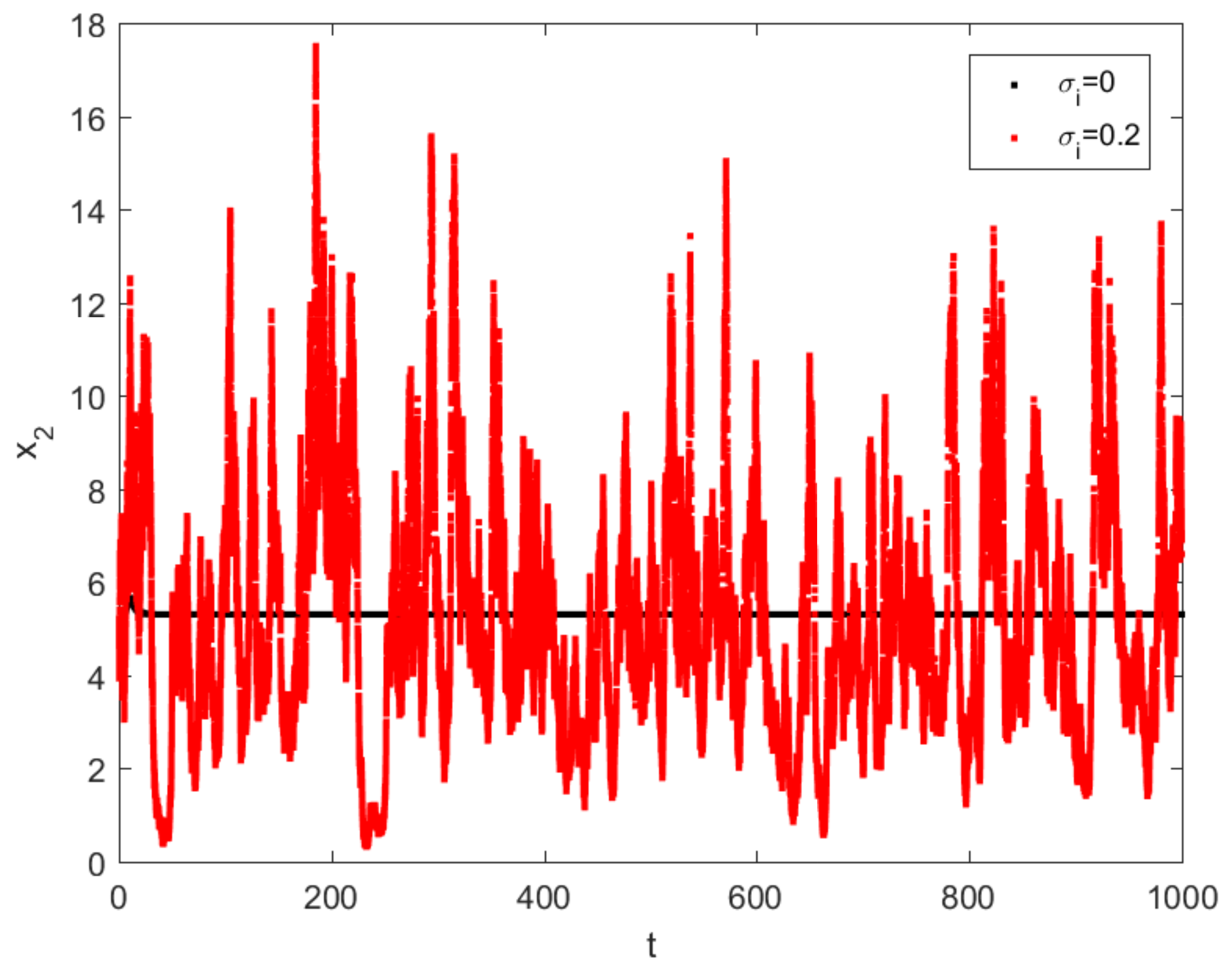
Figure 1. The stochastic Hantavirus system (3) with respect to σ i = 0 and σ i = 0.2 .
Mathematics 10 03756 g001
Figure 2. The extinct behavior of the solutions to the Hantavirus infection system (3).
Mathematics 10 03756 g002
Figure 3. The stochastic trajectories for the trivial solutions of the stochastic Hantavirus infection system (3).
Mathematics 10 03756 g003
Figure 4. The stochastic behavior of the Abramson system for k = 20 , 30 , and σ i = 0 , 0.1 .
Mathematics 10 03756 g004
Figure 5. The density function of susceptible mice of the Hantavirus infection system (3).
Mathematics 10 03756 g005
Publisher’s Note: MDPI stays neutral with regard to jurisdictional claims in published maps and institutional affiliations.