Smooth, Singularity-Free, Finite-Time Tracking Control for Euler–Lagrange Systems

Abstract

This paper investigates the problem of constrained finite-time tracking control of Euler–Lagrange systems subject to system uncertainties and external disturbances. Firstly, we introduce a nonsingular, fast, constrained terminal sliding manifold (NFCTSM) that contains a time-varying gain to deal with the output tracking error constraint. Therefore, the desired performance in steady-state and transience such as ultimate-tracking-error bound, maximum overshoot, and convergence speed are provided. Then, based on the proposed NFCTSM, a smooth adaptive finite-time control is designed such that the tracking errors converge to an arbitrary small region around the origin during a finite period of time. Moreover, the square of the upper bound of the lumped uncertainty is estimated by the adaptive law in order not to use the discontinuous signum function. The efficacy and usefulness of the proposed control methodology are demonstrated via simulation results and comparison with relevant works.

1. Introduction

The problem of control of dynamical systems described by Euler–Lagrange (EL) equations has drawn a lot of consideration since they can be utilized to describe numerous real-world engineering systems, including robot-manipulator systems, spacecraft attitude systems, underwater-vehicle systems, and helicopter systems, to name but a few [1,2,3,4,5,6,7,8,9]. From a practical point of view, it is not straightforward to obtain accurate information of the system, mainly because of the complex structure of the controlled system. Therefore, unknown nonlinearity is generally inevitable and has a negative effect on the system’s performance and even stability [10]. The problem becomes more difficult and challenging as the unknown external disturbance is taken into account. To deal with these disturbing factors and achieve the total disturbance attenuation objective, the sliding-mode control (SMC) approach has attracted considerable attention [11]. The existing conventional SMC laws [12,13] for EL systems utilize a linear sliding manifold and can only result in the asymptotic stability of the closed-loop system, whereas accomplishing tracking control with high accuracy within a finite period of time is of critical importance.

The study of finite-time, trajectory-tracking control for EL systems is usually categorized into two groups: (a) the geometric homogeneity approaches [14,15,16], and (b) the finite-time Lyapunov stabilization methods [17,18]. The first method employs the notion that a homogeneous system is finite-time stable provided that it is asymptotically stable and possesses a negative degree of homogeneity. Because of the inherent uncertainty in the system dynamics, the latter technique has received the attention of many scholars. In SMC, to guarantee that the equilibrium point is finite-time stable, one way is to replace the linear sliding surface with a nonlinear one. For instance, Ref. [19] presents an accurate trajectory tracking-technique with finite-time convergence for robot manipulators that uses nonsingular terminal sliding-mode control (NTSMC), and finite-time Lyapunov stability theory, which is able to deal with uncertain dynamics and unbounded disturbances. In [20], a new type of finite-time sliding-mode controller has been presented for mechanical systems in spite of system uncertainties and external disturbances. To provide the finite-time convergence of trajectories of robot manipulators, an adaptive neural network control has been proposed in [21] such that there is no need to use the joint acceleration signals. The problem of the ${\mathcal{L}}_2$ leader–follower consensus of networked uncertain EL systems guaranteeing finite-time convergence has been investigated in [22]. Using a hyperbolic tangent function, an adaptive SMC-based control for EL systems subject to actuator saturation and external disturbance has been proposed in [23]. By transforming the Lyapunov function into a non-Lipschitz one, a novel adaptive control for robot manipulators has been developed in [24] that ensures finite-time convergence of the system trajectories. Though the problem of finite-time control for robot manipulators has been extensively visited, the behavior of the system trajectory in transient and steady-state responses containing the maximum permitted overshoot and that of the the maximum ultimate tracking error are not taken into account simultaneously. Indeed, they cannot guarantee any specific performance in the transient and steady-state response of the closed-loop system at the same time, which is unacceptable in practice.

In practical applications, because of the safety and physical constraints, the system output or states should be constrained. For instance, to prevent the end effectors of robot manipulators from colliding with obstacles in the environment, they have to work within a specific space. During the recent years, several approaches such as Barrier Lyapunov Function (BLF) [25] and prescribed performance control (PPC) [26] have been employed to achieve certain safety measures and performance requirements in the transient and steady-state responses of EL systems. To provide output constraints of a robot manipulator, a combination of adaptive neural network control and the BLF approach is utilized in [27]. According to the notion of the BLF and NTSMC, the authors of [28] presented a constrained control framework guaranteeing finite-time convergence for the problem of trajectory tracking of robot manipulators. In [29], a novel integral BLF control has been proposed to avoid the violation of output constraints and to enhance the system stability.

Another effective method for satisfying constraints imposed on the system output is the PPC [30]. This control approach has been extensively utilized in various applications, including active suspension systems [31], spacecraft attitude systems [32,33], marine surface vessels [34], and power systems [35], to name but a few. The challenging issue of fault-tolerant control with prescribed performance for uncertain EL systems in the presence of output constraints has been studied in [36]. For EL systems with uncertain dynamics, a combination of finite-time SMC and PPC has been utilized in [37] to develop a constrained control that guarantees the prescribed performance of the tracking error as well as the practically finite-time stability of the full states. The authors in [38] have employed a performance function and a mapping to transform the constrained robot manipulator to the unconstrained one. Then, an adaptive neural control with prespecified performance in both transient and steady-state phases is developed. By virtue of a simple error transformation, an SMC-based constrained attitude control with finite-time convergence for spacecraft has been presented in [39] such that the input saturation and output constraint are satisfied simultaneously. Using the SMC strategy, a control scheme based on the disturbance observer for robot manipulators has been developed in [40], such that the favorable performance of the trajectory tracking error in the transient and steady-state phases are ensured. In [41], to meet the constraints and limitations of the system output as well as the control input of an uncertain robot manipulator, an effective combination of PPC and BLF has been used to achieve tracking control with high accuracy. Despite its satisfactory performance, the design procedure of the above approaches is not straightforward. The main reason is that they are composed of partial derivative terms and complicated functions that result from stabilizing the transformed tracking error.

Motivated by enhancing the existing results and streamlining practical implementations, this work studies the challenging issue of finite-time constrained trajectory tracking control for EL systems subject to the system uncertainty and external disturbance. The principal contributions of this work can be briefly expressed as follows.

• A new constrained sliding surface with finite-time convergence is proposed that possesses two important properties. (1) Compared to the existing nonsingular finite-time SMC controls for the EL systems [42,43], the proposed control strategy has no need for a piecewise continuous function, and a non-singular property is directly achieved that streamlines the stability analysis. (2) Unlike the existing constrained controls for the EL systems using the PPC concept [31,32,33,34,35,36,37,38,39,40,41], the constraint on the system output is considered into the sliding surface as a time-varying gain.
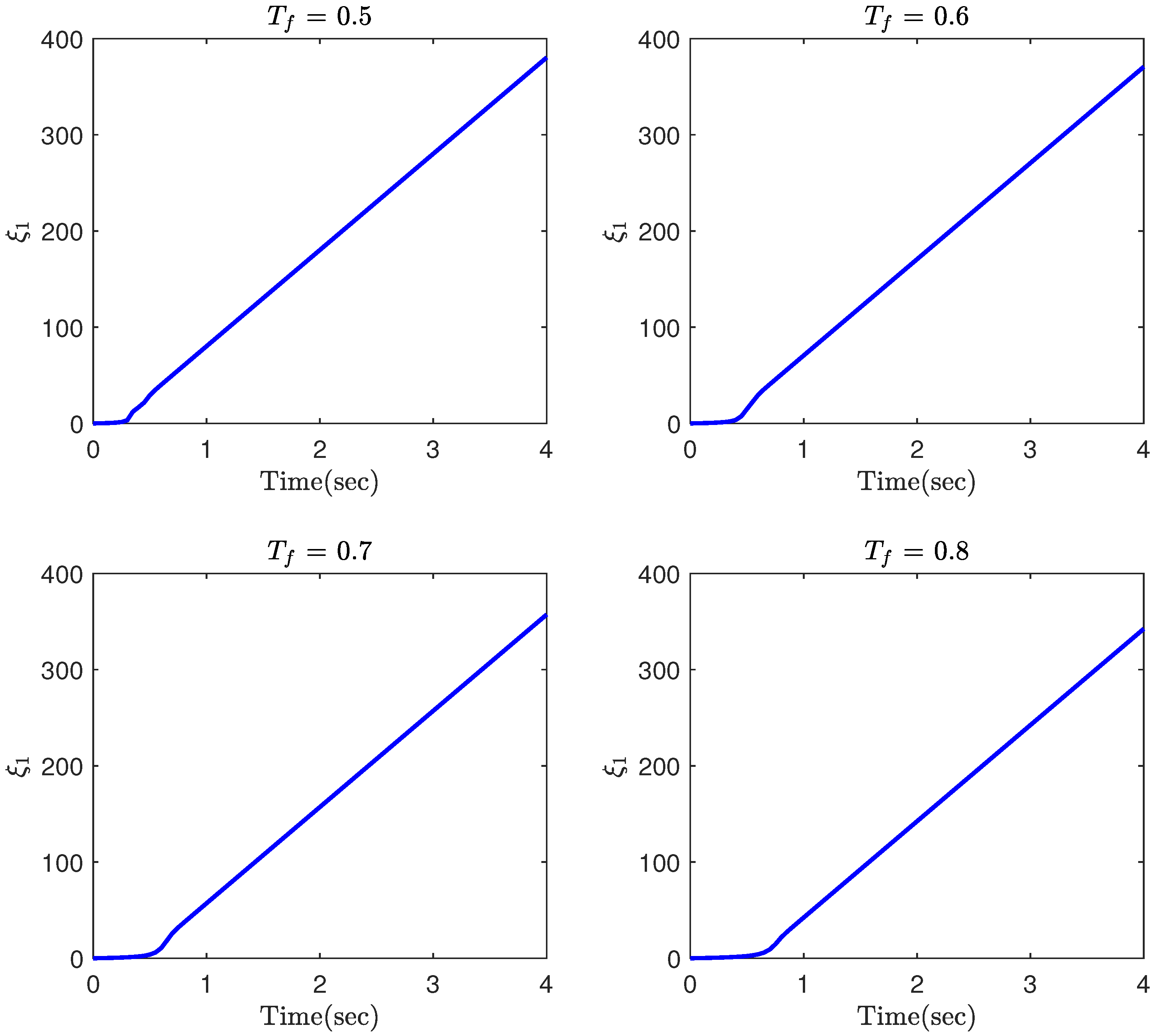
• To deal with the undesired chattering phenomenon as a result of discontinuous sign function, the upper bound of the square of the lumped uncertainty is estimated by the adaptive scheme. Therefore, the discontinuous sign function is effectively removed and a smooth control is achieved.

2. Problem Formulation and Preliminaries

2.1. Dynamics

Consider an n-degree-of-freedom (n-DOF) EL system as

$$M\left(q\right)\ddot{q}+C(q,\dot{q})\dot{q}+G\left(q\right)=u+D,$$

(1)

in the presence of position tracking error constraint expressed as

$$-{\rho }_i\left(t\right)<x_{1i}\left(t\right)<{\rho }_i\left(t\right),$$

(2)

where $q,\dot{q},\ddot{q}\in {\mathbb{R}}^n$ represent the vectors of position, velocity, and acceleration, respectively; $x_1=q-q_d$ denotes the position tracking error with $q_d$ as the desired trajectory; ${\rho }_i\left(t\right)$ shows the time-varying constraint, which will be defined later; $M\left(q\right)\in {\mathbb{R}}^{n\times n}$ is the symmetric positive-definite inertia matrix; $C(q,\dot{q})\in {\mathbb{R}}^{n\times n}$ denotes the Coriolis matrix; $G\left(q\right)\in {\mathbb{R}}^n$ is the vector of gravitational forces; $D\left(t\right)\in {\mathbb{R}}^n$ is the bounded lumped uncertainty as a result of the system uncertainty and external disturbance; and $u\left(t\right)\in {\mathbb{R}}^n$ is the joint control torque vector. Please note that arguments of functions may be dropped hereafter provided that no confusion happens.

Defining $x_1=q-q_d$ and $x_2=\dot{q}-{\dot{q}}_d$, the original dynamical system (1) can be rewritten as

$$\begin{array}{cc}\hfill {\dot{x}}_1& =x_2,\hfill \end{array}$$

(3)

$$\begin{array}{cc}\hfill {\dot{x}}_2& =f(x_1,x_2)-{\ddot{q}}_d+{\tau }_d+\tau ,\hfill \end{array}$$

(4)

where $f(x_1,x_2)=-M^{-1}(x_1+q_d)\left(C(x_1+q_d,x_2+{\dot{q}}_d)(x_2+{\dot{q}}_d)+G(x_1+q_d)\right)$, $\tau =M^{-1}u$, ${\tau }_d=M^{-1}D$, and ${\parallel {\tau }_d\parallel }^2\le \theta$, with $\theta$ being a positive constant.

2.2. Preliminaries

Lemma 1.

For any given scalars ${\alpha }_1>0$, ${\alpha }_2>0$, $0<\beta <1$, a Lyapunov condition for finite-time stability is provided as $\dot{V}\left(t\right)\le -{\alpha }_{1}V\left(t\right)-{\alpha }_2{V}^{\beta }\left(t\right)$, for which the convergence time can be calculated as $T_s=t_0+\frac{1}{{\alpha }_1(1-\beta )}ln\frac{{\alpha }_1{V}^{1-\beta }\left(t_0\right)+{\alpha }_2}{{\alpha }_2}$ [1].

Lemma 2.

Consider the nonlinear system $\dot{x}=f\left(x\right)$ [44]. If there exists a continuous positive-definite function $V\left(t\right)$, real numbers ${\alpha }_1>0$, ${\alpha }_2>0$, $0<\beta <1$, and $0<\eta <\infty$, such that $\dot{V}\left(x\right)\le -{\alpha }_{1}V\left(x\right)-{\alpha }_2{V}^{\beta }\left(x\right)+\eta$, then the trajectories of the nonlinear system $\dot{x}=f\left(x\right)$ is practical finite-time stable and the convergence region can be described as

$$\{\underset{t\to T_r}{lim}|V\left(x\right)\le min\{\frac{\eta }{(1-{\theta }_0){\alpha }_1,},{\left(\frac{\eta }{(1-{\theta }_0){\alpha }_2}\right)}^{\frac{1}{\beta }}\}\}$$

where ${\theta }_0$ satisfies $0<{\theta }_0<1$. The convergence time is given by

$$T_r\le max\{t_0+\frac{1}{{\theta }_0{\alpha }_1(1-\beta )}ln\frac{{\theta }_0{\alpha }_1{V}^{1-\beta }\left(t_0\right)+{\alpha }_2}{{\alpha }_2},t_0+\frac{1}{{\alpha }_1(1-\beta )}ln\frac{{\alpha }_1{V}^{1-\beta }\left(t_0\right)+{\theta }_0{\alpha }_2}{{\theta }_0{\alpha }_2}\}.$$

Definition 1.

The function $\rho \left(t\right)$ is called the finite-time presribed performance function (FTPPF) provided that [45] (1) $\rho \left(t\right)>0$, (2) $\dot{\rho }\left(t\right)\le 0$, (3) ${lim}_{t\to T_f}\rho \left(t\right)={\rho }_T>0$, and (4) $\rho \left(t\right)={\rho }_T$ for any $t\ge T_f$, where ${\rho }_T$ and $T_f$ are positive scalar and convergence time, respectively, which can be selected as arbitrarily small.

Based on this performance function, any desired performance characteristics of the tracking error, including convergence rate, maximum allowable overshoot, and maximum steady-state error bound can be achieved a priori. The function below having the aforementioned properties in Definition 1 could be defined as a potential FTPPF [32]

$$\rho \left(t\right)=\left\{\begin{array}{cc}{\left({\rho }_0^{\kappa }-\kappa \lambda t\right)}^{\frac{1}{\kappa }}+{\rho }_T,\hfill & 0\le t<T_f,\hfill \\ {\rho }_T,\hfill & t\ge T_f.\hfill \end{array}\right.$$

(5)

in which $T_f$ and ${\rho }_T$ denote the settling time and maximum steady-state error value, respectively. The real numbers ${\rho }_0$, $\kappa$, and $\lambda$ are suitably selected based on $T_f$, ${\rho }_T$, and the initial value of the performance function. Moreover, ${\rho }_0=\rho \left(0\right)-{\rho }_T$, $\lambda =\frac{{\rho }_0^{\kappa }}{\kappa T_f}$, and $\kappa =\frac{a_1}{a_2}\in (0,1)$, where $a_1$ and $a_2$ denote positive odd and even integers, respectively.

2.3. Control Objective

The main control objective of the present work is to develop a constrained finite-time control framework for the nonlinear EL system described by Equations (3) and (4) such that the time-varying reference trajectory is tracked by the output. More specifically, the control objectives could be described as follows:

1.

The system output follows the reference trajectory within a finite time.

2.

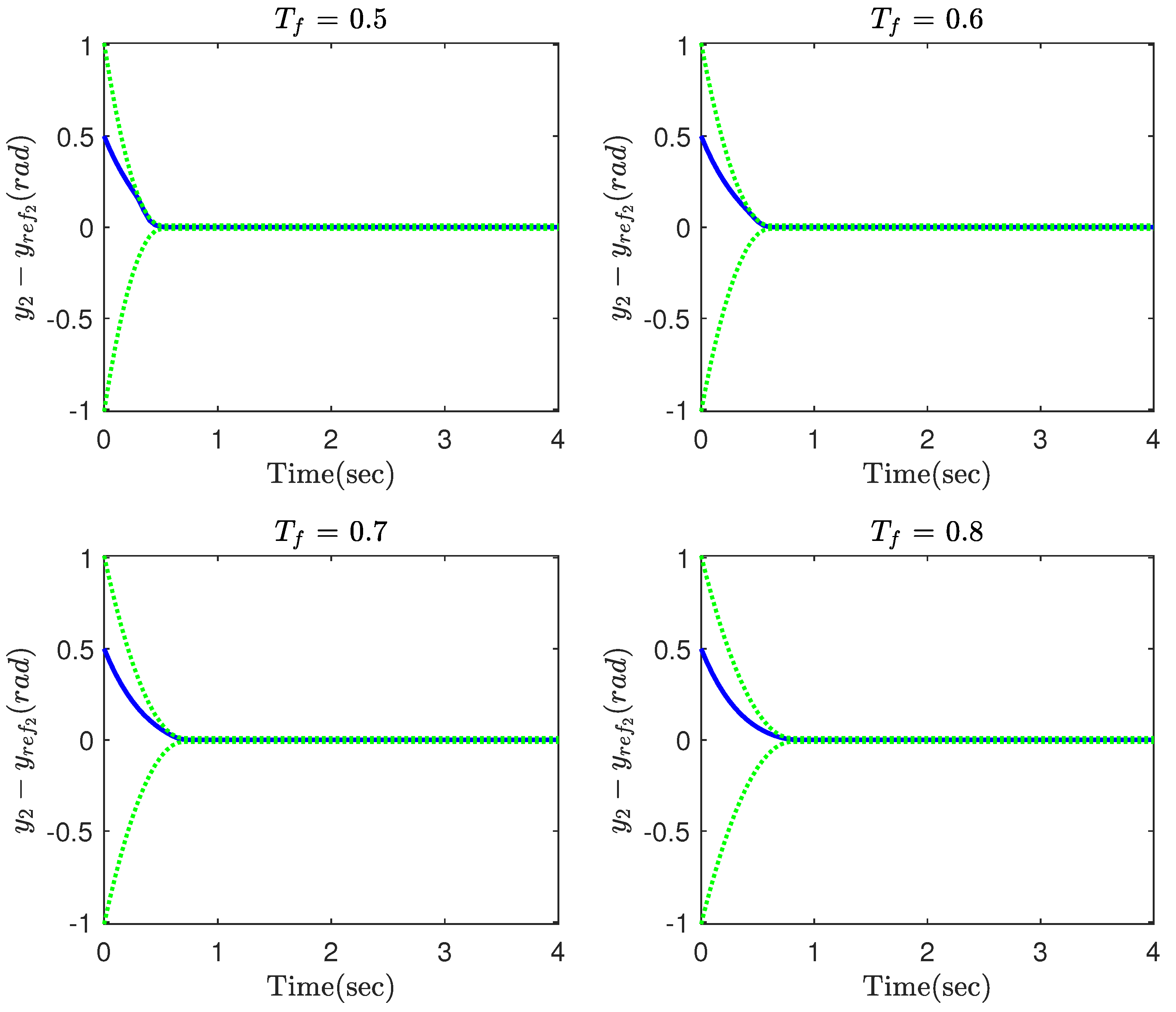
The prescribed performance of the system output is obtained via a performance function in which neither complicated terms nor tedious control parameters regulation are required.

3. Main Results

To achieve the aforementioned control objectives, an adaptive smooth singularity-free control scheme with finite-time convergence is developed. To this end, a nonsingular fast constrained terminal sliding manifold (NFCTSM) is introduced. A special property of the proposed NFCTSM is that it contains a time-varying gain to deal with the output tracking error constraint. Based on the proposed NFCTSM, a smooth singularity-free adaptive finite-time control is designed such that the tracking errors converge to an arbitrary small region around zero in finite time. Moreover, the square of the upper bound of the total uncertainty is estimated by the adaptive law in order not to use the discontinuous signum function.

3.1. Nonsingular Fast Constrained Terminal Sliding Manifold (NFCTSM)

Let us define a NFCTSM as $S\left(t\right)={[S_1\left(t\right),\dots ,S_n\left(t\right)]}^T\in {\mathbb{R}}^n$ with

$$\begin{array}{c}\hfill S_i\left(t\right)=x_{1i}\left(t\right)+{\left(\frac{1}{k_{2i}}\right)}^{\frac{1}{{\gamma }_1}}{\lfloor x_{2i}\left(t\right)+(k_{1i}+{\xi }_i\left(t\right))x_{1i}\left(t\right)\rceil }^{\frac{1}{{\gamma }_1}},\end{array}$$

(6)

where $K_1=\mathrm{diag}(k_{11},\dots ,k_{1n})$, $K_2=\mathrm{diag}(k_{21},\dots ,k_{2n})$ are positive-definite matrices, $0<{\gamma }_1<1$, $\xi =\mathrm{diag}({\xi }_1,\dots ,{\xi }_n)$ with ${\xi }_i\left(t\right)={\int }_0^t{\left(\frac{{\varphi }_i\left(v\right)}{1-{\varphi }_i\left(v\right)\left|x_{1i}\left(v\right)\right|}\right)}^{2}dv$, and ${\varphi }_i\left(t\right)=\frac{1}{{\rho }_i\left(t\right)}$. Moreover, ${\lfloor x_{1i}\rceil }^v=\left[\right|x_{11}{|}^{{\gamma }_1}sgn\left(x_{11}\right),\dots ,|x_{1n}{{|}^{{\gamma }_1}sgn\left(x_{1n}\right)]}^T$ in which $sgn(·)$ is the sign function. When $S_i\left(t\right)=0$ is achieved, it can be easily proved that (please refer to Appendix A)

$$\begin{array}{c}\hfill {\dot{x}}_{1i}\left(t\right)=-(k_{1i}+{\xi }_i\left(t\right))x_{1i}-k_{2i}{\lfloor x_{1i}\left(t\right)\rceil }^{{\gamma }_1}.\end{array}$$

(7)

Theorem 1.

When $S_i\left(t\right)=0$ is reached, the output tracking errors converge to the origin in a finite time and the prescribed performance on $x_1$ is achieved.

Proof. 

Construct a Lyapunov function candidate as

$$V_1\left(t\right)=\frac{1}{2}\sum _{i=1}^n{x}_{1i}^2.$$

Differentiating $V_1\left(t\right)$ with respect to time provides

$$\begin{array}{cc}\hfill {\dot{V}}_1\left(t\right)& =\sum _{i=1}^n{x}_{1i}{\dot{x}}_{1i}=-\sum _{i=1}^n(k_{1i}+{\xi }_i)|x_{1i}{|}^2-\sum _{i=1}^n{k}_{2i}{\left|x_{1i}\right|}^{1+{\gamma }_1}\hfill \\ \hfill & \le -{\overline{k}}_1{V}_1-{\overline{k}}_2{V}_1^{\overline{{\gamma }_1}}.\hfill \end{array}$$

(8)

where ${\overline{k}}_1=2min\left\{k_{1i}\right\}$, ${\overline{k}}_2=2^{\frac{1+{\gamma }_1}{2}}min\left\{k_{2i}\right\}$, and $\overline{{\gamma }_1}=\frac{1+{\gamma }_1}{2}$. If $|x_{1i}\left(0\right)|<|\rho \left(0\right)|$, then the time-varying gain ${\xi }_i\left(t\right)$ is positive. Moreover, based on Lemma 1, it is inferred that $x_{1i}$ and $x_{2i}$ converge to the origin within a finite time calculated as

$$\begin{array}{c}\hfill T_{s,1}=\frac{1}{{\overline{k}}_1(1-\overline{{\gamma }_1})}ln\frac{{\overline{k}}_2+{\overline{k}}_1{V}^{1-\overline{{\gamma }_1}}\left(0\right)}{{\overline{k}}_2}.\end{array}$$

(9)

The proof is finished here. □

3.2. Finite-Time Tracking Control

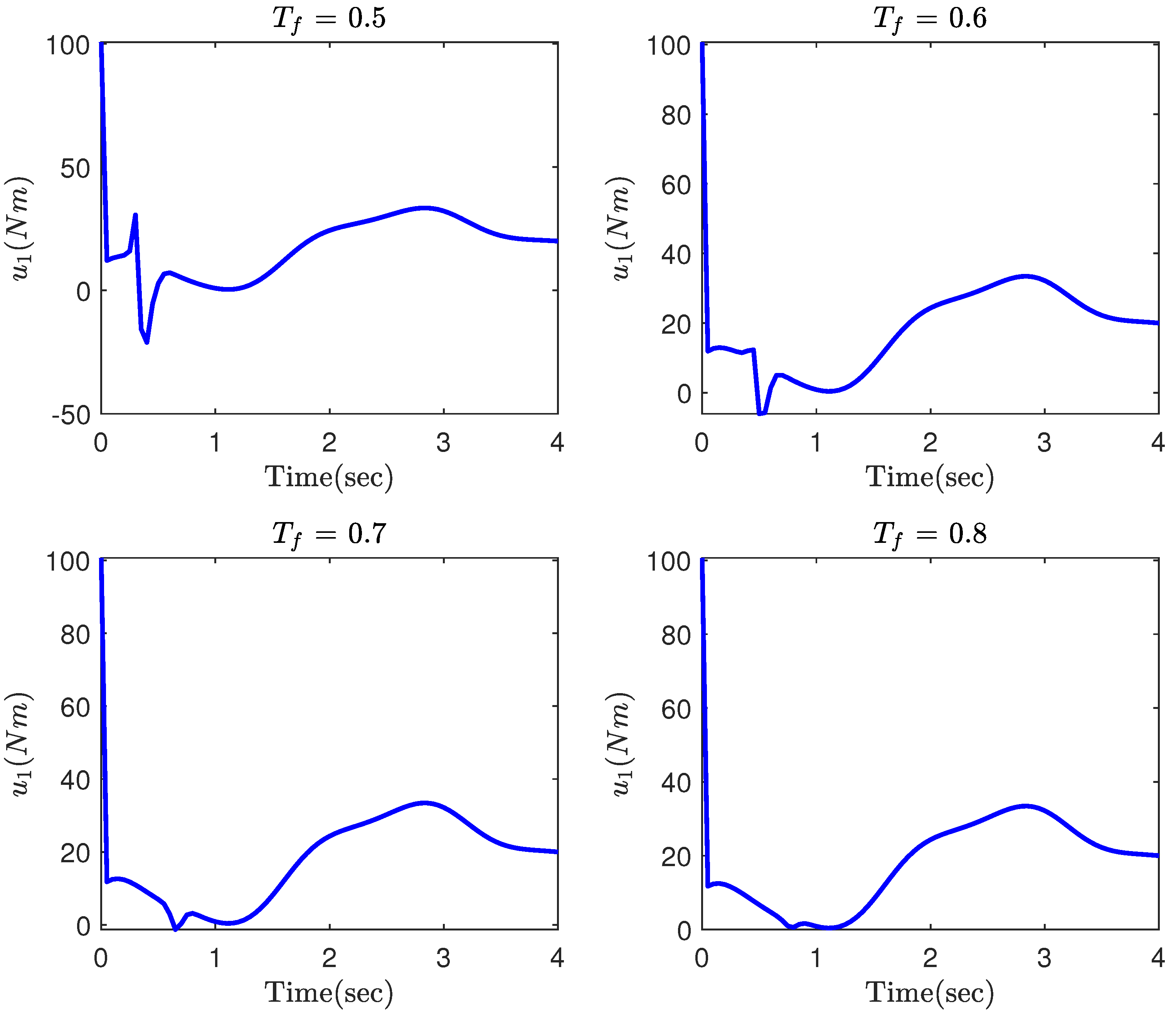
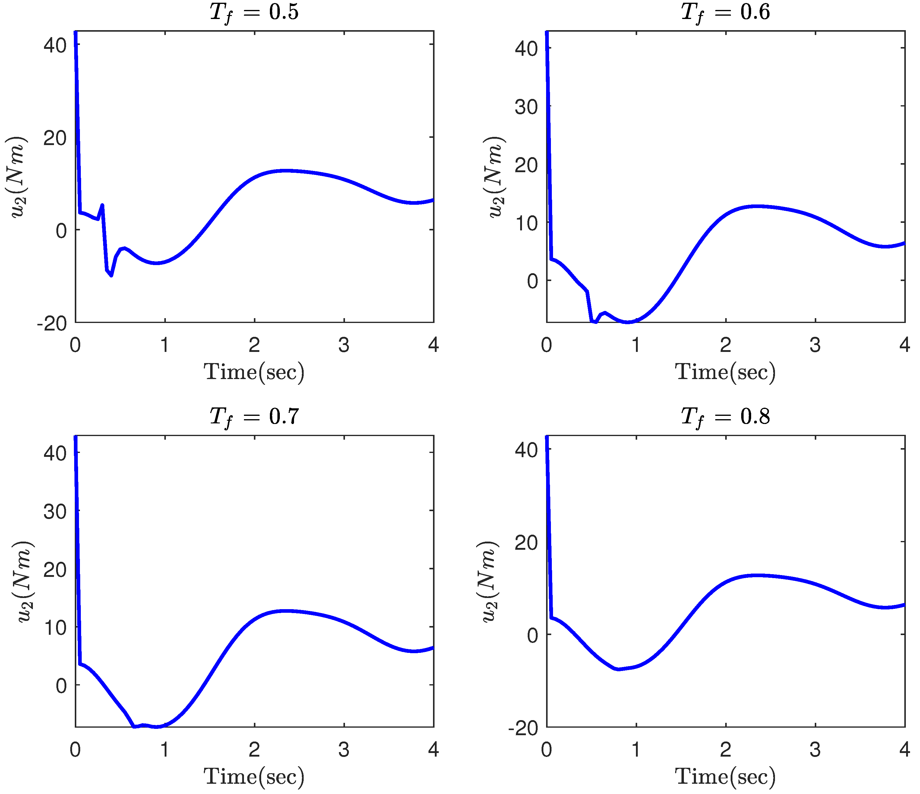
Taking time-derivative of the NFCTSM (6)

$$\begin{array}{cc}\hfill \dot{S}& =x_2+\frac{1}{{\gamma }_1}{\left(K_2\right)}^{\frac{1}{{\gamma }_1}}\mathrm{diag}\left(|x_{2i}+(k_{1i}+{\xi }_i)x_{1i}{|}^{\frac{1}{{\gamma }_1}-1}\right)\left({\dot{x}}_2+(K_1+\xi )x_2+\dot{\xi }{x}_1\right)\hfill \\ \hfill & =x_2+\frac{1}{{\gamma }_1}{\left(K_2\right)}^{\frac{1}{{\gamma }_1}}\mathrm{diag}\left(|x_{2i}+(k_{1i}+{\xi }_i)x_{1i}{|}^{\frac{1}{{\gamma }_1}-1}\right)\left(f-{\ddot{q}}_d+{\tau }_d+\tau +(K_1+\xi )x_2+\dot{\xi }{x}_1\right)\hfill \end{array}$$

(10)

With a simple manipulation, Equation (10) can be simplified as

$$\begin{array}{c}\hfill \dot{S}=\mathsf{\Lambda }\left({\rm Y}+\tau +{\tau }_d\right)-K_{1}S,\end{array}$$

(11)

where $\mathsf{\Lambda }=\mathrm{diag}({\mathsf{\Lambda }}_1,{\mathsf{\Lambda }}_2,{\mathsf{\Lambda }}_3)$ with ${\mathsf{\Lambda }}_i=\frac{1}{{\gamma }_1}{\left(k_{2i}\right)}^{\frac{1}{{\gamma }_1}}{\left|x_{2i}+(k_{1i}+{\xi }_i)x_{1i}\right|}^{\frac{1}{{\gamma }_1}-1}$, $i=1,2,3$, and $\mathrm{Y}=\mathrm{diag}({\mathrm{Y}}_1,{\mathrm{Y}}_2,{\mathrm{Y}}_3)$ with ${\mathrm{Y}}_i={\gamma }_1{k}_{2i}^{-\frac{1}{{\gamma }_1}}{\lfloor x_{2i}+(k_{1i}+{\xi }_i)x_{1i}\rceil }^{2-\frac{1}{{\gamma }_1}}+k_{1i}{\gamma }_1(x_{2i}+(k_{1i}+{\xi }_i)x_{1i})+f-{\ddot{q}}_d+(K_1+\xi )x_2+\dot{\xi }{x}_1$.

Based on Equation (11), the following control law is proposed:

$$\begin{array}{c}\hfill \tau =-\mathrm{Y}-K_{3}S-K_4{\lfloor S\rceil }^{{\gamma }_2}-\frac{\widehat{\theta }}{2{\epsilon }^2}\mathsf{\Lambda }S,\end{array}$$

(12)

where $K_3=\mathrm{diag}(k_{31},\dots ,k_{3n})$, $K_4=\mathrm{diag}(k_{41},\dots ,k_{4n})$ are positive-definite matrices, $0<{\gamma }_2<1$, and $\epsilon$ is a small positive constant. Moreover, the parameter $\widehat{\theta }$ is updated by

$$\begin{array}{c}\hfill \dot{\widehat{\theta }}=p_1\left(\frac{1}{2{\epsilon }^2}{\mathsf{\Lambda }}^2{\parallel S\parallel }^2-p_2\widehat{\theta }\right),\end{array}$$

(13)

where $p_1$ and $p_2$ are two positive constants.

Theorem 2.

Consider the EL system described by (1) with the NFCTSM (6), the finite-time tracking control scheme (12), and the adaptive update law (13). Then, the output tracking errors $x_1$ and $x_2$ will converge to an arbitrary small region around zero during a finite time. Moreover, the prescribed performance for $x_1$ is guaranteed.

Proof. 

Let a Lyapunov function be constructed as

$$\begin{array}{c}\hfill V_2=\frac{1}{2}{S}^{T}S+\frac{1}{2p_1}{\tilde{\theta }}^2,\end{array}$$

(14)

in which $\tilde{\theta }=\theta -\widehat{\theta }$ denotes the estimation error. Taking the time-derivative of $V_2$ and substituting the control input (12) and the adaptive law (13) provides

$$\begin{array}{cc}\hfill {\dot{V}}_2=& S^{T}S-\frac{1}{p_1}\tilde{\theta }\dot{\widehat{\theta }}=S^T\mathsf{\Lambda }\left(-K_{3}S-K_4{\lfloor S\rceil }^{{\gamma }_2}-\frac{\widehat{\theta }}{2\epsilon }\mathsf{\Lambda }S+{\tau }_d\right)-K_1{S}^{T}S\hfill \\ \hfill & -\tilde{\theta }\left(\frac{1}{2{\epsilon }^2}{\mathsf{\Lambda }}^2{\parallel S\parallel }^2-p_2\widehat{\theta }\right)\hfill \\ \hfill \le & -S^T\mathsf{\Lambda }{K}_{3}S-S^T\mathsf{\Lambda }{K}_4{\lfloor S\rceil }^{{\gamma }_2}-S^T{\mathsf{\Lambda }}^{2}S\frac{\widehat{\theta }}{2{\epsilon }^2}+S^T\mathsf{\Lambda }{T}_d-{\mathsf{\Lambda }}^2{\parallel S\parallel }^2\frac{\tilde{\theta }}{2{\epsilon }^2}+p_2\tilde{\theta }\widehat{\theta }\hfill \\ \hfill \le & -S^T\mathsf{\Lambda }{K}_{3}S-S^T\mathsf{\Lambda }{K}_4{\lfloor S\rceil }^{{\gamma }_2}+\frac{{\epsilon }^2}{2}+p_2\tilde{\theta }\widehat{\theta }\hfill \\ \hfill \le & -k_{3min}\sum _{i=1}^n{\mathsf{\Lambda }}_i{S}_i^2-k_{4min}{\left(\sum _{i=1}^n{\mathsf{\Lambda }}_i^2\left|S_i\right|\right)}^{\frac{1+{\gamma }_2}{2}}-\frac{\varpi }{2p_1}{\tilde{\theta }}^2-{\left(\frac{\varpi }{2p_1}{\tilde{\theta }}^2\right)}^{\frac{1+{\gamma }_2}{2}}+{\eta }_1\hfill \end{array}$$

(15)

where ${\eta }_1=\frac{{\epsilon }^2}{2}+\frac{p_2}{2}{\theta }^2-\frac{\varpi }{2p_1}{\tilde{\theta }}^2+{\left(\frac{\varpi }{2p_1}{\tilde{\theta }}^2\right)}^{\frac{1+{\gamma }_2}{2}}$, and $\varpi =\frac{p_1{p}_2}{2}$. Moreover, in the inequality (15), the following inequalities have been utilized:

$$S^T\mathsf{\Lambda }{T}_d\le \frac{1}{2{\epsilon }^2}{\mathsf{\Lambda }}^2{\parallel S\parallel }^2\theta +\frac{{\epsilon }^2}{2}$$

and

$$\tilde{\theta }\widehat{\theta }={\tilde{\theta }}^2-\tilde{\theta }\theta \le \frac{1}{2}{\theta }^2-\frac{1}{2}{\tilde{\theta }}^2.$$

Using the fact that ${\left(\frac{\varpi }{2p_1}{\tilde{\theta }}^2\right)}^{\frac{1+{\gamma }_2}{2}}-\frac{\varpi }{2p_1}{\tilde{\theta }}^2\le 1$, then we have

$$\begin{array}{c}\hfill {\dot{V}}_2\le -{\chi }_1{V}_2-{\chi }_2{V}_2^{{\overline{\gamma }}_2}+{\eta }_2\end{array}$$

(16)

where ${\chi }_1=min\{2k_{3min}{\mathsf{\Lambda }}_i^2,\varpi \}$, ${\chi }_2=min\{2^{\frac{1+{\gamma }_2}{2}}{k}_{4min}{\mathsf{\Lambda }}_i,{\varpi }^{\frac{1+{\gamma }_2}{2}}\}$, ${\overline{\gamma }}_2=\frac{1+{\gamma }_2}{2}$, and ${\eta }_2=\frac{{\epsilon }^2}{2}+\frac{\varpi }{p_1}{\theta }^2+1$. Based on Lemma 2, the system is practically finite-time stable with convergence set given by

$$\begin{array}{c}\hfill \Delta =\{\underset{t\to T_{s,2}}{lim}S|V_2\le min\{(\frac{{\eta }_2}{(1-{\theta }_0){\chi }_1},{(\frac{{\eta }_2}{(1-{\theta }_0){\chi }_2})}^{\frac{1}{{\overline{\gamma }}_2}}\}\}\end{array}$$

(17)

where

$$\begin{array}{c}\hfill T_{s,2}\le max\left\{\frac{1}{{\theta }_0{\chi }_1(1-{\overline{\gamma }}_2)}ln\frac{{\theta }_0{\chi }_1{V}_2^{1-{\overline{\gamma }}_2}\left(0\right)+{\chi }_2}{{\chi }_2},\frac{1}{{\chi }_1(1-{\overline{\gamma }}_2)}ln\frac{{\chi }_1{V}_2^{1-{\overline{\gamma }}_2}\left(0\right)+{\theta }_0{\chi }_2}{{\theta }_0{\chi }_2}\right\}.\end{array}$$

(18)

Once the NFCTSM (6) converges to the set $|S_i|\le \Delta$, then one obtains

$$\begin{array}{c}\hfill S_i\left(t\right)=x_{1i}\left(t\right)+{\left(\frac{1}{k_{2i}}\right)}^{\frac{1}{{\gamma }_1}}{\lfloor x_{2i}\left(t\right)+(k_{1i}+{\xi }_i\left(t\right))x_{1i}\left(t\right)\rceil }^{\frac{1}{{\gamma }_1}}={\psi }_i,\left|{\psi }_i\right|\le \Delta \end{array}$$

(19)

which can be equivalently expressed as

$$\begin{array}{c}\hfill {\dot{x}}_{1i}\left(t\right)+\left(k_{1i}+{\xi }_i\left(t\right)-\frac{{\psi }_i}{x_{1i}}\right)x_{1i}+k_{2i}{\lfloor x_{1i}\left(t\right)\rceil }^{{\gamma }_1}=0\end{array}$$

(20)

or

$$\begin{array}{c}\hfill {\dot{x}}_{1i}\left(t\right)+(k_{1i}+{\xi }_i\left(t\right))x_{1i}+\left(k_{2i}-\frac{{\psi }_i}{{\lfloor x_{1i}\left(t\right)\rceil }^{{\gamma }_1}}\right){\lfloor x_{1i}\left(t\right)\rceil }^{{\gamma }_1}=0\end{array}$$

(21)

As long as $k_{1i}$ and $k_{2i}$ are selected to satisfy $k_{1i}+{\xi }_i\left(t\right)-\frac{{\psi }_i}{x_{1i}}>0$ and $k_{2i}-\frac{{\psi }_i}{{\lfloor x_{1i}\left(t\right)\rceil }^{{\gamma }_1}}>0$, Equations (19) and (20) will be equivalent to Equation (7). Hence, the error trajectory converges to the following region within a finite period of time

$$\begin{array}{c}\hfill |x_{1i}|\le \frac{|{\psi }_i|}{k_{1i}}\le \frac{\Delta }{k_{1i}}\end{array}$$

(22)

or

$$\begin{array}{c}\hfill |x_{1i}|\le {\left(\frac{|{\psi }_i|}{k_{2i}}\right)}^{\frac{1}{{\gamma }_1}}\le {\left(\frac{\Delta }{k_{2i}}\right)}^{\frac{1}{{\gamma }_1}}\end{array}$$

(23)

According to (22) and (23), the convergence region can be calculated as

$$\begin{array}{c}\hfill |x_{1i}|\le min\left\{\frac{\Delta }{k_{1i}},{\left(\frac{\Delta }{k_{2i}}\right)}^{\frac{1}{{\gamma }_1}}\right\},\end{array}$$

(24)

The proof is finished here. □

Remark 1.

The main reason for expressing (10) as (11) is that (11) does not contain ${\mathsf{\Lambda }}^{-1}$, which results in singularity. In some works (see for instance [46]), in order to deal with singularity as a result of fractional power used in the sliding surface, a piecewise continuous function is used.

Remark 2.

The constrained control law (12) contains the term $\dot{\xi }{x}_1$ in Y. Based on the definition of $\xi \left(t\right)$, it is obvious that when the error trajectory $x_1\left(t\right)$ approaches the boundary of the performance function $\rho \left(t\right)$, the gain $\xi \left(t\right)$ increases, and, consequently, the control input increases to prevent the error trajectory from approaching the boundary and violating the constraint. Thus, the methodology used in this paper can effectively provide the constraint on the system output without having to employ the complicated conventional constrained controls such as PPC.

Remark 3.

Since the upper bound of the square of the total uncertainty is estimated, the controller (12) is smooth and there is no discontinuous signum function. Thus, the undesirable chattering phenomenon is effectively removed.

Remark 4.

For the purpose of implementation of the proposed control framework, the control gains are required to be suitably selected and adjusted to obtain higher tracking accuracy and acceptable control effort. The following points are taken into account for choosing the control gains.

• Larger $K_i(i=1,\cdots ,4)$ makes the system states converge to the origin with a faster convergence rate; however, it can result in a large overshoot and more control energy consumption. Therefore, we need to make a compromise between the control effort and convergence rate.
• According to the concept of finite-time stability, the smaller value of ${\gamma }_j(j=1,2)$ leads to a faster and more accurate convergence. Nevertheless, the required control energy will be increased and the trade-off should be considered.
• To achieve high pointing accuracy, the value of parameter ε in the control law (12) should be selected small enough. However, it can be seen that this parameter appears in the denominator of the control law; then, the small value of ε corresponds to a more control effort. Similar to the other parameters, a comparison between control effort and control accuracy needs to be made.

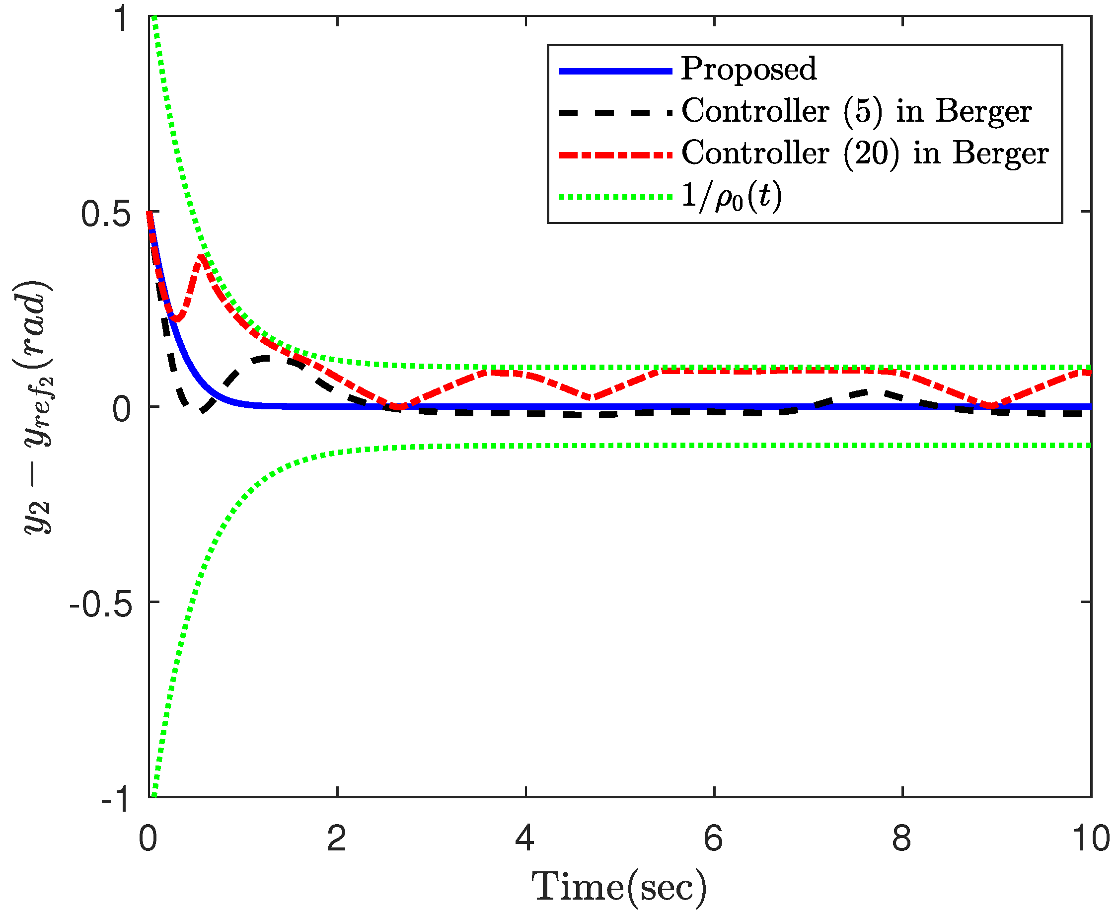
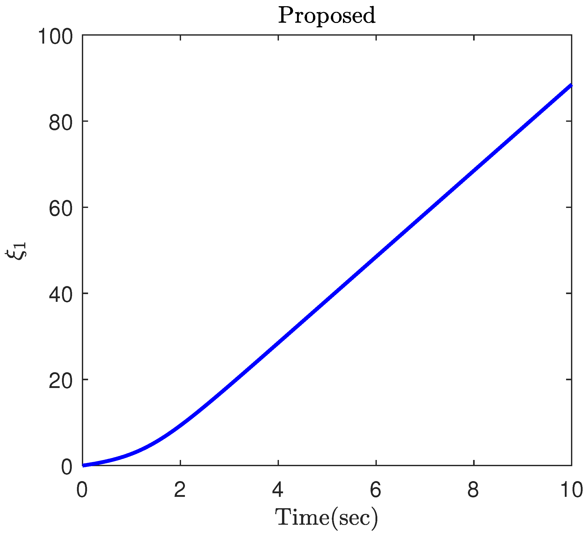
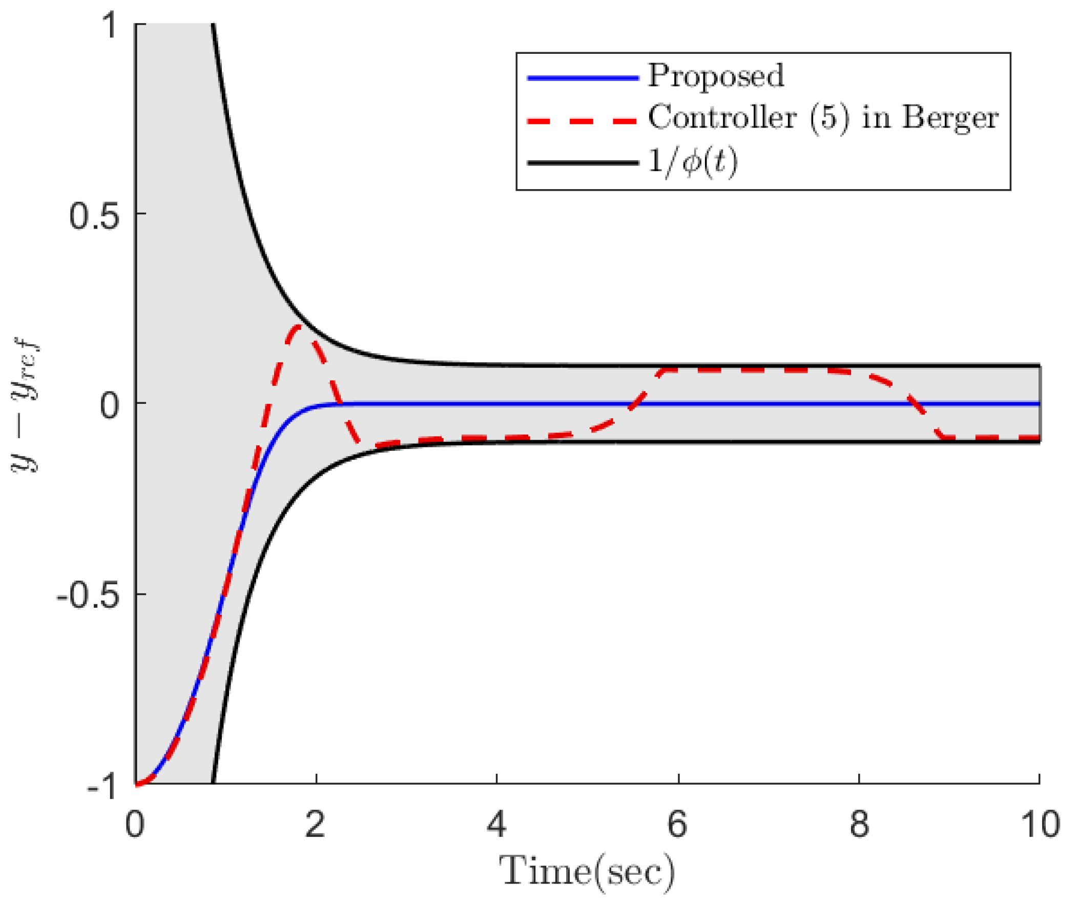
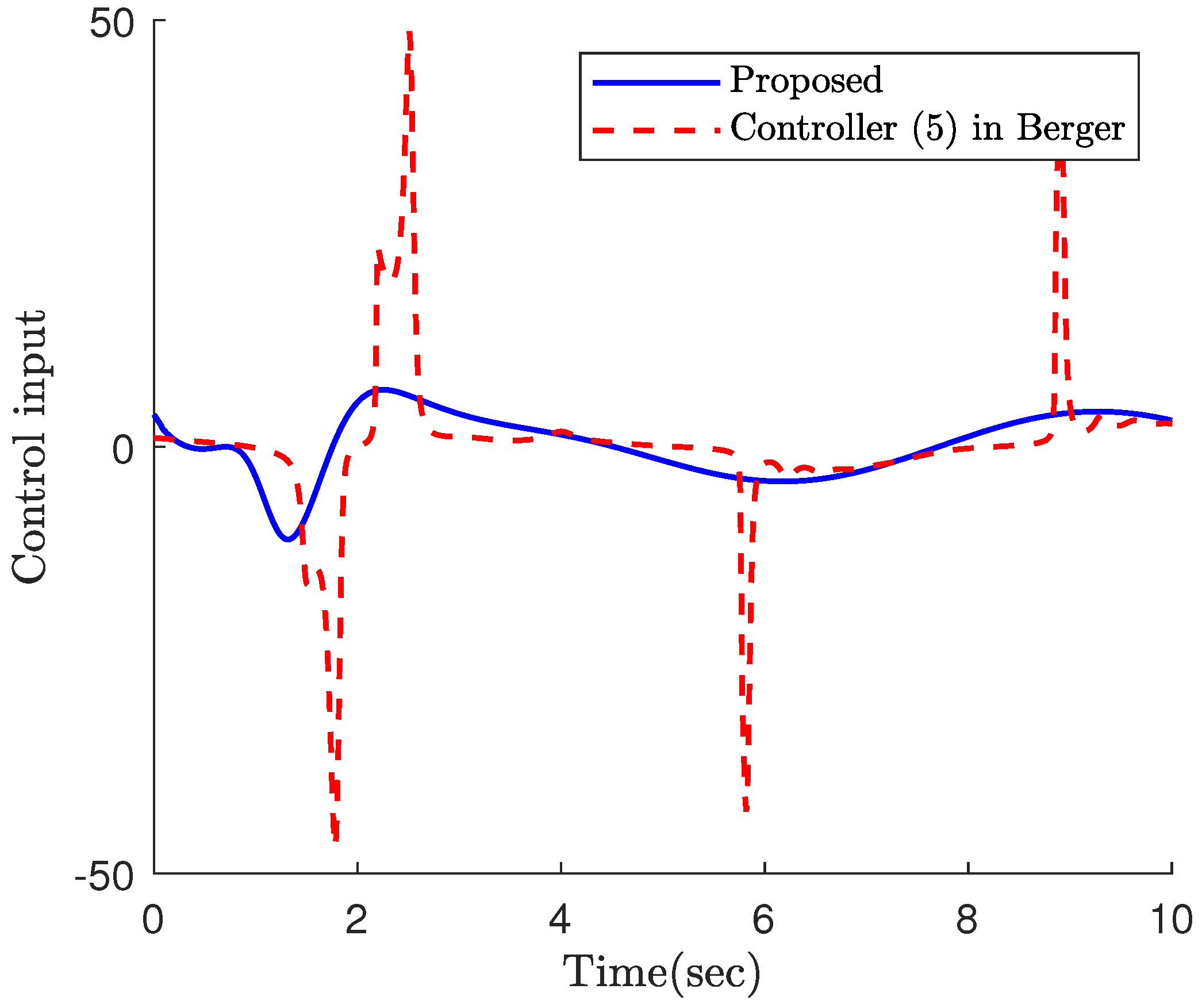
4. Simulation Results

To evaluate the efficacy of the suggested constrained control framework, the simulation results are provided in three parts.

Part 1: Firstly, a robotic manipulator illustrated in Figure 1 is taken into account [47]. This is a 2-DOF planar rigid robotic manipulator with revolute joints whose equations of motions are described by

$$\begin{array}{c}\hfill M\left(y\right)\ddot{y}+C(y,\dot{y})\dot{y}+G\left(y\right)=u,\end{array}$$

(25)

where the inertia matrix M, the centrifugal and Coriolis force matrix C, and the gravity vector G are, respectively, given by

$$\begin{array}{c}\hfill M=\left[\begin{array}{cc}{m}_1{l}_1^2+m_2(l_1^2+l_2^2+2l_1{l}_{2}cos\left(y_2\right))& m_2(l_2^2+l_1{l}_{2}cos\left(y_2\right))\\ m_2(l_2^2+l_1{l}_{2}cos\left(y_2\right))m2l_2^2& 0\end{array}\right],\end{array}$$

$$\begin{array}{c}\hfill C=\left[\begin{array}{cc}-2m_2{l}_1{l}_{2}sin\left(y_2\right)v_1& -m_2{l}_1{l}_{2}sin\left(y_2\right)v_2\\ -m_2{l}_1{l}_{2}sin\left(y_2\right)v_1& 0\end{array}\right],\end{array}$$

$$\begin{array}{c}\hfill G=g\left[\begin{array}{c}{m}_1{l}_{1}cos\left(y_1\right)+m_2(l_{1}cos\left(y_1\right)+l_{2}cos(y_1+y_2))\\ m_2{l}_{2}cos(y_1+y_2)\end{array}\right]\end{array}$$

where $m_1$ and $m_2$ denote the mass and $l_1$ and $l_2$ represent the length of the links, $g=9.81$ m/s² is the acceleration gravity, and $y_1$ and $y_2$ are the joint angles. The system parameters, the initial conditions and the reference trajectories are, respectively, taken as $m_1=m_2=1$ kg, $l_1=l_2=1$ m, $y\left(0\right)=\dot{y}\left(0\right)=0$, $y_{ref,1}\left(t\right)=sin\left(t\right)$, and $y_{ref,2}\left(t\right)=sin\left(2t\right)$. The parameters of the controller (12) along with the FTPPF (5) are chosen as $K_1=\mathrm{diag}\{2,2\}$, $K_2=\mathrm{diag}\{1,1\}$, $K_3=\mathrm{diag}\{1,1\}$, $K_4=\mathrm{diag}\{5,5\}$, ${\gamma }_1=0.9$, ${\gamma }_2=0.6$, $p_1=p_2=0.1$, $ϵ=0.002$, ${\rho }_0=1$, ${\rho }_T=0.01$, and $\kappa =0.5$. In this part, the simulation is repeated for different values of $T_f$ to investigate how this parameter affects the convergence property of the tracking errors. The simulation results are provided in Figure 2, Figure 3, Figure 4, Figure 5 and Figure 6. The time response of the tracking errors is illustrated in Figure 2 and Figure 3. Based on these two figures, it is clear that the proposed constrained control (12) is capable of satisfying the desired transient and steady state performances such as convergence rate and ultimate tracking error. Moreover, the proposed control is still able to meet the constraint on the tracking error even if the convergence time of the FTPPF is selected quite small. However, when the parameter $T_f$ is very small, then the controller is required to provide more control effort in order to maintain the error trajectory within its allowable region; otherwise, the error trajectory intercepts the boundary of the region and the constraint is violated. Therefore, from Figure 4 and Figure 5, the smaller convergence time is selected, the larger control effort is required. Moreover, parameter ${\xi }_1$ has been illustrated in Figure 6. Based on the definition of ${\xi }_1$, it is a positive and increasing function since it is the integral of a positive function. It should be pointed out although the value of ${\xi }_1$ becomes larger as time goes, it is multiplied by $x_2$, which very quickly converges to zero and has a small value.

Part 2: In this part, the objective is to compare the proposed constrained control (12) with the constrained controls (5) and (20) in Berger [47]. In fact, ref. [47] is a constrained control for nonlinear systems and is a suitable candidate to investigate the efficacy of the proposed constrained control framework. The simulation results of the three controllers applied to the robotic manipulator (25) are illustrated in Figure 7, Figure 8, Figure 9, Figure 10 and Figure 11. In fact, the main focus of the constrained controls (5) and (20) in Berger [47] is to satisfy constraints on the tracking error, and they are not able to make the tracking errors converge to zero. Based on this example, the proposed control accomplishes superior performance over the two controls in Berger [47]. More specifically, the error trajectory under the proposed control shows oscillation neither in the transient nor the steady state. Moreover, the proposed approach results in a faster and more accurate convergence. Despite the better performance of the proposed approach, it requires less control energy, which is of crucial importance practically. This fact can be clearly observed in Figure 9 and Figure 10. Similar to the previous part, the parameter ${\xi }_1$ is depicted in Figure 11, which confirms the theoretical results provided in this paper.

Part 3: Now, the suggested control, along with the constrained control (5) in Berger [47], is applied to a mass-spring system mounted on a car [47] illustrated in Figure 12. This system is described as follows. The mass $m_2$ is moving on a ramp that is inclined by the angle $\alpha$ and mounted on a car with mass $m_1$ for which the force F acts as the control input. The equation of motion for the aforementioned system can be expressed as

$$\begin{array}{c}\hfill \left[\begin{array}{cc}{m}_1+m_2& m_{2}cos\left(\alpha \right)\\ m_{2}cos\left(\alpha \right)& m_2\end{array}\right]\left[\begin{array}{c}\ddot{x}\left(t\right)\\ \ddot{s}\left(t\right)\end{array}\right]+\left[\begin{array}{c}0\\ ks\left(t\right)+d\dot{s}\left(t\right)\end{array}\right]=\left[\begin{array}{c}u\left(t\right)\\ 0\end{array}\right],\end{array}$$

(26)

in which the horizontal car position and the relative position of the mass on the ramp are denoted by x and s, respectively. The parameters k and d represent the coefficients of the spring and damper, respectively. The system output is defined as $y\left(t\right)=x\left(t\right)+s\left(t\right)cos\left(\alpha \right)$. It is supposed that a reference trajectory given by $y_{ref}\left(t\right)=cos\left(t\right)$ is going to be tracked by the system output. The initial condition is taken as $x\left(0\right)=s\left(0\right)=0$ and $\dot{x}\left(0\right)=\dot{s}\left(0\right)=0$. The parameters of the system (26) and the controller (12) are, respectively, $m_1=4$ kg, $m_2=1$ kg, $k=2$ N/m, $d=1$ Ns/m, $\alpha =\pi /4$ rad, $K_1=K_2=0.8$, $K_3=0.1$, $K_4=0.5$, ${\gamma }_1=0.9$, and ${\gamma }_2=0.8$,

From Figure 13, it is observed that both controllers are able to keep the error trajectory within the permitted region constructed by the performance function. However, the controller (5) in Berger could not provide convergence of the error trajectory to zero. As it is seen in this figure, the focus of this controller is to maintain the trajectory within the region and prevent any contact with the boundary. Nevertheless, the proposed control not only tries to satisfy the constraint, but it also drives the error trajectory to zero to provide perfect tracking. Based on Figure 14, although the proposed control results in a superior performance in a transient as well as a steady state, it requires less control energy. In this case, since the error trajectory does not approach the boundary, there is no sudden increase in the control input. Figure 15 illustrates the parameter $\xi$ of the proposed constrained control. It is worth mentioning that this figure confirms the importance of guaranteeing the convergence of the system state. In other words, if the system state is not decaying, the amplitude of the control input will be increasing since the parameter $\xi$ grows by time and it proportionally appears in the control input.

5. Conclusions

This study is concerned with the difficult issue of smooth, nonsingular, finite-time tracking control for EL systems with prescribed performance in spite of the system uncertainty and disturbance. It is rigorously proved that the closed-loop EL system is finite-time stable and that the singularity resulting from the use of fractional power can be successfully removed without having to construct a piecewise continuous function. In contrast to the existing constrained controls with complicated structures, the proposed control scheme accomplishes the desirable performance via introducing a time-varying gain in the sliding surface. The simulation results confirmed the effectiveness and usefulness of the new control framework.

References

1. Yu, S.; Yu, X.; Shirinzadeh, B.; Man, Z. Continuous finite-time control for robotic manipulators with terminal sliding mode. Automatica 2005, 41, 1957–1964. [Google Scholar] [CrossRef]
2. Lu, P.; Huang, W.; Xiao, J.; Zhou, F.; Hu, W. Adaptive Proportional Integral Robust Control of an Uncertain Robotic Manipulator Based on Deep Deterministic Policy Gradient. Mathematics 2021, 9, 2055. [Google Scholar] [CrossRef]
3. Gao, J.; Fu, Z.; Zhang, S. Adaptive fixed-time attitude tracking control for rigid spacecraft with actuator faults. IEEE Trans. Ind. Electron. 2018, 66, 7141–7149. [Google Scholar] [CrossRef]
4. Zakeri, E.; Farahat, S.; Moezi, S.A.; Zare, A. Robust sliding-mode control of a mini unmanned underwater vehicle equipped with a new arrangement of water jet propulsions: Simulation and experimental study. Appl. Ocean Res. 2016, 59, 521–542. [Google Scholar] [CrossRef]
5. Li, Y.; Zhao, D.; Zhang, Z.; Liu, J. An IDRA approach for modeling helicopter based on Lagrange dynamics. Appl. Math. Comput. 2015, 265, 733–747. [Google Scholar] [CrossRef]
6. Liang, C.D.; Ge, M.F.; Liu, Z.W.; Ling, G.; Zhao, X.W. A novel sliding surface design for predefined-time stabilization of Euler–Lagrange systems. Nonlinear Dyn. 2021, 106, 445–458. [Google Scholar] [CrossRef]
7. Shao, K.; Tang, R.; Xu, F.; Wang, X.; Zheng, J. Adaptive sliding-mode control for uncertain Euler–Lagrange systems with input saturation. J. Frankl. Inst. 2021, 358, 8356–8376. [Google Scholar] [CrossRef]
8. Deng, Q.; Peng, Y.; Han, T.; Qu, D. Event-triggered bipartite consensus in networked Euler–Lagrange systems with external disturbance. IEEE Trans. Circuits Syst. II Express Briefs 2021, 68, 2870–2874. [Google Scholar] [CrossRef]
9. Liu, H.; Gao, Z.; Cao, L.; Jiang, Z.; Zhang, J.; Song, Y. Tracking control of uncertain Euler–Lagrange systems with fading and saturating actuations: A low-cost neuroadaptive proportional-integral-derivative approach. Int. J. Robust Nonlinear Control 2022, 32, 2705–2721. [Google Scholar] [CrossRef]
10. Zhang, G.; Cheng, D. Adaptive fault-tolerant guaranteed performance control for Euler–Lagrange systems with its application to a 2-link robotic manipulator. IEEE Access 2020, 8, 184160–184171. [Google Scholar] [CrossRef]
11. Hu, Q.; Xiao, B.; Shi, P. Tracking control of uncertain Euler–Lagrange systems with finite-time convergence. Int. J. Robust Nonlinear Control 2015, 25, 3299–3315. [Google Scholar] [CrossRef]
12. Islam, S.; Liu, X.P. Robust sliding-mode control for robot manipulators. IEEE Trans. Ind. Electron. 2010, 58, 2444–2453. [Google Scholar] [CrossRef]
13. Pereira, A.R.; Hsu, L.; Ortega, R. Globally stable adaptive formation control of Euler–Lagrange agents via potential functions. In Proceedings of the 2009 American Control Conference, St. Louis, MO, USA, 10 July 2009; pp. 2606–2611. [Google Scholar]
14. Hong, Y.; Xu, Y.; Huang, J. Finite-time control for robot manipulators. Syst. Control Lett. 2002, 46, 243–253. [Google Scholar] [CrossRef]
15. Zhao, Y.; Duan, Z.; Wen, G. Distributed finite-time tracking of multiple Euler–Lagrange systems without velocity measurements. Int. J. Robust Nonlinear Control 2015, 25, 1688–1703. [Google Scholar] [CrossRef]
16. Hu, H.X.; Wen, G.; Yu, W.; Cao, J.; Huang, T. Finite-time coordination behavior of multiple Euler–Lagrange systems in cooperation-competition networks. IEEE Trans. Cybern. 2019, 49, 2967–2979. [Google Scholar] [CrossRef]
17. Huang, X.; Lin, W.; Yang, B. Global finite-time stabilization of a class of uncertain nonlinear systems. Automatica 2005, 41, 881–888. [Google Scholar] [CrossRef]
18. Nguyen, N.P.; Mung, N.X.; Thanh Ha, L.N.N.; Huynh, T.T.; Hong, S.K. Finite-time attitude fault tolerant control of quadcopter system via neural networks. Mathematics 2020, 8, 1541. [Google Scholar] [CrossRef]
19. Galicki, M. Finite-time control of robotic manipulators. Automatica 2015, 51, 49–54. [Google Scholar] [CrossRef]
20. Yao, Q.; Jahanshahi, H. Novel finite-time adaptive sliding mode tracking control for disturbed mechanical systems. Proc. Inst. Mech. Eng. Part C J. Mech. Eng. Sci. 2022, 236. [Google Scholar] [CrossRef]
21. Luan, F.; Na, J.; Huang, Y.; Gao, G. Adaptive neural network control for robotic manipulators with guaranteed finite-time convergence. Neurocomputing 2019, 337, 153–164. [Google Scholar] [CrossRef]
22. He, W.; Xu, C.; Han, Q.L.; Qian, F.; Lang, Z. Finite-Time L2 Leader–Follower Consensus of Networked Euler–Lagrange Systems With External Disturbances. IEEE Trans. Syst. Man, Cybern. Syst. 2017, 48, 1920–1928. [Google Scholar] [CrossRef]
23. Huang, B.; Zhang, S.; He, Y.; Wang, B.; Deng, Z. Finite-time anti-saturation control for Euler–Lagrange systems with actuator failures. ISA Trans. 2022, 124, 468–477. [Google Scholar] [CrossRef] [PubMed]
24. Li, R.; Yang, L.; Chen, Y.; Lai, G. Adaptive sliding-mode control of Robot Manipulators with System Failures. Mathematics 2022, 10, 339. [Google Scholar] [CrossRef]
25. Wang, D.; Liu, S.; He, Y.; Shen, J. Barrier Lyapunov function-based adaptive back-stepping control for electronic throttle control system. Mathematics 2021, 9, 326. [Google Scholar] [CrossRef]
26. Kim, J.H.; Yoo, S.J. Adaptive event-triggered control strategy for ensuring predefined three-dimensional tracking performance of uncertain nonlinear underactuated underwater vehicles. Mathematics 2021, 9, 137. [Google Scholar] [CrossRef]
27. He, W.; Huang, H.; Ge, S.S. Adaptive neural network control of a robotic manipulator with time-varying output constraints. IEEE Trans. Cybern. 2017, 47, 3136–3147. [Google Scholar] [CrossRef]
28. Cruz-Ortiz, D.; Chairez, I.; Poznyak, A. Non-singular terminal sliding-mode control for a manipulator robot using a barrier Lyapunov function. ISA Trans. 2022, 121, 268–283. [Google Scholar] [CrossRef]
29. Xia, J.; Zhang, Y.; Yang, C.; Wang, M.; Annamalai, A. An improved adaptive online neural control for robot manipulator systems using integral Barrier Lyapunov functions. Int. J. Syst. Sci. 2019, 50, 638–651. [Google Scholar] [CrossRef] [Green Version]
30. Chen, R.; Wang, Z.; Che, W. Adaptive Sliding Mode Attitude-Tracking Control of Spacecraft with Prescribed Time Performance. Mathematics 2022, 10, 401. [Google Scholar] [CrossRef]
31. Hua, C.; Chen, J.; Li, Y.; Li, L. Adaptive prescribed performance control of half-car active suspension system with unknown dead-zone input. Mech. Syst. Signal Process. 2018, 111, 135–148. [Google Scholar] [CrossRef]
32. Gao, S.; Liu, X.; Jing, Y.; Dimirovski, G.M. Finite-time prescribed performance control for spacecraft attitude tracking. IEEE/ASME Trans. Mechatron. 2021. [Google Scholar] [CrossRef]
33. Golestani, M.; Zhang, W.; Yang, Y.; Xuan-Mung, N. Disturbance observer-based constrained attitude control for flexible spacecraft. IEEE Trans. Aerosp. Electron. Syst. 2022. [Google Scholar] [CrossRef]
34. Dai, S.L.; He, S.; Ma, Y.; Yuan, C. Cooperative learning-based formation control of autonomous marine surface vessels with prescribed performance. IEEE Trans. Syst. Man, Cybern. Syst. 2022, 52, 2565–2577. [Google Scholar] [CrossRef]
35. Huang, S.; Wang, J.; Xiong, L.; Liu, J.; Li, P.; Wang, Z. Distributed Predefined-Time Fractional-Order sliding-mode control for Power System With Prescribed Tracking Performance. IEEE Trans. Power Syst. 2022, 37, 2233–2246. [Google Scholar] [CrossRef]
36. Zhang, J.X.; Yang, G.H. Fault-tolerant output-constrained control of unknown Euler–Lagrange systems with prescribed tracking accuracy. Automatica 2020, 111, 108606. [Google Scholar] [CrossRef]
37. Yin, Z.; Luo, J.; Wei, C. Robust prescribed performance control for Euler–Lagrange systems with practically finite-time stability. Eur. J. Control 2020, 52, 1–10. [Google Scholar] [CrossRef]
38. Wang, M.; Yang, A. Dynamic learning from adaptive neural control of robot manipulators with prescribed performance. IEEE Trans. Syst. Man, Cybern. Syst. 2017, 47, 2244–2255. [Google Scholar] [CrossRef]
39. Yao, Q. Robust adaptive finite-time prescribed performance attitude tracking control of spacecraft. Int. J. Aeronaut. Space Sci. 2021, 22, 1183–1193. [Google Scholar] [CrossRef]
40. Jing, C.; Xu, H.; Niu, X. Adaptive sliding mode disturbance rejection control with prescribed performance for robotic manipulators. ISA Trans. 2019, 91, 41–51. [Google Scholar] [CrossRef]
41. Lyu, W.; Zhai, D.H.; Xiong, Y.; Xia, Y. Predefined performance adaptive control of robotic manipulators with dynamic uncertainties and input saturation constraints. J. Frankl. Inst. 2021, 358, 7142–7169. [Google Scholar] [CrossRef]
42. Liu, H.; Tian, X.; Wang, G.; Zhang, T. Finite-time H control for high-precision tracking in robotic manipulators using backstepping control. IEEE Trans. Ind. Electron. 2016, 63, 5501–5513. [Google Scholar] [CrossRef]
43. Song, Z.; Duan, C.; Wang, J.; Wu, Q. Chattering-free full-order recursive sliding-mode control for finite-time attitude synchronization of rigid spacecraft. J. Frankl. Inst. 2019, 356, 998–1020. [Google Scholar] [CrossRef]
44. Yu, J.; Shi, P.; Zhao, L. Finite-time command filtered backstepping control for a class of nonlinear systems. Automatica 2018, 92, 173–180. [Google Scholar] [CrossRef]
45. Golestani, M.; Esmailzadeh, M.; Mobayen, S. Constrained attitude control for flexible spacecraft: Attitude pointing accuracy and pointing stability improvement. IEEE Trans. Syst. Man, Cybern. Syst. 2022. [Google Scholar] [CrossRef]
46. Cao, L.; Xiao, B.; Golestani, M. Robust fixed-time attitude stabilization control of flexible spacecraft with actuator uncertainty. Nonlinear Dyn. 2020, 100, 2505–2519. [Google Scholar] [CrossRef]
47. Berger, T.; Lê, H.H.; Reis, T. Funnel control for nonlinear systems with known strict relative degree. Automatica 2018, 87, 345–357. [Google Scholar] [CrossRef]
Figure 1. Planar rigid revolute joint robotic manipulator.
Mathematics 10 03850 g001
Figure 2. The tracking error of the first joint under different T f .
Mathematics 10 03850 g002
Figure 3. The tracking error of the second joint under different T f .
Mathematics 10 03850 g003
Figure 4. The first component of the control input.
Mathematics 10 03850 g004
Figure 5. The second component of the control input.
Mathematics 10 03850 g005
Figure 6. The parameter ξ 1 under different T f .
Mathematics 10 03850 g006
Figure 7. The tracking error of the first joint in Part 2.
Mathematics 10 03850 g007
Figure 8. The tracking error of the second joint in Part 2.
Mathematics 10 03850 g008
Figure 9. The first component of the control input in Part 2.
Mathematics 10 03850 g009
Figure 10. The second component of the control input in Part 2.
Mathematics 10 03850 g010
Figure 11. The parameter ξ 1 in Part 2.
Mathematics 10 03850 g011
Figure 12. Mass on car system.
Mathematics 10 03850 g012
Figure 13. The tracking error in Part 3.
Mathematics 10 03850 g013
Figure 14. The control input in Part 3.
Mathematics 10 03850 g014
Figure 15. The parameter ξ 1 in Part 3.
Mathematics 10 03850 g015
Publisher’s Note: MDPI stays neutral with regard to jurisdictional claims in published maps and institutional affiliations.