Nonlinear Frequency-Modulated Waveforms Modeling and Optimization for Radar Applications

Abstract

Conventional radars commonly use a linear frequency-modulated (LFM) waveform as the transmitted signal. The LFM radar is a simple system, but its impulse-response function produces a −13.25 dB sidelobe, which in turn can make the detection of weak targets difficult by drowning out adjacent weak target information with the sidelobe of a strong target. To overcome this challenge, this paper presents a modeling and optimization method for non-linear frequency-modulated (NLFM) waveforms. Firstly, the time-frequency relationship model of the NLFM signal was combined by using the Legendre polynomial. Next, the signal was optimized by using a bio-inspired method, known as the Firefly algorithm. Finally, the numerical results show that the advantages of the proposed NLFM waveform include high resolution and high sensitivity, as well as ultra-low sidelobes without the loss of the signal-to-noise ratio (SNR). To the authors’ knowledge, this is the first study to use NLFM signals for target-velocity improvement measurements. Importantly, the results show that mitigating the sidelobe of the radar waveform can significantly improve the accuracy of the velocity measurements.

1. Introduction

The linear frequency-modulated (LFM) waveform is widely used in radar systems, such as the synthetic aperture radar [1], the millimetre wave radar [2,3], and the weather radar [4]. The linear time-frequency relationship of the LFM signal allows the output signal from the mixing receiver to be a low-pass signal that does not require complex matching-filter operations to produce pulse-compressed signal-processing gains, thus making the radar system simple and achieving low complexity in terms of its signal processing operations. In addition, the LFM signal is easily generated using a voltage-controlled oscillator, which allows for flexible settings of the signal period and tuning-frequency parameters.

However, the impulse-response function (IRF) of the LFM radar has a peak sidelobe ratio (PSLR) of −13.25 dB [5]. Under the influence of this signal sidelobe, the sidelobe energy of the signal from a strong target may be higher than the mainlobe energy of the weak target, which in turn leads to the neighbouring weak targets being swamped by the sidelobe of the strong target. In fact, some weak targets are indeed high-value targets for radar detection, such as pedestrians and birds.

As a result, many scholars have attempted to reduce the sidelobe of radar IRF by fundamentally designing the different waveforms. In recent years, attention has been paid to non-linear frequency-modulated (NLFM) waveforms, which have a non-linear time-frequency relationship and offer flexible signal design freedom [6,7]. Wang et al. [8] demonstrateed the airborne synthetic aperture radar experiment using an NLFM waveform. In the underlying experiment, the construction of the NLFM signal is investigated, showing the merits of the NLFM. In our previous work [9], the spectral density distribution function of the NLFM waveform was defined by using an optimized Kaiser function, and the phases of the NLFM waveform were formulated as a problem of phase retrieval. Thanks to nonuniqueness solutions, the proposed NLFM waveform generates the orthogonal signals with a good random phase diversity. Subsequently, orthogonal NLFM signals were presented to reduce the sidelobe effect of the impulse-response function of the point target, and the interference arising from neighboring radars [10]. Xu et al. [11] investigated the opportunity of designing the transmitted signals using the orthogonal NLFM waveform and demonstrated that NLFM signals outperform conventional the LFM signal. In [12], the NLFM waveform was applied to the multiple-input and multiple-output radar.

Unlike the above-mentioned methods, this paper presents a modeling and optimization method for NLFM waveforms by using the Legendre polynomial. The optimized NLFM signal was explored using the Firefly algorithm [13]. Furthermore, to the best of our knowledge, this is the first study to investigate how the sidelobe of IRF affects radar target velocity measurements. The remainder of this paper is outlined below. Section 2 presents the modeling and optimization approach of the proposed NLFM. Section 3 shows the numerical results of the optimized NLFM, which clearly distinguishes pedestrians from vehicles without the loss of the signal-to-noise ratio (SNR). Finally, Section 4 draws conclusions.

2. Modeling and Optimization of NLFM Waveform

2.1. Modeling of NLFM Waveforms

The time-frequency (TF) functions of the NLFM signals are modeled as

$$\mathrm{TF}\left(t\right)=\sum _{n=1}^N{a}_n{P}_{2n-1}\left(2t\right), -0.5<t<0.5,$$

(1)

where t is time, $P_n\left(t\right)$ is the n-th degree Legendre Polynomials (LPs) at t, N is the order of LPs, and $a_n$ is the coefficient of the polynomials.

For simplicity, the coefficients $a_n,1\le n\le N$ are denoted as a vector $\mathbf{a}$. To ensure that the waveform is symmetry [14], the degree of the LPs is set to be odd. Here, we use the LPs of odd degrees 1 through 9 to formulate the TF functions of the NLFM signal.

Figure 1 shows these LPs with odd degrees. For the conventional linear frequency-modulated (LFM) signal, the coefficients of the higher order of LPs are equivalent to zero. Integrating the TF functions of (1), the phase of the NLFM signal can be obtained as

$$\phi \left(t\right)=2\pi {\int }_{-0.5}^{0.5}\sum _{n=1}^5{a}_n{P}_{2n-1}\left(2t\right)dt,-0.5<t<0.5.$$

(2)

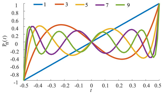
Figure 1. Legendre polynomials of odd degrees 1 through 9.

Finally, the NLFM signal with an amplitude A is completely specified as

$$s\left(t\right)=e^{j(2\pi f_{0}t+\phi \left(t\right))}=e^{j2\pi (f_{0}t+{\int }_{-0.5}^{0.5}{\sum }_{n=1}^5{a}_n{P}_{2n-1}\left(2t\right)dt)},$$

(3)

where $f_0$ is the center frequency of the NLFM signal.

As shown in Figure 2, the NLFM signal waveform is modeled as follows:

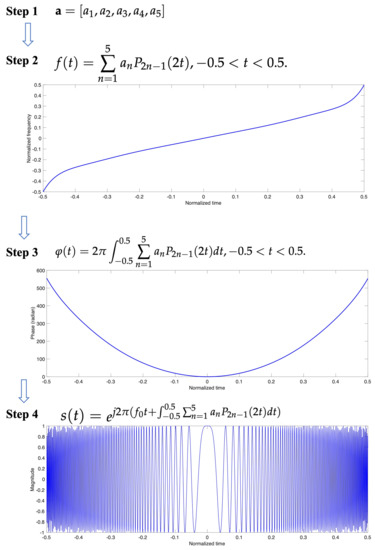
Figure 2. Procedures for modelling NLFM waveforms.

Step 1:

Input the coefficient vector of the Legendre polynomial $\mathbf{a}=[a_1,a_2,a_3,a_4,a_5]$;

Step 2:

Define a frequency function of time based on the coefficient vector of the Legendre polynomial using Equation (1);

Step 3:

Integrate the frequency function to obtain the phase function using Equation (2);

Step 4:

Output the NLFM signal waveform using Equation (3);

Step 5:

Assess the signal performance.

Typically, three metrics are used to assess the performance of the IRF for NLFM signals [1]: the factor of mainlobe width broadening (MW), the peak sidelobe ration (PSLR), and the integreated side-lobe ration (ISLR). Using the same bandwidth and the period of the LFM signal as a reference, the MW of IRF for NLFM signals is typically 3 dB below the highest energy point. To better evaluate the mainlobe width, the width of the zero point on both sides of the highest energy point is used for calculating MW (null-to-null width), as plotted in Figure 3. The PSLR is the ratio of the maximum sidelobe to the peak. The ISLR is the power ratio of the integrated sidelobe to the mainlobe. In general, an ideal PSLR performance corresponds to better ISLR, so only the PSLR is used as the measurement metric in this paper.

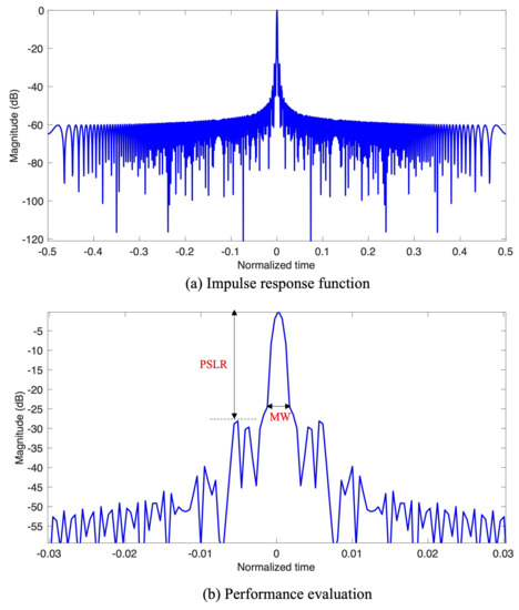
Figure 3. Signal performance evaluation.

The results of modeling the NLFM signal with four coefficient vectors of LPs and their performance are shown in Figure 4, where the left column shows the time-frequency relationship of the signal and the right column shows the corresponding IRFs. These four sets of LP coefficient vectors a are [1 1 1 1 1], [1 1 2 1 −1], [1 1 3 1 1], and [0.2 1 3 2 1]. As can be seen from the numerical results, small differences in the coefficients produce widely varying time-frequency functions as well as different performance IRFs.

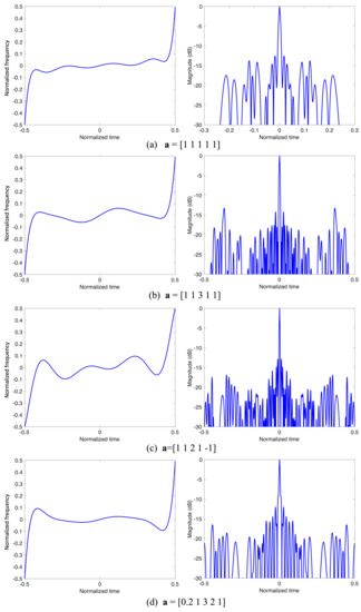
Figure 4. Modeling the NLFM signal with four coefficient vectors of LPs. The plots in the left column show the time-frequency relationship of the signal, and the right column shows the corresponding IRFs.

In summary, it can be seen that the above formulations generate good diversity for the NLFM waveform. Consequently, the next stage is performed to explore the optimal waveform.

2.2. Optimization of NLFM Waveform

A better NLFM waveform depends on a relatively narrower MW and a lower PSLR. Unfortunately, the lower levels of sidelobes are achieved at the cost of a broadening of the main-lobe width that governs the resolution of the underlying system. Hence, the PSLR and the MW were used to formulate an optimization fitness function under the vector coefficients $\mathbf{a}=\{a_n,1\le n\le 5\}$

$$\mathrm{Fitness}\left(\mathbf{a}\right)=\mathrm{PSLR}\left(\mathbf{a}\right)-\lambda (\mathrm{MW}\left(\mathbf{a}\right)-1.6),\mathbf{a}\in {\Re }^N,$$

(4)

where $\lambda$ is is a penalty factor to adjust the broadening factor of the MW, the MW refers to the MW of the IRF of the LFM, and the constant value of 1.6 keeps the broadening factor of MW to no more than 1.6.

One bio-inspired method, the firefly algorithm (FA), is applied to explore the optimal coefficients because the algorithmic structure of FA used in this paper is highly similar to the structure of algorithm in [13,15].

The main steps of FA are the updating of the light intensity, the ranking of the fireflies, and the movement of the fireflies. Here, one firefly represents one coefficient vector of LPs. The brightness I of a firefly at a particular location p is chosen as

$$I\left(\mathbf{a}\right)=\mathrm{Fitness}\left(\mathbf{a}\right).$$

(5)

It decreases with distance r via $e^{-\gamma r^2}$, where $\gamma$ is a parameter characterizing the variation of the brightness.

The attractiveness of a firefly is proportional to the light intensity observed by adjacent fireflies. It is defined as

$$\rho ={\rho }_0{e}^{-\gamma r^2},$$

(6)

where ${\rho }_0$ is the attractiveness at $r=0$. The distance between any two fireflies k and l at ${\mathbf{a}}_k$ and ${\mathbf{a}}_l$ is measured by the Cartesian distance as

$$r_{kl}=\sqrt{\sum _{i=1}^5{a}_k\left(i\right)-a_l\left(i\right)},$$

(7)

The movement of the fireflies is defined as follows:

$$a_k\left(i\right)=a_k\left(i\right)+{\rho }_0{e}^{-\gamma r^2}[a_k\left(i\right)-a_l\left(i\right)]+\alpha (\mathrm{rand}-0.5),$$

(8)

where $\alpha$ is the randomization parameter; it governs the rate of random movement for the fireflies, and $\mathrm{rand}$ is a Gaussian random number generator with zero mean and variance of one.

Based on the above discussion, the FA steps for NLFM optimization can be summarized as follows:

Step 1:

Initialize each firefly $\mathbf{a}$ as $a\left(i\right)=1+\mathrm{rand},1\le i\le 5.$

Step 2:

Modeling the NLFM waveforms using Equations (1)–(3), calculate the IRFs for all fireflies. Then, compute the MW and PSLR, and update the light intensity by Equation (4).

Step 3:

Rank the fireflies by light intensity and find the current global best solution (corresponding to the brightest one).

Step 4:

Move all fireflies toward the brighter ones by Equation (8).

Step 5:

Repeat Steps 2–5 until the iteration times reach the threshold of the objective function.

3. Numerical Results

The proposed approach is evaluated in terms of the following two aspects:

(1) The numerical results of the optimized NLFM signal;

(2) The advantages of the proposed NLFM for radar-target range and velocity measurements.

3.1. Numerical Results of the NLFM Signal

After performing the FA, the optimized coefficients have been explored. Hence, the optimized NLFM signal with any large time-bandwidth product can be specified using the optimized coefficients.

Here, the pulse width and the bandwidth of signal are set as 1.7 μs and 600 MHz, respectively, as an experimental study. It is thought that the oversampling factor is usually chosen to be between 1.1 and 1.4, to obtain efficient use of the data samples while maintaining an adequate gap in the spectrum [16]. Consequently, the oversampling factor is set as 1.2. Hence, the sampling rate is chosen as 720 MHz for the signals. Figure 5 shows the numerical results of the optimized NLFM signals. Because the LFM signals are commonly used in the PD radar, we use the LFM signal for comparison with the optimized NLFM signal. Figure 5a demonstrates the time frequency of the signals. Figure 5b plots the waveforms in the time domain. The IRF of both the LFM and NLFM signals is shown in the Figure 5c,d. Optimized by using the FA, the tradeoff between the MW and the PSLR is optimal for the optimized NLFM signal. The PSLR of the IRF of NLFM is −34.45 dB. The broadening factor of the MW of NLFM is 1.5, referring to that of the LFM signal. Although the PSLR of the IRF of the LFM signal can be achieved to −34.45 dB by applying windowed processing, it leads to a 1.12 dB SNR loss.

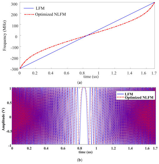
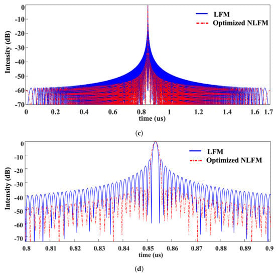
Figure 5. Comparisons of the optimized NLFM signal and the LFM signal: (a) time-frequency function, (b) waveforms, (c) IRF, and (d) zoom in the IRF.

3.2. Application of the Optimized NLFM Signal for Radar-Target Range and Velocity Measurements

We take the 77 GHz carrier wave as an example for the proposed NLFM waveform for radar applications. The optimized NLFM waveform is used as the transmitted signal. Taking the broadening factor of the MW into consideration, the range resolution is 0.375 m. The pulse-repeat frequency is 20 kHz, resulting in the maximum unambiguous velocity $v_{max}$ = 62.5 m/s and the maximum unambiguous range $R_{max}$ = 7.5 km. The coherent processing interval is chosen as 16 pulses. A typical road environment is illustrated in Figure 6, where a car and a pedestrian are in the scenario. The car target is located at 50.7 m in the range, moving forward at 10 m/s. The pedestrian is located at 50 m in the range, running in the opposite direction at 2 m/s. The radar cross section (RCS) is set as 0.3 for the pedestrian and 1 for the car, respectively.

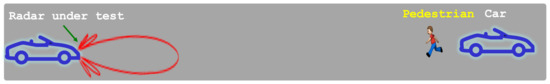
Figure 6. A representative scenario designed for experiment.

The proposed radar is compared with other related approaches, including the LFM radar, and the LFM radar using a windowed processing [16], denoted as WLFM for simplicity. The WLFM uses a Kaiser window with an adjustable parameter $\beta$ [16]. The $\beta$ is set as 4.4, generating a PSLR of −34.45dB. Using the different radars, the raw data are simulated at the different SNRs, shown in Figure 7. To show the plots clearly, the focused targets are analyzed by upsampling by a factor of eight. The range and velocity of the targets are processed and shown in Figure 8, at the SNR of 0 dB. Firstly, Figure 8 obviously shows that the information of the pedestrian is masked by the sidelobes in the case of the LFM radar. Hence, it is difficult to discriminate the pedestrian from the sidelobes of the car. Moreover, Figure 8a demonstrates a large error of the velocity of the pedestrian by the LFM radar, due to the high level of the sidelobes. The results of WLFM suggest that the effects of the sidelobe can be significantly reduced by using the windowed processing. However, the intensities of the targets have also decreased radically. This processing leads to a 1.12 dB of SNR loss. Interestingly, the proposed NLFM radar shows the best detection performance. Because the sidelobes are substantially reduced without any loss of SNR, the accuracy of the velocity measurements is also improved significantly. Above all, it can be found that the sidelobes highly decrease the accuracy of the velocity measurements. Furthermore, Table 1 summarizes how the high sidelobes affect the velocity measurements of the low RCS targets. We use the root mean square error (RMSE) to assess the measurements’ accuracy. The best results are highlighted in bold.

Figure 7. Raw data at different SNRs. (a) 30 dB. (b) 15 dB, and (c) 0 dB, respectively.

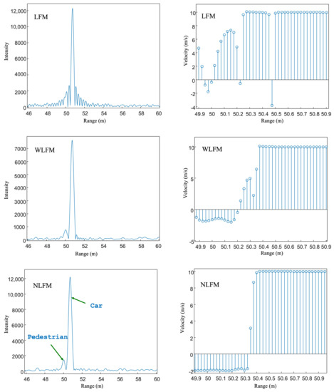
Figure 8. Range detection and velocity measurements for the targets at SNR of 0 dB.

Table 1. The RMSE of the pedestrian velocity (m/s).

SNR (dB)	LFM	WLFM	NLFM
0	7.302	1.441	0.665
15	7.254	1.378	0.641
30	7.249	1.365	0.630

Again, the proposed NLFM radar exhibits the most robust performance for measuring the low RCS targets under the interferences of high sidelobes. In practice, the detection of pedestrian is very important in improving the safety of pedestrian and traffic. However, the pedestrians are of low RCS targets and are usually around vehicular targets with high RCS. The above representative experiment demonstrates the advantages of the proposed NLFM radar.

4. Conclusions

High sensitivity and low sidelobes are of great importance to reliably detect the larger contrast targets, such as pedestrians and cars. The conventional LFM radars suffer from a PSLR of −13.25 dB. In this paper, a novel NLFM is modeled and optimized for radar sensing in high resolution and high sensitivity. The proposed NLFM signal has been modeled by using the Legendre polynomials and been optimized by using the FA. Compared with LFM and WLFM, the proposed NLFM shows the best performance on the sidelobe reduction, the SNR preservation, and the target range and velocity measurements. Interestingly, our findings reveal that the sidelobes significantly decrease the accuracy of the velocity measurements of the nearby target. The potential of the proposed approach offers lower power and highly reliable detection performance. In conclusion, the optimized NLFM shows promise for radar applications. Future work will implement the proposed NLFM signal on radar hardware to examine the performance of the signal in real-world radar applications.

References

- Curlander, J.C.; McDonough, R.N. Synthetic Aperture Radar Systems and Signal processing; Wiley: New York, NY, USA, 1991. [Google Scholar]
- Xu, Z.H.; Baker, C.J.; Pooni, S. Range and Doppler Cell Migration in Wideband Automotive Radar. IEEE Trans. Veh. Technol. 2019, 68, 5527–5536. [Google Scholar] [CrossRef]
- Xu, Z.; Xue, S.; Wang, Y. Incoherent Interference Detection and Mitigation for Millimeter-Wave FMCW Radars. Remote Sens. 2022, 14, 4817. [Google Scholar] [CrossRef]
- Kurdzo, J.M.; Cheong, B.L.; Palmer, R.D.; Zhang, G.; Meier, J.B. A pulse compression waveform for improved-sensitivity weather radar observations. J. Atmos. Ocean. Technol. 2014, 31, 2713–2731. [Google Scholar] [CrossRef][Green Version]
- Richards, M.A. Fundamentals of Radar Signal Processing; McGraw-Hill Education: New York, NY, USA, 2014. [Google Scholar]
- Milczarek, H.; Leśnik, C.; Djurović, I.; Kawalec, A. Estimating the Instantaneous Frequency of Linear and Nonlinear Frequency Modulated Radar Signals—A Comparative Study. Sensors 2021, 21, 2840. [Google Scholar] [CrossRef] [PubMed]
- Jin, G.; Deng, Y.; Wang, R.; Wang, W.; Wang, P.; Long, Y.; Zhang, Z.M.; Zhang, Y. An advanced nonlinear frequency modulation waveform for radar imaging with low sidelobe. IEEE Trans. Geosci. Remote Sens. 2019, 57, 6155–6168. [Google Scholar] [CrossRef]
- Wang, W.; Wang, R.; Zhang, Z.; Deng, Y.; Li, N.; Hou, L.; Xu, Z. First demonstration of airborne SAR with nonlinear FM chirp waveforms. IEEE Geosci. Remote Sens. Lett. 2016, 13, 247–251. [Google Scholar] [CrossRef]
- Xu, Z.H.; Shi, Q. Interference Mitigation for Automotive Radar Using Orthogonal Noise Waveforms. IEEE Geosci. Remote Sens. Lett. 2018, 15, 137–141. [Google Scholar] [CrossRef]
- Xu, Z.H.; Shi, Q.; Sun, L. Novel Orthogonal Random Phase-Coded Pulsed Radar for Automotive Application. J. Radars 2018, 7, 364–375. [Google Scholar] [CrossRef]
- Xu, Z.H.; Wang, R.; Ye, K.; Wang, W.; Quan, S.; Wei, M. Simultaneous range ambiguity mitigation and sidelobe reduction using orthogonal non-linear frequency-modulated (ONLFM) signals for satellite SAR Imaging. Remote Sens. Lett. 2018, 9, 829–838. [Google Scholar] [CrossRef]
- Zhao, Y.; Ritchie, M.; Lu, X.; Su, W.; Gu, H. Non-continuous piecewise nonlinear frequency modulation pulse with variable sub-pulse duration in a MIMO SAR radar system. Remote Sens. Lett. 2020, 11, 283–292. [Google Scholar] [CrossRef]
- Xu, Z.H.; Deng, Y.k.; Wang, Y. A novel optimization framework for classic windows using bio-inspired methodology. Circuits Syst. Signal Process. 2016, 35, 693–703. [Google Scholar] [CrossRef]
- Levanon, N.; Mozeson, E. Radar Signals; John Wiley & Sons: Hoboken, NJ, USA, 2004. [Google Scholar]
- Xu, Z.; Li, H.C.; Shi, Q.; Wang, H.; Wei, M.; Shi, J.; Shao, Y. Effect analysis and spectral weighting optimization of sidelobe reduction on SAR image understanding. IEEE J. Sel. Top. Appl. Earth Obs. Remote Sens. 2019, 12, 3434–3444. [Google Scholar] [CrossRef]
- Cumming, I.G.; Wong, F.H. Digital Processing of Synthetic Aperture Radar Data; Artech House: Norwood, MA, USA, 2005. [Google Scholar]
Publisher’s Note: MDPI stays neutral with regard to jurisdictional claims in published maps and institutional affiliations. |
© 2022 by the authors. Licensee MDPI, Basel, Switzerland. This article is an open access article distributed under the terms and conditions of the Creative Commons Attribution (CC BY) license (https://creativecommons.org/licenses/by/4.0/).