Abstract
In this paper, a new test statistic based on the weighted Frobenius norm of covariance matrices is proposed to test the homogeneity of multi-group population covariance matrices. The asymptotic distributions of the proposed test under the null and the alternative hypotheses are derived, respectively. Simulation results show that the proposed test procedure tends to outperform some existing test procedures.
Keywords:
high-dimensional data; weighted Frobenius norm; homogeneity test; martingale central limit theorem; asymptotic distributions MSC:
62H15; 62E20
1. Introduction
In the last thirty years, statistical methods have made great developments for high-dimensional data. One common feature of high-dimensional data is that the data dimension is larger or vastly larger than the total sample size. In high-dimensional settings, many classic methods are not well-defined or have poor performances. As a result, a great deal of statistical methods have been proposed to deal with high-dimensional data. As an important issue of statistical inference, hypothesis testing is being followed with interest by scholars. Testing the equality of several covariance matrices is a fundamental problem in multivariate statistical analysis and can be found in many relevant works, such as [1,2]. This problem will arise from the analysis of gene expression data. It was shown in [3] that many genes have different variances in gene expressions between disease states. For example, the dataset of the breast cancer of patient is classified in three groups based on their gene expression signatures: well-differentiated tumors, moderately differentiated tumors, and poorly differentiated and undifferentiated tumors. Refs. [4,5,6] respectively used artificial neural networks, feature selection and a Markov blanket-embedded genetic algorithm to investigate this dataset. This dataset includes 83 samples, which is greatly less than data dimension 2308. For this gene dataset, we are interested in checking whether the covariance matrices of the four groups are the same or not. It is noted that an important assumption for multivariate analysis of variance is that of equal covariance matrices in different groups. Therefore, testing the equality of several covariance matrices is needed. Specifically, assume are independent and identically distributed (iid) with a p-dimensional distribution with mean vector and covariance matrix for with . We want to test the following hypothesis
A classical method is the likelihood ratio test proposed by [7], where the population distribution is normal. However, as the data dimension is larger or vastly larger than the sample size, the likelihood ratio test is not well-defined because of the singularity of sample covariance matrices in probability one. Thus, it is vital to propose new procedures suitable to high-dimensional data. Owing to the curse of dimensionality, it becomes more challenging in high dimensions. For the hypothesis (1), there exists some test procedures in the literature. Based on the Frobenius norm, Refs. [8,9,10,11] proposed test statistics, respectively. Ref. [12] presented a test for high-dimensional longitudinal data. Ref. [13] proposed a power-enhancement high-dimensional test when the maximum eigenvalue of is bounded or for . Ref. [14] presented a test based on the well-known Box’s test ([15]) for high-dimensional normal data. It is noted that [9] imposed the conditions for to obtain the asymptotical null distribution of his test under normality, where is equal to the covariance matrix under the null hypothesis . Under high-dimensional normal data, [10] proposed a test as for . Ref. [8] imposed and other conditions to build asymptotical properties of his test statistic. The test statistics in [8,9,10,13,14] imposed the condition about the relationship between the data dimension p and the sample size or about the normal data. These conditions restrict the application of their test procedures. Ref. [11] gave a Frobenius norm-based test, which can be seen as an extension of that in [16], where the data dimension and the sample size can change arbitrarily.
The existing Frobenius norm-based tests for the hypothesis were almost constructed by , where means average covariance matrix of the population covariance matrices . The deviations of from overall is weighted by all equal weight , which, however, cannot emphasize the deviations of populations with large sample sizes. Based on this, we here construct a new test statistic by a different Frobenius norm where and . Here, is a weighted average of k covariance matrices, which can emphasize the deviations of populations with large sample sizes. On the other hand, it is evident that the null hypothesis holds if and only if .
The main purpose of this paper is to develop a new method to test the homogeneity of k high-dimensional covariance matrices on the basis of the weighted Frobenius norm. For the hypothesis in (1), most existing methods ([8,9,10,13]) imposed normality or the explicit relationship of between the data dimension p and the sample size n, and may behave poorly under non-normal data or ultra-high dimensional data. However, our method does not require normality or an explicit relationship between p and n, which is similar with the method in [11]. Thus, our method can be applied to non-normal and ultra-high dimensional data. On the other hand, the difference of the method in [11] and ours is that we use a sample-sizes-based Frobenius norm to build test statistics so that the tests in this paper and [11] behave differently, as the sample sizes are unequal. When , our proposed test statistic can be seen as an extension of that [16] except a constant. Hence it can also be applied to two-sample data.
Simulation results show that the proposed test behaves differently from existing tests such as the tests in [11,13,14]. We will discuss the differences between the proposed test and the competing tests through numerical comparisons in various scenarios. We observe that the proposed test outperforms the competing tests in both size and power in many cases.
The remainder of the paper is organized as follows. Section 2 first presents the statistical model and the imposed conditions in order to construct our new test. In Section 3, a new test statistic is proposed and its asymptotic properties are also given. Section 4 presents a numerical study of the proposed test to compare three competing tests. Concluding remarks are provided in Section 5. The proofs of main results are arranged in Appendix A.
2. Preliminaries
We consider the following general multivariate model that is often used in literature:
for and , where is a matrix for some such that and are r-variate iid random vectors with and . Furthermore, denote and have a finite eighth moment with where is some constant. Moreover, for any positive integers q and , there has
as , where are distinct indices. It shows from (2) that are pseudo-independent, which is naturally satisfied when samples are generated from normal distribution.
In order to obtain the asymptotic distributions of new test statistic, some conditions are imposed as follows:
- (C1)
- As , for .
- (C2)
- As , and for arbitrary , and .
(C1) implies that all sample sizes have the same increasing rate, except constant terms. (C2) can be seen as an extension of the condition A2 in [16] to the case of multi-groups. The two conditions are the same as those in [11]. A key aspect of (C2) is that it does not impose any explicit relationship between p and sample size n. It is noted that (C2) naturally holds when all eigenvalues of k covariance matrices are uniformly bounded. Next, we consider another set of covariance matrices satisfying (C2), namely spiked covariance structures. For convenience, we set and let , where s, s and s are fixed positive constants with for . Then, the main items of , and is respectively , and . As a result, (C2) holds if and . Let denote the jth largest eigenvalue of , then if are less than 0.5, for , which is called a non-strongly spiked eigenvalue (NSSE) structure in [17]. Otherwise, if there exists some , then , which is called a strongly spiked eigenvalue (SSE) structure in [17]. Therefore, (C2) holds when all of the covariance matrices have NSSE structures, or some of the covariance matrices have SSE structures.
To propose our test statistic, the hypothesis in (1) is rewritten as the following hypothesis
Then, we can construct a new test statistic based on . Note that
Thus, a new test statistic can be given if unbiased estimators of and are respectively obtained for .
3. Main Results
In this section, we propose a new test statistic for the hypothesis in (1) and give its asymptotic properties under conditions (C1) and (C2). According to the equivalent hypothesis in (3), our new test statistic is given as the following
where and are respectively unbiased estimators of and , which are given as follows
and
Here and denotes the sum for all different indices. Note that T is an unbiased estimator of . The above two unbiased estimators are used in [11,16,18,19], respectively. It is noted that we can assume, without loss of generality, because T is invariant under location transformation. Under this assumption, the leading terms in and are respectively the first term since the last two terms in and the last three terms in are respectively infinitesimals of higher order of the first term. As a result, we only treat the first term in and to save computation time. Please see [11,18] for more details about this computation time.
It shows from conditions (C1) and (C2) that the variance of T is
Then, we can obtain the following asymptotic distribution of T.
Theorem 1.
Under (C1) and (C2), as , we have
Proof.
See Appendix B. □
It is clear that the variance of T under the null hypothesis is
As a result, to formulate the test procedure, we need to give a ratio-consistent estimator of . In this paper, we use the unbiased estimators and in (5) and (6) to respectively estimate and . The following lemma is from [11].
Lemma 1.
Under (C1) and (C2), as ,
On the basis of Lemma 1, a ratio-consistent estimator of is given by
Then, our new test is proposed by . It follows from Theorem 1 and Lemma 1 that as . We see especially that the proposed test is asymptotically distributed with the standard norm distribution under the null hypothesis . As a result, we reject the null hypothesis when , where is the upper quantile of standard normal distribution.
The following corollary is easy to be taken, which gives the asymptotic power function under the hypothesis .
Corollary 1.
Under (C1) and (C2), as , we have
4. Simulation Studies
In this section, we compare our proposed test with four existing tests by simulation. The four competing tests are denoted by , and from [11,13,14], respectively. Note that the authors used eight test statistics according to a different y in [14]. Here, we only make simulations for four test statistics to save space, namely , and 4. We obtain that s are independently generated from the standard normal distribution and the centralized gamma distribution , respectively, for , and . We set and for i = 1, 2 and 3, where the covariance matrices are considered respectively in the following four cases:
- Case 1: , where with and is a matrix with the th element being .
- Case 2: , where with and is a matrix with the th element being .
- Case 3: , where with . is a symmetric matrix with the th element being 1.01, the th elements being 0.1 and the rest being 0; is a symmetric matrix with the th element being 3, the th elements being 2, the th elements being 1 and the rest being 0.
- Case 4: where , where with , and is a matrix whose entries are independently generated from the normal distribution .
Without loss of generality, all the population means are chosen to be 0. The sample size and data dimension are respectively and . Empirical sizes and powers are computed under the nominal level with replications.
All the simulation results are reported in Table 1, Table 2, Table 3, Table 4, Table 5, Table 6, Table 7 and Table 8 and Figure 1, Figure 2, Figure 3, Figure 4, Figure 5, Figure 6, Figure 7 and Figure 8. Figures provide intuitive observation, and tables show the simulated values. First, Table 1, Table 2, Table 3, Table 4, Table 5, Table 6, Table 7 and Table 8 show that the empirical sizes of the test are seriously inflated, especially when in all cases of simulation. For example, just as what is presented in Table 1, the empirical sizes of are respectively 0.0719, 0.1230, 0.2814, 0.5641 and 0.7692 when and 16, 32, 64, 128, 256. Thus, cannot control the nominal size reasonably. Second, Table 1, Table 2, Table 3 and Table 4 imply that the empirical sizes of tests , , are closer to a given size than those of and , while and respectively obtains about and of empirical sizes as . Thus, outperforms and in size under Cases 1 and 2 when data are generated from standard normal distribution and gamma distribution. At the same time, our new test has higher empirical powers than and . For example, as and , the empirical powers of , and , , are respectively 0.9966, 0.8974, 0.5509, 0.5560, 0.5359 and 0.3469 under Case 1 and normal distribution. Finally, Table 5, Table 6, Table 7 and Table 8 show that the six tests , , , and have similar empirical sizes, which are all close to the nominal size. On the other hand, the six tests still have similar empirical powers under Case 3. However, under Case 4, the empirical powers of are extremely deflated, which are no more than 0.1600. Moreover, the empirical powers of our new test are respectively 0.04 and 0.16 more than those of when and 95.

Table 1.
Empirical sizes and powers of seven tests under Case 1 and normal distribution.
Table 2.
Empirical sizes and powers of seven tests under Case 1 and Gamma distribution.
Table 3.
Empirical sizes and powers of seven tests in Case 2 and normal distribution.
Table 4.
Empirical sizes and powers of seven tests in Case 2 and Gamma distribution.
Table 5.
Empirical sizes and powers of seven tests in Case 3 and normal distribution.
Table 6.
Empirical sizes and powers of seven tests in Case 3 and Gamma distribution.
Table 7.
Empirical sizes and powers of seven tests in Case 4 and normal distribution.
Table 8.
Empirical sizes and powers of seven tests in Case 4 and Gamma distribution.
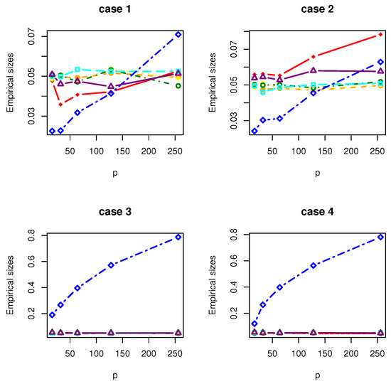
Figure 1.
The Empirical sizes of , , , , , and under normal distribution.
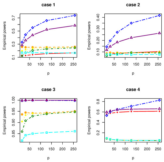
Figure 2.
The Empirical powers of , , , , , and under normal distribution.
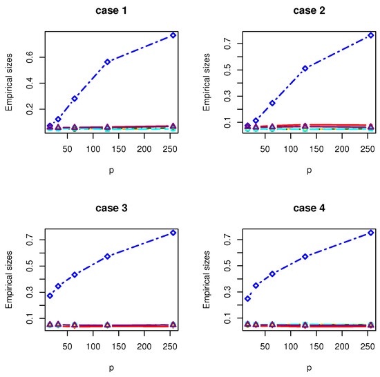
Figure 3.
The Empirical sizes of , , , , , and under normal distribution.
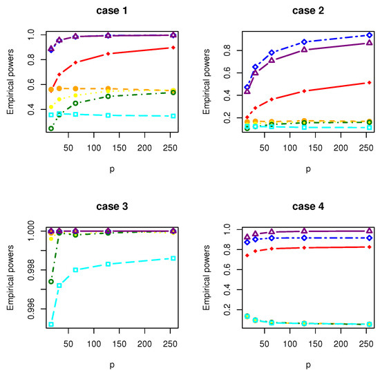
Figure 4.
The Empirical powers of , , , , , and under normal distribution.
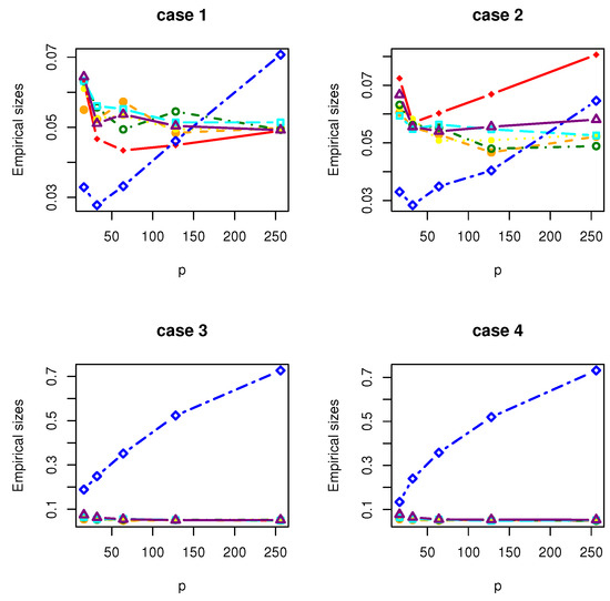
Figure 5.
The Empirical sizes of , , , , , and under Gamma distribution.
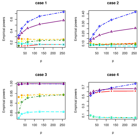
Figure 6.
The Empirical powers of , , , , , and under Gamma distribution.
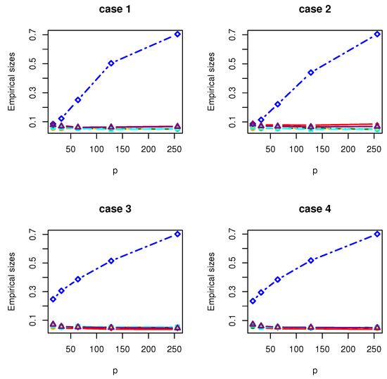
Figure 7.
The Empirical sizes of , , , , , and under Gamma distribution.
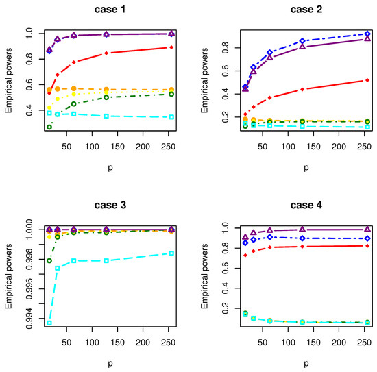
Figure 8.
The Empirical powers of , , , , , and under Gamma distribution.
In summary, our proposed test can control a given size reasonably and has greater powers than competing tests in all cases of our simulation whenever samples are from the normal model or the non-normal model. However, fails in controlling a given size. , , seriously deflates the empirical powers in some cases of our simulations. can slightly inflate the empirical size in some cases of our simulation.
5. Real Data Analysis
This problem will arise from the analysis of gene expression data. It was shown in [3] that many genes have different variances in gene expressions between disease states. For example, the dataset of the breast cancer of patient is classified into three groups based on their gene expression signatures: well-differentiated tumors ( = 29), moderately differentiated tumors ( = 136), and poorly differentiated and undifferentiated tumors ( = 35). The breast cancer microarray data sets, including patient outcome information, were downloaded from the National Center for Biotechnology Information (NCBI) Gene Expression Omnibus (GEO) data repository and are accessible through GEO Series accession now. GSE11121 (https://www.ncbi.nlm.nih.gov/geo/query/acc.cgi?acc=GSE11121, accessed on 26 June 2022). This dataset includes 200 samples, which is far fewer than data dimension 22,283. For this gene dataset, we are interested in checking whether the covariance matrices of the three groups are the same or not. It is noted that an important assumption for multivariate analysis of variance is that of equal covariance matrices in different groups. Therefore, testing the equality of several covariance matrices is necessary.
Since we used the raw breast cancer dataset (22,283 features), there are many features and no preprocessing. First, we preprocessed and filtered the data, including conventional preprocessing such as background adjustment, normalization, and summarization. Then, we performed feature screening, filtered out features whose coefficient of variation is out of range (0.25, 1.0) and controlled at least 5 samples to exceed 1320 count values. Finally, a data set of 200 samples and 1280 features was screened out, and then a high-dimensional hypothesis test problem was performed on the screened data set.
Compared with other methods and our method, the observed test statistics (p value) of the screened breast cancer dataset are , , , , , and . The p-values of the comparison method statistics , and our method’s statistic are significant.
6. Concluding Remarks
In this paper, we propose a new test on the homogeneity of k-sample covariance matrices in a high-dimensional setting. The asymptotic properties of the proposed test are derived under some regularity conditions. We compare our new test with six competing tests by simulation. Numerical results show that our proposed test can control the nominal size reasonably and that it has the highest empirical powers in our simulation scenario. However, just as what we showed in Section 2, the technique condition (C2) may not hold again when covariance matrices have some spiked eigenvalues. How to obtain the theoretical results of test statistics under spiked covariance matrices structure is an interested problem. We leave this problem as a future research direction.
Author Contributions
Conceptualization, P.S., Y.T. and M.C.; Simulation studies, P.S.; Formal analysis, P.S.; Funding acquisition, Y.T.; Investigation, P.S.; Methodology, P.S. and M.C.; Supervision, Y.T.; Software, P.S.; Visualization, P.S.; Validation, P.S. and M.C.; Writing—original draft, P.S.; Writing—review & editing, P.S. and M.C. All authors have read and agreed to the published version of the manuscript.
Funding
Tang’s research is supported by the Natural Science Foundation of China (No. 12271168) and the 111 Project of China (No. B14019). Cao’s research is supported by the Humanities and Social Sciences Foundation of Ministry of Education (No. 22YJC910001), the Natural Science Foundation of Anhui Province (No. 2108085MA09), the Foundation for Excellent Young Talents in College of Anhui Province (No. gxyqZD2021092) and the Program for Mathematical Statistics Research Team of Anhui Province (No. 2020jxtd102).
Data Availability Statement
Gene expression data generated for this manuscript is available to download and explore at https://www.ncbi.nlm.nih.gov/geo/query/acc.cgi?acc=GSE11121, accessed on 26 June 2022. All raw data are available in GEO database under the accession number GEO: GSE11121.
Conflicts of Interest
On behalf of the authors, the corresponding author states that there is no conflict of interest.
Appendix A. Some Lemmas
As mentioned in Section 3, we can assume all the population means are 0. In this case, we only need to consider respectively the first terms and of and in (5) and (6). Let , then we only need to prove the asymptotic normality of . To do this, we define , where and for and . A sequence of increasing -fields is defined as and for . Let denote the conditional expectation with respect to and . It is easy to obtain .
Lemma A1.
For any n, is a square integrable martingale difference sequence.
Proof.
The conclusion is obvious. Hence, the proof is omitted. □
Therefore, to prove Theorem 1, we next apply the martingale central limit theorem.
Lemma A2.
Under conditions (C1) and (C2), as ,
Proof.
By some calculations, we have
where
Note that . Next, we prove
Note that
It then follows that
where . In the following, we will prove for and 4.
Similarly,
We can obtain for and 4 by a similar method. It is noted that since and are non random.
As a result, it follows from the above equalities that
Finally, using similar calculations, we can obtain
This completes the proof of Lemma A2. □
Lemma A3.
Under the condition (C2), as ,
Proof.
By some calculations, for some constants and , we can obtain
and
As a result,
This completes the proof of Lemma A3. □
Appendix B. Proof of Theorem 1
Proof.
According Lemmas A1–A3, as , it is easy to complete the proof of Theorem 1. □
References
- Anderson, T.W. An Introduction to Multivariate Statistical Analysis, 3rd ed.; Wiley: Hoboken, NJ, USA, 2003. [Google Scholar]
- Muirhead, R.J. Aspects of Multivariate Statistical Theory; Wiley: New York, NY, USA, 2005. [Google Scholar]
- Schmidt, M.; Böhm, D.; Törne, C.; Steiner, E.; Puhl, A.; Pilch, H.; Lehr, H.; Hengstler, J.; Kölbl, H.; Gehrmann, M. The humoral immune system has a key prognostic impact in node-negative breast cancer. Cancer Res. 2008, 68, 5405–5413. [Google Scholar] [CrossRef] [PubMed]
- Khan, J.; Wei, J.S.; Ringner, M.; Saal, L.H.; Ladanyi, M.; Westermann, F.; Berthold, F.; Schwab, M.; Antonescu, C.R.; Peterson, C.; et al. Classification and diagnostic prediction of cancers using gene expression profiling and artificial neural networks. Nat. Med. 2001, 7, 673–679. [Google Scholar] [CrossRef] [PubMed]
- Zhu, Z.; Ong, Y.S.; Dash, M. Markov blanket-embedded genetic algorithm for gene selection. Pattern Recognit. 2007, 49, 3236–3248. [Google Scholar] [CrossRef]
- Li, T.; Zhang, C.; Ogihara, M. A comparative study of feature selection and multiclass classification methods for tissue classification based on gene expression. Bioinformatics 2004, 20, 2429–2437. [Google Scholar] [CrossRef] [PubMed]
- Wilks, S.S. Sample criteria for testing equality of means, equality of variances, and equality of covariances in a normal multivariate distribution. Ann. Math. Stat. 1946, 17, 257–281. [Google Scholar] [CrossRef]
- Ahmad, M.R. Testing homogeneity of several covariance matrices and multi-sample sphericity for high-dimensional data under non-normality. Commun. Stat. Theory Methods 2017, 46, 3738–3753. [Google Scholar] [CrossRef]
- Schott, J.R.A. Test for the equality of covariance matrices when the dimension is large relative to the sample sizes. Comput. Stat. Data Anal. 2007, 51, 6535–6542. [Google Scholar] [CrossRef]
- Srivastava, M.S.; Yanagihara, H. Testing the equality of several covariance matrices with fewer observations than the dimension. J. Multivar. Anal. 2010, 101, 1319–1329. [Google Scholar] [CrossRef]
- Zhang, C.; Bai, Z.; Hu, J.; Wang, C. Multi-sample test for high-dimensional covariance matrices. Commun. Stat. Theory Methods 2018, 47, 3161–3177. [Google Scholar] [CrossRef]
- Zhong, P.; Li, R.; Shanto, S. Homogeneity tests of covariance matrices with high-dimensional longitudinal data. Biometrika 2019, 106, 619–634. [Google Scholar] [CrossRef] [PubMed]
- Zheng, S.; Lin, R.; Guo, J.; Yin, G. Testing homogeneity of high-dimensional covariance matrices. Stat. Sin. 2020, 30, 35–53. [Google Scholar] [CrossRef]
- Qayed, A.; Han, D. Homogeneity test of several covariance matrices with high-dimensional data. J. Biopharm. Stat. 2021, 31, 523–540. [Google Scholar] [CrossRef] [PubMed]
- Box, G.E.P. A general distribution theory for a class of likelihood criteria. Biometrika 1949, 36, 317–346. [Google Scholar] [CrossRef]
- Li, J.; Chen, S. Two sample tests for high-dimensional covariance matrices. Ann. Stat. 2012, 40, 908–940. [Google Scholar] [CrossRef]
- Aoshima, M.; Yata, K. Two-sample tests for high-dimension, strongly spiked eigenvalue models. Stat. Sin. 2018, 28, 43–62. [Google Scholar] [CrossRef]
- Jiang, Y.; Wen, C.; Jiang, Y.; Wang, X.; Zhang, H. Use of Random Integration to Test Equality of High Dimensional Covariance Matrices. Stat. Sin. 2020. [Google Scholar] [CrossRef]
- Chen, S.; Qin, Y. A two-sample test for high-dimensional data with applications to gene-set testing. Ann. Stat. 2010, 38, 808–835. [Google Scholar] [CrossRef]


Publisher’s Note: MDPI stays neutral with regard to jurisdictional claims in published maps and institutional affiliations. |
© 2022 by the authors. Licensee MDPI, Basel, Switzerland. This article is an open access article distributed under the terms and conditions of the Creative Commons Attribution (CC BY) license (https://creativecommons.org/licenses/by/4.0/).