A Class of Semilinear Parabolic Problems and Analytic Semigroups ^†

Abstract

(1) Background: This paper is devoted to the study of a class of semilinear initial boundary value problems of parabolic type. (2) Methods: We make use of fractional powers of analytic semigroups and the interpolation theory of compact linear operators due to Lions–Peetre. (3) Results: We give a functional analytic proof of the $C^2$ compactness of a bounded regular solution orbit for semilinear parabolic problems with Dirichlet, Neumann and Robin boundary conditions. (4) Conclusions: As an application, we study the dynamics of a population inhabiting a strongly heterogeneous environment that is modeled by a class of diffusive logistic equations with Dirichlet and Neumann boundary conditions.

1. Introduction and Main Theorem

Let $\mathrm{\Omega }$ be a bounded domain of Euclidean space ${\mathbf{R}}^n$, with $C^{\infty }$ boundary $\Gamma =\partial \mathrm{\Omega }$; its closure $\overline{\mathrm{\Omega }}=\mathrm{\Omega }\cup \Gamma$ is an n-dimensional, compact $C^{\infty }$ manifold with boundary. We let

$$Au=\sum _{j,k=1}^n{a}^{jk}\left(x\right){\displaystyle \frac{{\partial }^{2}u}{\partial x_j\partial x_k}}+\sum _{j=1}^n{b}^j\left(x\right){\displaystyle \frac{\partial u}{\partial x_j}}+c\left(x\right)u$$

be a second-order, strictly elliptic differential operator with real coefficients on $\overline{\mathrm{\Omega }}$ = $\mathrm{\Omega }\cup \Gamma$ such that:

(1)

$a^{jk}\in C^{\infty }\left(\overline{\mathrm{\Omega }}\right)$ and $a^{jk}\left(x\right)=a^{kj}\left(x\right)$ for all $x\in \overline{\mathrm{\Omega }}$ and all $1\le j,k\le n$, and there exists a constant $a_0>0$ such that

$$\sum _{j,k=1}^n{a}^{jk}\left(x\right){\xi }_j{\xi }_k\ge c_0{\left|\xi \right|}^2\mathrm{f}\mathrm{o}\mathrm{r} \mathrm{a}\mathrm{l}\mathrm{l}(x,\xi )\in T^{*}\left(\overline{\mathrm{\Omega }}\right)=\overline{\mathrm{\Omega }}\times {\mathbf{R}}^n,$$

where $T^{*}\left(\overline{\mathrm{\Omega }}\right)$ is the cotangent bundle of $\overline{\mathrm{\Omega }}$.

(2)

$b^j\in C^{\infty }\left(\overline{\mathrm{\Omega }}\right)$ for all $1\le j\le n$.

(3)

$c\in C^{\infty }\left(\overline{\mathrm{\Omega }}\right)$ and $c\left(x\right)\le 0$ in $\mathrm{\Omega }$.

For simplicity, we suppose that:

$$\mathrm{The} \mathrm{function}c\left(x\right) \mathrm{does\; not\; vanish} identically \mathrm{in}\mathrm{\Omega }.$$

First, we study the following linear elliptic boundary value problem: Given functions $f\left(x\right)$ and $\phi \left(x^{\prime }\right)$ defined in $\mathrm{\Omega }$ and on $\Gamma$, respectively, find a function $u\left(x\right)$ in $\mathrm{\Omega }$ such that

$$\left\{\begin{array}{cc}Au=f\hfill & \mathrm{in} \mathrm{\Omega },\hfill \\ Bu:=a\left(x^{\prime }\right){\displaystyle \frac{\partial u}{\partial \nu }}+b\left(x^{\prime }\right)u=\phi \hfill & \mathrm{on} \Gamma .\hfill \end{array}\right.$$

(1)

Here:

(1)

$a\left(x^{\prime }\right)$ and $b\left(x^{\prime }\right)$ are real-valued, $C^{\infty }$ functions on $\Gamma$.

(2)

$\partial /\partial \nu$ is the conormal derivative associated with the differential operator A:

$${\displaystyle \frac{\partial }{\partial \nu }}=\sum _{j,k=1}^n{a}^{jk}\left(x^{\prime }\right)n_k{\displaystyle \frac{\partial }{\partial x_j}},$$

$\mathbf{n}=\left(n_1,n_2,\dots ,n_n\right)$ being the unit outward normal to the boundary $\Gamma$ (see Figure 1).

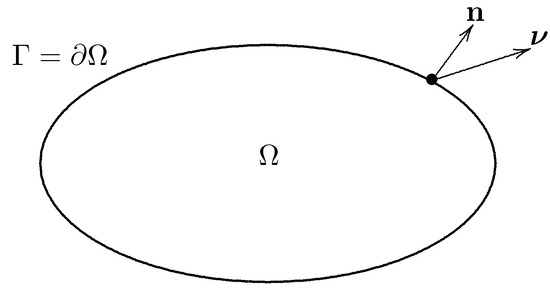Figure 1. The unit outward normal $\mathbf{n}$ and the conormal $\nu$ to $\Gamma$.

We associate with the linear problem (1) an unbounded linear operator ${\mathfrak{A}}_p$ from the Banach space $L^p\left(\mathrm{\Omega }\right)$ into itself as follows (see [1], Theorem 1.2):

(a)

The domain $D\left({\mathfrak{A}}_p\right)$ of definition of ${\mathfrak{A}}_p$ is the set

$$D\left({\mathfrak{A}}_p\right)=\left\{u\in W^{2,p}\left(\mathrm{\Omega }\right):Bu=a\left(x^{\prime }\right){\displaystyle \frac{\partial u}{\partial \nu }}+b\left(x^{\prime }\right)u=0\mathrm{on} \Gamma \right\}.$$

(2)

(b)

${\mathfrak{A}}_{p}u=Au$ for every $u\in D\left({\mathfrak{A}}_p\right)$.

Then we have the following proposition (see [1], Lemma 8.1):

Proposition 1. 

Let $1<p<\infty$. Suppose that the following conditions (H.1) and (H.2) are satisfied:

(H.1) 

$a\left(x^{\prime }\right)\ge 0$ and $b\left(x^{\prime }\right)\ge 0$ on Γ.

(H.2) 

$a\left(x^{\prime }\right)+b\left(x^{\prime }\right)>0$ on Γ.

Then we have the global a priori estimate

$${\parallel u\parallel }_{W^{2,p}\left(\mathrm{\Omega }\right)}\le C{∥Au∥}_{L^p\left(\mathrm{\Omega }\right)}\mathit{for\; all} u\in D\left({\mathfrak{A}}_p\right).$$

(3)

Moreover, we have the following generation theorem for analytic semigroups in the framework of $L^p$ Sobolev spaces (see [1], Theorem 1.2):

Theorem 1

(the generation theorem for analytic semigroups). Let $1<p<\infty$. If the conditions (H.1) and (H.2) are satisfied, then we have the following two assertions (i) and (ii):

(i) 

For every $0<\epsilon <\pi /2$, there exists a constant $r\left(\epsilon \right)>0$ such that the resolvent set of ${\mathfrak{A}}_p$ contains the set

$$\Sigma \left(\epsilon \right)=\left\{\lambda =r^2{e}^{i\theta }:r\ge r\left(\epsilon \right),\left|\theta \right|\le \pi -\epsilon \right\},$$

and that the resolvent ${({\mathfrak{A}}_p-\lambda I)}^{-1}$ satisfies the estimate

$$∥{\left({\mathfrak{A}}_p-\lambda I\right)}^{-1}∥\le {\displaystyle \frac{c_p\left(\epsilon \right)}{\left|\lambda \right|}}\mathit{for\; all} \lambda \in \Sigma \left(\epsilon \right),$$

(4)

where $c_p\left(\epsilon \right)>0$ is a constant depending on ε.

(ii) 

The operator ${\mathfrak{A}}_p$ generates a semigroup $U\left(z\right)=e^{z{\mathfrak{A}}_p}$ on the space $L^p\left(\mathrm{\Omega }\right)$ which is analytic in the sector

$${\Delta }_{\epsilon }=\left\{z=t+is:z\ne 0,|argz|<\pi /2-\epsilon \right\}$$

for any $0<\epsilon <\pi /2$ (see Figure 2).

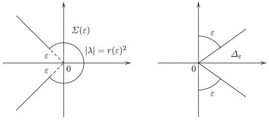Figure 2. The set $\Sigma \left(\epsilon \right)$ and the sector ${\Delta }_{\epsilon }$.

1.1. Statement of Main Theorem

Now let $g\left(t\right)$ be a real-valued, locally Lipschitz continuous function on $\mathbf{R}$. In this section we consider the following semilinear initial boundary value problem of parabolic type:

$$\left\{\begin{array}{cc}\frac{\partial u}{\partial t}-Au=g\left(u\right)\hfill & \mathit{in} \mathrm{\Omega }\times (0,\infty ),\hfill \\ Bu=a\left(x^{\prime }\right)\frac{\partial u}{\partial \nu }+b\left(x^{\prime }\right)u=0\hfill & \mathit{on} \Gamma \times (0,\infty ),\hfill \\ u(x,0)=u_0\hfill & \mathit{in} \overline{\mathrm{\Omega }}.\hfill \end{array}\right.$$

(5)

A function $u(x,t)$ is called a regular solution of the semilinear problem (5) if it belongs to the space $C^{2+\beta ,1+\beta /2}\left(\overline{\mathrm{\Omega }}\times [0,\infty )\right)$ for $0<\beta <1$:

$$\begin{array}{cc}\hfill & C^{2+\beta ,1+\beta /2}\left(\overline{\mathrm{\Omega }}\times [0,\infty )\right)\hfill \\ \hfill :=& \mathrm{the\; space\; of\; continuously\; differentiable\; functions}\hfill \\ \hfill & u(x,t)\in C\left(\overline{\mathrm{\Omega }}\times [0,\infty )\right) \mathrm{twice\; with\; respect\; to} x \mathrm{and\; once}\hfill \\ \hfill & \mathrm{with\; respect\; to} t \mathrm{such\; that} {\partial }_{x}u(x,t) \mathrm{are} (1+\beta )/2-\mathrm{H}\mathrm{ö}\mathrm{l}\mathrm{d}\mathrm{e}\mathrm{r}\hfill \\ \hfill & \mathrm{continuous\; with\; respect\; to} t, \mathrm{that} {\partial }_{t}u(x,t) \mathrm{is} \beta -\mathrm{H}\mathrm{ö}\mathrm{l}\mathrm{d}\mathrm{e}\mathrm{r}\hfill \\ \hfill & \mathrm{continuous\; with\; respect\; to} x \mathrm{and} \beta /2-\mathrm{H}\mathrm{ö}\mathrm{l}\mathrm{d}\mathrm{e}\mathrm{r} \mathrm{continuous}\hfill \\ \hfill & \mathrm{with\; respect\; to} t \mathrm{and\; further\; that} {\partial }_x^{2}u(x,t)\mathrm{are} \beta -\mathrm{H}\mathrm{ö}\mathrm{l}\mathrm{d}\mathrm{e}\mathrm{r}\hfill \\ \hfill & \mathrm{continuous\; with\; respect\; to} x \mathrm{and} \beta /2-\mathrm{H}\mathrm{ö}\mathrm{l}\mathrm{d}\mathrm{e}\mathrm{r} \mathrm{continuous}\hfill \\ \hfill & \mathrm{with\; respect\; to} t.\hfill \end{array}$$

By using the operator ${\mathfrak{A}}_p$ defined by Formula (2), we can rewrite the semilinear initial boundary value problem (5) in the following abstract semilinear Cauchy problem:

$$\left\{\begin{array}{cc}\frac{\partial u}{\partial t}={\mathfrak{A}}_{p}u+g\left(u\right)\hfill & \mathrm{in} (0,\infty ),\hfill \\ u\left(0\right)=u_0.\hfill \end{array}\right.$$

(6)

In this paper, in the light of the interpolation theory of compact linear operators due to Lions–Peetre [2] we give a functional analytic proof of the following $C^2$ compactness of a bounded regular solution orbit of the semilinear Cauchy problem (6) (cf. [3], Satz):

Theorem 2.

Suppose that the following conditions (H.1) and (H.3) are satisfied:

(H.1) 

$a\left(x^{\prime }\right)\ge 0$ and $b\left(x^{\prime }\right)\ge 0$ on Γ.

(H.3) 

Either $a\left(x^{\prime }\right)>0$ on Γ (regular Robin and Neumann cases) or $a\left(x^{\prime }\right)\equiv 0$ and $b\left(x^{\prime }\right)>0$ on Γ (Dirichlet case).

Let $n<p<\infty$ and

$$\frac{1}{2}+\frac{n}{2p}<\alpha <1.$$

(7)

If $u_0\in C^{2+\alpha }\left(\overline{\mathrm{\Omega }}\right)$ such that $Bu=0$ on Γ and if $0<\beta <2\alpha -1-\frac{n}{p}$, then the Hölder norm ${∥u\left(t\right)∥}_{C^{2+\beta }\left(\overline{\mathrm{\Omega }}\right)}$ of a bounded regular solution $u(·,t)$ of the semilinear Cauchy problem (6) isuniformly boundedfor all $t\ge 0$. In particular, the orbit of a bounded regular solution $u(·,t)$ is relatively compact in the space $C^2\left(\overline{\mathrm{\Omega }}\right)$.

1.2. Outline of the Paper

The rest of this paper is organized as follows.

Section 2 is devoted to the Hille–Yosida theory of analytic semigroups which forms a functional analytic background for the proof of Theorem 2. We consider fractional powers ${\left(-{\mathfrak{A}}_p\right)}^{\alpha }$ of the infinitesimal generator ${\mathfrak{A}}_p$ for $0<\alpha \le 1$ (see Formulas (9) and (10)), and summarize some basic facts about the fractional powers ${\left(-{\mathfrak{A}}_p\right)}^{\alpha }$ and the analytic semigroup $U\left(t\right)=e^{t{\mathfrak{A}}_p}$. In particular, we study the imbedding characteristics of the spaces $D\left({\left(-{\mathfrak{A}}_p\right)}^{\alpha }\right)$, which make these spaces so useful in the study of the solution $u\left(t\right)$ of the semilinear Cauchy problem (6) (Lemmas 1–3).

In Section 3, we formulate the interpolation theory of compact linear operators of Lions–Peetre [2] (Theorem 3) in order to give a functional analytic proof of Theorem 2 (Theorem 4 and Corollary 1). This section is the heart of the subject.

In Section 4, we give the proof of Theorem 2. In view of the Ascoli–Arzelà theorem, we have only to show that, for some $0<\beta <1$ the Hölder norm ${∥u\left(t\right)∥}_{C^{2+\beta }\left(\overline{\mathrm{\Omega }}\right)}$ of a bounded regular solution orbit $u(·,t)$ of the semilinear Cauchy problem (6) is uniformly bounded for all $t\ge 0$. The proof is given by a series of claims (Claims 2–5). We make use of the classical elliptic Schauder theory for $t\ge 1$ and the classical linear parabolic theory for $0\le t\le 1$.

In Section 5, we study of the existence of positive solutions of semilinear Dirichlet and Neumann problems for diffusive logistic equations, which models population dynamics in environments with spatial heterogeneity (Theorems 5 and 6 for the Dirichlet case and Theorems 8 and 9 for the Neumann case). Moreover, as an application of Theorem 2 (see [4], Section 6), we discuss the stability properties for positive steady states (Theorem 7 for the Dirichlet case and Theorem 10 for the Neumann case). A biological interpretation of main theorems is that an initial population will grow exponentially until limited by a lack of available resources if the diffusion rate is below some critical value; this idea is generally credited to the English economist Thomas Robert Malthus (1766–1834). On the other hand, if the diffusion rate is above this critical value, then the model obeys the logistic equation introduced by the Belgian mathematical biologist Pierre François Verhulst (1804–1849). We remark that this critical value tends to be smaller in situations where favorable and unfavorable habits are closely intermingled, and larger when the favorable region consists of a relatively small number of relatively large isolated components (see Formula (69)).

In Appendix A we study linear initial boundary value problems of parabolic type in the framework of Hölder spaces, following Ladyzhenskaya et al. [5] and Friedman [6]. This makes the paper fairly self-contained.

2. Fractional Powers for Analytic Semigroups

By virtue of Theorem 1, we may suppose that the operator ${\mathfrak{A}}_p$, defined by Formula (2), satisfies the following two conditions:

(R.1)

The resolvent set of ${\mathfrak{A}}_p$ contains the region $\Sigma$ shown in Figure 3.

Figure 3. The region $\Sigma$ in condition (R.1).

(R.2)

There exists a constant $M>0$ such that the resolvent ${\left(\lambda I-{\mathfrak{A}}_p\right)}^{-1}$ satisfies the estimate (see estimate (4))

$$∥{\left(\lambda I-{\mathfrak{A}}_p\right)}^{-1}∥\le {\displaystyle \frac{M}{1+\left|\lambda \right|}}\mathrm{for\; all} \lambda \in \Sigma .$$

(8)

Thus, we can define the fractional powers ${(-{\mathfrak{A}}_p)}^{-\alpha }$ and ${(-{\mathfrak{A}}_p)}^{\alpha }$ for $0<\alpha <1$ as follows:

$$\begin{array}{cc}\hfill {\left(-{\mathfrak{A}}_p\right)}^{-\alpha }u& =-{\displaystyle \frac{sin\alpha \pi }{\pi }}{\int }_0^{\infty }{s}^{-\alpha }{\left({\mathfrak{A}}_p-sI\right)}^{-1}uds\hfill \\ \hfill & ={\displaystyle \frac{sin\alpha \pi }{\pi }}{\int }_0^{\infty }{s}^{-\alpha }{\left(sI-{\mathfrak{A}}_p\right)}^{-1}uds\mathrm{for\; all} \in L^p\left(\mathrm{\Omega }\right),\hfill \end{array}$$

(9)

and

$${\left(-{\mathfrak{A}}_p\right)}^{\alpha }= \mathrm{the\; inverse\; of} {(-{\mathfrak{A}}_p)}^{-\alpha }.$$

Remark that the operator ${(-{\mathfrak{A}}_p)}^{\alpha }$ is a closed linear operator with domain

$$D\left({(-{\mathfrak{A}}_p)}^{\alpha }\right)\supset D\left(-{\mathfrak{A}}_p\right)=D\left({\mathfrak{A}}_p\right),$$

and further that

$$\begin{array}{cc}\hfill {\left(-{\mathfrak{A}}_p\right)}^{\alpha }u& ={\displaystyle \frac{sin\alpha \pi }{\pi }}{\int }_0^{\infty }{s}^{\alpha -1}{\left({\mathfrak{A}}_p-sI\right)}^{-1}{\mathfrak{A}}_{p}uds\hfill \\ \hfill & ={\displaystyle \frac{sin\alpha \pi }{\pi }}{\int }_0^{\infty }{s}^{\alpha -1}{\left(sI-{\mathfrak{A}}_p\right)}^{-1}\left(-{\mathfrak{A}}_{p}u\right)ds\mathrm{for\; all} u\in D\left({\mathfrak{A}}_p\right).\hfill \end{array}$$

(10)

In this section, we study the imbedding characteristics of the spaces $D\left({\left(-{\mathfrak{A}}_p\right)}^{\alpha }\right)$, which will make these spaces so useful in the study of semilinear parabolic differential equations. For detailed studies of this subject, the reader might be referred to Henry [7], Pazy [8], Lunardi [9] and Amann [10].

We let

$$\begin{array}{cc}\hfill {\mathcal{X}}_{\alpha }:=& \mathrm{the\; space} D\left({\left(-{\mathfrak{A}}_p\right)}^{\alpha }\right) \mathrm{endowed\; with\; the} graph norm {\parallel · \parallel }_{\alpha }\hfill \\ \hfill & \mathrm{of\; the\; fractional\; power} {\left(-{\mathfrak{A}}_p\right)}^{\alpha } \mathrm{for} 0<\alpha <1,\hfill \end{array}$$

(11)

and

$$\begin{array}{cc}\hfill & {\mathcal{X}}_0:=L^p\left(\mathrm{\Omega }\right),\hfill \\ \hfill & {\mathcal{X}}_1:=D\left(-{\mathfrak{A}}_p\right)=D\left({\mathfrak{A}}_p\right).\hfill \end{array}$$

Here

$${∥u∥}_{\alpha }={\left({\parallel u\parallel }_{L^p\left(\mathrm{\Omega }\right)}^2+{∥{\left(-{\mathfrak{A}}_p\right)}^{\alpha }u∥}_{L^p\left(\mathrm{\Omega }\right)}^2\right)}^{1/2}\mathrm{for\; all} u\in D\left({\left(-{\mathfrak{A}}_p\right)}^{\alpha }\right).$$

(12)

Then we have the following three assertions (1), (2) and (3) (see Henry [7], Theorem 1.4.8; [1], Proposition 3.16):

(1)

The space ${\mathcal{X}}_{\alpha }$ is a Banach space.

(2)

By the a priori estimate (3), it follows that the graph norm ${\parallel u\parallel }_{\alpha }$ is equivalent to the norm ${∥{(-{\mathfrak{A}}_p)}^{\alpha }u∥}_{L^p\left(\mathrm{\Omega }\right)}$:

$${∥u∥}_{\alpha }\approx {∥{\left(-{\mathfrak{A}}_p\right)}^{\alpha }u∥}_{L^p\left(\mathrm{\Omega }\right)}\mathrm{for\; all} u\in D\left({\left(-{\mathfrak{A}}_p\right)}^{\alpha }\right).$$

(13)

(3)

If $0\le \alpha <\beta \le 1$, then we have ${\mathcal{X}}_{\beta }\subset {\mathcal{X}}_{\alpha }$ with continuous injection.

Moreover, we recall the following fundamental inequlaities for analytic semigroups ([7], Theorems 1.3.4 and 1.4.3; [1], Remark 3.1):

$$\begin{array}{cc}\hfill & ∥e^{t{\mathfrak{A}}_p}∥\le C_1{e}^{-\delta t}\mathrm{for\; all} t\ge 0.\hfill \end{array}$$

(14)

$$\begin{array}{cc}\hfill & ∥{\left(-{\mathfrak{A}}_p\right)}^{\alpha }{e}^{t{\mathfrak{A}}_p}∥\le \frac{C\left(\alpha \right)}{t^{\alpha }}{e}^{-\delta t}\mathrm{for\; all} t>0,\hfill \end{array}$$

(15)

$$\begin{array}{cc}\hfill & ∥\left(e^{t{\mathfrak{A}}_p}-I\right){\left(-{\mathfrak{A}}_p\right)}^{-1}∥\le C_{2}t\mathrm{for\; all} t\ge 0.\hfill \end{array}$$

(16)

It is easy to verify that every solution $u\left(t\right)$ of the abstract semilinear Cauchy problem (6) is given by the following integral formula

$$u\left(t\right)=e^{t{\mathfrak{A}}_p}{u}_0+{\int }_0^t{e}^{(t-s){\mathfrak{A}}_p}f\left(s\right)ds\mathrm{for\; all} t\ge 0,$$

(17)

with

$$f\left(t\right):=g\left(u\left(t\right)\right)\mathrm{for} t\ge 0.$$

If the orbit of a regular solution $u\left(t\right)$ of the semilinear problem (5) is bounded, then we can find constants $K>0$ and $L>0$ such that

$$\begin{array}{cc}\hfill & {∥f\left(t\right)∥}_{L^p\left(\mathrm{\Omega }\right)}\le K\mathrm{for\; all} t\ge 0,\hfill \end{array}$$

(18)

$$\begin{array}{cc}\hfill & {∥f\left(s\right)-f\left(t\right)∥}_{L^p\left(\mathrm{\Omega }\right)}\le L{∥u\left(s\right)-u\left(t\right)∥}_{L^p\left(\mathrm{\Omega }\right)}\mathrm{for\; all} s,t\ge 0.\hfill \end{array}$$

(19)

Indeed, it suffices to note that the function

$$\mathbf{R}\ni s⟼f\left(s\right)=g\left(u\left(s\right)\right)$$

is bounded and Lipschitz continuous if the uniform norm ${\parallel u(·,s)\parallel }_{C(\overline{\mathrm{\Omega }})}$ is bounded for all $s\ge 0$.

First, we prove the ${\mathcal{X}}_{\alpha }$-boundedness of the solution $u\left(t\right)$ of the abstract semilinear Cauchy problem (6) (cf. [1], Theorem 3.18):

Lemma 1.

Let $u_0\in D\left({\mathfrak{A}}_p\right)$ and $0<\alpha <1$. If the conditions (R.1) and (R.2) are satisfied, then we have, for all $t\ge 0$,

$$\begin{array}{cc}\hfill & u\left(t\right)\in {\mathcal{X}}_{\alpha }=D\left({\left(-{\mathfrak{A}}_p\right)}^{\alpha }\right),\hfill \end{array}$$

(20)

$$\begin{array}{cc}\hfill & {∥u\left(t\right)∥}_{\alpha }\le C_1\left(\alpha \right),\hfill \end{array}$$

(21)

with a constant $C_1\left(\alpha \right)>0$. For example, we may take

$$C_1\left(\alpha \right):=C_1{∥u_0∥}_{\alpha }+C\left(\alpha \right)K\frac{\Gamma (1-\alpha )}{{\delta }^{1-\alpha }}.$$

Proof. 

Since the fractional power ${\left(-{\mathfrak{A}}_p\right)}^{\alpha }$ is a closed operator and since

$$u_0\in D\left({\mathfrak{A}}_p\right)\subset D\left({\left(-{\mathfrak{A}}_p\right)}^{\alpha }\right),$$

it follows from the integral Formula (17) that

$$\begin{array}{cc}\hfill & {\left(-{\mathfrak{A}}_p\right)}^{\alpha }u\left(t\right)={\left(-{\mathfrak{A}}_p\right)}^{\alpha }{e}^{t{\mathfrak{A}}_p}{u}_0+{\left(-{\mathfrak{A}}_p\right)}^{\alpha }\left({\int }_0^t{e}^{(t-s){\mathfrak{A}}_p}f\left(s\right)ds\right)\hfill \\ \hfill & ={\left(-{\mathfrak{A}}_p\right)}^{\alpha }{e}^{t{\mathfrak{A}}_p}{u}_0+{\int }_0^t{\left(-{\mathfrak{A}}_p\right)}^{\alpha }{e}^{(t-s){\mathfrak{A}}_p}f\left(s\right)ds\hfill \\ \hfill & =e^{t{\mathfrak{A}}_p}{\left(-{\mathfrak{A}}_p\right)}^{\alpha }{u}_0+{\int }_0^t{\left(-{\mathfrak{A}}_p\right)}^{\alpha }{e}^{(t-s){\mathfrak{A}}_p}f\left(s\right)ds\mathrm{for\; all} t\ge 0.\hfill \end{array}$$

Hence, by using inequalities (15) and (18) we obtain that

$$\begin{array}{cc}\hfill {∥u\left(t\right)∥}_{\alpha }& ={∥{\left(-{\mathfrak{A}}_p\right)}^{\alpha }u\left(t\right)∥}_{L^p\left(\mathrm{\Omega }\right)}\hfill \\ \hfill & ={∥e^{t{\mathfrak{A}}_p}{\left(-{\mathfrak{A}}_p\right)}^{\alpha }{u}_0+{\int }_0^t{\left(-{\mathfrak{A}}_p\right)}^{\alpha }{e}^{(t-s){\mathfrak{A}}_p}f\left(s\right)ds∥}_{L^p\left(\mathrm{\Omega }\right)}\hfill \\ \hfill & \le {∥e^{t{\mathfrak{A}}_p}·{\left(-{\mathfrak{A}}_p\right)}^{\alpha }{u}_0∥}_{L^p\left(\mathrm{\Omega }\right)}+{\int }_0^t{∥{\left(-{\mathfrak{A}}_p\right)}^{\alpha }{e}^{(t-s){\mathfrak{A}}_p}f\left(s\right)∥}_{L^p\left(\mathrm{\Omega }\right)}ds\hfill \\ \hfill & \le ∥e^{t{\mathfrak{A}}_p}∥·{∥{\left(-{\mathfrak{A}}_p\right)}^{\alpha }{u}_0∥}_{L^p\left(\mathrm{\Omega }\right)}+{\int }_0^t{∥{\left(-{\mathfrak{A}}_p\right)}^{\alpha }{e}^{(t-s){\mathfrak{A}}_p}f\left(s\right)∥}_{L^p\left(\mathrm{\Omega }\right)}ds\hfill \\ \hfill & \le C_1{e}^{-\delta t}{∥u_0∥}_{\alpha }+C\left(\alpha \right){\int }_0^t\frac{e^{-\delta (t-s)}}{{(t-s)}^{\alpha }}{∥f\left(s\right)∥}_{L^p\left(\mathrm{\Omega }\right)}ds\hfill \\ \hfill & \le C_1{e}^{-\delta t}{∥u_0∥}_{\alpha }+C\left(\alpha \right)K{\int }_0^t\frac{e^{-\delta (t-s)}}{{(t-s)}^{\alpha }}ds\hfill \\ \hfill & \le C_1{∥u_0∥}_{\alpha }+C\left(\alpha \right)K\frac{\Gamma (1-\alpha )}{{\delta }^{1-\alpha }}\hfill \\ \hfill & :=C_1\left(\alpha \right)\mathrm{for\; all} t\ge 0.\hfill \end{array}$$

The proof of Lemma 1 is complete. □

Secondly, we prove the boundedness of the difference

$${∥\frac{u(t+h)-u\left(t\right)}{h}∥}_{L^p\left(\mathrm{\Omega }\right)}$$

of the solution $u\left(t\right)$ of the abstract semilinear Cauchy problem (6):

Lemma 2.

Let $u_0\in D\left(-{\mathfrak{A}}_p\right)=D\left({\mathfrak{A}}_p\right)$. If the conditions (R.1) and (R.2) are satisfied, then there exists a constant $C>0$ such that

$${∥u(t+h)-u\left(t\right)∥}_{L^p\left(\mathrm{\Omega }\right)}\le Ch\mathit{for\; all} t\ge 0 \mathit{and} h>0.$$

(22)

Proof. 

The proof of Lemma 2 is divided into three steps.

Step 1: By using the integral Formula (17), we have, for $0\le \tau \le t$ and $h>0$,

$$\begin{array}{cc}\hfill & u(t+h)-u\left(t\right)\hfill \\ \hfill & =\left(e^{(t+h){\mathfrak{A}}_p}-e^{t{\mathfrak{A}}_p}\right)u_0+{\int }_{\tau }^{\tau +h}{e}^{(t+h-s){\mathfrak{A}}_p}f\left(s\right)ds\hfill \\ \hfill & +{\int }_0^{\tau }\left(e^{(t+h-s){\mathfrak{A}}_p}-e^{(t-s){\mathfrak{A}}_p}\right)f\left(s\right)ds+{\int }_{\tau }^t{e}^{(t-s){\mathfrak{A}}_p}\left(f(s+h)-f\left(s\right)\right)ds.\hfill \end{array}$$

(23)

However, we obtain from inequalities (14)–(16) that

$$\begin{array}{cc}\hfill & •{∥\left(e^{(t+h){\mathfrak{A}}_p}-e^{t{\mathfrak{A}}_p}\right)u_0∥}_{L^p\left(\mathrm{\Omega }\right)}\hfill \\ \hfill & ={∥\left(e^{h{\mathfrak{A}}_p}-I\right){\left(-{\mathfrak{A}}_p\right)}^{-1}·e^{t{\mathfrak{A}}_p}\left(\left(-{\mathfrak{A}}_p\right)u_0\right)∥}_{L^p\left(\mathrm{\Omega }\right)}\hfill \\ \hfill & \le C_{2}h{∥e^{t{\mathfrak{A}}_p}\left(\left(-{\mathfrak{A}}_p{u}_0\right)\right)∥}_{L^p\left(\mathrm{\Omega }\right)}\hfill \\ \hfill & \le C_{2}h{C}_1{e}^{-\delta t}∥\left(\left(-{\mathfrak{A}}_p\right)u_0\right)∥=C_1{C}_{2}h{e}^{-\delta t}{∥u_0∥}_1\hfill \\ \hfill & \le \left(C_1{C}_2{∥u_0∥}_1\right)h\hfill \\ \hfill & =C_{3}h\mathrm{for\; all} t\ge 0,\hfill \end{array}$$

(24)

where

$$C_3:=C_1{C}_2{∥u_0∥}_1,$$

and further from inequalities (18) and (19) that

$$\begin{array}{cc}\hfill & •{∥{\int }_{\tau }^{\tau +h}{e}^{(t+h-s){\mathfrak{A}}_p}f\left(s\right)ds∥}_{L^p\left(\mathrm{\Omega }\right)}\hfill \\ \hfill & \le {\int }_{\tau }^{\tau +h}{∥e^{(h-s){\mathfrak{A}}_p}f\left(s\right)∥}_{L^p\left(\mathrm{\Omega }\right)}ds·∥e^{t{\mathfrak{A}}_p}∥\hfill \\ \hfill & \le K{\int }_{\tau }^{\tau +h}{C}_1{e}^{-\delta (h-s)}ds·C_1{e}^{-\delta t}\hfill \\ \hfill & \le K{C}_1^2{\int }_{\tau -h}^{\tau }{e}^{\delta s}ds·e^{-\delta t}\hfill \\ \hfill & \le K{C}_1^2{e}^{-\delta t}·\frac{1}{\delta }{e}^{\tau \delta }\left(1-e^{-h\delta }\right)\hfill \\ \hfill & \le K{C}_1^2{e}^{-(t-\tau )\delta }\frac{1}{\delta }·h\delta =K{C}_1^2{e}^{-(t-\tau )\delta }h\hfill \\ \hfill & \le K{C}_1^{2}h\mathrm{for} 0\le \tau \le t,\hfill \end{array}$$

(25)

$$\begin{array}{cc}\hfill & •{∥{\int }_0^{\tau }\left(e^{(t+h-s){\mathfrak{A}}_p}-e^{(t-s){\mathfrak{A}}_p}\right)f\left(s\right)ds∥}_{L^p\left(\mathrm{\Omega }\right)}\hfill \\ \hfill & \le {\int }_0^{\tau }∥\left(-{\mathfrak{A}}_p\right)e^{(t-s){\mathfrak{A}}_p}·\left(e^{h{\mathfrak{A}}_p}-I\right){\left(-{\mathfrak{A}}_p\right)}^{-1}∥·{∥f\left(s\right)∥}_{L^p\left(\mathrm{\Omega }\right)}ds\hfill \\ \hfill & \le K{C}_{2}h{\int }_0^{\tau }∥\left(-{\mathfrak{A}}_p\right)e^{(t-s){\mathfrak{A}}_p}∥ds\hfill \\ \hfill & \le K{C}_{2}hC\left(1\right){\int }_0^{\tau }\frac{1}{t-s}{e}^{-\delta (t-s)}ds\hfill \\ \hfill & \le K{C}_{2}hC\left(1\right)\frac{e^{-\delta t}}{t-\tau }{\int }_0^{\tau }{e}^{\delta s}ds=K{C}_{2}h\frac{C\left(1\right)}{\delta }\frac{e^{-\delta t}}{t-\tau }\left(e^{\delta \tau }-1\right)\hfill \\ \hfill & \le K{C}_{2}h\frac{C\left(1\right)}{\delta }\frac{1}{t-\tau }\mathrm{for} 0\le \tau <t,\hfill \end{array}$$

(26)

$$\begin{array}{cc}\hfill & •{∥{\int }_{\tau }^t{e}^{(t-s){\mathfrak{A}}_p}\left(f(s+h)-f\left(s\right)\right)ds∥}_{L^p\left(\mathrm{\Omega }\right)}\hfill \\ \hfill & \le {\int }_{\tau }^t∥e^{(t-s){\mathfrak{A}}_p}∥·{∥f(s+h)-f\left(s\right)∥}_{L^p\left(\mathrm{\Omega }\right)}ds\hfill \\ \hfill & \le C_{1}L{\int }_{\tau }^t{e}^{-(t-s)\delta }{∥u(s+h)-u\left(s\right)∥}_{L^p\left(\mathrm{\Omega }\right)}ds\mathrm{for} 0\le \tau \le t.\hfill \end{array}$$

(27)

By combining inequalities (24) through (27), we have proved that

$$\begin{array}{cc}\hfill & {∥u(t+h)-u\left(t\right)∥}_{L^p\left(\mathrm{\Omega }\right)}\hfill \\ \hfill & \le \left(C_3+C_1^{2}K+\frac{C_{2}C\left(1\right)K}{\delta }\frac{1}{t-\tau }\right)h\hfill \\ \hfill & +C_{1}L{\int }_{\tau }^t{e}^{-(t-s)\delta }{∥u(s+h)-u\left(s\right)∥}_{L^p\left(\mathrm{\Omega }\right)}ds\mathrm{for} 0\le \tau <t.\hfill \\ \hfill & \le C_4\left(1+\frac{1}{t-\tau }\right)h+C_{1}L{\int }_{\tau }^t{e}^{-(t-s)\delta }{∥u(s+h)-u\left(s\right)∥}_{L^p\left(\mathrm{\Omega }\right)}ds\mathrm{for} 0\le \tau <t.\hfill \end{array}$$

(28)

Here

$$C_4:=max\left\{C_1{C}_2{∥u_0∥}_1+C_1^{2}K,\frac{C_{2}C\left(1\right)K}{\delta }\right\}.$$

Step 2: If we let

$$\varphi \left(t\right):=e^{\delta t}{∥u(t+h)-u\left(t\right)∥}_{L^p\left(\mathrm{\Omega }\right)}\mathrm{for} t\ge 0,$$

then we obtain from inequality (28) that

$$\begin{array}{cc}\hfill e^{-\delta t}\varphi \left(t\right)& ={∥u(t+h)-u\left(t\right)∥}_{L^p\left(\mathrm{\Omega }\right)}\hfill \\ \hfill & \le C_4\left(1+\frac{1}{t-\tau }\right)h+C_{1}L\left({\int }_{\tau }^t\varphi \left(s\right)ds\right)e^{-\delta t}\mathrm{for} 0\le \tau <t,\hfill \end{array}$$

so that

$$\begin{array}{cc}\hfill & e^{\delta t}{∥u(t+h)-u\left(t\right)∥}_{L^p\left(\mathrm{\Omega }\right)}=\varphi \left(t\right)\hfill \\ \hfill & \le C_{4}h\left(1+\frac{1}{t-\tau }\right)e^{\delta t}+C_{1}L{\int }_{\tau }^t\varphi \left(s\right)ds\mathrm{for} 0\le \tau <t.\hfill \end{array}$$

(29)

Now we need the following form of Gronwall’s inequality ([11], Lemma 29.2):

Claim 1

[Gronwall]. Let $g\left(t\right)$, $v\left(t\right)$ be continuous functions in $C[0,T]$, and let $h\left(t\right)$ be a non-negative, integrable function in $(0,T)$. Suppose that the following inequality holds true:

$$v\left(t\right)\le g\left(t\right)+{\int }_0^{t}h\left(s\right)v\left(s\right)ds\mathit{for\; all} 0\le t\le T.$$

Then we have the inequality

$$v\left(t\right)\le g\left(t\right)+{\int }_0^{t}g\left(\tau \right)h\left(\tau \right)e^{{\int }_{\tau }^{t}h\left(s\right)ds}d\tau \mathit{for\; all} 0\le t\le T.$$

Step 3: We consider the following two cases (i) and (ii).

• The case (i): $0\le t\le 1/\left(C_{1}L\right)$. If we put $\tau =0$ in Formula (23), we obtain from inequalities (24), (25) and (27) that

$$\begin{array}{cc}\hfill & {∥u(t+h)-u\left(t\right)∥}_{L^p\left(\mathrm{\Omega }\right)}\hfill \\ \hfill & \le {∥\left(e^{(t+h){\mathfrak{A}}_p}-e^{t{\mathfrak{A}}_p}\right)u_0∥}_{L^p\left(\mathrm{\Omega }\right)}+{∥{\int }_0^h{e}^{(t+h-s){\mathfrak{A}}_p}f\left(s\right)ds∥}_{L^p\left(\mathrm{\Omega }\right)}\hfill \\ \hfill & +{∥{\int }_0^t{e}^{(t-s){\mathfrak{A}}_p}\left(f(s+h)-f\left(s\right)\right)ds∥}_{L^p\left(\mathrm{\Omega }\right)}\hfill \\ \hfill & \le \left(C_3+C_1^{2}K\right)h+C_{1}L{\int }_0^t{e}^{-(t-s)\delta }{∥u(s+h)-u\left(s\right)∥}_{L^p\left(\mathrm{\Omega }\right)}ds\hfill \\ \hfill & :=C_{5}h+C_{1}L{\int }_0^t{e}^{-(t-s)\delta }{∥u(s+h)-u\left(s\right)∥}_{L^p\left(\mathrm{\Omega }\right)}ds,\hfill \end{array}$$

so that

$$\begin{array}{cc}\hfill & \varphi \left(t\right)=e^{\delta t}{∥u(t+h)-u\left(t\right)∥}_{L^p\left(\mathrm{\Omega }\right)}\hfill \\ \hfill & \le C_{5}h{e}^{\delta t}+C_{1}L{\int }_0^t\varphi \left(s\right)ds\mathrm{for\; all} 0\le t\le 1/\left(C_{1}L\right).\hfill \end{array}$$

Here

$$C_5:=C_3+C_1^{2}K=C_1{C}_2{∥u_0∥}_1+C_1^{2}K.$$

Hence, by applying Gronwall’s inequality with

$$\begin{array}{cc}\hfill & v\left(t\right):=\varphi \left(t\right),\hfill \\ \hfill & g\left(t\right):=C_{5}h{e}^{\delta t},\hfill \\ \hfill & h\left(t\right):=C_{1}L,\hfill \end{array}$$

we have, for some constant $C^{\prime }>0$,

$$\begin{array}{cc}\hfill & e^{\delta t}{∥u(t+h)-u\left(t\right)∥}_{L^p\left(\mathrm{\Omega }\right)}\hfill \\ \hfill & =\varphi \left(t\right)\le \frac{C_5\delta }{\delta -C_{1}L}h\left(1-e^{(C_{1}L-\delta )t}\right)e^{\delta t}\mathrm{for\; all} 0\le t\le 1/\left(C_{1}L\right).\hfill \end{array}$$

(30)

Therefore, we have, by inequality (30),

$${∥u(t+h)-u\left(t\right)∥}_{L^p\left(\mathrm{\Omega }\right)}\le C^{\prime }h\mathrm{for\; all} 0\le t\le 1/\left(C_{1}L\right).$$

(31)

Here the positive constant $C^{\prime }$ is given by the formula

$$C^{\prime }:=\left\{\begin{array}{cc}\frac{C_5\delta }{\delta -C_{1}L}\hfill & \mathrm{if} \delta >C_{1}L,\hfill \\ 2C_5\hfill & \mathrm{if} \delta =C_{1}L,\hfill \\ \frac{C_5\delta }{C_{1}L-\delta }{e}^{(1-\delta /\left(C_{1}L\right))}\hfill & \mathrm{if} \delta <C_{1}L.\hfill \end{array}\right.$$

• The case (ii): $t>1/\left(C_{1}L\right)$. If we let

$$\tau :=t-\frac{1}{C_{1}L}$$

and so

$$t-\tau =\frac{1}{C_{1}L},$$

then we have, by inequality (29),

$$\begin{array}{cc}\hfill \varphi \left(t\right)& \le C_{4}h\left(1+C_{1}L\right)e^{\delta t}+C_{1}L{\int }_{t-1/\left(C_{1}L\right)}^t\varphi \left(s\right)ds\hfill \\ \hfill & =C_{4}h\left(1+C_{1}L\right)e^{\delta t}+C_{1}L{\int }_0^t\chi \left(s\right)\varphi \left(s\right)ds\mathrm{for} t>1/\left(C_{1}L\right),\hfill \end{array}$$

where

$${\chi }_{\left[t-1/\left(C_{1}L\right),t\right]}\left(t\right)=\mathrm{the\; characteristic\; function\; of\; the\; ineterval} \left[t-1/\left(C_{1}L\right),t\right].$$

Hence, by applying Gronwall’s inequality (Claim 1) with

$$\begin{array}{cc}\hfill & v\left(t\right):=\varphi \left(t\right),\hfill \\ \hfill & g\left(t\right):=C_{4}h\left(1+C_{1}L\right)e^{\delta t},\hfill \\ \hfill & h\left(t\right):=C_{1}L{\chi }_{[t-1/\left(C_{1}L\right),t]}\left(t\right),\hfill \end{array}$$

we have the inequality

$$e^{\delta t}{∥u(t+h)-u\left(t\right)∥}_{L^p\left(\mathrm{\Omega }\right)}=\varphi \left(t\right)\le C^{″}h{e}^{\delta t}\mathrm{for\; all} t>1/\left(C_{1}L\right),$$

and hence

$${∥u(t+h)-u\left(t\right)∥}_{L^p\left(\mathrm{\Omega }\right)}\le C^{″}h\mathrm{for\; all} t>1/\left(C_{1}L\right).$$

(32)

Here the positive constant $C^{″}$ is given by the formula

$$C^{″}:=C_4\left(1+C_{1}L\right)\left(1+e\right).$$

Therefore, by combining inequalities (31) and (32) we obtain that

$${∥u(t+h)-u\left(t\right)∥}_{L^p\left(\mathrm{\Omega }\right)}\le Ch\mathrm{for\; all} t\ge 0,$$

with

$$C:=max\left\{C^{\prime },C^{″}\right\}.$$

Now the proof of Lemma 2 is complete. □

Finally, we prove the ${\mathcal{X}}_{\alpha }$-boundedness of the derivative

$$\frac{\partial u}{\partial t}=g\left(u\left(t\right)\right)+{\mathfrak{A}}_{p}u\left(t\right)$$

of the solution $u\left(t\right)$ of the abstract semilinear Cauchy problem (6):

Lemma 3.

Let $u_0\in D\left(-{\mathfrak{A}}_p\right)=D\left({\mathfrak{A}}_p\right)$ and $0<\alpha <1$. If the conditions (R.1) and (R.2) are satisfied, then we have, for all $t\ge 1$,

$$\begin{array}{cc}\hfill & \frac{\partial u}{\partial t}\in {\mathcal{X}}_{\alpha }=D\left({\left(-{\mathfrak{A}}_p\right)}^{\alpha }\right),\hfill \end{array}$$

(33)

$$\begin{array}{cc}\hfill & {∥\frac{\partial u}{\partial t}∥}_{\alpha }\le C_6\left(\alpha \right),\hfill \end{array}$$

(34)

with a constant $C_6\left(\alpha \right)>0$. For example, we may take

$$C_6\left(\gamma \right):=max\left\{C\left(\gamma \right)C_2{∥u_0∥}_1,KC\left(\gamma \right),LCC\left(\gamma \right)\frac{\Gamma (1-\gamma )}{{\delta }^{1-\gamma }}\right\}for 0<\gamma <1.$$

Proof. 

The proof of Lemma 3 is divided into two steps.

Step 1: First, we have, by integral Formula (17),

$$\begin{array}{cc}\hfill u(t+h)-u\left(t\right)& =\left(e^{(t+h){\mathfrak{A}}_p}-e^{t{\mathfrak{A}}_p}\right)u_0+{\int }_0^h{e}^{(t+h-s){\mathfrak{A}}_p}f\left(s\right)ds\hfill \\ \hfill & +{\int }_0^t{e}^{(t-s){\mathfrak{A}}_p}\left[f(s+h)-f\left(s\right)\right]ds\hfill \\ \hfill & :=\left(e^{(t+h){\mathfrak{A}}_p}-e^{t{\mathfrak{A}}_p}\right)u_0+J_1\left(h\right)+J_2\left(h\right),\hfill \end{array}$$

where

$$\begin{array}{cc}\hfill & J_1\left(h\right):={\int }_0^h{e}^{(t+h-s){\mathfrak{A}}_p}f\left(s\right)ds,\hfill \\ \hfill & J_2\left(h\right):={\int }_0^t{e}^{(t-s){\mathfrak{A}}_p}\left[f(s+h)-f\left(s\right)\right]ds.\hfill \end{array}$$

However, by inequalities (16) and (15) it follows that we have, for $0<\gamma <1$,

$$\begin{array}{cc}\hfill & •{∥\left(e^{(t+h){\mathfrak{A}}_p}-e^{t{\mathfrak{A}}_p}\right)u_0∥}_{\gamma }\hfill \\ \hfill & ={∥e^{t{\mathfrak{A}}_p}\left(e^{h{\mathfrak{A}}_p}-I\right){\left(-{\mathfrak{A}}_p\right)}^{-1}·\left(-{\mathfrak{A}}_p\right)u_0)∥}_{\gamma }\hfill \\ \hfill & \le ∥{\left(-{\mathfrak{A}}_p\right)}^{\gamma }{e}^{t{\mathfrak{A}}_p}∥·∥\left(e^{h{\mathfrak{A}}_p}-I\right){\left(-{\mathfrak{A}}_p\right)}^{-1}∥·{∥\left(-{\mathfrak{A}}_p\right)u_0∥}_{L^p\left(\mathrm{\Omega }\right)}\hfill \\ \hfill & \le C\left(\gamma \right)\frac{e^{-\delta t}}{t^{\gamma }}·C_{2}h{∥u_0∥}_1\hfill \\ \hfill & \le \left(C\left(\gamma \right)C_2{∥u_0∥}_1\right)h\mathrm{for\; all} t\ge 1.\hfill \end{array}$$

Moreover, we have, by inequalities (15) and (18),

$$\begin{array}{cc}\hfill •{∥J_1\left(h\right)∥}_{\gamma }& ={∥{\int }_0^h{\left(-{\mathfrak{A}}_p\right)}^{\gamma }{e}^{(t+h-s){\mathfrak{A}}_p}f\left(s\right)ds∥}_{L^p\left(\mathrm{\Omega }\right)}\hfill \\ \hfill & \le {\int }_0^h∥{\left(-{\mathfrak{A}}_p\right)}^{\gamma }{e}^{(t+h-s){\mathfrak{A}}_p}∥·{∥f\left(s\right)∥}_{L^p\left(\mathrm{\Omega }\right)}ds\hfill \\ \hfill & \le C\left(\gamma \right)K{\int }_0^h\frac{1}{{(t+h-s)}^{\gamma }}ds\hfill \\ \hfill & \le \left(KC\left(\gamma \right)\right)h\mathrm{for\; all} t\ge 1,\hfill \end{array}$$

and, by inequalities (19) and (22),

$$\begin{array}{cc}\hfill •{∥J_2\left(h\right)∥}_{\gamma }& ={∥{\int }_0^t{\left(-{\mathfrak{A}}_p\right)}^{\gamma }{e}^{(t-s){\mathfrak{A}}_p}f\left(s\right)ds∥}_{L^p\left(\mathrm{\Omega }\right)}\hfill \\ \hfill & \le {\int }_0^h∥{\left(-{\mathfrak{A}}_p\right)}^{\gamma }{e}^{(t-s){\mathfrak{A}}_p}∥·{∥f(s+h)-f\left(s\right)∥}_{L^p\left(\mathrm{\Omega }\right)}ds\hfill \\ \hfill & \le L{\int }_0^h∥{\left(-{\mathfrak{A}}_p\right)}^{\gamma }{e}^{(t-s){\mathfrak{A}}_p}∥·{∥u(s+h)-u\left(s\right)∥}_{L^p\left(\mathrm{\Omega }\right)}ds\hfill \\ \hfill & \le C\left(\gamma \right)L\left(Ch\right){\int }_0^t\frac{e^{-\delta (t-s)}}{{(t-s)}^{\gamma }}ds\hfill \\ \hfill & \le \left(LCC\left(\gamma \right)\frac{\Gamma (1-\gamma )}{{\delta }^{1-\gamma }}\right)h\mathrm{for\; all} t\ge 1.\hfill \end{array}$$

Summing up, we have the inequality

$${∥\frac{u(t+h)-u\left(t\right)}{h}∥}_{\gamma }\le C_6\left(\gamma \right)\mathrm{for\; all} t\ge 1\mathrm{and} h>0.$$

(35)

Step 2: By inequality (35), it follows that the set

$${∥{\left(-{\mathfrak{A}}_p\right)}^{\gamma }\left(\frac{u(t+h)-u\left(t\right)}{h}\right)∥}_{L^p\left(\mathrm{\Omega }\right)}$$

is bounded for $h>0$, for each $t\ge 1$. On the other hand, the negative fractional power

$${\left(-{\mathfrak{A}}_p\right)}^{-(\gamma -\alpha )}:L^p\left(\mathrm{\Omega }\right)⟶L^p\left(\mathrm{\Omega }\right)$$

is compact if $\gamma >\alpha$. The proof of this fact (Corollary 1) will be given in the next section, due to its length.

Hence, we can find a sequence $\left\{h_n\right\}$, $h_n\downarrow 0$ as $n\to \infty$, such that the sequqnce

$${\left(-{\mathfrak{A}}_p\right)}^{\alpha }\left(\frac{u(t+h_n)-u\left(t\right)}{h_n}\right)={\left(-{\mathfrak{A}}_p\right)}^{-(\gamma -\alpha )}\left({\left(-{\mathfrak{A}}_p\right)}^{\gamma }\left(\frac{u(t+h_n)-u\left(t\right)}{h_n}\right)\right)$$

is a Cauchy sequence in $L^p\left(\mathrm{\Omega }\right)$, for each $t\ge 1$. Namely, there exists a function $v\left(t\right)\in L^p\left(\mathrm{\Omega }\right)$, for each $t\ge 1$, such that

$${\left(-{\mathfrak{A}}_p\right)}^{\alpha }\left(\frac{u(t+h_n)-u\left(t\right)}{h_n}\right)⟶v\left(t\right)\mathrm{in} L^p\left(\mathrm{\Omega }\right)\mathrm{as} n\to \infty ,\mathrm{for\; each} t\ge 1.$$

(36)

By passing to the limit in inequality (35) with $\gamma :=\alpha$, we obtain that

$$\begin{array}{cc}\hfill & {∥v\left(t\right)∥}_{L^p\left(\mathrm{\Omega }\right)}=\underset{n\to \infty }{lim}{∥\left(-{\mathfrak{A}}_p^{\alpha }\right)\left(\frac{u(t+h_n)-u\left(t\right)}{h_n}\right)∥}_{L^p\left(\mathrm{\Omega }\right)}\hfill \\ \hfill & \le C_6\left(\alpha \right)\mathrm{for\; each} t\ge 1,\hfill \end{array}$$

(37)

where

$$C_6\left(\alpha \right)=max\left\{C\left(\alpha \right)C_2{∥u_0∥}_1,KC\left(\alpha \right),LCC\left(\alpha \right)\frac{\Gamma (1-\alpha )}{{\delta }^{1-\alpha }}\right\}.$$

Moreover, we have the assertions

$$\begin{array}{cc}\hfill & \frac{u(t+h_n)-u\left(t\right)}{h_n}\in D\left(-{\mathfrak{A}}_p\right)\subset D\left({\left(-{\mathfrak{A}}_p\right)}^{\alpha }\right)={\mathcal{X}}_{\alpha }\mathrm{for\; each} t\ge 1,\hfill \end{array}$$

(38)

$$\begin{array}{cc}\hfill & \frac{u(t+h_n)-u\left(t\right)}{h_n}⟶\frac{\partial u}{\partial t}in{L}^p\left(\mathrm{\Omega }\right)asn\to \infty ,\mathrm{for\; each} t\ge 1.\hfill \end{array}$$

(39)

Therefore, since the operator

$${\left(-{\mathfrak{A}}_p\right)}^{\alpha }:L^p\left(\mathrm{\Omega }\right)⟶L^p\left(\mathrm{\Omega }\right)$$

is closed, it follows from assertions (36) and (38,39) and inequality (37) that

$$\begin{array}{cc}\hfill & \frac{\partial u}{\partial t}\in D\left({\left(-{\mathfrak{A}}_p\right)}^{\alpha }\right)={\mathcal{X}}_{\alpha },\hfill \\ \hfill & {\left(-{\mathfrak{A}}_p\right)}^{\alpha }\left(\frac{\partial u}{\partial t}\right)=v\left(t\right),\hfill \end{array}$$

and further that

$${∥\frac{\partial u}{\partial t}∥}_{\alpha }={∥v\left(t\right)∥}_{L^p\left(\mathrm{\Omega }\right)}\le C_6\left(\alpha \right)\mathrm{for\; each} t\ge 1.$$

Now the proof of Lemma 3 is complete. □

3. Compactness Theorem for Spaces of Class ${\overline{\mathcal{K}}}_{\mathbf{\theta }}\left({\mathit{A}}_{\mathbf{0}},{\mathit{A}}_{\mathbf{1}}\right)$

In this section, we formulate the interpolation theory of compact linear operators of Lions–Peetre [2] (Theorem 3) in order to give a functional analytic proof of Theorem 2 (Theorem 4 and Corollary 1). This section is the heart of the subject.

Let $A_0$, $A_1$ be Banach spaces that are contained in a separable topological vector space $\mathcal{A}$. We suppose that the injections

$$\begin{array}{cc}\hfill & A_0⟶\mathcal{A},\hfill \\ \hfill & A_1⟶\mathcal{A}\hfill \end{array}$$

are both continuous. The norm of $A_i$ ($i=0$, 1) will be denoted by ${\parallel ·\parallel }_{A_i}$.

We consider the normed linear space $A_0\cap A_1\subset \mathcal{A}$ with the norm

$${\parallel a\parallel }_{A_0\cap A_1}=max\left\{{\parallel a\parallel }_{A_0},{\parallel a\parallel }_{A_1}\right\},a\in A_0\cap A_1,$$

and the normed linear space

$$A_0+A_1=\left\{a=a_0+a_1:a_0\in A_0,a_1\in A_1\right\}\subset \mathcal{A}$$

with the norm

$${\parallel a\parallel }_{A_0+A_1}=inf\left\{\parallel a_0{\parallel }_{A_0}+{\parallel a_1\parallel }_{A_1}:a=a_0+a_1,a_0\in A_0,a_1\in A_1\right\}.$$

Then the spaces $A_0\cap A_1$ and $A_0+A_1$ are both Banach spaces, and we have the inclusions

$$A_0\cap A_1\subset A_0,A_1\subset A_0+A_1\subset \mathcal{A},$$

with continuous injections.

A separable locally convex, topological vector space A is called an intermediate space between $A_0$ and $A_1$ if we have the inclusions

$$A_0\cap A_1\subset A\subset A_0+A_1\subset \mathcal{A},$$

Let $\left\{A_0,A_1,\mathcal{A}\right\}$ be a triplet as above, and $0<\theta <1$. We say that a Banach space $A\subset A_0+A_1$ is of class ${\overline{\mathcal{K}}}_{\theta }\left(A_0,A_1\right)$ if it satisfies the following condition: For every $t>0$, there exist elements $a_0\in A_0$ and $a_1\in A_1$ such that

$$a=a_0+a_1\in A,$$

(40)

and that we have the inequalities

$$\begin{array}{cc}\hfill & \parallel a_0{\parallel }_{A_0}\le \frac{C}{t^{\theta }}{\parallel a\parallel }_A,\hfill \end{array}$$

(41)

$$\begin{array}{cc}\hfill & \parallel a_1{\parallel }_{A_1}\le C{t}^{1-\theta }{\parallel a\parallel }_A,\hfill \end{array}$$

(42)

with a constant $C>0$ (see [2], Définition (1.2)).

Now we are in a position to state the main result due to Lions–Petre [2], Théorème (2.2):

Theorem 3

(Lions–Peetre). Let $\left\{A_0,A_1,\mathcal{A}\right\}$ be a triplet as above. Let π be a linear operator from $\mathcal{A}$ into a Banach space B. We suppose that

$$\pi :A_0⟶B$$

is compact (or completely continuous) and further that

$$\pi :A_1⟶B$$

is continuous.

If an intermediate Banach space A is of class ${\overline{\mathcal{K}}}_{\theta }$ for $0<\theta <1$, then the operator

$$\pi :A⟶B$$

is compact.

The purpose of this section is to prove the following theorem:

Theorem 4.

Suppose that conditions (R.1) and (R.2) are satisfied. Then the injection

$$\iota :D\left({\left(-{\mathfrak{A}}_p\right)}^{\alpha }\right)⟶L^p\left(\mathrm{\Omega }\right)$$

is compact for every $0<\alpha <1$.

Proof. 

Our proof is based on Theorem 3 due to Lions–Peetre [2]. The proof is divided into three steps.

Step 1: First, we show that the domain $D\left({\left(-{\mathfrak{A}}_p\right)}^{\alpha }\right)$ of the fractional power is of class

$${\overline{\mathcal{K}}}_{1-\alpha }\left(D\left(-{\mathfrak{A}}_p\right),L^p\left(\mathrm{\Omega }\right)\right),$$

if we take

$$\begin{array}{cc}\hfill & A_0:=D\left(-{\mathfrak{A}}_p\right)=D\left({\mathfrak{A}}_p\right),\hfill \\ \hfill & A_1:=L^p\left(\mathrm{\Omega }\right),\hfill \\ \hfill & A:=D\left({\left(-{\mathfrak{A}}_p\right)}^{\alpha }\right),\hfill \\ \hfill & \theta :=1-\alpha .\hfill \end{array}$$

By inequality (8) with $\lambda :=s$, it follows that

$$∥{\left(sI-{\mathfrak{A}}_p\right)}^{-1}∥\le \frac{M}{1+s}\mathrm{for\; all} s\ge 0.$$

(43)

Then, by using the integral representation Formula (9) we find that every function

$$u:={\left(-{\mathfrak{A}}_p\right)}^{-\alpha }f\in D\left({\left(-{\mathfrak{A}}_p\right)}^{\alpha }\right)\mathrm{with} f\in L^p\left(\mathrm{\Omega }\right),$$

can be expressed in the form

$$\begin{array}{cc}\hfill u& ={\left(-{\mathfrak{A}}_p\right)}^{-\alpha }f=\frac{sin\pi \alpha }{\pi }{\int }_0^{\infty }{s}^{-\alpha }{\left(sI-{\mathfrak{A}}_p\right)}^{-1}fds\hfill \\ \hfill & =\frac{sin\pi \alpha }{\pi }{\int }_0^{t^{-1}}{s}^{-\alpha }{\left(sI-{\mathfrak{A}}_p\right)}^{-1}fds+\frac{sin\pi \alpha }{\pi }{\int }_{t^{-1}}^{\infty }{s}^{-\alpha }{\left(sI-{\mathfrak{A}}_p\right)}^{-1}fds\hfill \\ \hfill & :=u_0+u_1\mathrm{for\; every} t>0.\hfill \end{array}$$

(44)

However, we have, by resolvent estimate (43),

$$\begin{array}{cc}\hfill & •{∥u_0∥}_1=\frac{sin\pi \alpha }{\pi }{∥{\int }_0^{t^{-1}}{s}^{-\alpha }{\left(sI-{\mathfrak{A}}_p\right)}^{-1}fds∥}_{D\left(-{\mathfrak{A}}_p\right)}\hfill \\ \hfill & =\frac{sin\pi \alpha }{\pi }{∥{\int }_0^{t^{-1}}{s}^{-\alpha }\left(-{\mathfrak{A}}_p\right){\left(sI-{\mathfrak{A}}_p\right)}^{-1}fds∥}_{L^p\left(\mathrm{\Omega }\right)}\hfill \\ \hfill & =\frac{sin\pi \alpha }{\pi }{∥{\int }_0^{t^{-1}}{s}^{-\alpha }\left(-s{\left(sI-{\mathfrak{A}}_p\right)}^{-1}+I\right)fds∥}_{L^p\left(\mathrm{\Omega }\right)}\hfill \\ \hfill & \le \frac{sin\pi \alpha }{\pi }\left({\int }_0^{t^{-1}}{s}^{-\alpha +1}∥{\left(sI-{\mathfrak{A}}_p\right)}^{-1}∥ds+{\int }_0^{t^{-1}}{s}^{-\alpha }ds\right){\parallel f\parallel }_{L^p\left(\mathrm{\Omega }\right)}\hfill \\ \hfill & \le \frac{sin\pi \alpha }{\pi }\left(M{\int }_0^{t^{-1}}\frac{s^{1-\alpha }}{1+s}ds+{\int }_0^{t^{-1}}{s}^{-\alpha }ds\right){\parallel f\parallel }_{L^p\left(\mathrm{\Omega }\right)}\hfill \\ \hfill & \le \frac{sin\pi \alpha }{\pi }\left(M{\int }_0^{t^{-1}}{s}^{-\alpha }ds+{\int }_0^{t^{-1}}{s}^{-\alpha }ds\right){\parallel f\parallel }_{L^p\left(\mathrm{\Omega }\right)}\hfill \\ \hfill & =\frac{sin\pi \alpha }{\pi }\left(M+1\right)\frac{t^{\alpha -1}}{1-\alpha }{∥f∥}_{L^p\left(\mathrm{\Omega }\right)}\hfill \\ \hfill & \approx \frac{sin\pi \alpha }{\pi }\left(M+1\right)\frac{1}{1-\alpha }\frac{1}{t^{1-\alpha }}{∥u∥}_{\alpha },\hfill \end{array}$$

(45)

and

$$\begin{array}{cc}\hfill & •{∥u_1∥}_{L^p\left(\mathrm{\Omega }\right)}=\frac{sin\pi \alpha }{\pi }{∥{\int }_{t^{-1}}^{\infty }{s}^{-\alpha }{\left(sI-{\mathfrak{A}}_p\right)}^{-1}fds∥}_{L^p\left(\mathrm{\Omega }\right)}\hfill \\ \hfill & \le \frac{sin\pi \alpha }{\pi }\left({\int }_{t^{-1}}^{\infty }{s}^{-\alpha }∥{\left(sI-{\mathfrak{A}}_p\right)}^{-1}∥ds\right){∥f∥}_{L^p\left(\mathrm{\Omega }\right)}\hfill \\ \hfill & \le \frac{sin\pi \alpha }{\pi }\left({\int }_{t^{-1}}^{\infty }{s}^{-\alpha }\frac{M}{1+s}ds\right){∥f∥}_{L^p\left(\mathrm{\Omega }\right)}\hfill \\ \hfill & \le \frac{sin\pi \alpha }{\pi }M\left({\int }_{t^{-1}}^{\infty }{s}^{-\alpha -1}ds\right){∥f∥}_{L^p\left(\mathrm{\Omega }\right)}=\frac{sin\pi \alpha }{\pi }M\frac{t^{\alpha }}{\alpha }{∥f∥}_{L^p\left(\mathrm{\Omega }\right)}\hfill \\ \hfill & \approx \frac{sin\pi \alpha }{\pi }M\frac{t^{\alpha }}{\alpha }{∥u∥}_{\alpha },\hfill \end{array}$$

(46)

where (see assertions (12) and (13))

$${∥f∥}_{L^p\left(\mathrm{\Omega }\right)}={∥{\left(-{\mathfrak{A}}_p\right)}^{\alpha }u∥}_{L^p\left(\mathrm{\Omega }\right)}\approx {∥u∥}_{\alpha }.$$

By virtue of inequalities (45) and (46), we obtain from Formula (44) that

$$u=u_0+u_1,u_0\in D\left(-{\mathfrak{A}}_p\right),u_1\in L^p\left(\mathrm{\Omega }\right),$$

(47)

and further that

$$\begin{array}{cc}\hfill & \parallel u_0{\parallel }_{D(-{\mathfrak{A}}_p)}={\parallel u_0\parallel }_1\le \frac{C}{t^{1-\alpha }}{∥{\left(-{\mathfrak{A}}_p\right)}^{\alpha }u∥}_{L^p\left(\mathrm{\Omega }\right)}=\frac{C}{t^{1-\alpha }}{∥u∥}_{\alpha },\hfill \end{array}$$

(48)

$$\begin{array}{cc}\hfill & \parallel u_1{\parallel }_{L^p\left(\mathrm{\Omega }\right)}\le C{t}^{\alpha }{∥{\left(-{\mathfrak{A}}_p\right)}^{\alpha }u∥}_{L^p\left(\mathrm{\Omega }\right)}=C{t}^{\alpha }{∥u∥}_{\alpha },\hfill \end{array}$$

(49)

with the constant

$$C:=\frac{sin\alpha \pi }{\pi }max\left\{\frac{M+1}{1-\alpha },\frac{M}{\alpha }\right\}.$$

We remark that inequalities (48) and (49) correspond to inequalities (41) and (42), respectively, and further that Formula (47) corresponds to Formula (40).

In this way, we have proved that $D\left({\left(-{\mathfrak{A}}_p\right)}^{\alpha }\right)$ is of class ${\overline{\mathcal{K}}}_{1-\alpha }\left(D\left(-{\mathfrak{A}}_p\right),L^p\left(\mathrm{\Omega }\right)\right)$.

Step 2: Secondly, by applying the Rellich–Kondrachov theorem (see [12], Theorem 6.3, Parts I and II, [13], Theorem 7.26) we find that the injection

$$\iota :D\left(-{\mathfrak{A}}_p\right)⟶L^p\left(\mathrm{\Omega }\right)$$

is compact. Indeed, we have, by a priori estimate (3),

$$D\left(-{\mathfrak{A}}_p\right)=D\left({\mathfrak{A}}_p\right)\underset{\mathrm{c}\mathrm{o}\mathrm{n}\mathrm{t}\mathrm{i}\mathrm{n}\mathrm{u}\mathrm{o}\mathrm{u}\mathrm{s}\mathrm{l}\mathrm{y}}{\hookrightarrow }{W}^{2,p}\left(\mathrm{\Omega }\right)\underset{\mathrm{c}\mathrm{o}\mathrm{m}\mathrm{p}\mathrm{a}\mathrm{c}\mathrm{t}\mathrm{l}\mathrm{y}}{\hookrightarrow \hookrightarrow }{L}^p\left(\mathrm{\Omega }\right).$$

Step 3: Finally, by applying Theorem 3 with

$$\begin{array}{cc}\hfill & A_0:=D\left(-{\mathfrak{A}}_p\right)=D\left({\mathfrak{A}}_p\right),\hfill \\ \hfill & A_1=B:=L^p\left(\mathrm{\Omega }\right),\hfill \\ \hfill & A:=D\left({\left(-{\mathfrak{A}}_p\right)}^{\alpha }\right),\hfill \\ \hfill & \pi :=\iota ,\hfill \\ \hfill & \theta :=1-\alpha ,\hfill \end{array}$$

we obtain that the injection

$$\iota :D\left({\left(-{\mathfrak{A}}_p\right)}^{\alpha }\right)⟶L^p\left(\mathrm{\Omega }\right)$$

is compact for every $0<\alpha <1$.

The proof of Theorem 4 is complete. □

The situation of Theorem 4 can be visualized as follows:

$$\begin{array}{|c|}\hline \begin{array}{ccc}{L}^p\left(\mathrm{\Omega }\right)& \stackrel{\iota }{\to }& L^p\left(\mathrm{\Omega }\right)\\ \uparrow & & \uparrow & & \\ D\left({\left(-{\mathfrak{A}}_p\right)}^{\alpha }\right)& \underset{\iota }{\to }& L^p\left(\mathrm{\Omega }\right)\\ \uparrow & & \uparrow & & \\ D\left(-{\mathfrak{A}}_p\right)& \underset{\iota }{\to }& L^p\left(\mathrm{\Omega }\right)\end{array}\\ \hline\end{array}$$

Corollary 1.

If the conditions (R.1) and (R.2) are satisfied, then the negative fractional power

$${\left(-{\mathfrak{A}}_p\right)}^{-\alpha }:L^p\left(\mathrm{\Omega }\right)⟶L^p\left(\mathrm{\Omega }\right)$$

is compact for every $0<\alpha <1$.

Indeed, it suffices to note that

$$L^p\left(\mathrm{\Omega }\right)\stackrel{{(-{\mathfrak{A}}_p)}^{-\alpha }}{⟶}D\left({\left(-{\mathfrak{A}}_p\right)}^{\alpha }\right)\underset{\mathrm{c}\mathrm{o}\mathrm{m}\mathrm{p}\mathrm{a}\mathrm{c}\mathrm{t}\mathrm{l}\mathrm{y}}{\hookrightarrow \hookrightarrow }{L}^p\left(\mathrm{\Omega }\right).$$

4. Proof of Theorem 2

In this section, we give the proof of Theorem 2. By virtue of the Ascoli–Arzelà theorem (see [13], Lemma 6.36), we have only to show that, for some $0<\beta <1$ the Hölder norm ${∥u\left(t\right)∥}_{C^{2+\beta }\left(\overline{\mathrm{\Omega }}\right)}$ of a bounded regular solution orbit $u(·,t)$ of the semilinear Cauchy problem (6) is uniformly bounded for all $t\ge 0$. The proof is given by a series of claims (Claims 2–5). We make use of the classical elliptic Schauder theory ([13], Chapter 6, Theorem 6.6) for $t\ge 1$ and the classical linear parabolic theory [5,6] for $0\le t\le 1$.

Suppose that conditions (H.1) and (H.3) are satisfied. Let $n<p<\infty$, and choose a constant $\alpha$ satisfying the condition (7)

$$\frac{1}{2}+\frac{n}{2p}<\alpha <1.$$

Then, by using Sobolev’s imbedding theorem we have the following assertion (Henry [7], Theorem 1.6.1; [1], Theorem 9.1):

$${\mathcal{X}}_{\alpha }=D\left({\left(-{\mathfrak{A}}_p\right)}^{\alpha }\right)\subset C^{1+\beta }\left(\overline{\mathrm{\Omega }}\right)\mathrm{for} 0<\beta <2\alpha -1-\frac{n}{p}.$$

By inequalities (20), (21) and (33), (34), we have the following claim:

Claim 2. 

If $u\left(t\right)$ is a solution of the abstract semilinear Cauchy problem (6) for $t\ge 0$, then it follows that

$$\begin{array}{cc}\hfill & u(·,t)\in C^{1+\beta }\left(\overline{\mathrm{\Omega }}\right)\mathit{for\; all} t\ge 0,\hfill \\ \hfill & \frac{\partial u}{\partial t}(·,t)\in C^{1+\beta }\left(\overline{\mathrm{\Omega }}\right)\mathit{for\; all} t\ge 1.\hfill \end{array}$$

Moreover, their norms in the Hölder space $C^{1+\beta }\left(\overline{\mathrm{\Omega }}\right)$ are uniformly bounded. Namely, we have, for constants$C_1\left(\beta \right)>0$ and $C_2\left(\beta \right)>0$,

$$\begin{array}{cc}\hfill & {∥u\left(t\right)∥}_{C^{1+\beta }\left(\overline{\mathrm{\Omega }}\right)}\le C_1\left(\beta \right)\mathit{for\; all} t\ge 0,\hfill \end{array}$$

(50)

$$\begin{array}{cc}\hfill & {∥\frac{\partial u}{\partial t}\left(t\right)∥}_{C^{1+\beta }\left(\overline{\mathrm{\Omega }}\right)}\le C_2\left(\beta \right)\mathit{for\; all} t\ge 1.\hfill \end{array}$$

(51)

For each $t\ge 1$, we consider the following linear elliptic problem (see the semilinear parabolic problem (5)):

$$\left\{\begin{array}{cc}Au\left(t\right)=g\left(u\left(t\right)\right)-\frac{\partial u}{\partial t}\hfill & \mathrm{in} \mathrm{\Omega },\hfill \\ Bu\left(t\right)=0\hfill & \mathrm{on} \Gamma ,\hfill \end{array}\right.$$

(52)

The proof of Theorem 2 is divided into three steps.

Step 1: First, we have the following claim:

Claim 3. 

Let $u\left(t\right)$ be a solution of the abstract semilinear Cauchy problem (6) for $t\ge 0$. If $0<\beta <2\alpha -1-\frac{n}{p}$, then we can find a constant $L_{\beta }>0$ such that

$$\left|g\left(u(x,t)\right)-g\left(u(x^{\prime },t)\right)\right|\le L_{\beta }\left|u(x,t)-u(x^{\prime },t)\right|\mathit{for\; all} x,x^{\prime }\in \overline{\mathrm{\Omega }}.$$

(53)

Proof. 

Indeed, we have, by inequality (50),

$${∥u\left(t\right)∥}_{C^{\beta }\left(\overline{\mathrm{\Omega }}\right)}\le {∥u\left(t\right)∥}_{C^{1+\beta }\left(\overline{\mathrm{\Omega }}\right)}\le C_1\left(\beta \right)\mathrm{for\; all} t\ge 0.$$

(54)

Since the function $g\left(t\right)$ is locally Lipschitz continuous on $\mathbf{R}$, we can find a constant $L_{\beta }>0$ such that

$$\begin{array}{cc}\hfill & \left|g\left(u(x,t)\right)-g\left(u(x^{\prime },t)\right)\right|\hfill \\ \hfill & \le L_{\beta }\left|u(x,t)-u(x^{\prime },t)\right|\mathrm{for\; all} x,x^{\prime }\in \overline{\mathrm{\Omega }}.\hfill \end{array}$$

This proves the desired inequalty (53) for all $t\ge 0$.

The proof of Claim 3 is complete. □

Moreover, we have the following claim:

Claim 4. 

The function

$$\overline{\mathrm{\Omega }}\ni x⟼g\left(u(x,t)\right)$$

is $\beta$-Hölder continuous on $\overline{\mathrm{\Omega }}$ for all $t\ge 0$. More precisely, we have, for a constant$C_3\left(\beta \right)>0$,

$${∥g\left(u\left(t\right)\right)∥}_{C^{\beta }\left(\overline{\mathrm{\Omega }}\right)}\le C_3\left(\beta \right)\mathit{for\; all} t\ge 0.$$

(55)

Proof. 

First, it follows from inequalities (53) and (54) that we have, for all $t\ge 0$,

$$\begin{array}{cc}\hfill {\displaystyle \frac{|g\left(u(x,t)\right)-g\left(u(x^{\prime },t)\right)|}{|x-x^{\prime }{|}^{\beta }}}& \le L_{\beta }{\displaystyle \frac{|u(x,t)-u(x^{\prime },t)|}{|x-x^{\prime }{|}^{\beta }}}\hfill \\ \hfill & \le L_{\beta }{∥u∥}_{C^{\beta }\left(\overline{\mathrm{\Omega }}\right)}\hfill \\ \hfill & \le L_{\beta }{C}_1\left(\beta \right)\mathrm{for\; all} x,x^{\prime }\in \overline{\mathrm{\Omega }}withx\ne x^{\prime }.\hfill \end{array}$$

This proves the desired inequality (55).

The proof of Claim 4 is complete. □

Claim 5. 

Let $u\left(t\right)$ be a solution of the abstract semilinear Cauchy problem (6) for $t\ge 0$. If $0<\beta <2\alpha -1-\frac{n}{p}$, then it follows that

$$u(·,t)\in C^{2+\beta }\left(\overline{\mathrm{\Omega }}\right)\mathit{for\; all} t\ge 1.$$

(56)

Moreover, the Hölder norm ${∥u\left(t\right)∥}_{2+\beta }$ is uniformly bounded for all $t\ge 1$. Namely, we have, for a constant$C_4\left(\beta \right)>0$,

$${∥u\left(t\right)∥}_{C^{2+\beta }\left(\overline{\mathrm{\Omega }}\right)}\le C_4\left(\beta \right)\mathit{for\; all} t\ge 1.$$

(57)

Proof. 

By applying the elliptic Schauder theory ([13], Chapter 6, Theorem 6.6) to the linear elliptic problem (52), we obtain that assertion (56) holds true. Moreover, it follows from inequalities (54), (55) and (51) that

$$\begin{array}{cc}\hfill {∥u\left(t\right)∥}_{C^{2+\beta }\left(\overline{\mathrm{\Omega }}\right)}& \le C\left({∥u\left(t\right)∥}_{C\left(\overline{\mathrm{\Omega }}\right)}+{∥g\left(u\left(t\right)\right)-\frac{\partial u}{\partial t}∥}_{C^{\beta }\left(\overline{\mathrm{\Omega }}\right)}\right)\hfill \\ \hfill & \le C\left({∥u\left(t\right)∥}_{C^{\beta }\left(\overline{\mathrm{\Omega }}\right)}+{∥g\left(u\left(t\right)\right)∥}_{C^{\beta }\left(\overline{\mathrm{\Omega }}\right)}+{∥\frac{\partial u}{\partial t}∥}_{C^{1+\beta }\left(\overline{\mathrm{\Omega }}\right)}\right)\hfill \\ \hfill & \le C\left(C_1\left(\beta \right)+C_3\left(\beta \right)+C_2\left(\beta \right)\right)\mathrm{for\; all} t\ge 1,\hfill \end{array}$$

(58)

where the constant $C>0$ is independent of t.

Therefore, the desired inequality (57) follows from inequality (58) with

$$C_4\left(\beta \right):=C\left(C_1\left(\beta \right)+C_2\left(\beta \right)+C_3\left(\beta \right)\right).$$

The proof of Claim 5 is complete. □

Step 2: On the other hand, we consider the original linear parabolic problem (see the semilinear parabolic problem (5)):

$$\left\{\begin{array}{cc}\frac{\partial u}{\partial t}-Au\left(t\right)=g\left(u\left(t\right)\right)\hfill & \mathrm{in} \mathrm{\Omega }\times (0,1],\hfill \\ Bu\left(t\right)=0\hfill & \mathrm{on} \Gamma \times (0,1],\hfill \\ u\left(0\right)=u_0\hfill & \mathrm{in} \overline{\mathrm{\Omega }}.\hfill \end{array}\right.$$

(59)

By applying Theorems A1 (inequality (A3)) and A2 (inequality (A4)) to the linear parabolic problem (59), we obtain that the Hölder norm ${∥u\left(t\right)∥}_{C^{2+\beta }\left(\overline{\mathrm{\Omega }}\right)}$ is uniformly bounded for all $0\le t\le 1$, since $u_0\in C^{2+\beta }\left(\overline{\mathrm{\Omega }}\right)$ for $\beta <2\alpha -1-\frac{n}{p}<\alpha$.

Step 3: Summing up, we have proved that the Hölder norm ${∥u\left(t\right)∥}_{C^{2+\beta }\left(\overline{\mathrm{\Omega }}\right)}$ is uniformly bounded for all $t\ge 0$.

The proof of Theorem 2 is now complete.

5. Applications to Diffusive Logistic Equations in Population Dynamics

In this section, as an application of Theorem 2, we study the dynamics of a population inhabiting a strongly heterogeneous environment that is modeled by a class of diffusive logistic equations with Dirichlet and Neumann boundary conditions of the form

$$\left\{\begin{array}{cc}\frac{\partial w}{\partial t}(x,t)=d\Delta w(x,t)+\left(m\left(x\right)-h\left(x\right)w(x,t)\right)w(x,t)\hfill & \mathrm{in} \mathrm{\Omega }\times (0,\infty ),\hfill \\ Bw(x^{\prime },t)=a\left(x^{\prime }\right)\frac{\partial w}{\partial \mathbf{n}}+b\left(x^{\prime }\right)w=0\hfill & \mathrm{on} \Gamma \times (0,\infty ),\hfill \\ w(x,0)=u_0\left(x\right)\hfill & \mathrm{in} \mathrm{\Omega }.\hfill \end{array}\right.$$

(60)

Here:

(1)

$\Delta ={\partial }^2/\partial x_1^2+{\partial }^2/\partial x_2^2+\dots +{\partial }^2/\partial x_n^2$ is the Laplacian.

(2)

d is a positive parameter.

(3)

$m\left(x\right)$ is a real-valued function on $\overline{\mathrm{\Omega }}$.

(4)

$h\left(x\right)$ is a non-negative function on $\overline{\mathrm{\Omega }}$.

(5)

Either $a\left(x^{\prime }\right)\equiv 1$ and $b\left(x^{\prime }\right)\equiv 0$ on $\Gamma$ (Neumann cases) or $a\left(x^{\prime }\right)\equiv 0$ and $b\left(x^{\prime }\right)\equiv 1$ on $\Gamma$ (Dirichlet case).

(6)

$\mathbf{n}$ is the unit outward normal to the boundary $\Gamma =\partial \mathrm{\Omega }$ (see Figure 1).

The purpose of this section is to discuss the changes that occur in the structure of positive solutions of the steady state as the parameter $\lambda =1/d$ varies near the first eigenvalue ${\lambda }_1\left(m\right)$ under the condition that:

(M1)

The function $m\left(x\right)$ belongs to the space $L^{\infty }\left(\mathrm{\Omega }\right)$ and the set $\{x\in \mathrm{\Omega }:m(x)>0\}$ has positive measure.

This section is an expanded and revised version of the previous work Taira [14,15,16].

We begin with our motivation and some of the modeling process leading to the semilinear parabolic initial boundary value problem (60). The basic interpretation of the various terms in the semilinear parabolic problem (60) may be stated as follows (see Table 1 and Table 2):

Table 1. A biological meaning of each term in the semilinear initial boundary value problem (60).

Term	Biological Interpretation
$\mathrm{\Omega }$	Terrain
$w(x,t)$	Population density of a species inhabiting the terrain
$\Delta$	A member of the population moves about the terrain via the type of random walks occurring in Brownian motion
d	Rate of diffusive dispersal
$m\left(x\right)$	Intrinsic growth rate
$h\left(x\right)$	Coefficient of intraspecific competition

Table 2. A biological meaning of boundary conditions in the semilinear initial boundary value problem (60).

Boundary Condition	Biological Interpretation
Dirichlet case	Completely hostile (deadly) exterior
Neumann case	Barrier
Robin or mixed-type case	Hostile but not completely deadly exterior

(i)

The solution $w(x,t;u_0)$ represents the population density of a species inhabiting a region $\mathrm{\Omega }$.

(ii)

The members of the population are supposed to move about $\mathrm{\Omega }$ via the type of random walks occurring in Brownian motion that is modeled by the diffusive term $d\Delta$; hence d represents the rate of diffusive dispersal. For large values of d the population spreads more rapidly than for small values of d.

(iii)

The local rate of change in the population density is described by the density-dependent term $m\left(x\right)-h\left(x\right)u$.

(iv)

The term $m\left(x\right)$ describes the rate at which the population would grow or decline at the location x in the absence of crowding or limitations on the availability of resources. The sign of $m\left(x\right)$ will be positive on favorable habitats for population growth and negative on unfavorable ones. Specifically $m\left(x\right)$ may be considered as a food source or any resource which will be good in some areas and bad in others.

(v)

The term $-h\left(x\right)u$ describes the effects of crowding on the growth rate of the population at the location x; these effects are supposed to be independent of those determining the growth rate. The size of the coefficient of intraspecific competition $h\left(x\right)$ describes the strength of the effects of crowding within the population.

(vi)

In terms of biology, the homogeneous Dirichlet condition represents that $\mathrm{\Omega }$ is surrounded by a completely hostile exterior such that any member of the population which reaches the boundary dies immediately; in other words, the exterior of the domain is deadly to the population ($a\left(x^{\prime }\right)\equiv 0$ and $b\left(x^{\prime }\right)\equiv 1$ on $\Gamma$).

(vii)

If the boundary acts as a barrier, so that individuals reaching the boundary simply return to the interior, a Neumann boundary condition results ($a\left(x^{\prime }\right)\equiv 1$ and $b\left(x^{\prime }\right)\equiv 0$ on $\Gamma$).

(viii)

If the exterior is hostile but not completely deadly, a mixed or Robin boundary condition results ($a\left(x^{\prime }\right)\equiv 1$ and $b\left(x^{\prime }\right)\ge 0$ on $\Gamma$), and the analysis is similar.

(ix)

A biological interpretation of our main results (Theorems 6 and 9) is that when the environment has an impassable boundary and is on the average unfavorable, then high diffusion rates have the same effect as they always have when the boundary is deadly; but if the boundary is impassable and the environment is on the average neutral or favorable, then the population can persist, no matter what its rate of diffusion.

In order to study the semilinear parabolic initial boundary value problem (60), we may view it as generating a dynamical system. The semilinear parabolic problem (60) admits a unique classical solution for sufficiently small times. However, comparison theorems based on the maximum principle guarantee the existence of global solutions in time, since the nonlinearity we are dealing with is sublinear. Our approach is to observe that whether our model (60) predicts persistence or extinction for the population is determined by the nature of the steady states. Our models are shown to possess a unique positive steady state, that is, a unique positive solution of the semilinear elliptic boundary value problem

$$\left\{\begin{array}{cc}d\Delta u\left(x\right)+\left(m\left(x\right)-h\left(x\right)u\left(x\right)\right)u\left(x\right)=0\hfill & \mathrm{in} \mathrm{\Omega },\hfill \\ u\left(x^{\prime }\right)=0\hfill & \mathrm{on} \Gamma .\hfill \end{array}\right.$$

(61)

A solution $u\in C^2\left(\overline{\mathrm{\Omega }}\right)$ of the semilinear elliptic problem (61) is said to be non-trivial if it does not identically equal zero on $\overline{\mathrm{\Omega }}$. A non-trivial solution u is called a positive solution if it is strictly positive everywhere in $\mathrm{\Omega }$.

The object of the analysis is to determine how the spatial arrangement of favorable and unfavorable habitats affects the population being modeled. In fact, we show that the semilinear parabolic problem (60) admits a unique positive steady state which is a global attractor for non-negative solutions provided d is sufficiently small (see part (ii) of Theorem 7), so that the population persists, and further we show that the zero solution is a global attractor for non-negative solutions if d is sufficiently large (see part (i) of Theorem 7), so that the population tends to extinction.

5.1. Dirichlet Eigenvalue Problems with Indefinite Weights

It is known that many of the qualitative aspects of the analysis depend crucially on the size of the first positive eigenvalue ${\lambda }_1\left(m\right)$ for the linearized Dirichlet eigenvalue problem with an indefinite weight function $m\left(x\right)$ and a positive parameter $\lambda =1/d$:

$$\left\{\begin{array}{cc}-\Delta \varphi \left(x\right)=\lambda m\left(x\right)\varphi \left(x\right)\hfill & \mathrm{in} \mathrm{\Omega },\hfill \\ \varphi \left(x^{\prime }\right)=0\hfill & \mathrm{on} \Gamma .\hfill \end{array}\right.$$

(62)

The next theorem asserts the existence of the first positive eigenvalue ${\lambda }_1\left(m\right)$ of the Dirichlet problem (62), implying persistence for the population (see Manes–Micheletti [17], de Figueiredo [18]):

Theorem 5

(the Dirichlet case). If the intrinsic growth rate $m\left(x\right)$ satisfies condition (M1), then the first eigenvalue ${\lambda }_1\left(m\right)$ of the Dirichlet problem (62) is positive and simple, and its corresponding eigenfunction ${\varphi }_1\left(x\right)$ may be chosen to be strictly positive everywhere in Ω. Moreover, no other eigenvalues have positive eigenfunctions:

$$\left\{\begin{array}{cc}-\Delta {\varphi }_1\left(x\right)={\lambda }_1\left(m\right)m\left(x\right){\varphi }_1\left(x\right)\hfill & in \mathrm{\Omega },\hfill \\ {\varphi }_1\left(x\right)>0\hfill & in \mathrm{\Omega },\hfill \\ {\varphi }_1\left(x^{\prime }\right)=0\hfill & on \Gamma .\hfill \end{array}\right.$$

(63)

Some important remarks are in order:

Remark 1.

1°

By the Rayleigh principle (see Manes–Micheletti [17], de Figueiredo [18]), we know that the first eigenvalue ${\lambda }_1\left(m\right)$ is given by the variational formula

$${\lambda }_1\left(m\right)=inf\left\{\frac{{\int }_{\mathrm{\Omega }}{|\nabla \varphi \left(x\right)|}^{2}dx}{{\int }_{\mathrm{\Omega }}m\left(x\right)\varphi {\left(x\right)}^{2}dx}:\varphi \in W_0^{1,2}\left(\mathrm{\Omega }\right),{\int }_{\mathrm{\Omega }}m\left(x\right)\varphi {\left(x\right)}^{2}dx>0\right\}.$$

(64)

Here $W_0^{1,2}\left(\mathrm{\Omega }\right)=H_0^1\left(\mathrm{\Omega }\right)$ is the closure of smooth functions with compact support in Ω in the Sobolev space $W^{1,2}\left(\mathrm{\Omega }\right)=H^1\left(\mathrm{\Omega }\right)$.

2°

By Formula (64), we find that the first eigenvalue ${\lambda }_1\left(m\right)$ is strictly decreasing with respect to the weight $m\left(x\right)$ in the following sense (see [19] (Proposition 8.3)): If $m_1\left(x\right)\le m_2\left(x\right)$ almost everywhere in Ω, then the corresponding first eigenvalues ${\lambda }_1\left(m_1\right)$ and ${\lambda }_1\left(m_2\right)$ satisfy the relation

$${\lambda }_1\left(m_1\right)\ge {\lambda }_1\left(m_2\right).$$

If the inequality is strict on a set of positive measure, it follows that ${\lambda }_1\left(m_1\right)>{\lambda }_1\left(m_2\right)$.

A biological interpretation of Theorem 5 (the Dirichlet case) may be stated as follows:

(i)

If there is a favorable region, then the models we consider predict persistence for a population since the existence of the first positive eigenvalue is equivalent to the existence of a positive density function describing the distribution of the population of $\mathrm{\Omega }$.

(ii)

The size of the first eigenvalue ${\lambda }_1\left(m\right)$ is of crucial importance; increasing ${\lambda }_1\left(m\right)$ imposes a more stringent condition on the diffusion rate d if the population is to persist, since $0<d<1/{\lambda }_1\left(m\right)$ (see Theorem 6).

(iii)

It is worthwhile to point out here that the first eigenvalue ${\lambda }_1\left(m\right)$ will tend to be smaller in situations where favorable and unfavorable habitats are closely intermingled (producing cancellation effects), and larger when the favorable region consists of a relatively small number of relatively large isolated components.

5.2. Diffusive Logistic Dirichlet Problems

In this subsection, by using Theorem 2 we study the following semilinear parabolic initial boundary value problem with homogeneous Dirichlet condition:

$$\left\{\begin{array}{cc}\frac{\partial w}{\partial t}(x,t)=d\Delta w(x,t)+\left(m\left(x\right)-h\left(x\right)w(x,t)\right)w(x,t)\hfill & \mathrm{in} \mathrm{\Omega }\times (0,\infty ),\hfill \\ w(x^{\prime },t)=0\hfill & \mathrm{on} \Gamma \times (0,\infty ),\hfill \\ w(x,0)=v_0\left(x\right)\hfill & \mathrm{in} \mathrm{\Omega }.\hfill \end{array}\right.$$

(65)

To do so, we consider the logistic Dirichlet problem (61) with $d:=1/\lambda$:

$$\left\{\begin{array}{cc}-\Delta u\left(x\right)=\lambda \left(m\left(x\right)-h\left(x\right)u\left(x\right)\right)u\left(x\right)\hfill & \mathrm{in} \mathrm{\Omega },\hfill \\ u\left(x^{\prime }\right)=0\hfill & \mathrm{on} \Gamma .\hfill \end{array}\right.$$

(66)

We suppose that the coefficient of intraspecific competition $h\left(x\right)$ is a non-negative function in the space $C^1\left(\overline{\mathrm{\Omega }}\right)$, and let

$$\begin{array}{cc}\hfill & {\mathrm{\Omega }}^{+}\left(h\right)=\left\{x\in \mathrm{\Omega }:h\left(x\right)>0\right\},\hfill \end{array}$$

and

$$\begin{array}{c}{\mathrm{\Omega }}_0\left(h\right)=\mathrm{\Omega }\backslash \overline{{\mathrm{\Omega }}^{+}\left(h\right)}.\hfill \end{array}$$

In this paper, we study the case where $h\left(x\right)>0$ on the boundary $\partial \mathrm{\Omega }$. More precisely, our structural condition on the coefficient of intraspecific competition $h\left(x\right)$ is stated as follows (see Figure 4):

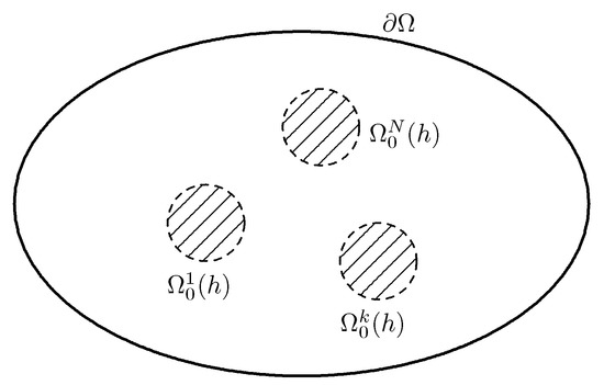
Figure 4. The structural condition (Z1) on the coefficient of intraspecific competition $h\left(x\right)$.

(Z1)

The open set ${\mathrm{\Omega }}_0\left(h\right)$ consists of a finite number of connected components with boundary of class $C^1$, say ${\mathrm{\Omega }}_0^k\left(h\right)$, $1\le k\le N$, which are bounded away from the boundary $\partial \mathrm{\Omega }$.

$${\mathrm{\Omega }}_0\left(h\right)=\bigcup _{k=1}^N{\mathrm{\Omega }}_0^k\left(h\right).$$

This structural condition is inspired by Ouyang [20], Theorem 2.

We consider the Dirichlet eigenvalue problem with indefinite weight function $m\left(x\right)$ in each connected component ${\mathrm{\Omega }}_0^k\left(h\right)$

$$\left\{\begin{array}{cc}-\Delta \psi \left(x\right)=\mu m\left(x\right)\psi \left(x\right)\hfill & \mathrm{in} {\mathrm{\Omega }}_0^k\left(h\right),\hfill \\ \psi \left(x^{\prime }\right)=0\hfill & \mathrm{on} \partial {\mathrm{\Omega }}_0^k\left(h\right),\hfill \end{array}\right.$$

(67)

where $\partial {\mathrm{\Omega }}_0^k\left(h\right)$ denotes the boundary of ${\mathrm{\Omega }}_0^k\left(h\right)$.

In this paper, we suppose that

(Z2)

Each set $\{x\in {\mathrm{\Omega }}_0^k\left(h\right):m\left(x\right)>0\}$ has positive measure for $1\le k\le N$,

and let ${\mu }_1\left({\mathrm{\Omega }}_0^k\left(h\right)\right)=\mathrm{the} first eigenvalue$ of the Dirichlet eigenvalue problem (67).

By applying Theorem 1 with

$$\begin{array}{cc}\hfill & \mathrm{\Omega }:={\mathrm{\Omega }}_0^k\left(h\right)for1\le k\le N,\hfill \\ \hfill & \left(M1\right):=\left(Z2\right),\hfill \end{array}$$

we obtain that the first eigenvalue ${\lambda }_1\left({\mathrm{\Omega }}_0^k\left(h\right)\right)$ is positive and algebraically simple:

$${\mu }_1\left({\mathrm{\Omega }}_0^k\left(h\right)\right)>0for1\le k\le N.$$

(68)

Moreover, by the Rayleigh principle ([18], Proposition 1.10; [21], Proposition 3.4) we know that the first eigenvalue ${\mu }_1\left({\mathrm{\Omega }}_0^k\left(h\right)\right)$ is given by the variational formula

$$\begin{array}{cc}\hfill & {\mu }_1\left({\mathrm{\Omega }}_0^k\left(h\right)\right)\hfill \\ \hfill & =inf\left\{\frac{{\int }_{{\mathrm{\Omega }}_0^k\left(h\right)}{|\nabla \psi \left(x\right)|}^{2}dx}{{\int }_{{\mathrm{\Omega }}_0^k\left(h\right)}m\left(x\right)\psi {\left(x\right)}^{2}dx}:\psi \in H_0^1\left({\mathrm{\Omega }}_0^k\left(h\right)\right),{\int }_{{\mathrm{\Omega }}_0^k\left(h\right)}m\left(x\right)\psi {\left(x\right)}^{2}dx>0\right\}.\hfill \end{array}$$

By virtue of assertion (68), we can associate with the open set ${\mathrm{\Omega }}_0\left(h\right)$ a positive number ${\mu }_1\left({\mathrm{\Omega }}_0\left(h\right)\right)$ as follows:

$${\mu }_1\left({\mathrm{\Omega }}_0\left(h\right)\right)=min\left\{{\mu }_1\left({\mathrm{\Omega }}_0^1\left(h\right)\right),{\mu }_1\left({\mathrm{\Omega }}_0^2\left(h\right)\right),\dots ,{\mu }_1\left({\mathrm{\Omega }}_0^N\left(h\right)\right)\right\}.$$

(69)

Remark 2.

It should be noticed (see Chavel [22] (p. 18, Corollary 1); López-Gómez [19] (Section 8.1)) that the value ${\mu }_1\left({\mathrm{\Omega }}_0\left(h\right)\right)$ tends to be smaller in situations where favorable and unfavorable habits are closely intermingled, and larger when the favorable region consists of a relatively small number of relatively large isolated components.

Now we can state our main result that is a generalization of Cantrell–Cosner [23] (Theorems 2.1 and 2.3), Hess–Kato [24] (Theorem 2) and Hess [25] (Theorem 27.1) to the case where the coefficient of intraspecific competition $h\left(x\right)$ may vanish in $\mathrm{\Omega }$ (see Figure 4 as above):

Theorem 6

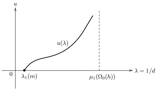
(the logistic Dirichlet case). Let $m\left(x\right)\in C^{\theta }\left(\overline{\mathrm{\Omega }}\right)$ for $0<\theta <1$. Suppose that condition (M1) and the structural conditions (Z1) and (Z2) are satisfied. Then the logistic Dirichlet problem (66) has a unique positive solution $u\left(\lambda \right)\in C^{2+\theta }\left(\overline{\mathrm{\Omega }}\right)$ for every $\lambda \in \left({\lambda }_1\left(m\right),{\mu }_1\left({\mathrm{\Omega }}_0\left(h\right)\right)\right)$. For any $\lambda \ge {\mu }_1\left({\mathrm{\Omega }}_0\left(h\right)\right)$, there exists no positive solution of the logistic Dirichlet problem (66). Moreover, we have the assertions (see Figure 5 below)

$$\begin{array}{cc}\hfill & \underset{\lambda \uparrow {\mu }_1\left({\mathrm{\Omega }}_0\left(h\right)\right)}{lim}{∥u\left(\lambda \right)∥}_{L^2\left(\mathrm{\Omega }\right)}=+\infty ,\hfill \\ \hfill & \underset{\lambda \downarrow {\lambda }_1\left(m\right)}{lim}{∥u\left(\lambda \right)∥}_{C^{2+\theta }\left(\overline{\mathrm{\Omega }}\right)}=0.\hfill \end{array}$$

Figure 5. A biological interpretation of Theorem 6 (the logistic Dirichlet case).

A biological interpretation of Theorem 6 (the logistic Dirichlet case) may be stated as follows (see Figure 5):

(i)

If the environment has a completely hostile boundary, then the models we consider predict persistence for a population if its diffusion rate d is below the critical value $1/{\lambda }_1\left(m\right)$ depending on the intrinsic growth rate $m\left(x\right)$ and if it is above the critical value $1/{\mu }_1\left({\mathrm{\Omega }}_0\left(h\right)\right)$ depending on the coefficient $h\left(x\right)$ describing the strength of the crowding effects.

(ii)

In a certain sense, the most favorable situations will occur if there is a relatively large favorable region (with good resources and without crowding effects) located some distance away from the boundary of $\mathrm{\Omega }$.

Some important remarks are in order:

Remark 3.

1°

Theorem 6 may be proved by using thesuper-sub-solution methodjust as in the proof of Fraile et al. [26] (Theorems 3.5 and 4.6), with a weaker assertion

$$\underset{\lambda \uparrow {\mu }_1\left({\mathrm{\Omega }}_0\left(h\right)\right)}{lim}{∥u\left(\lambda \right)∥}_{C\left(\overline{\mathrm{\Omega }}\right)}=+\infty .$$

2°

Theorem 6 asserts that the assertions hold true if the dimension n is greater than 2 ($n\ge 3$). It should be emphasized that an estimate of the growth rate of the total size ${\parallel u\left(\lambda \right)\parallel }_{L^1\left(\mathrm{\Omega }\right)}={\int }_{\mathrm{\Omega }}u\left(\lambda \right)dx$ of the positive steady states $u\left(\lambda \right)$ as $\lambda \uparrow {\mu }_1\left({\mathrm{\Omega }}_0\left(h\right)\right)$ is of crucial importance from the viewpoint of population dynamics.

3°

López-Gómez–Sabina de Lis [27] analyze the pointwise growth to infinity of positive solutions of the logistic Dirichlet problem in the case where $m\left(x\right)\equiv 1$ in Ω (see [27], Theorems 4.2 and 4.3). Furthermore, García-Melián et al. [28] study the pointwise behavior and the uniqueness of positive solutions of nonlinear elliptic boundary value problems of general sublinear type, and give the exact limiting profile of the positive solutions (see [28], Theorem 3.1, Corollary 3.3 and Theorem 6.4). Their numerical computations confirm and illuminate the above bifurcation diagram (Figure 5).

Remark 4.

Suppose that

$$h\left(x\right)>0on \overline{\mathrm{\Omega }},$$

(70)

and that the intrinsic growth rate $m\left(x\right)$ satisfies condition (M1). Then, by arguing as in the proof of Cantrell–Cosner [23] (Theorem 4.1) we can give an estimate of the decay rate of the total size of the positive steady states $u\left(\lambda \right)$:

$${\int }_{\mathrm{\Omega }}u\left(\lambda \right)dx\le \left(1-\frac{{\lambda }_1\left(m\right)}{\lambda }\right){\left|\mathrm{\Omega }\right|}^{2/3}\frac{{\left({\int }_{\mathrm{\Omega }}{m}^{+}{\left(x\right)}^{3}dx\right)}^{1/3}}{{min}_{x\in \overline{\mathrm{\Omega }}}h\left(x\right)}\mathit{for\; all} \lambda >{\lambda }_1\left(m\right).$$

Here $\left|\mathrm{\Omega }\right|$ is the volume of Ω and

$$m^{+}\left(x\right)=max\left\{m\left(x\right),0\right\}for x\in \mathrm{\Omega }.$$

Therefore, we find that the quantity

$${\left|\mathrm{\Omega }\right|}^{2/3}\frac{{\left({\int }_{\mathrm{\Omega }}{m}^{+}{\left(x\right)}^{3}dx\right)}^{1/3}}{{min}_{x\in \overline{\mathrm{\Omega }}}h\left(x\right)}$$

is the carrying capacity of the population.

5.3. Stability for Positive Solutions of Diffusive Logistic Dirichlet Problems

Secondly, by using Theorem 2 we can study the asymptotic stability properties for positive solutions of the logistic Dirichlet problem (66) (see [4] (Section 6)):

$$\left\{\begin{array}{cc}-\Delta u\left(x\right)=\lambda \left(m\left(x\right)-h\left(x\right)u\left(x\right)\right)u\left(x\right)\hfill & \mathrm{in} \mathrm{\Omega },\hfill \\ u\left(x^{\prime }\right)=0\hfill & \mathrm{on} \Gamma .\hfill \end{array}\right.$$

In this case, the dynamics of a population inhabiting a strongly heterogeneous environment is modeled by the semilinear parabolic initial boundary value problem Equation (65) with homogeneous Dirichlet condition

$$\left\{\begin{array}{cc}\frac{\partial w}{\partial t}(x,t)=d\Delta w(x,t)+\left(m\left(x\right)-h\left(x\right)w(x,t)\right)w(x,t)\hfill & \mathrm{in} \mathrm{\Omega }\times (0,\infty ),\hfill \\ w(x^{\prime },t)=0\hfill & \mathrm{on} \Gamma \times (0,\infty ),\hfill \\ w(x,0)=u_0\left(x\right)\hfill & \mathrm{in} \mathrm{\Omega }.\hfill \end{array}\right.$$

In order to study the semilinear parabolic problem (65), we may view it as generating a dynamical system. To do so, we consider the semilinear parabolic problem (65) with $d:=1/\lambda$:

$$\left\{\begin{array}{cc}\frac{\partial w}{\partial t}(x,t)=\frac{1}{\lambda }\Delta w(x,t)+\left(m\left(x\right)-h\left(x\right)w(x,t)\right)w(x,t)\hfill & \mathrm{in} \mathrm{\Omega }\times (0,\infty ),\hfill \\ w(x^{\prime },t)=0\hfill & \mathrm{on} \Gamma \times (0,\infty ),\hfill \\ w(x,0)=u_0\left(x\right)\hfill & \mathrm{in} \mathrm{\Omega }.\hfill \end{array}\right.$$

(71)

It is known (see [5] (p. 320, Theorems 5.2 and 5.3) and [29] (Proposition 3.4, Lemma 4.2, Theorem 4.5)) that the semilinear parabolic problem (71) admits a unique classical global solution $w(x,t;u_0)$ for each initial value $u_0\in C^{2+\theta }\left(\overline{\mathrm{\Omega }}\right)$ satisfying the compatibility conditions

$$\left\{\begin{array}{cc}{u}_0\left(x\right)\ge 0\hfill & \mathrm{in} \mathrm{\Omega },\hfill \\ u_0\left(x^{\prime }\right)=0\hfill & \mathrm{on} \Gamma .\hfill \end{array}\right.$$

(72)

A positive solution $w_0\left(x\right)$ of the logistic Dirichlet problem (66) is said to be globally asymptotically stable if we have the assertion

$$\underset{x\in \overline{\mathrm{\Omega }}}{max}\left|w(x,t;u_0)-w_0\left(x\right)\right|⟶0\mathrm{as} t\to \infty$$

for each non-trivial initial value $u_0\in C^{2+\theta }\left(\overline{\mathrm{\Omega }}\right)$ satisfying the compatibility conditions (72).

The next theorem, due to [16] (Theorem 1.3), describes the asymptotic stability properties for positive solutions of the logistic Dirichlet problem (66) (see Cantrell–Cosner [23] (Theorems 2.1 and 4.9), Fraile et al. [26] (Theorem 3.7)):

Theorem 7

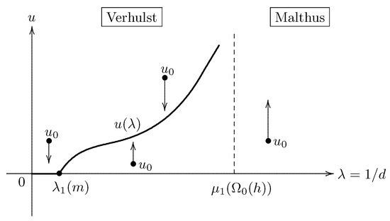
(the logistic Dirichlet case). Let $m\left(x\right)\in C^{\theta }\left(\overline{\mathrm{\Omega }}\right)$ for $0<\theta <1$. Suppose that condition (M1) and the structural conditions (Z1) and (Z2) are satisfied. Then we have the following three assertions (i)–(iii) (see Figure 6 below):

Figure 6. A biological interpretation of parts (i)–(iii) of Theorem 7 (the logistic Dirichlet case): Malthus versus Verhulst.

(i) 

The zero solution of the logistic Dirichet problem (66) is globally asymptotically stable if λ is so small that

$$0<\lambda <{\lambda }_1\left(m\right).$$

In this case, we can give an estimate of the decay rate of the total size of the population

$$\begin{array}{cc}\hfill & {\int }_{\mathrm{\Omega }}w(x,t;u_0)dx\hfill \\ \hfill & \le exp\left[-\left(\frac{1}{\lambda }-\frac{1}{{\lambda }_1\left(m\right)}\right){\lambda }_1\left(1\right)t\right]{\left|\mathrm{\Omega }\right|}^{1/2}{\left({\int }_{\mathrm{\Omega }}{u}_0{\left(x\right)}^{2}dx\right)}^{1/2}for all t>0.\hfill \end{array}$$

(73)

(ii) 

A positive solution $u\left(\lambda \right)$ of the logistic Dirichlet problem (66) is globally asymptotically stable for each λ satisfying the condition

$${\lambda }_1\left(m\right)<\lambda <{\mu }_1\left({\mathrm{\Omega }}_0\left(h\right)\right).$$

(iii) 

If λ is so large that

$$\lambda >{\mu }_1\left({\mathrm{\Omega }}_0\left(h\right)\right),$$

then we have the assertion

$$\underset{x\in \overline{\mathrm{\Omega }}}{max}\left|w(x,t;u_0)\right|⟶\infty as t\to \infty$$

(74)

for each non-trivial initial value $u_0\in C^{2+\theta }\left(\overline{\mathrm{\Omega }}\right)$ satisfying the compatibility conditions (72).

A biological interpretation of Theorem 7 (the logistic Dirichlet case) may be stated as follows (see Figure 6):

(i)

A population will grow exponentially until limited by lack of available resources if the diffusion rate $d=1/\lambda$ is below the critical value $1/{\mu }_1\left({\mathrm{\Omega }}_0\left(h\right)\right)$ (assertion (74) in part (iii)); this idea is generally credited to the English economist Thomas Robert Malthus (1776–1834).

(ii)

If the diffusion rate $d=1/\lambda$ is above the critical value $1/{\mu }_1\left({\mathrm{\Omega }}_0\left(h\right)\right)$, then the model obeys the logistic equation introduced by the Belgian mathematical biologist Pierre François Verhulst (1804–1849) around 1840 (the decay estimate (73) in part (i)).

5.4. Heuristic Approach to Diffusive Logistic Dirichlet Problems via the Semenov Approximation

This subsection is adapted from Taira [30]. For simplicity, we suppose that the coefficient of intraspecific competition $h\left(x\right)$ satisfies the condition (70)

$$h\left(x\right)>0\mathrm{on} \overline{\mathrm{\Omega }},$$

and further that the intrinsic growth rate $m\left(x\right)$ satisfies condition (M1). First, we rewrite the logistic Dirichlet problem (66) in the form

$$\left\{\begin{array}{cc}-\Delta u\left(x\right)=\lambda \left(m\left(x\right)-h\left(x\right)u\left(x\right)\right)u\left(x\right)\hfill & \mathrm{in} \mathrm{\Omega },\hfill \\ u\left(x\right)>0\hfill & \mathrm{in} \mathrm{\Omega },\hfill \\ u\left(x^{\prime }\right)=0\hfill & \mathrm{on} \Gamma .\hfill \end{array}\right.$$

Namely, we consider the logistic Dirichlet problem (66) as the Dirichlet eigenvalue problem with the weight $m\left(x\right)-h\left(x\right)u$.

However, Theorem 5 asserts that the first eigenvalue ${\lambda }_1\left(m\right)$ is the unique eigenvalue of the Dirichlet eigenvalue problem (62) corresponding to a positive eigenfunction ${\varphi }_1\left(x\right)$. Now we suppose that the solution u is of the form

$$u=C\left(\lambda \right){\varphi }_{1}for\lambda >{\lambda }_1\left(m\right),$$

where $C\left(\lambda \right)$ is a non-zero constant. Then we have the formulas

$$-\Delta u=-C\left(\lambda \right)\Delta {\varphi }_1=C\left(\lambda \right){\lambda }_1\left(m\right)m\left(x\right){\varphi }_1\mathrm{in} \mathrm{\Omega }$$

and

$$\lambda \left(m\left(x\right)-h\left(x\right)u\right)u=\lambda \left(m\left(x\right)-h\left(x\right)u\right)C\left(\lambda \right){\varphi }_1\mathrm{in} \mathrm{\Omega }.$$

This implies that

$$\lambda m\left(x\right)-\lambda h\left(x\right)u={\lambda }_1\left(m\right)m\left(x\right)\mathrm{in} \mathrm{\Omega },$$

so that

$$u=u\left(\lambda \right)={\displaystyle \frac{m\left(x\right)}{h\left(x\right)}}\left(1-\frac{{\lambda }_1\left(m\right)}{\lambda }\right)\mathrm{in} \mathrm{\Omega }.$$

Therefore, we obtain that the bifurcation solution curve $(\lambda ,u)$ of the logistic Dirichlet problem (66) is “formally” given by Formula (75), called the Semenov approximation in Chemistry ([31]),

$$u\left(\lambda \right)={\displaystyle \frac{m\left(x\right)}{h\left(x\right)}}\left(1-\frac{{\lambda }_1\left(m\right)}{\lambda }\right)for \lambda >{\lambda }_1\left(m\right).$$

(75)

In view of Formula (75) and Figure 7 below, we find that the quantity

$$\ell :={\displaystyle \frac{{max}_{\overline{\mathrm{\Omega }}}m}{{min}_{\overline{\mathrm{\Omega }}}h}}={\displaystyle \frac{{max}_{\overline{\mathrm{\Omega }}}{m}^{+}}{{min}_{\overline{\mathrm{\Omega }}}h}}$$

is the carrying capacity of the environment under condition (70).

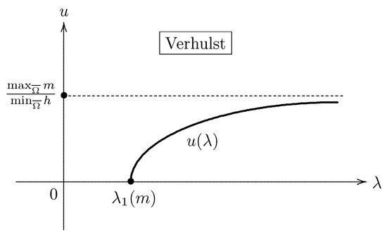
Figure 7. The formal positive solution curve $\left(\lambda ,u\left(\lambda \right)\right)$ for $\lambda >{\lambda }_1\left(m\right)$ under condition (70) (the logistic Dirichlet case).

5.5. Diffusive Logistic Neumann Problems

In this subsection, by using Theorem 2 we study the following semilinear parabolic initial boundary value problem with homogeneous Neumann condition of the form

$$\left\{\begin{array}{cc}\frac{\partial w}{\partial t}(x,t)=d\Delta w(x,t)+\left(m\left(x\right)-h\left(x\right)w(x,t)\right)w(x,t)\hfill & \mathrm{in} \mathrm{\Omega }\times (0,\infty ),\hfill \\ \frac{\partial w}{\partial \mathbf{n}}(x^{\prime },t)=0\hfill & \mathrm{on} \Gamma \times (0,\infty ),\hfill \\ w(x,0)=v_0\left(x\right)\hfill & \mathrm{in} \mathrm{\Omega },\hfill \end{array}\right.$$

(76)

where $\mathbf{n}$ is the unit outward normal to $\partial \mathrm{\Omega }$.

In order to study the semilinear initial boundary value problem (76), we may view it as generating a dynamical system. To do so, we consider the semilinear parabolic problem (76) with $d:=1/\lambda$:

$$\left\{\begin{array}{cc}\frac{\partial w}{\partial t}(x,t)=\frac{1}{\lambda }\Delta w(x,t)+\left(m\left(x\right)-h\left(x\right)w(x,t)\right)w(x,t)\hfill & \mathrm{in} \mathrm{\Omega }\times (0,\infty ),\hfill \\ \frac{\partial w}{\partial \mathbf{n}}(x^{\prime },t)=0\hfill & \mathrm{on} \Gamma \times (0,\infty ),\hfill \\ w(x,0)=u_0\left(x\right)\hfill & \mathrm{in} \mathrm{\Omega }.\hfill \end{array}\right.$$

(77)

It is known (see [5] (p. 320, Theorems 5.2 and 5.3) and [29] (Proposition 3.4, Lemma 4.2, Theorem 4.5)) that the semilinear parabolic problem (77) admits a unique classical global solution $w(x,t;v_0)$ for each initial value $v_0\in C^{2+\theta }\left(\overline{\mathrm{\Omega }}\right)$ satisfying the compatibility conditions

$$\left\{\begin{array}{cc}{v}_0\left(x\right)\ge 0\hfill & \mathrm{in} \mathrm{\Omega },\hfill \\ \frac{\partial v_0}{\partial \mathbf{n}}\left(x^{\prime }\right)=0\hfill & \mathrm{on} \Gamma .\hfill \end{array}\right.$$

(78)

The analysis of the semilinear parabolic problem (76) with homogeneous Neumann condition may be somewhat different since the operator $-\Delta$ with homogeneous Neumann condition has zero as an eigenvalue. However, the same general approach to the semilinear parabolic initial boundary value problem (65) with homogeneous Dirichlet condition can still be used (see Hess [25]).

First, we consider the linearized Neumann eigenvalue problem with an indefinite weight function $m\left(x\right)$ and a real parameter $\nu =1/d$:

$$\left\{\begin{array}{cc}-\Delta \psi \left(x\right)=\nu m\left(x\right)\psi \left(x\right)\hfill & \mathrm{in} \mathrm{\Omega },\hfill \\ \frac{\partial \psi }{\partial \mathbf{n}}\left(x^{\prime }\right)=0\hfill & \mathrm{on} \Gamma .\hfill \end{array}\right.$$

(79)

We discuss the structure of positive solutions of the eigenvalue problem (79) under the condition that:

(M2)

The intrinsic growth rate $m\left(x\right)$ belongs to the Hölder space $C^{\theta }\left(\overline{\mathrm{\Omega }}\right)$ for $0<\theta <1$ and it attains both positive and negative values in $\mathrm{\Omega }$.

If condition (M2) is satisfied, then the Neumann eigenvalue problem (79) admits a unique non-zero, eigenvalue ${\nu }_1\left(m\right)$ having a positive eigenfunction. More precisely, we have the following theorem (see Brown–Lin [32] (Theorem 3.13) and Senn–Hess [33] (Theorems 2 and 3)):

Theorem 8

(the Neumann case). If the intrinsic growth rate $m\left(x\right)$ satisfies condition (M2), then the Neumann eigenvalue problem (79) admits a uniquenon-zero, eigenvalue ${\nu }_1\left(m\right)$ having a positive eigenfunction. More precisely, we have the following three assertions (i)–(iii):

(i) 

If ${\int }_{\mathrm{\Omega }}m\left(x\right)dx<0$, then the smallest, non-zero eigenvalue ${\nu }_1\left(m\right)$ of the Neumann problem (79) is positive and simple, and its corresponding eigenfunction ${\psi }_1\left(x\right)\in C^{2+\theta }\left(\overline{\mathrm{\Omega }}\right)$ may be chosen to be strictly positive everywhere in Ω. Moreover, no other positive eigenvalues have positive eigenfunctions. The eigenvalue 0 is simple and has the positive eigenfunction ${\psi }_1\left(x\right)\equiv 1$ in Ω.

(ii) 

If ${\int }_{\mathrm{\Omega }}m\left(x\right)dx>0$, then the largest, non-zero eigenvalue ${\nu }_1\left(m\right)$ of the Neumann problem (79) is negative and simple, and its corresponding eigenfunction ${\psi }_1\left(x\right)\in C^{2+\theta }\left(\overline{\mathrm{\Omega }}\right)$ may be chosen to be strictly positive everywhere in Ω. Moreover, no other negative eigenvalues have positive eigenfunctions. The eigenvalue 0 is simple and has the positive eigenfunction ${\psi }_1\left(x\right)\equiv 1$ in Ω.

(iii) 

If ${\int }_{\mathrm{\Omega }}m\left(x\right)dx=0$, then the eigenvalue 0 of the Neumann problem (79) is the only eigenvalue having the positive eigenfunction ${\psi }_1\left(x\right)\equiv 1$ in Ω.

Next we study the following steady state problem with a parameter $d=1/\nu$:

$$\left\{\begin{array}{cc}-\Delta v\left(x\right)=\nu \left(m\left(x\right)-h\left(x\right)v\left(x\right)\right)v\left(x\right)\hfill & \mathrm{in} \mathrm{\Omega },\hfill \\ \frac{\partial v}{\partial \mathbf{n}}\left(x^{\prime }\right)=0\hfill & \mathrm{on} \Gamma .\hfill \end{array}\right.$$

(80)

This problem is the logistic Neumann problem.

Then we have the following generalization of Hess [25] (Example 28.6) to the case where the coefficient of intraspecific competition $h\left(x\right)$ may vanish in $\mathrm{\Omega }$ under the structural conditions (Z1) and (Z2) (see Fraile et al. [26] (Theorem 3.7), Senn [34] (Theorem 3.2)):

Theorem 9

(the logistic Neumann case). Suppose that condition (M2) and the structural conditions (Z1) and (Z2) are satisfied. Then we have the following two assertions (i) and (ii):

(i) 

If ${\int }_{\mathrm{\Omega }}m\left(x\right)dx<0$, the logistic Neumann problem (80) has a unique positive solution $v\left(\lambda \right)\in C^{2+\theta }\left(\overline{\mathrm{\Omega }}\right)$ for every $\lambda \in ({\nu }_1\left(m\right),{\mu }_1\left({\mathrm{\Omega }}_0\left(h\right)\right))$. For any $\lambda \ge {\mu }_1\left({\mathrm{\Omega }}_0\left(h\right)\right)$, there exists no positive solution of the semilinear problem (79). Moreover, we have the assertions

$$\begin{array}{cc}\hfill & \underset{\lambda \uparrow {\mu }_1\left({\mathrm{\Omega }}_0\left(h\right)\right)}{lim}{∥v\left(\lambda \right)∥}_{L^2\left(\mathrm{\Omega }\right)}=+\infty ,\hfill \\ \hfill & \underset{\lambda \downarrow {\nu }_1\left(m\right)}{lim}{∥v\left(\lambda \right)∥}_{C^{2+\theta }\left(\overline{\mathrm{\Omega }}\right)}=0.\hfill \end{array}$$

In a neighborhood of the point $(0,0)$ the solution set of the logistic Neumann problem (80) just consists of the two lines of trivial solutions (see Figure 8 below).

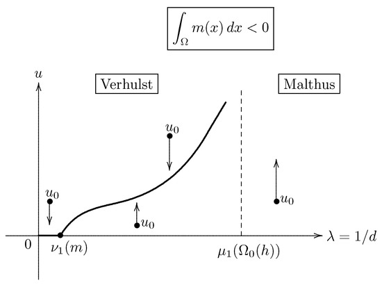Figure 8. A biological interpretation of part (i) of Theorem 9 in the case where ${\int }_{\mathrm{\Omega }}m\left(x\right)dx<0$: Malthus versus Verhulst.

(ii) 

${\int }_{\mathrm{\Omega }}m\left(x\right)dx\ge 0$, the logistic Neumann problem (80) has a unique positive solution $v\left(\lambda \right)\in C^{2+\theta }\left(\overline{\mathrm{\Omega }}\right)$ for every $\lambda \in (0,{\mu }_1\left({\mathrm{\Omega }}_0\left(h\right)\right))$. For each $\lambda \ge {\mu }_1\left({\mathrm{\Omega }}_0\left(h\right)\right)$, there exists no positive solution of the logistic Neumann problem (80). Moreover, we have the assertions

$$\begin{array}{cc}\hfill & \underset{\lambda \uparrow {\mu }_1\left({\mathrm{\Omega }}_0\left(h\right)\right)}{lim}{∥v\left(\lambda \right)∥}_{L^2\left(\mathrm{\Omega }\right)}=+\infty ,\hfill \\ \hfill & \underset{\lambda \downarrow 0}{lim}{∥v\left(\lambda \right)-c∥}_{C^{2+\theta }\left(\overline{\mathrm{\Omega }}\right)}=0,\hfill \end{array}$$

where

$$c=\left\{\begin{array}{cc}\frac{{\int }_{\mathrm{\Omega }}m\left(x\right)dx}{{\int }_{\mathrm{\Omega }}h\left(x\right)dx}\hfill & if{\int }_{\mathrm{\Omega }}m\left(x\right)dx>0,\hfill \\ 0\hfill & if{\int }_{\mathrm{\Omega }}m\left(x\right)dx=0.\hfill \end{array}\right.$$

Namely, if ${\int }_{\mathrm{\Omega }}m\left(x\right)dx>0$, there occurs a secondary bifurcation from the line $\left\{0\right\}\times \mathbf{R}$ of trivial solutions at the point $(0,c)$ (see Figure 9 below). If ${\int }_{\mathrm{\Omega }}m\left(x\right)dx=0$, there are two curves bifurcating at the point $(0,0)$; the line $\left\{0\right\}\times \mathbf{R}$ of trivial solutions and the curve $\{\left(\lambda ,u\left(\lambda \right)\right):\lambda >0\}$ (see Figure 10 below).

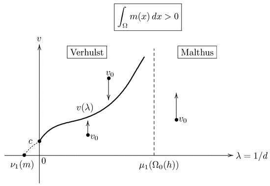Figure 9. A biological interpretation of part (ii) of Theorem 9 in the case where ${\int }_{\mathrm{\Omega }}m\left(x\right)dx>0$: Malthus versus Verhulst.

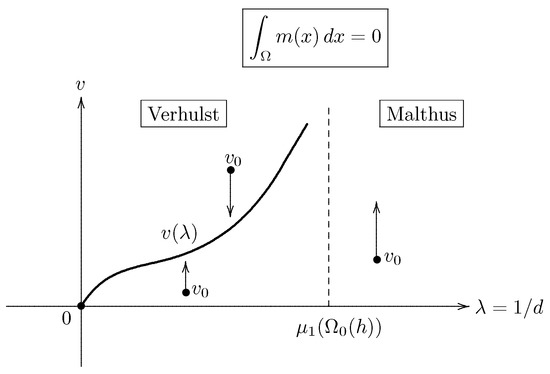Figure 10. A biological interpretation of part (ii) of Theorem 9 in the case where ${\int }_{\mathrm{\Omega }}m\left(x\right)dx=0$: Malthus versus Verhulst.

A biological interpretation of Theorem 9 (the logistic Neumann case) may be stated as follows (see Figure 8, Figure 9 and Figure 10):

(i)

When the environment has an impassable boundary and is on the average unfavorable, then high diffusion rates have the same effect as they always have when the boundary is deadly (cf. Figure 5).

(ii)

The behavior of solutions of the logistic Neumann problem (76) is similar to that of the problem (65) with homogeneous Dirichlet condition if ${\int }_{\mathrm{\Omega }}m\left(x\right)dx<0$. In fact, there is a positive eigenvalue with positive eigenfunction to act as a bifurcation point for positive steady states.

(iii)

If the boundary is impassable and the environment is on the average neutral or favorable, then the population can persist, no matter what its rate of diffusion.

(iv)

The behavior of solutions of the logistic Neumann problem (76) is similar to that of the problem (65) with homogeneous Dirichlet condition if ${\int }_{\mathrm{\Omega }}m\left(x\right)dx<0$. In fact, there is a positive eigenvalue with a positive eigenfunction to act as a bifurcation point for positive steady states (cf. Figure 6).

(v)

If ${\int }_{\mathrm{\Omega }}m\left(x\right)dx>0$, there occurs a secondary bifurcation from the line $\left\{0\right\}\times \mathbf{R}$ of trivial solutions.

(vi)

If ${\int }_{\mathrm{\Omega }}m\left(x\right)dx=0$, there are two curves bifurcating at the point $(0,0)$; the line $\left\{0\right\}\times \mathbf{R}$ of trivial solutions and the curve $\{\left(\lambda ,v\left(\lambda \right)\right):\lambda >0\}$.

More precisely, if the weight function $m\left(x\right)$ satisfies condition (M2), by using Cantrell–Cosner [23] (Theorem 4.1) and also Brown–Lin [32] (Theorem 3.13) we can prove the following stability theorem ([4], Theorem 1.5):

Theorem 10

(the logistic Neumann case). Suppose that condition (M2) and the structural conditions (Z1) and (Z2) are satisfied. Then we have the following two assertions (i) and (ii):

(i) 

If ${\int }_{\mathrm{\Omega }}m\left(x\right)dx<0$, then we have the following three assertions (a)–(c) (see Figure 11 below):

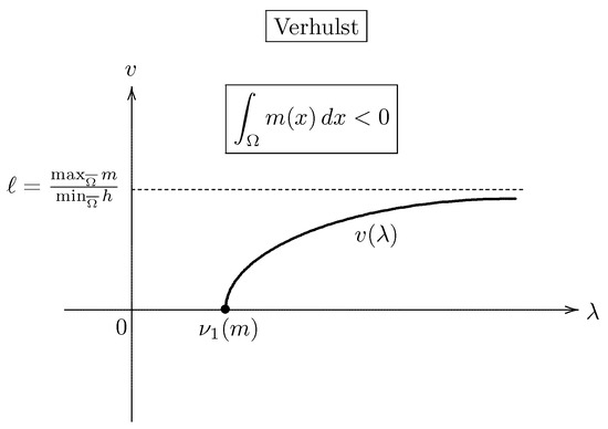Figure 11. A biological interpretation of part (i) of Theorem 10 in the case where ${\int }_{\mathrm{\Omega }}m\left(x\right)dx<0$ under condition (70) (Verhulst).

(a) 

The zero solution of the logistic Neumann problem (80) is globally asymptotically stableif λ is so small that $0<\lambda <{\nu }_1\left(m\right)$. In this case, we can obtain an estimate of the decay rate of the total size of the population

$$\begin{array}{cc}\hfill & {\int }_{\mathrm{\Omega }}w(x,t;v_0)dx\hfill \\ \hfill & \le exp\left[-\left(\frac{1}{\lambda }-\frac{1}{{\nu }_1\left(m\right)}\right){\nu }_1\left(1\right)t\right]{\left|\mathrm{\Omega }\right|}^{1/2}{\left({\int }_{\mathrm{\Omega }}{v}_0{\left(x\right)}^{2}dx\right)}^{1/2}for all t>0.\hfill \end{array}$$

(81)

(b) 

A positive solution $v\left(\lambda \right)$ of the logistic Neumann problem (80) is globally asymptotically stablefor each ${\nu }_1\left(m\right)<\lambda <{\mu }_1\left({\mathrm{\Omega }}_0\left(h\right)\right)$.

(c) 

If λ is so large that $\lambda >{\mu }_1\left({\mathrm{\Omega }}_0\left(h\right)\right)$, then we have the assertion

$$\underset{x\in \overline{\mathrm{\Omega }}}{max}\left|w(x,t;v_0)\right|⟶\infty as t\to \infty$$

(82)

for each non-trivial initial value $v_0\in C^{2+\theta }\left(\overline{\mathrm{\Omega }}\right)$ satisfying the compatibility conditions (78).

(ii) 

If ${\int }_{\mathrm{\Omega }}m\left(x\right)dx\ge 0$, then we have the following two assertions (d) and (e) (see Figure 12 and Figure 13 below):

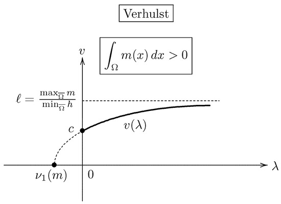Figure 12. A biological interpretation of Theorem 10 in the case where ${\int }_{\mathrm{\Omega }}m\left(x\right)dx>0$ under condition (70) (Verhulst).

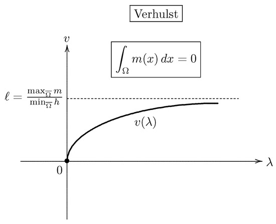Figure 13. A biological interpretation of Theorem 10 in the case where ${\int }_{\mathrm{\Omega }}m\left(x\right)dx=0$ under condition (70) (Verhulst).

(d) 

A positive solution $v\left(\lambda \right)$ of the logistic Neumann problem (80) is globally asymptotically stablefor each $0<\lambda <{\mu }_1\left({\mathrm{\Omega }}_0\left(h\right)\right)$.

(e) 

If λ is so large that $\lambda >{\mu }_1\left({\mathrm{\Omega }}_0\left(h\right)\right)$, then we have assertion (82) for each non-trivial initial value $v_0\in C^{2+\theta }\left(\overline{\mathrm{\Omega }}\right)$ satisfying the compatibility conditions (78).

Finally, we consider the case where the coefficient of intraspecific competition $h\left(x\right)$ satisfies the condition (70)

$$h\left(x\right)>0\mathrm{on} \overline{\mathrm{\Omega }}.$$

If the weight function $m\left(x\right)$ satisfies condition (M2), then, by combining Theorem 2 and Brown–Lin [32] (Theorem 3.13) we can characterize the carrying capacity of the environment (see [23] (Theorem 4.1); [4] (Theorem 1.6)):

Theorem 11

(the Neumann case). If conditions (M2) and (70) are satisfied, then we obtain that the quantity

$$\ell ={\displaystyle \frac{{max}_{\overline{\mathrm{\Omega }}}m}{{min}_{\overline{\mathrm{\Omega }}}h}}={\displaystyle \frac{{max}_{\overline{\mathrm{\Omega }}}{m}^{+}}{{min}_{\overline{\mathrm{\Omega }}}h}}$$

is the carrying capacity of the environment (see Figure 11, Figure 12 and Figure 13).

Remark 5.

Suppose that condition (70) is satisfied in the case ${\int }_{\mathrm{\Omega }}m\left(x\right)dx<0$. Then, by using the variational formula of Brown–Lin [32] (Theorem 3.13) we can prove the following decay estimate of the total size of the positive steady states $v\left(\lambda \right)$ (see Figure 11):

$$\begin{array}{cc}\hfill {\int }_{\mathrm{\Omega }}v\left(\lambda \right)dx& \le \left(1-\frac{{\nu }_1\left(m\right)}{\lambda }\right){\left|\mathrm{\Omega }\right|}^{2/3}\frac{{\left({\int }_{\mathrm{\Omega }}{m}^{+}{\left(x\right)}^{3}dx\right)}^{1/3}}{{min}_{x\in \overline{\mathrm{\Omega }}}h\left(x\right)}\hfill \\ \hfill & forall \lambda >{\nu }_1\left(m\right).\hfill \end{array}$$

This proves that the quantity

$${\left|\mathrm{\Omega }\right|}^{2/3}\frac{{\left({\int }_{\mathrm{\Omega }}{m}^{+}{\left(x\right)}^{3}dx\right)}^{1/3}}{{min}_{x\in \overline{\mathrm{\Omega }}}h\left(x\right)}$$

is the carrying capacity of the population, just as in the Dirichlet case (see Remark 4).

Appendix A.1. Function Spaces for Equations of Parabolic Type

In this subsection we introduce function spaces associated with the linear initial boundary value problems (A1) and (A2).

We consider $\sigma$-Hölder continuous functions on $\overline{\mathrm{\Omega }}\times [0,\infty )$ where we use the metric

$$d\left((x,t),(x^{\prime },t^{\prime })\right)={\left(|x-x^{\prime }{|}^2+|t-t^{\prime }|\right)}^{1/2}$$

for the computation of the Hölder constant (see [6] (Chapter 3, Section 2)).

(I) The space $C^{\sigma ,\sigma /2}\left(\overline{Q_T}\right)$ for $0<\sigma <1$: First, we let

$$\begin{array}{cc}\hfill C^{\sigma ,\sigma /2}\left(\overline{Q_T}\right):=& \mathrm{t}\mathrm{h}\mathrm{e} \mathrm{s}\mathrm{p}\mathrm{a}\mathrm{c}\mathrm{e} \mathrm{o}\mathrm{f} \mathrm{c}\mathrm{o}\mathrm{n}\mathrm{t}\mathrm{i}\mathrm{n}\mathrm{u}\mathrm{o}\mathrm{u}\mathrm{s} \mathrm{f}\mathrm{u}\mathrm{n}\mathrm{c}\mathrm{t}\mathrm{i}\mathrm{o}\mathrm{n}\mathrm{s} u(x,t)\in C\left(\overline{Q_T}\right)\hfill \\ \hfill & \mathrm{t}\mathrm{h}\mathrm{a}\mathrm{t} \mathrm{a}\mathrm{r}\mathrm{e}\sigma \text{-}\mathrm{H}\mathrm{ö}\mathrm{l}\mathrm{d}\mathrm{e}\mathrm{r} \mathrm{c}\mathrm{o}\mathrm{n}\mathrm{t}\mathrm{i}\mathrm{n}\mathrm{u}\mathrm{o}\mathrm{u}\mathrm{s} \mathrm{w}\mathrm{i}\mathrm{t}\mathrm{h} \mathrm{r}\mathrm{e}\mathrm{s}\mathrm{p}\mathrm{e}\mathrm{c}\mathrm{t} \mathrm{t}\mathrm{o} x\hfill \\ \hfill & \mathrm{a}\mathrm{n}\mathrm{d} \sigma /2\text{-}\mathrm{H}\mathrm{ö}\mathrm{l}\mathrm{d}\mathrm{e}\mathrm{r} \mathrm{c}\mathrm{o}\mathrm{n}\mathrm{t}\mathrm{i}\mathrm{n}\mathrm{u}\mathrm{o}\mathrm{u}\mathrm{s} \mathrm{w}\mathrm{i}\mathrm{t}\mathrm{h} \mathrm{r}\mathrm{e}\mathrm{s}\mathrm{p}\mathrm{e}\mathrm{c}\mathrm{t} \mathrm{t}\mathrm{o} t.\hfill \end{array}$$

We introduce the following two seminorms:

$$\begin{array}{cc}\hfill & •{⟨u⟩}_{x,Q_T}^{\left(\sigma \right)}=\underset{\begin{array}{c}(x,t)\in Q_T,\\ (x^{\prime },t)\in Q_T\end{array}}{sup}\frac{\left|u(x,t)-u(x^{\prime },t)\right|}{|x-x^{\prime }{|}^{\sigma }},\hfill \\ \hfill & •{⟨u⟩}_{t,Q_T}^{(\sigma /2)}=\underset{\begin{array}{c}(x,t)\in Q_T,\\ (x,t^{\prime })\in Q_T\end{array}}{sup}\frac{\left|u(x,t)-u(x,t^{\prime })\right|}{|t-t^{\prime }{|}^{\sigma /2}},\hfill \end{array}$$

and the norm

$${∥u∥}_{Q_T}^{\left(\sigma \right)}=\underset{(x,t)\in \overline{Q_T}}{max}\left|u(x,t)\right|+{⟨u⟩}_{x,Q_T}^{\left(\sigma \right)}+{⟨u⟩}_{t,Q_T}^{(\sigma /2)}.$$

We remark that:

(1)

$u\in C\left(\left[0,T\right],C^{\sigma }\left(\overline{\mathrm{\Omega }}\right)\right)⟹{⟨u⟩}_{x,Q_T}^{\left(\sigma \right)}<\infty$.

(2)

$u\in C^{\sigma /2}\left(\left[0,T\right],C\left(\overline{\mathrm{\Omega }}\right)\right)⟹{⟨u⟩}_{t,Q_T}^{(\sigma /2)}<\infty$.

(II) The space $C^{1+\sigma ,(1+\sigma )/2}\left(\overline{Q_T}\right)$ for $0<\sigma <1$: Secondly, we let

$$\begin{array}{cc}\hfill C^{1+\sigma ,(1+\sigma )/2}\left(\overline{Q_T}\right):=& \mathrm{t}\mathrm{h}\mathrm{e} \mathrm{s}\mathrm{p}\mathrm{a}\mathrm{c}\mathrm{e} \mathrm{o}\mathrm{f} \mathrm{c}\mathrm{o}\mathrm{n}\mathrm{t}\mathrm{i}\mathrm{n}\mathrm{u}\mathrm{o}\mathrm{u}\mathrm{s}\mathrm{l}\mathrm{y} \mathrm{d}\mathrm{i}\mathrm{f}\mathrm{f}\mathrm{e}\mathrm{r}\mathrm{e}\mathrm{n}\mathrm{t}\mathrm{i}\mathrm{a}\mathrm{b}\mathrm{l}\mathrm{e} \mathrm{f}\mathrm{u}\mathrm{n}\mathrm{c}\mathrm{t}\mathrm{i}\mathrm{o}\mathrm{n}\mathrm{s}\hfill \\ \hfill & u(x,t)\in C^{1,0}\left(\overline{Q_T}\right) \mathrm{w}\mathrm{i}\mathrm{t}\mathrm{h} \mathrm{r}\mathrm{e}\mathrm{s}\mathrm{p}\mathrm{e}\mathrm{c}\mathrm{t} \mathrm{t}\mathrm{o} x \mathrm{s}\mathrm{u}\mathrm{c}\mathrm{h} \mathrm{t}\mathrm{h}\mathrm{a}\mathrm{t} \hfill \\ \hfill & {\partial }_{x}u(x,t) \mathrm{a}\mathrm{r}\mathrm{e} \sigma \text{-}\mathrm{H}\mathrm{ö}\mathrm{l}\mathrm{d}\mathrm{e}\mathrm{r} \mathrm{c}\mathrm{o}\mathrm{n}\mathrm{t}\mathrm{i}\mathrm{n}\mathrm{u}\mathrm{o}\mathrm{u}\mathrm{s} \mathrm{w}\mathrm{i}\mathrm{t}\mathrm{h} \mathrm{r}\mathrm{e}\mathrm{s}\mathrm{p}\mathrm{e}\mathrm{c}\mathrm{t} \mathrm{t}\mathrm{o} x \mathrm{a}\mathrm{n}\mathrm{d} \hfill \\ \hfill & \sigma /2\text{-}\mathrm{H}\mathrm{ö}\mathrm{l}\mathrm{d}\mathrm{e}\mathrm{r} \mathrm{c}\mathrm{o}\mathrm{n}\mathrm{t}\mathrm{i}\mathrm{n}\mathrm{u}\mathrm{o}\mathrm{u}\mathrm{s} \mathrm{w}\mathrm{i}\mathrm{t}\mathrm{h} \mathrm{r}\mathrm{e}\mathrm{s}\mathrm{p}\mathrm{e}\mathrm{c}\mathrm{t} \mathrm{t}\mathrm{o} t \mathrm{a}\mathrm{n}\mathrm{d} \mathrm{f}\mathrm{u}\mathrm{r}\mathrm{t}\mathrm{h}\mathrm{e}\mathrm{r} \mathrm{t}\mathrm{h}\mathrm{a}\mathrm{t}\hfill \\ \hfill & u(x,t)is(1+\sigma )/2\text{-}\mathrm{H}\mathrm{ö}\mathrm{l}\mathrm{d}\mathrm{e}\mathrm{r} \mathrm{c}\mathrm{o}\mathrm{n}\mathrm{t}\mathrm{i}\mathrm{n}\mathrm{u}\mathrm{o}\mathrm{u}\mathrm{s} \mathrm{w}\mathrm{i}\mathrm{t}\mathrm{h} \mathrm{r}\mathrm{e}\mathrm{s}\mathrm{p}\mathrm{e}\mathrm{c}\mathrm{t} \mathrm{t}\mathrm{o} t.\hfill \end{array}$$

We introduce the following three seminorms:

$$\begin{array}{cc}\hfill & •{⟨{\partial }_{x}u⟩}_{x,Q_T}^{\left(\sigma \right)}=\underset{\begin{array}{c}(x,t)\in Q_T,\\ (x^{\prime },t)\in Q_T\end{array}}{sup}\frac{\left|{\partial }_{x}u(x,t)-{\partial }_{x}u(x^{\prime },t)\right|}{|x-x^{\prime }{|}^{\sigma }},\hfill \\ \hfill & •{⟨u⟩}_{t,Q_T}^{\left(\right(\sigma +1)/2)}=\underset{\begin{array}{c}(x,t)\in Q_T,\\ (x,t^{\prime })\in Q_T\end{array}}{sup}\frac{\left|u(x,t)-u(x,t^{\prime })\right|}{|t-t^{\prime }{|}^{(1+\sigma )/2}},\hfill \\ \hfill & •{⟨{\partial }_{x}u⟩}_{t,Q_T}^{(\sigma /2)}=\underset{\begin{array}{c}(x,t)\in Q_T,\\ (x,t^{\prime })\in Q_T\end{array}}{sup}\frac{\left|{\partial }_{x}u(x,t)-{\partial }_{x}u(x,t^{\prime })\right|}{|t-t^{\prime }{|}^{\sigma /2}},\hfill \end{array}$$

and the norm

$$\begin{array}{cc}\hfill {∥u∥}_{Q_T}^{(1+\sigma )}& =\underset{(x,t)\in \overline{Q_T}}{max}\left|u(x,t)\right|+\underset{(x,t)\in \overline{Q_T}}{max}\left|{\partial }_{x}u(x,t)\right|\hfill \\ \hfill & +{⟨{\partial }_{x}u⟩}_{x,Q_T}^{\left(\sigma \right)}+{⟨u⟩}_{t,Q_T}^{\left(\right(\sigma +1)/2)}+{⟨{\partial }_{x}u⟩}_{t,Q_T}^{(\sigma /2)}.\hfill \end{array}$$

We remark that:

(1)

$u\in C\left(\left[0,T\right],C^{1+\sigma }\left(\overline{\mathrm{\Omega }}\right)\right)⟹{⟨{\partial }_{x}u⟩}_{x,Q_T}^{\left(\sigma \right)}<\infty$.

(2)

$u\in C^{\sigma /2}\left(\left[0,T\right],C^1\left(\overline{\mathrm{\Omega }}\right)\right)⟹{⟨{\partial }_{x}u⟩}_{t,Q_T}^{(\sigma /2)}<\infty$.

(III) The space $C^{2+\sigma ,1+\sigma /2}\left(\overline{Q_T}\right)$ for $0<\sigma <1$: Thirdly, we let

$$\begin{array}{cc}\hfill C^{2+\sigma ,1+\sigma /2}\left(\overline{Q_T}\right):=& \mathrm{t}\mathrm{h}\mathrm{e} \mathrm{s}\mathrm{p}\mathrm{a}\mathrm{c}\mathrm{e} \mathrm{o}\mathrm{f} \mathrm{c}\mathrm{o}\mathrm{n}\mathrm{t}\mathrm{i}\mathrm{n}\mathrm{u}\mathrm{o}\mathrm{u}\mathrm{s}\mathrm{l}\mathrm{y} \mathrm{d}\mathrm{i}\mathrm{f}\mathrm{f}\mathrm{e}\mathrm{r}\mathrm{e}\mathrm{n}\mathrm{t}\mathrm{i}\mathrm{a}\mathrm{b}\mathrm{l}\mathrm{e} \mathrm{f}\mathrm{u}\mathrm{n}\mathrm{c}\mathrm{t}\mathrm{i}\mathrm{o}\mathrm{n}\mathrm{s}\hfill \\ \hfill & u(x,t)\in C^{2,1}\left(\overline{Q_T}\right) \mathrm{t}\mathrm{w}\mathrm{i}\mathrm{c}\mathrm{e} \mathrm{w}\mathrm{i}\mathrm{t}\mathrm{h} \mathrm{r}\mathrm{e}\mathrm{s}\mathrm{p}\mathrm{e}\mathrm{c}\mathrm{t} \mathrm{t}\mathrm{o} x \mathrm{a}\mathrm{n}\mathrm{d} \mathrm{o}\mathrm{n}\mathrm{c}\mathrm{e}\hfill \\ \hfill & \mathrm{w}\mathrm{i}\mathrm{t}\mathrm{h} \mathrm{r}\mathrm{e}\mathrm{s}\mathrm{p}\mathrm{e}\mathrm{c}\mathrm{t} \mathrm{t}\mathrm{o} t \mathrm{s}\mathrm{u}\mathrm{c}\mathrm{h} \mathrm{t}\mathrm{h}\mathrm{a}\mathrm{t} {\partial }_{x}u(x,t) \mathrm{a}\mathrm{r}\mathrm{e} (1+\sigma )/2-\mathrm{H}\mathrm{ö}\mathrm{l}\mathrm{d}\mathrm{e}\mathrm{r}\hfill \\ \hfill & \mathrm{c}\mathrm{o}\mathrm{n}\mathrm{t}\mathrm{i}\mathrm{n}\mathrm{u}\mathrm{o}\mathrm{u}\mathrm{s} \mathrm{w}\mathrm{i}\mathrm{t}\mathrm{h} \mathrm{r}\mathrm{e}\mathrm{s}\mathrm{p}\mathrm{e}\mathrm{c}\mathrm{t} \mathrm{t}\mathrm{o} t ,\mathrm{t}\mathrm{h}\mathrm{a}\mathrm{t} {\partial }_{t}u(x,t) \mathrm{i}\mathrm{s} \sigma -\mathrm{H}\mathrm{ö}\mathrm{l}\mathrm{d}\mathrm{e}\mathrm{r}\hfill \\ \hfill & \mathrm{c}\mathrm{o}\mathrm{n}\mathrm{t}\mathrm{i}\mathrm{n}\mathrm{u}\mathrm{o}\mathrm{u}\mathrm{s} \mathrm{w}\mathrm{i}\mathrm{t}\mathrm{h} \mathrm{r}\mathrm{e}\mathrm{s}\mathrm{p}\mathrm{e}\mathrm{c}\mathrm{t} \mathrm{t}\mathrm{o} x \mathrm{a}\mathrm{n}\mathrm{d} \sigma /2-\mathrm{H}\mathrm{ö}\mathrm{l}\mathrm{d}\mathrm{e}\mathrm{r} \mathrm{c}\mathrm{o}\mathrm{n}\mathrm{t}\mathrm{i}\mathrm{n}\mathrm{u}\mathrm{o}\mathrm{u}\mathrm{s}\hfill \\ \hfill & \mathrm{w}\mathrm{i}\mathrm{t}\mathrm{h} \mathrm{r}\mathrm{e}\mathrm{s}\mathrm{p}\mathrm{e}\mathrm{c}\mathrm{t} \mathrm{t}\mathrm{o} t \mathrm{a}\mathrm{n}\mathrm{d} \mathrm{f}\mathrm{u}\mathrm{r}\mathrm{t}\mathrm{h}\mathrm{e}\mathrm{r} \mathrm{t}\mathrm{h}\mathrm{a}\mathrm{t}{\partial }_x^{2}u(x,t) \mathrm{a}\mathrm{r}\mathrm{e} \sigma -\mathrm{H}\mathrm{ö}\mathrm{l}\mathrm{d}\mathrm{e}\mathrm{r}\hfill \\ \hfill & \mathrm{c}\mathrm{o}\mathrm{n}\mathrm{t}\mathrm{i}\mathrm{n}\mathrm{u}\mathrm{o}\mathrm{u}\mathrm{s} \mathrm{w}\mathrm{i}\mathrm{t}\mathrm{h} \mathrm{r}\mathrm{e}\mathrm{s}\mathrm{p}\mathrm{e}\mathrm{c}\mathrm{t} \mathrm{t}\mathrm{o} x \mathrm{a}\mathrm{n}\mathrm{d} \sigma /2-\mathrm{H}\mathrm{ö}\mathrm{l}\mathrm{d}\mathrm{e}\mathrm{r} \mathrm{c}\mathrm{o}\mathrm{n}\mathrm{t}\mathrm{i}\mathrm{n}\mathrm{u}\mathrm{o}\mathrm{u}\mathrm{s}\hfill \\ \hfill & \mathrm{w}\mathrm{i}\mathrm{t}\mathrm{h} \mathrm{r}\mathrm{e}\mathrm{s}\mathrm{p}\mathrm{e}\mathrm{c}\mathrm{t} \mathrm{t}\mathrm{o} t.\hfill \end{array}$$

We introduce the following five seminorms:

$$\begin{array}{cc}\hfill & •{⟨{\partial }_{t}u⟩}_{x,Q_T}^{\left(\sigma \right)}=\underset{\begin{array}{c}(x,t)\in Q_T,\\ (x^{\prime },t)\in Q_T\end{array}}{sup}\frac{\left|{\partial }_{t}u(x,t)-{\partial }_{t}u(x^{\prime },t)\right|}{|x-x^{\prime }{|}^{\sigma }},\hfill \\ \hfill & •{⟨{\partial }_x^{2}u⟩}_{x,Q_T}^{\left(\sigma \right)}=\underset{\begin{array}{c}(x,t)\in Q_T,\\ (x^{\prime },t)\in Q_T\end{array}}{sup}\frac{\left|{\partial }_x^{2}u(x,t)-{\partial }_x^{2}u(x^{\prime },t)\right|}{|x-x^{\prime }{|}^{\sigma }},\hfill \\ \hfill & •{⟨{\partial }_{t}u⟩}_{t,Q_T}^{(\sigma /2)}=\underset{\begin{array}{c}(x,t)\in Q_T,\\ (x,t^{\prime })\in Q_T\end{array}}{sup}\frac{\left|{\partial }_{t}u(x,t)-{\partial }_{t}u(x,t^{\prime })\right|}{|t-t^{\prime }{|}^{\sigma /2}},\hfill \\ \hfill & •{⟨{\partial }_{x}u⟩}_{t,Q_T}^{\left(\right(1+\sigma )/2)}=\underset{\begin{array}{c}(x,t)\in Q_T,\\ (x,t^{\prime })\in Q_T\end{array}}{sup}\frac{\left|{\partial }_{x}u(x,t)-{\partial }_{x}u(x,t^{\prime })\right|}{|t-t^{\prime }{|}^{(1+\sigma )/2}},\hfill \\ \hfill & •{⟨{\partial }_x^{2}u⟩}_{t,Q_T}^{(\sigma /2)}=\underset{\begin{array}{c}(x,t)\in Q_T,\\ (x,t^{\prime })\in Q_T\end{array}}{sup}\frac{\left|{\partial }_x^{2}u(x,t)-{\partial }_x^{2}u(x,t^{\prime })\right|}{|t-t^{\prime }{|}^{\sigma /2}},\hfill \end{array}$$

and the norm

$$\begin{array}{cc}\hfill & {∥u∥}_{Q_T}^{(2+\sigma )}\hfill \\ \hfill & =\underset{(x,t)\in \overline{Q_T}}{max}\left|u(x,t)\right|+\underset{(x,t)\in \overline{Q_T}}{max}\left|{\partial }_{x}u(x,t)\right|+\underset{(x,t)\in \overline{Q_T}}{max}\left|{\partial }_{t}u(x,t)\right|+\underset{(x,t)\in \overline{Q_T}}{max}\left|{\partial }_x^{2}u(x,t)\right|\hfill \\ \hfill & +{⟨{\partial }_{t}u⟩}_{x,Q_T}^{\left(\sigma \right)}+{⟨{\partial }_x^{2}u⟩}_{x,Q_T}^{\left(\sigma \right)}+{⟨{\partial }_{t}u⟩}_{t,Q_T}^{(\sigma /2)}+{⟨{\partial }_{x}u⟩}_{t,Q_T}^{\left(\right(1+\sigma )/2)}+{⟨{\partial }_x^{2}u⟩}_{t,Q_T}^{(\sigma /2)}.\hfill \end{array}$$

We remark that:

(1)

$u\in C\left(\left[0,T\right],C^{2+\sigma }\left(\overline{\mathrm{\Omega }}\right)\right)⟹{⟨{\partial }_x^{2}u⟩}_{x,Q_T}^{\left(\sigma \right)}<\infty$.

(2)

$u\in C^{\sigma /2}\left(\left[0,T\right],C^2\left(\overline{\mathrm{\Omega }}\right)\right)⟹{⟨{\partial }_x^{2}u⟩}_{t,Q_T}^{(\sigma /2)}<\infty$.

(IV) The space $C^{2+\sigma ,1+\sigma /2}\left(\overline{{\Gamma }_T}\right)$ for $0<\sigma <1$: Finally, we let

$$\begin{array}{cc}\hfill C^{2+\sigma ,1+\sigma /2}\left(\overline{{\Gamma }_T}\right):=& \mathrm{t}\mathrm{h}\mathrm{e} \mathrm{s}\mathrm{p}\mathrm{a}\mathrm{c}\mathrm{e} \mathrm{o}\mathrm{f} \mathrm{f}\mathrm{u}\mathrm{n}\mathrm{c}\mathrm{t}\mathrm{i}\mathrm{o}\mathrm{n}\mathrm{s} \psi \mathrm{d}\mathrm{e}\mathrm{f}\mathrm{i}\mathrm{n}\mathrm{e}\mathrm{d} \mathrm{o}\mathrm{n} \overline{{\Gamma }_T} \mathrm{s}\mathrm{u}\mathrm{c}\mathrm{h}\hfill \\ \hfill & \mathrm{t}\mathrm{h}\mathrm{a}\mathrm{t} \mathrm{t}\mathrm{h}\mathrm{e}\mathrm{r}\mathrm{e} \mathrm{e}\mathrm{x}\mathrm{i}\mathrm{s}\mathrm{t} \mathrm{f}\mathrm{u}\mathrm{n}\mathrm{c}\mathrm{t}\mathrm{i}\mathrm{o}\mathrm{n}\mathrm{s} \Psi \in C^{2+\sigma ,1+\sigma /2}\left(\overline{Q_T}\right)\hfill \\ \hfill & \mathrm{w}\mathrm{h}\mathrm{i}\mathrm{c}\mathrm{h} \mathrm{c}\mathrm{o}\mathrm{i}\mathrm{n}\mathrm{c}\mathrm{i}\mathrm{d}\mathrm{e} \mathrm{w}\mathrm{i}\mathrm{t}\mathrm{h} \psi \mathrm{o}\mathrm{n} \overline{{\Gamma }_T}.\hfill \end{array}$$

We equip the Hölder space $C^{2+\sigma ,1+\sigma /2}\left(\overline{{\Gamma }_T}\right)$ with the norm

$${∥\psi ∥}_{{\Gamma }_T}^{(2+\sigma )}=inf{∥\Psi ∥}_{Q_T}^{(2+\sigma )},$$

where the infimum is taken over all such $\Psi$.

Appendix A.2. Unique Solvability Theorems for Linear Initial Boundary Value Problems of Parabolic Type

In this subsection we formulate unique solvability theorems for problems (A1) and (A2) in the framework of Hölder spaces.

(I) The Dirichlet case: Let $0<\mu <1$ and $T>0$. We suppose that

$$\left\{\begin{array}{c}f\in C^{\mu ,\mu /2}\left(\overline{Q_T}\right),\hfill \\ \phi \in C^{\mu +2,\mu /2+1}\left(\overline{{\Gamma }_T}\right),\hfill \\ u_0\in C^{\mu +2}\left(\overline{\mathrm{\Omega }}\right).\hfill \end{array}\right.$$

Then we have the following theorem ([5] (Chapter IV, Theorem 5.2)):

Theorem A1

(the Dirichlet case). Suppose that the following compatibility condition is satisfied:

$$\begin{array}{cc}\hfill & \phi (x^{\prime },0)=u_0\left(x^{\prime }\right)for all x^{\prime }\in \Gamma ,\hfill \\ \hfill & \Delta u_0\left(x^{\prime }\right)+f(x^{\prime },0)=\frac{\partial \phi }{\partial t}(x^{\prime },0)for all x^{\prime }\in \Gamma .\hfill \end{array}$$

Then the linear initial boundary value problem (A1) has a unique solution

$$u(x,t)\in C^{\mu +2,\mu /2+1}\left(\overline{\mathrm{\Omega }}\times \left[0,T\right]\right).$$

Moreover, we have the a priori estimate

$${∥u∥}_{Q_T}^{(\mu +2)}\le C_1\left({∥f∥}_{Q_T}^{\left(\mu \right)}+{\left|\phi \right|}_{{\Gamma }_T}^{(\mu +2)}+{∥u_0∥}_{\mathrm{\Omega }}^{(\mu +2)}\right),$$

(A3)

with a constant $C_1=C_1\left(T\right)>0$.

(II) The regular oblique derivative case: Let $0<\mu <1$ and $T>0$. We suppose that

$$\left\{\begin{array}{c}f\in C^{\mu ,\mu /2}\left(\overline{Q_T}\right),\hfill \\ \phi \in C^{\mu +1,(\mu +1)/2}\left(\overline{{\Gamma }_T}\right),\hfill \\ u_0\in C^{\mu +2}\left(\overline{\mathrm{\Omega }}\right).\hfill \end{array}\right.$$

Then we have the following theorem ([5] (Chapter IV, Theorem 5.3)):

Theorem A2

(the regular oblique derivative case). Suppose that the following compatibility condition is satisfied:

$$\frac{\partial u}{\partial \beta }\left(x^{\prime }\right)+b_0\left(x^{\prime }\right)u_0\left(x^{\prime }\right)=\phi (x^{\prime },0)\mathit{for\; all} x^{\prime }\in \Gamma .$$

Then the linear initial boundary value problem (A2) has a unique solution

$$u(x,t)\in C^{\mu +2,\mu /2+1}\left(\overline{\mathrm{\Omega }}\times \left[0,T\right]\right).$$

Moreover, we have the a priori estimate

$${∥u∥}_{Q_T}^{(\mu +2)}\le C_2\left({∥f∥}_{Q_T}^{\left(\mu \right)}+{\left|\phi \right|}_{{\Gamma }_T}^{(\mu +1)}+{∥u_0∥}_{\mathrm{\Omega }}^{(\mu +2)}\right),$$

(A4)

with a constant $C_2=C_2\left(T\right)>0$.

References

- Taira, K. Analytic Semigroups and Semilinear Initial-Boundary Value Problems, 2nd ed.; London Mathematical Society Lecture Note Series; Cambridge University Press: Cambridge, UK, 2016; Volume 434. [Google Scholar]
- Lions, J.-L.; Peetre, J. Sur une classe d’espaces d’interpolation. Inst. Hautes Études Sci. Publ. Math. 1964, 19, 5–68. [Google Scholar] [CrossRef]
- Redlinger, R. Über die C2-Kompaktheit der Bahn von Lösungen semilinearer parabolischer Systeme. Proc. R. Soc. Edinb. Sect. A Math. 1982, 93, 99–103. [Google Scholar] [CrossRef]
- Taira, K. A mathematical study of diffusive logistic equations with mixed type boundary conditions. Discret. Contin. Dyn. Syst. S 2021. Available online: https://www.aimsciences.org/article/doi/10.3934/dcdss.2021166 (accessed on 1 December 2021). [CrossRef]
- Ladyženskaja, O.A.; Solonnikov, V.A.; Ural’ceva, N.N. Linear and Quasilinear Equations of Parabolic Type; Smith, S., Translator; Translated from the Russian, Translations of Mathematical Monographs; American Mathematical Society: Providence, RI, USA, 1968; Volume 23. [Google Scholar]
- Friedman, A. Partial Differential Equations of Parabolic Type; Dover Publications Inc.: Mineola, NY, USA, 2008. [Google Scholar]
- Henry, D. Geometric Theory of Semilinear Parabolic Equations; Lecture Notes in Mathematics No. 840; Springer: Berlin/Heidelberg, Germany, 1981. [Google Scholar]
- Pazy, A. Semigroups of Linear Operators and Applications to Partial Differential Equations; Applied Mathematical Sciences; Springer: Berlin/Heidelberg, Germany, 1983; Volume 44. [Google Scholar]
- Lunardi, A. Analytic Semigroups and Optimal Regularity in Parabolic Problems; Reprint of the 1995 Original; Modern Birkhäuser Classics; Birkhüser/Springer Basel AG: Basel, Switzerland, 1995. [Google Scholar]
- Amann, H. Linear and Quasilinear Parabolic Problems, Volume I, Abstract Linear Theory; Monographs in Mathematics; Birkhäuser Boston: Boston, MA, USA, 1995; Volume 89. [Google Scholar]
- Wloka, J. Partial Differential Equations; Cambridge University Press: Cambridge, UK, 1987. [Google Scholar]
- Adams, R.A.; Fournier, J.J.F. Sobolev Spaces, 2nd ed.; Pure and Applied Mathematics; Elsevier/Academic Press: Amsterdam, The Netherlands, 2003; Volume 140. [Google Scholar]
- Gilbarg, D.; Trudinger, N.S. Elliptic Partial Differential Equations of Second Order; Reprint of the 1998 Edition; Classics in Mathematics; Springer: Berlin/Heidelberg, Germany, 2001. [Google Scholar]
- Taira, K. Positive solutions of diffusive logistic equations. Taiwan. J. Math. 2001, 5, 117–140. [Google Scholar]
- Taira, K. Diffusive logistic equations in population dynamics. Adv. Differ. Equ. 2002, 7, 237–256. [Google Scholar] [CrossRef]
- Taira, K. Introduction to diffusive logistic equations in population dynamics. Korean J. Comput. Appl. Math. 2002, 9, 289–347. [Google Scholar] [CrossRef]
- Manes, A.; Micheletti, A.M. Un’estensione della teoria variazionale classica degli autovalori per operatori ellitici del secondo ordine. Boll. Un. Mat. Ital. 1973, 7, 285–301. [Google Scholar]
- de Figueiredo, D.G. Positive solutions of semilinear elliptic problems. In Differential Equations; Lecture Notes in Mathematics No. 957; Springer: Berlin/Heidelberg, Germany, 1982; pp. 34–87. [Google Scholar]
- López-Gómez, J. Linear Second Order Elliptic Operators; World Scientific Publishing: Hackensack, NJ, USA, 2013. [Google Scholar]
- Ouyang, T.-C. On the positive solutions of semilinear equations Δu + λu − hup = 0 on the compact manifolds. Trans. Am. Math. Soc. 1992, 331, 503–527. [Google Scholar]
- Taira, K. Degenerate elliptic boundary value problems with asymmetric nonlinearity. J. Math. Soc. Jpn. 2010, 62, 431–465. [Google Scholar] [CrossRef]
- Chavel, I. Eigenvalues in Riemannian Geometry; Pure and Applied Mathematics; Academic Press: Orlando, FL, USA, 1984; Volume 115. [Google Scholar]
- Cantrell, R.S.; Cosner, C. Diffusive logistic equations with indefinite weights: Population models in disrupted environments. Proc. R. Soc. Edinb. Sect. A Math. 1989, 112, 293–318. [Google Scholar] [CrossRef]
- Hess, P.; Kato, T. On some linear and nonlinear eigenvalue problems with an indefinite weight function. Commun. Partial Differ. Equ. 1980, 5, 999–1030. [Google Scholar] [CrossRef]
- Hess, P. Periodic-Parabolic Boundary Value Problems and Positivity; Pitman Research Notes in Mathematical Series 247; Longman Scientific & Technical: Harlow, UK, 1991. [Google Scholar]
- Fraile, J.M.; Medina, P.K.; López-Gómez, J.; Merino, S. Elliptic eigenvalue problems and unbounded continua of positive solutions of a semilinear elliptic equation. J. Differ. Equ. 1996, 127, 295–319. [Google Scholar] [CrossRef]
- López-Gómez, J.; de Lis, J.C.S. First variations of principal eigenvalues with respect to the domain and point-wise growth of positive solutions for problems where bifurcation from infinity occurs. J. Differ. Equ. 1998, 148, 47–64. [Google Scholar] [CrossRef]
- García-Melián, J.; Gomez-Renasco, R.; López-Gómez, J.; de Lis, J.C.S. Pointwise growth and uniqueness of positive solutions for a class of sublinear elliptic problems where bifurcation from infinity occurs. Arch. Ration. Mech. Anal. 1998, 145, 261–289. [Google Scholar] [CrossRef]
- Amann, H. Periodic solutions of semi-linear parabolic equations. In Nonlinear Analysis: A Collection of Papers in Honor of Erich H. Rothe; Cesari, L., Kannan, R., Weinberger, H., Eds.; Academic Press: New York, NY, USA, 2014; pp. 1–29. [Google Scholar]
- Taira, K. Semilinear degenerate elliptic boundary value problems via the Semenov approximation. Rendiconti del Circolo Matematico di Palermo Series 2 2021, 70, 1305–1388. [Google Scholar] [CrossRef]
- Semenov, N.N. Chemical Kinetics and Chain Reactions; Clarendon Press: Oxford, UK, 1935. [Google Scholar]
- Brown, K.J.; Lin, S.S. On the existence of positive eigenfunctions for an eigenvalue problem with indefinite weight function. J. Math. Anal. Appl. 1980, 75, 112–120. [Google Scholar] [CrossRef]
- Senn, S.; Hess, P. On positive solutions of a linear elliptic eigenvalue problem with Neumann boundary conditions. Math. Ann. 1982, 258, 459–470. [Google Scholar] [CrossRef]
- Senn, S. On a nonlinear elliptic eigenvalue problem with Neumann boundary conditions, with an application to population genetics. Commun. Partial. Differ. Equ. 1983, 8, 1199–1228. [Google Scholar] [CrossRef]
Publisher’s Note: MDPI stays neutral with regard to jurisdictional claims in published maps and institutional affiliations. |
© 2022 by the author. Licensee MDPI, Basel, Switzerland. This article is an open access article distributed under the terms and conditions of the Creative Commons Attribution (CC BY) license (https://creativecommons.org/licenses/by/4.0/).