Exact Traveling Waves of a Generalized Scale-Invariant Analogue of the Korteweg–de Vries Equation

Abstract

In this paper, we study a generalized scale-invariant analogue of the well-known Korteweg–de Vries (KdV) equation. This generalized equation can be thought of as a bridge between the KdV equation and the SIdV equation that was discovered recently, and shares the same one-soliton solution as the KdV equation. By employing the auxiliary equation method, we are able to obtain a wide variety of traveling wave solutions, both bounded and singular, which are kink and bell types, periodic waves, exponential waves, and peaked (peakon) waves. As far as we know, these solutions are new and their explicit closed-form expressions have not been reported elsewhere in the literature.

1. Introduction

Over the years, the Korteweg–de Vries (KdV) equation,

$$u_t+6u{u}_x+u_{xxx}=0,$$

(1)

has been well studied analytically and numerically [1,2]. There are a number of physical problems that can be represented by the KdV equation [3]. In the continuum limit, it is the governing equation of the string in the Fermi–Pasta–Ulam–Tsingou problem. It also describes the movement of long waves in shallow water and internal waves in a density-stratified ocean. Additionally, acoustic waves on a crystal lattice and ion acoustic waves in a plasma can be described by the KdV equation too [4]. Further, it is known to be connected to the Huygens’ principle [5]. The earlier studies employed the inverse scattering transform method to solve the KdV equation [6]. It has been shown that the KdV equation has solitary wave solutions (single and n-solitary waves, where n is an integer) with remarkable conservation properties. The single solitary wave solution (also, known as soliton) of the KdV Equation (1) is of the following form:

$$u(x,t)=\frac{c}{2}{sech}^2\left[\frac{\sqrt{c}}{2}\left(x-ct-x_0\right)\right],$$

(2)

where the wave speed $c>0$ and $x_0$ is the spatial location of the soliton at time $t=0$. Recently, while searching (with the use of genetic programming) for other equations that could have a solution of the ${sech}^2$ form as in (2), some authors (see [7] and references therein) stumbled upon a scale-invariant analogue of the KdV equation given by

$$u_t+\left(\frac{2u_{xx}}{u}\right)u_x=u_{xxx}.$$

(3)

Due to its scale-invariant property, the authors in [7] named it the SIdV equation. It is easy to check that this equation shares the same ${sech}^2$ solution as the KdV equation. However, the SIdV equation does not possess an infinite number of conservation properties like the KdV equation, and thus, as shown numerically in [7], its solutions after collision do not preserve their shapes or energy. However, one can show that it has one conservation property, namely,

$$\int u^{2}dx.$$

In looking for other analytical solutions other than the ${sech}^2$ form, some authors [8,9] have studied a variant of the SIdV equation of the form

$$u_t+\left(\frac{3u_{xx}}{u}\right)u_x=u_{xxx}.$$

(4)

An analytical solution of kink type was obtained in [8] by solving an associated Legendre equation. Instead, in [9], by employing the Darboux transformation along with one, two, and three-soliton solutions of the KdV equation, one, two, and three-kink solutions were found. It should be noted that Darboux transformation was also used in finding kink and bell-type solutions [10] of the negative order KdV equation of the form

$${\left(\frac{u_{xx}}{u}\right)}_t+2u{u}_x=0.$$

In the literature, there have been studies of a generalized Korteweg–de Vries equation of the form

$${\displaystyle u_t+{\left(f\left(u\right)\right)}_x+u_{xxx}=0.}$$

Such studies have considered various choices for $f\left(u\right)$ such as $f\left(u\right)=\frac{u^{k+1}}{k+1}+u$ (for some positive integer k), $f\left(u\right)=e^u$, and $f\left(u\right)=\frac{u^p}{p}(p=1,2,3,4)$ [11].

In this paper, we consider the generalized scale-invariant analogue of the Korteweg–de Vries equation proposed in [7] and given by

$$u_t+\left(3(1-\delta )u+(\delta +1)\frac{u_{xx}}{u}\right)u_x=\gamma u_{xxx}.$$

(5)

Here, $\gamma$ and $\delta$ are nonzero real constants. Equation (5) can be thought of as a KdV-like equation with an advecting velocity given by the expression $\left(3(1-\delta )u+(\delta +1)\frac{u_{xx}}{u}\right)$. Note that when $\delta =-1$ and $\gamma =-1$, (5) reduces to the KdV Equation (1). When $\delta =1$ and $\gamma =1$, it reduces to the SIdV Equation (3). We refer to (5) as the generalized SIdV equation. One can think of the SIdV equation as a natural extension of the KdV equation. At this juncture it should be pointed out that a recent work [12] has shown that there are strong links between the Sylvester equation and integrable systems such as the KdV and SIdV equations. Since the Sylvester equation is widely used in control theory, image restoration, and signal processing [13], one should not be surprised to find applications of the SIdV equation in these areas too. Equation (5) was recently studied in [14] using dynamical system theory, and it was shown that traveling waves of bell type and valley type exist. A study of the existence of traveling waves did consider the constant of integration associated with the general solution of (5). In fact, the bell-type and valley-type solutions were shown to exist for varying conditions of the constant of integration. However, hitherto, no exact solutions, in closed forms, have been reported for choices of $\delta$ and $\gamma$ that are other than $\pm 1$. Our goal was to look for exact traveling wave solutions of the generalized SIdV equation in closed forms even when $\delta$ and $\gamma$ are not equal to $\pm 1$.

There are many known powerful methods that can be used to find the exact solutions of nonlinear partial differential equations, such as Hirota’s bilinear method [2], the inverse scattering transform method [1], the $\left(\frac{G^{\prime }}{G}\right)$-expansion method [15,16], the Riccati–Bernoulli sub-ODE method [17,18], the homogeneous balance method [19], and the generalized Riccati equation mapping method [20,21]. Other recent meritorious work on finding exact solutions include [22,23,24,25,26,27,28]. Further, readers interested in the solutions of fractional differential equations or fractional forms of the KdV equation should consult [29,30,31,32,33]. The authors in [34] suggested a simple and useful method, known as the auxiliary equation method, to obtain some exact traveling wave solutions of nonlinear partial differential equations by presenting an auxiliary first-order and fourth-degree nonlinear ordinary differential equation:

$${\left({\varphi }^{\prime }\left(\xi \right)\right)}^2={\mu }_2{\varphi }^2\left(\xi \right)+{\mu }_3{\varphi }^3\left(\xi \right)+{\mu }_4{\varphi }^4\left(\xi \right),$$

(6)

where ${\mu }_2$, ${\mu }_3,$ and ${\mu }_4$ are real numbers, and the prime denotes $\frac{d}{d\xi }$. In this method, the traveling wave solutions of the nonlinear partial differential equation depend on the selection of the solution $\varphi \left(\xi \right)$ of the auxiliary ordinary differential equation. We applied the auxiliary equation method to the generalized SIdV Equation (5) in our quest to find exact traveling wave solutions in closed forms.

This paper is structured as follows: The auxiliary equation method is briefly described in Section 2 by showing the main steps and presenting the solutions $\varphi \left(\xi \right)$ of the auxiliary ordinary differential Equation (6). In Section 3, the auxiliary equation method is applied to the generalized SIdV Equation (5) in order to construct exact bounded and singular traveling wave solutions that are kink and bell types, periodic waves, exponential waves, and peakon waves. In addition, some of the solutions obtained for the generalized SIdV Equation (5) are presented graphically in 2D and 3D plots. Section 4 presents the conclusions.

2. Description of the Auxiliary Equation Method

Let us consider a (1 + 1)-dimensional nonlinear partial differential equation with two variables x and t as

$$H(u,u_x,u_t,u_{xx},u_{xt},u_{tt},\dots )=0.$$

(7)

In the following, the main steps are described:

Step 1.  

To find the exact traveling waves of Equation (7), we introduce the wave variable

$$u(x,t)=U\left(\xi \right),\xi =x-\omega t,$$

(8)

where $\omega$ is a non-zero constant to be sought. By substituting Equation (8) into Equation (7), we get an ordinary differential equation as

$$G(U,U_{\xi },U_{\xi \xi },\dots )=0.$$

(9)

Step 2.  

We assume that Equation (9) has the finite series form solution

$$U\left(\xi \right)=\sum _{k=0}^K{\gamma }_k{\varphi }^k\left(\xi \right),$$

(10)

in which ${\gamma }_k$$(k=0,1,2,\dots ,K)$ are all real numbers with ${\gamma }_K\ne 0$, and K is a positive integer to be determined later.

Step 3.  

The integer K can be computed by balancing the nonlinear terms and the highest order derivatives arising in Equation (9). We denote the degree of $U\left(\xi \right)$ by $Deg\left(U\right(\xi \left)\right)=K$ which leads to the degrees of other expressions as

$$Deg\left(\frac{d^{r}U}{d{\xi }^r}\right)=K+r,Deg\left(U^p{\left(\frac{d^{r}U}{d{\xi }^r}\right)}^s\right)=pK+s(K+r).$$

(11)

Hence, the value of K can be computed in Equation (10) using Equation (11). Moreover, an analytic solution in a closed form could be obtained because the value of K is normally a positive integer.

Step 4.  

By substituting Equation (6) with Equation (10) into Equation (9), we get an algebraic equation involving powers of $\varphi \left(\xi \right)$. Then, equating the coefficients of each power of $\varphi \left(\xi \right)$ to zero yields a system of algebraic equations for ${\mu }_2,$${\mu }_3,$${\mu }_4,$$\omega$ and ${\gamma }_k$$(k=0, 1, 2, \dots , K)$.

Step 5.  

After solving the set of over-determined algebraic equations with the aid of Maple, one ends up with the explicit expressions for ${\mu }_2,$${\mu }_3,$${\mu }_4,$$\omega$ and ${\gamma }_k$$(k=0, 1, 2, \dots , K)$.

Step 6.  

Consequently, we may obtain different types of exact traveling wave solutions for Equation (7), such as solitons; kink and anti-kink, bell and anti-bell, periodic, and exponential solutions; and other solutions by substituting ${\mu }_2$, ${\mu }_3$, ${\mu }_4$, $\omega$ and ${\gamma }_k$$(k=0, 1, 2, \dots , K)$ and the general solutions of Equation (6) into Equation (10).

The function $\varphi \left(\xi \right)$ satisfies Equation (6). It should be pointed out that there is a general solution to the auxiliary Equation (6), and for the present work, we focus on only the solutions $\varphi \left(\xi \right)$ of Equation (6) given below. Here, $\Delta {=\mu }_3^2{-4{\mu }_2\mu }_4$, $i^2=-1,$ and $\epsilon$ and $\eta$ can be any values of $-1$ or 1. The solutions below are presented according to the values of ${\mu }_2$ and $\Delta$. Readers interested in other forms of solutions for Equation (6) can refer to [34,35,36].

i.  

When ${\mu }_2>0,$

$$\begin{array}{ccc}\hfill {\varphi }_1\left(\xi \right)& =& \frac{-{\mu }_2{\mu }_3{sech}^2\left(\frac{\sqrt{{\mu }_2}}{2}\xi \right)}{{\mu }_3^2-{\mu }_2{\mu }_4{\left(1+\epsilon tanh\left(\frac{\sqrt{{\mu }_2}}{2}\xi \right)\right)}^2},\hfill \\ \hfill {\varphi }_2\left(\xi \right)& =& \frac{{\mu }_2{\mu }_{3}csch{}^2\left(\frac{\sqrt{{\mu }_2}}{2}\xi \right)}{{\mu }_3^2-{\mu }_2{\mu }_4{\left(1+\epsilon coth\left(\frac{\sqrt{{\mu }_2}}{2}\xi \right)\right)}^2},\hfill \\ \hfill {\varphi }_3\left(\xi \right)& =& \frac{4{\mu }_{2}exp\left(\epsilon \sqrt{{\mu }_2}\xi \right)}{{\left(exp\left(\epsilon \sqrt{{\mu }_2}\xi \right)-{\mu }_3\right)}^2-4{\mu }_2{\mu }_4}.\hfill \end{array}$$

ii.  

When ${\mu }_2>0$ and $\Delta >0,$

$${\varphi }_4\left(\xi \right)=\frac{2{\mu }_{2}sech\left(\sqrt{{\mu }_2}\xi \right)}{\epsilon \sqrt{\Delta }-{\mu }_{3}sech\left(\sqrt{{\mu }_2}\xi \right)}.$$

iii.  

When ${\mu }_2>0$ and $\Delta =0,$

$$\begin{array}{ccc}\hfill {\varphi }_5\left(\xi \right)& =& -\frac{{\mu }_2}{{\mu }_3}\left(1+\epsilon tanh\left(\frac{\sqrt{{\mu }_2}}{2}\xi \right)\right),\hfill \\ \hfill {\varphi }_6\left(\xi \right)& =& -\frac{{\mu }_2}{{\mu }_3}\left(1+\epsilon coth\left(\frac{\sqrt{{\mu }_2}}{2}\xi \right)\right),\hfill \\ \hfill {\varphi }_7\left(\xi \right)& =& -\frac{{\mu }_2}{{\mu }_3}\left(1+\epsilon \left(tanh\left(\sqrt{{\mu }_2}\xi \right)+\eta isech\left(\sqrt{{\mu }_2}\xi \right)\right)\right).\hfill \end{array}$$

iv.  

When ${\mu }_2>0$ and $\Delta <0,$

$${\varphi }_8\left(\xi \right)=\frac{2{\mu }_{2}csch\left(\sqrt{{\mu }_2}\xi \right)}{\epsilon \sqrt{-\Delta }-{\mu }_{3}csch\left(\sqrt{{\mu }_2}\xi \right)}.$$

v.  

When ${\mu }_2<0$ and $\Delta >0,$

$${\varphi }_9\left(\xi \right)=\frac{2{\mu }_{2}sec\left(\sqrt{-{\mu }_2}\xi \right)}{\epsilon \sqrt{\Delta }-{\mu }_{3}sec\left(\sqrt{-{\mu }_2}\xi \right)}.$$

3. Application of the Auxiliary Equation Method

In this section, we apply the auxiliary equation method to the generalized SIdV Equation (5) in order to construct exact traveling wave solutions.

We assume that the traveling wave transform of Equation (5) is in the form $u(x,t)=U\left(\xi \right),$ where $\xi =x-\omega t$ and $\omega$ is the propagating wave speed, and change Equation (5) into the ordinary differential equation

$$-\omega U{U}_{\xi }+3(1-\delta )U^2{U}_{\xi }+(1+\delta )U_{\xi }{U}_{\xi \xi }-\gamma U{U}_{\xi \xi \xi }=0.$$

(12)

By integrating Equation (12) once and setting the constant of integration as g, we obtain

$$2(1-\delta )U^3-\omega U^2-2\gamma U{U}_{\xi \xi }+(1+\delta +\gamma )U_{\xi }^2-2g=0.$$

(13)

By considering the homogeneous balance between $U{U}_{\xi \xi }$ and $U^3$ in Equation (13) $\left(2K+2=3K\iff K=2\right)$, we then assume that the solution of Equation (13) has the form

$$U\left(\xi \right)={\gamma }_0+{\gamma }_1\varphi +{\gamma }_2{\varphi }^2,$$

(14)

where $\varphi =\varphi \left(\xi \right)$ satisfies the auxiliary Equation (6), and ${\gamma }_0,{\gamma }_1,$ and ${\gamma }_2$ are real numbers to be determined later.

By substituting Equations (6) and (14) into Equation (13) and collecting coefficients of polynomials of ${\varphi }^k(k=0,1,\dots ,6)$, and then setting each coefficient to zero, a system of algebraic equations is obtained for $\delta ,\gamma ,{\gamma }_0,{\gamma }_1,{\gamma }_2,{\mu }_2,{\mu }_3,{\mu }_4,g$, and $\omega$. By solving the resulting system of algebraic equations using Maple, we get a variety of interesting wave solutions as described below. Every solution is constructed for parameter values, satisfying a certain condition, making use of a suitable function from the functions that are given in Section 2 (${\varphi }_1\left(\xi \right),{\varphi }_2\left(\xi \right),\dots ,{\varphi }_9\left(\xi \right)$). However, at every instance, more solutions, in addition to the solutions that we construct, can be found using the functions ${\varphi }_i\left(\xi \right)(i=1,2,\dots ,9)$, which we did not make use of in constructing the solutions. Those details are omitted for brevity.

3.1. Traveling Wave Solutions for the Case $\delta \in \mathbb{R}$

We start by substituting the first type of solutions, namely,

$${\gamma }_0={\gamma }_2={\mu }_4=g=0,\gamma =-\frac{2{\gamma }_1\delta -\delta {\mu }_3-2{\gamma }_1-{\mu }_3}{2{\mu }_3},\omega =\frac{{\mu }_2\left(2{\gamma }_1\delta +\delta {\mu }_3-2{\gamma }_1+{\mu }_3\right)}{2{\mu }_3},$$

and noting that $\Delta ={\mu }_3^2>0,$ with the solutions of Equation (6) into Equation (14), we obtain the exact traveling wave solutions of (5) as follows:

For ${\mu }_2>0,$ we have

$$u(x,t)=-\frac{{\gamma }_1{\mu }_2}{{\mu }_3}{sech}^2\left(\frac{1}{2}\sqrt{{\mu }_2}(x-\omega t)\right),$$

(15)

which is a bell-shaped solitary wave solution when ${\gamma }_1$ and ${\mu }_3$ are of the opposite signs and an anti-bell-shaped solitary wave solution when ${\gamma }_1$ and ${\mu }_3$ are of the same sign:

$$u(x,t)=\frac{{\gamma }_1{\mu }_2}{{\mu }_3}{csch}^2\left(\frac{1}{2}\sqrt{{\mu }_2}(x-\omega t)\right),$$

(16)

which is a singular wave solution, and

$$u(x,t)=\frac{4{\gamma }_1{\mu }_{2}exp\left(\epsilon \sqrt{{\mu }_2}(x-\omega t)\right)}{{\left(exp(\epsilon \sqrt{{\mu }_2}(x-\omega t))-{\mu }_3\right)}^2},$$

(17)

which is a bell-shaped solitary wave solution when ${\mu }_3<0$ and ${\gamma }_1>0$, an anti-bell-shaped solitary wave solution when ${\mu }_3<0$ and ${\gamma }_1<0$, and a singular wave solution when ${\mu }_3>0$.

For ${\mu }_2>0,$ we have

$$u(x,t)=\frac{2{\gamma }_1{\mu }_{2}sech\left(\sqrt{{\mu }_2}(x-\omega t)\right)}{\epsilon \sqrt{{\mu }_3^2}-{\mu }_{3}sech\left(\sqrt{{\mu }_2}(x-\omega t)\right)},$$

(18)

which is a bell-shaped solitary wave solution when ${\gamma }_1>0,{\mu }_3<0$ and $\epsilon =1$ (or when ${\gamma }_1<0,{\mu }_3>0$, and $\epsilon =-1$), an anti-bell-shaped solitary wave solution when ${\gamma }_1>0,{\mu }_3>0$ and $\epsilon =-1$ (or when ${\gamma }_1<0,{\mu }_3<0$, and $\epsilon =1$), and a singular wave solution when ${\mu }_3$ and $\epsilon$ are of the same sign.

For ${\mu }_2<0,$ we have

$$u(x,t)=\frac{2{\gamma }_1{\mu }_{2}sec\left(\sqrt{-{\mu }_2}(x-\omega t)\right)}{\epsilon \sqrt{{\mu }_3^2}-{\mu }_{3}sec\left(\sqrt{-{\mu }_2}(x-\omega t)\right)},$$

(19)

which is a periodic singular wave solution.

By substituting

$${\gamma }_2={\mu }_4=0,{\gamma }_0=\frac{2{\gamma }_1{\mu }_2}{3{\mu }_3},g=-\frac{{{\gamma }_1}^2{{\mu }_2}^3\left(2{\gamma }_1\delta -3\delta {\mu }_3-2{\gamma }_1-3{\mu }_3\right)}{27{{\mu }_3}^3},$$

$$\gamma =-\frac{2{\gamma }_1\delta -\delta {\mu }_3-2{\gamma }_1-{\mu }_3}{2{\mu }_3},\omega =-\frac{{\mu }_2\left(2{\gamma }_1\delta +\delta {\mu }_3-2{\gamma }_1+{\mu }_3\right)}{2{\mu }_3},$$

and noting that $\Delta ={\mu }_3^2>0,$ with the solutions of Equation (6) into Equation (14), we obtain the exact traveling wave solutions of (5) as follows:

For ${\mu }_2>0,$ we have

$$u(x,t)=-\frac{{\gamma }_1{\mu }_2}{{\mu }_3}{sech}^2\left(\frac{1}{2}\sqrt{{\mu }_2}(x-\omega t)\right)+\frac{2{\gamma }_1{\mu }_2}{3{\mu }_3},$$

(20)

which is a bell-shaped solitary wave solution when ${\gamma }_1$ and ${\mu }_3$ are of the opposite signs and an anti-bell-shaped solitary wave solution when ${\gamma }_1$ and ${\mu }_3$ are of the same sign,

$$u(x,t)=\frac{{\gamma }_1{\mu }_2}{{\mu }_3}{csch}^2\left(\frac{1}{2}\sqrt{{\mu }_2}(x-\omega t)\right)+\frac{2{\gamma }_1{\mu }_2}{3{\mu }_3},$$

(21)

which is a singular wave solution, and

$$u(x,t)=\frac{4{\gamma }_1{\mu }_{2}exp\left(\epsilon \sqrt{{\mu }_2}(x-\omega t)\right)}{{\left(exp(\epsilon \sqrt{{\mu }_2}(x-\omega t))-{\mu }_3\right)}^2}+\frac{2{\gamma }_1{\mu }_2}{3{\mu }_3},$$

(22)

which is a bell-shaped solitary wave solution when ${\mu }_3<0$ and ${\gamma }_1>0$, an anti-bell-shaped solitary wave solution when ${\mu }_3<0$ and ${\gamma }_1<0$, and a singular wave solution when ${\mu }_3>0$.

For ${\mu }_2>0,$ we have

$$u(x,t)=\frac{2{\gamma }_1{\mu }_{2}sech\left(\sqrt{{\mu }_2}(x-\omega t)\right)}{\epsilon \sqrt{{\mu }_3^2}-{\mu }_{3}sech\left(\sqrt{{\mu }_2}(x-\omega t)\right)}+\frac{2{\gamma }_1{\mu }_2}{3{\mu }_3},$$

(23)

which is a bell-shaped solitary wave solution when ${\gamma }_1>0,{\mu }_3<0$ and $\epsilon =1$ (or when ${\gamma }_1<0,{\mu }_3>0$, and $\epsilon =-1$), an anti-bell-shaped solitary wave solution when ${\gamma }_1>0,{\mu }_3>0$ and $\epsilon =-1$ (or when ${\gamma }_1<0,{\mu }_3<0$, and $\epsilon =1$), and a singular wave solution when ${\mu }_3$ and $\epsilon$ are of the same sign.

For ${\mu }_2<0,$ we have

$$u(x,t)=\frac{2{\gamma }_1{\mu }_{2}sec\left(\sqrt{-{\mu }_2}(x-\omega t)\right)}{\epsilon \sqrt{{\mu }_3^2}-{\mu }_{3}sec\left(\sqrt{-{\mu }_2}(x-\omega t)\right)}+\frac{2{\gamma }_1{\mu }_2}{3{\mu }_3},$$

(24)

which is a periodic singular wave solution.

By substituting

$${\gamma }_0=\frac{{{\gamma }_1}^2}{6{\gamma }_2},g=-\frac{{{\gamma }_1}^6\left({\gamma }_2\delta -6\delta {\mu }_4-{\gamma }_2-6{\mu }_4\right)}{864{{\gamma }_2}^4},{\mu }_2=\frac{{{\gamma }_1}^2{\mu }_4}{{{\gamma }_2}^2},{\mu }_3=2\frac{{\gamma }_1{\mu }_4}{{\gamma }_2},$$

$$\gamma =-\frac{{\gamma }_2\delta -2\delta {\mu }_4-{\gamma }_2-2{\mu }_4}{4{\mu }_4},\omega =-\frac{{{\gamma }_1}^2\left({\gamma }_2\delta +2\delta {\mu }_4-{\gamma }_2+2{\mu }_4\right)}{4{{\gamma }_2}^2},$$

and noting that $\Delta =0,$ with the solutions of Equation (6) into Equation (14), we obtain the exact traveling wave solutions of (5) as follows:

$$u(x,t)=\frac{{{\gamma }_1}^2}{4{\gamma }_2}{\left(1+\epsilon tanh\left(\sqrt{\frac{{{\gamma }_1}^2{\mu }_4}{4{{\gamma }_2}^2}}(x-\omega t)\right)\right)}^2-\frac{{{\gamma }_1}^2}{2{\gamma }_2}\left(1+\epsilon tanh\left(\sqrt{\frac{{{\gamma }_1}^2{\mu }_4}{4{{\gamma }_2}^2}}(x-\omega t)\right)\right)+\frac{{{\gamma }_1}^2}{6{\gamma }_2},$$

(25)

which is a bell-shaped solitary wave solution when ${\mu }_4>0$ and ${\gamma }_2<0$ and an anti-bell-shaped solitary wave solution when ${\mu }_4>0$ and ${\gamma }_2>0$,

$$u(x,t)=\frac{{{\gamma }_1}^2}{4{\gamma }_2}{\left(1+\epsilon coth\left(\sqrt{\frac{{{\gamma }_1}^2{\mu }_4}{4{{\gamma }_2}^2}}(x-\omega t)\right)\right)}^2-\frac{{{\gamma }_1}^2}{2{\gamma }_2}\left(1+\epsilon coth\left(\sqrt{\frac{{{\gamma }_1}^2{\mu }_4}{4{{\gamma }_2}^2}}(x-\omega t)\right)\right)+\frac{{{\gamma }_1}^2}{6{\gamma }_2},$$

(26)

which is a singular wave solution when ${\mu }_4>0$, and

$$\begin{array}{cc}\hfill u(x,t)=& \frac{{{\gamma }_1}^2}{4{\gamma }_2}{\left(1+\epsilon \left(tanh\left(\sqrt{\frac{{{\gamma }_1}^2{\mu }_4}{{{\gamma }_2}^2}}(x-\omega t)\right)+\eta isech\left(\sqrt{\frac{{{\gamma }_1}^2{\mu }_4}{{{\gamma }_2}^2}}(x-\omega t)\right)\right)\right)}^2\hfill \\ & -\frac{{{\gamma }_1}^2}{2{\gamma }_2}\left(1+\epsilon \left(tanh\left(\sqrt{\frac{{{\gamma }_1}^2{\mu }_4}{{{\gamma }_2}^2}}(x-\omega t)\right)+\eta isech\left(\sqrt{\frac{{{\gamma }_1}^2{\mu }_4}{{{\gamma }_2}^2}}(x-\omega t)\right)\right)\right)+\frac{{{\gamma }_1}^2}{6{\gamma }_2},\hfill \end{array}$$

(27)

which is a complex-valued solitary wave solution when ${\mu }_4>0$.

By substituting

$${\gamma }_0=g=0,{\mu }_2=\frac{{{\gamma }_1}^2{\mu }_4}{{{\gamma }_2}^2},{\mu }_3=\frac{2{\gamma }_1{\mu }_4}{{\gamma }_2},$$

$$\gamma =\frac{-(\delta {\gamma }_2-2\delta {\mu }_4-{\gamma }_2-2{\mu }_4)}{4{\mu }_4},\omega =\frac{{{\gamma }_1}^2\left(\delta {\gamma }_2+2\delta {\mu }_4-{\gamma }_2+2{\mu }_4\right)}{{4{\gamma }_2}^2},$$

and noting that $\Delta =0,$ with the solutions of Equation (6) into Equation (14), we obtain the exact traveling wave solutions of (5) as follows:

$$u(x,t)=\frac{{{\gamma }_1}^2}{4{\gamma }_2}{\left(1+\epsilon tanh\left(\sqrt{\frac{{{\gamma }_1}^2{\mu }_4}{4{{\gamma }_2}^2}}(x-\omega t)\right)\right)}^2-\frac{{{\gamma }_1}^2}{2{\gamma }_2}\left(1+\epsilon tanh\left(\sqrt{\frac{{{\gamma }_1}^2{\mu }_4}{4{{\gamma }_2}^2}}(x-\omega t)\right)\right),$$

(28)

which is a bell-shaped solitary wave solution when ${\mu }_4>0$ and ${\gamma }_2<0$ and an anti-bell-shaped solitary wave solution when ${\mu }_4>0$ and ${\gamma }_2>0$.

By substituting

$${\gamma }_1={\mu }_3=0,\gamma =-\frac{3{\gamma }_0\delta -4\delta {\mu }_2-3{\gamma }_0-4{\mu }_2}{8{\mu }_2},g=\frac{1}{4}{{\gamma }_0}^3(1-\delta )+{{\gamma }_0}^2{\mu }_2(\delta +1),$$

$${\mu }_4=\frac{2{\gamma }_2{\mu }_2}{3{\gamma }_0},\omega =-2{\mu }_2(\delta +1)+\frac{3}{2}{\gamma }_0(1-\delta ),$$

and noting that $\Delta =-\frac{8{{\mu }_2}^2{\gamma }_2}{3{\gamma }_0},$ with the solutions of Equation (6) into Equation (14), we obtain the exact traveling wave solutions of (5) as follows:

For ${\gamma }_0{\gamma }_2<0$ and ${\mu }_2>0,$ we have

$$u(x,t)={\gamma }_0\left(1-\frac{3}{2}{sech}^2\left(\sqrt{{\mu }_2}(x-\omega t)\right)\right),$$

(29)

which is a bell-shaped solitary wave solution when ${\gamma }_0<0$ and an anti-bell-shaped solitary wave solution when ${\gamma }_0>0$.

For ${\gamma }_0{\gamma }_2>0$ and ${\mu }_2>0,$ we have

$$u(x,t)={\gamma }_0\left(1+\frac{3}{2}{csch}^2\left(\sqrt{{\mu }_2}(x-\omega t)\right)\right),$$

(30)

which is a singular wave solution.

For ${\gamma }_0{\gamma }_2<0$ and ${\mu }_2<0,$ we have

$$u(x,t)={\gamma }_0\left(1-\frac{3}{2}{sec}^2\left(\sqrt{-{\mu }_2}(x-\omega t)\right)\right),$$

(31)

which is a periodic singular wave solution.

By substituting

$${\gamma }_0={\gamma }_1=g={\mu }_3=0,\gamma =\frac{-(\delta {\gamma }_2-2\delta {\mu }_4-{\gamma }_2-2{\mu }_4)}{4{\mu }_4},\omega =\frac{{\mu }_2\left(\delta {\gamma }_2+2\delta {\mu }_4-{\gamma }_2+2{\mu }_4\right)}{{\mu }_4},$$

and noting that $\Delta =-4{\mu }_2{\mu }_4,$ with the solutions of Equation (6) into Equation (14), we obtain the exact traveling wave solutions of (5) as follows:

For ${\mu }_4<0$ and ${\mu }_2>0,$ we have

$$u(x,t)=-\frac{{\gamma }_2{\mu }_2}{{\mu }_4}{sech}^2\left(\sqrt{{\mu }_2}(x-\omega t)\right),$$

(32)

which is a bell-shaped solitary wave solution when ${\gamma }_2>0$ and an anti-bell-shaped solitary wave solution when ${\gamma }_2<0$.

3.2. Traveling Wave Solutions for the Case $\delta \in \mathbb{R}\backslash \{\pm 1\}$

By substituting

$$g=0,\gamma =2(\delta +1),\omega =4{\mu }_2\left(\delta +1\right),{\gamma }_0=\frac{-2{\mu }_2\left(\delta +1\right)}{\delta -1},{\gamma }_2=\frac{-{{\gamma }_1}^2\left(\delta -1\right)}{8{\mu }_2\left(\delta +1\right)},$$

$${\mu }_3=\frac{-{\gamma }_1\left(\delta -1\right)}{3(\delta +1)},{\mu }_4=\frac{{{\gamma }_1}^2{\left(\delta -1\right)}^2}{48{\mu }_2{\left(\delta +1\right)}^2},$$

and noting that $\Delta =\frac{{{\gamma }_1}^2{\left(\delta -1\right)}^2}{36{\left(\delta +1\right)}^2}>0,$ with the solutions of Equation (6) into Equation (14), we obtain the exact traveling wave solutions of (5) as follows:

For ${\mu }_2>0,$ we have

$$\begin{array}{cc}\hfill u(x,t)=& \frac{-{{\gamma }_1}^2\left(\delta -1\right){\mu }_2{\mathrm{sech}}^2\left(\sqrt{{\mu }_2}(x-\omega t)\right)}{2(\delta +1){\left(\frac{\epsilon }{6}\sqrt{\frac{{{\gamma }_1}^2{\left(\delta -1\right)}^2}{{\left(\delta +1\right)}^2}}+\frac{{\gamma }_1\left(\delta -1\right)\mathrm{sech}\left(\sqrt{{\mu }_2}(x-\omega t)\right)}{3(\delta +1)}\right)}^2}\hfill \\ & +\frac{2{\gamma }_1{\mu }_2\mathrm{sech}\left(\sqrt{{\mu }_2}(x-\omega t)\right)}{\frac{\epsilon }{6}\sqrt{\frac{{{\gamma }_1}^2{\left(\delta -1\right)}^2}{{\left(\delta +1\right)}^2}}+\frac{{\gamma }_1\left(\delta -1\right)\mathrm{sech}\left(\sqrt{{\mu }_2}(x-\omega t)\right)}{3(\delta +1)}}-\frac{2{\mu }_2\left(\delta +1\right)}{\delta -1},\hfill \end{array}$$

(33)

which is a bell-shaped solitary wave solution when $\left|\delta \right|>1,{\gamma }_1>0,$ and $\epsilon =1$ (or when $\left|\delta \right|>1,{\gamma }_1<0,$ and $\epsilon =-1$); an anti-bell-shaped solitary wave solution when $0<\left|\delta \right|<1,{\gamma }_1>0$ and $\epsilon =-1$ (or when $0<\left|\delta \right|<1,{\gamma }_1<0$ and $\epsilon =1$); and a singular wave solution when $\left|\delta \right|>1$ and ${\gamma }_1$ and $\epsilon$ are of the opposite signs, and when $0<\left|\delta \right|<1$ and ${\gamma }_1$ and $\epsilon$ are of the same sign.

For ${\mu }_2<0,$ we have

$$\begin{array}{cc}\hfill u(x,t)=& \frac{-{{\gamma }_1}^2\left(\delta -1\right){\mu }_2{\sec }^2\left(\sqrt{-{\mu }_2}(x-\omega t)\right)}{2(\delta +1){\left(\frac{\epsilon }{6}\sqrt{\frac{{{\gamma }_1}^2{\left(\delta -1\right)}^2}{{\left(\delta +1\right)}^2}}+\frac{{\gamma }_1\left(\delta -1\right)\sec \left(\sqrt{-{\mu }_2}(x-\omega t)\right)}{3(\delta +1)}\right)}^2}\hfill \\ & +\frac{2{\gamma }_1{\mu }_2\sec \left(\sqrt{-{\mu }_2}(x-\omega t)\right)}{\frac{\epsilon }{6}\sqrt{\frac{{{\gamma }_1}^2{\left(\delta -1\right)}^2}{{\left(\delta +1\right)}^2}}+\frac{{\gamma }_1\left(\delta -1\right)\sec \left(\sqrt{-{\mu }_2}(x-\omega t)\right)}{3(\delta +1)}}-\frac{2{\mu }_2\left(\delta +1\right)}{\delta -1},\hfill \end{array}$$

(34)

which is a periodic wave solution.

By substituting

$$g=0,\gamma =\frac{2}{3}(\delta +1),\omega =-2{\gamma }_0\left(\delta -1\right),{\gamma }_1=\frac{-2{\mu }_3\left(\delta +1\right)}{3(\delta -1)},{\gamma }_2=\frac{{{\mu }_3}^2{\left(\delta +1\right)}^2}{9{\gamma }_0{\left(\delta -1\right)}^2},$$

$${\mu }_2=\frac{-3{\gamma }_0\left(\delta -1\right)}{2(\delta +1)},{\mu }_4=\frac{-\left(\delta +1\right){{\mu }_3}^2}{6{\gamma }_0\left(\delta -1\right)},$$

and noting that $\Delta =0,$ with the solutions of Equation (6) into Equation (14), we obtain the exact traveling wave solutions of (5) as follows:

$$\begin{array}{cc}\hfill u(x,t)=& \frac{{\gamma }_0}{4}{\left(1+\epsilon tanh\left(\frac{1}{4}\sqrt{\frac{-6{\gamma }_0\left(\delta -1\right)}{\delta +1}}(x-\omega t)\right)\right)}^2\hfill \\ & -{\gamma }_0\left(1+\epsilon tanh\left(\frac{1}{4}\sqrt{\frac{-6{\gamma }_0\left(\delta -1\right)}{\delta +1}}(x-\omega t)\right)\right)+{\gamma }_0,\hfill \end{array}$$

(35)

which is a bell-shaped solitary wave solution when $\left|\delta \right|>1,{\gamma }_0<0,$ and $\epsilon =1$ or when $0<\left|\delta \right|<1,{\gamma }_0>0,$ and $\epsilon =-1$ and an anti-bell-shaped solitary wave solution when $\left|\delta \right|>1,{\gamma }_0<0,$ and $\epsilon =-1$ or when $0<\left|\delta \right|<1,{\gamma }_0>0,$ and $\epsilon =1$,

$$\begin{array}{cc}\hfill u(x,t)=& \frac{{\gamma }_0}{4}{\left(1+\epsilon coth\left(\frac{1}{4}\sqrt{\frac{-6{\gamma }_0\left(\delta -1\right)}{\delta +1}}(x-\omega t)\right)\right)}^2\hfill \\ & -{\gamma }_0\left(1+\epsilon coth\left(\frac{1}{4}\sqrt{\frac{-6{\gamma }_0\left(\delta -1\right)}{\delta +1}}(x-\omega t)\right)\right)+{\gamma }_0,\hfill \end{array}$$

(36)

which is a singular wave solution when $\left|\delta \right|>1$ and ${\gamma }_0<0$ or when $0<\left|\delta \right|<1$ and ${\gamma }_0>0$, and

$$\begin{array}{cc}\hfill u(x,t)=& \frac{{\gamma }_0}{4}{\left(1+\epsilon \left(tanh\left(\frac{1}{2}\sqrt{\frac{-6{\gamma }_0\left(\delta -1\right)}{\delta +1}}(x-\omega t)\right)+\eta isech\left(\frac{1}{2}\sqrt{\frac{-6{\gamma }_0\left(\delta -1\right)}{\delta +1}}(x-\omega t)\right)\right)\right)}^2\hfill \\ & -{\gamma }_0\left(1+\epsilon \left(tanh\left(\frac{1}{2}\sqrt{\frac{-6{\gamma }_0\left(\delta -1\right)}{\delta +1}}(x-\omega t)\right)+\eta isech\left(\frac{1}{2}\sqrt{\frac{-6{\gamma }_0\left(\delta -1\right)}{\delta +1}}(x-\omega t)\right)\right)\right)\hfill \\ & +{\gamma }_0,\hfill \end{array}$$

(37)

which is a complex-valued solitary wave solution when $\left|\delta \right|>1$ and ${\gamma }_0<0$ or when $0<\left|\delta \right|<1$ and ${\gamma }_0>0$.

By substituting

$${\gamma }_0={\gamma }_2=g=0,{\gamma }_1=\frac{{\mu }_3\left(\delta +1\right)}{6(\delta -1)},\gamma =\frac{1}{3}(\delta +1),\omega =\frac{2}{3}{\mu }_2(\delta +1),$$

and noting that $\Delta {=\mu }_3^2{-4{\mu }_2\mu }_4,$ with the solutions of Equation (6) into Equation (14), we obtain the exact traveling wave solutions of (5) as follows:

For $\Delta >0$ and ${\mu }_2>0,$ we have

$$u(x,t)=\frac{{\mu }_3\left(\delta +1\right){\mu }_{2}sech\left(\sqrt{{\mu }_2}(x-\omega t)\right)}{3\left(\delta -1\right)\left(\epsilon \sqrt{\Delta }-{\mu }_{3}sech\left(\sqrt{{\mu }_2}(x-\omega t)\right)\right)},$$

(38)

which is a bell-shaped (or an anti-bell-shaped) solitary wave solution when ${\mu }_4<0$ and a singular wave solution when ${\mu }_4>0$.

For $\Delta =0$ and ${\mu }_2>0,$ we have

$$u(x,t)=-\frac{{\mu }_2\left(\delta +1\right)\left(1+\epsilon tanh\left(\frac{1}{2}\sqrt{{\mu }_2}(x-\omega t)\right)\right)}{6(\delta -1)},$$

(39)

which is a kink-shaped (or an anti-kink-shaped) solitary wave solution,

$$u(x,t)=-\frac{{\mu }_2\left(\delta +1\right)\left(1+\epsilon coth\left(\frac{1}{2}\sqrt{{\mu }_2}(x-\omega t)\right)\right)}{6(\delta -1)},$$

(40)

which is a singular wave solution, and

$$u(x,t)=-\frac{{\mu }_2\left(\delta +1\right)\left(1+\epsilon \left(tanh\left(\sqrt{{\mu }_2}(x-\omega t)\right)+i\eta sech\left(\sqrt{{\mu }_2}(x-\omega t)\right)\right)\right)}{6(\delta -1)},$$

(41)

which is a complex-valued solitary wave solution.

For $\Delta <0$ and ${\mu }_2>0,$ we have

$$u(x,t)=\frac{{\mu }_3\left(\delta +1\right){\mu }_{2}csch\left(\sqrt{{\mu }_2}(x-\omega t)\right)}{3\left(\delta -1\right)\left(\epsilon \sqrt{-\Delta }-{\mu }_{3}csch\left(\sqrt{{\mu }_2}(x-\omega t)\right)\right)},$$

(42)

which is a singular wave solution.

For $\Delta >0$ and ${\mu }_2<0,$ we have

$$u(x,t)=\frac{{\mu }_3\left(\delta +1\right){\mu }_{2}sec\left(\sqrt{-{\mu }_2}(x-\omega t)\right)}{3\left(\delta -1\right)\left(\epsilon \sqrt{\Delta }-{\mu }_{3}sec\left(\sqrt{-{\mu }_2}(x-\omega t)\right)\right)},$$

(43)

which is a periodic solitary wave solution when ${\mu }_4<0$ or a periodic singular wave solution when ${\mu }_4>0$. On the other hand, we can get a peakon solution for the generalized SIdV Equation (5) from Equation (39) that is given by

$$u(x,t)=-\frac{{\mu }_2\left(\delta +1\right)\left(1-tanh\left(\frac{1}{2}\sqrt{{\mu }_2}|x-\omega t|\right)\right)}{6(\delta -1)},$$

(44)

for when $0<\left|\delta \right|<1,$ where the peak is located at the point $-\frac{{\mu }_2\left(\delta +1\right)}{6(\delta -1)}$ and for when $\left|\delta \right|>1,$ where the trough is located at the point $-\frac{{\mu }_2\left(\delta +1\right)}{6(\delta -1)}$, where ${\mu }_2>0,\gamma =\frac{1}{3}(\delta +1)$, and $\omega =\frac{2}{3}{\mu }_2(\delta +1)$.

By substituting

$${\gamma }_0={\gamma }_1=g=0,\gamma =\frac{2}{3}\left(\delta +1\right),\omega =\frac{4}{3}{\mu }_2\left(\delta +1\right),{\gamma }_2=\frac{-2{\mu }_4\left(\delta +1\right)}{3(\delta -1)},$$

and noting that $\Delta {=\mu }_3^2{-4{\mu }_2\mu }_4,$ with the solutions of Equation (6) into Equation (14), we obtain the exact traveling wave solutions of (5) as follows:

For $\Delta >0$ and ${\mu }_2>0,$ we have

$$u(x,t)=\frac{-8{\mu }_4\left(\delta +1\right){{\mu }_2}^2{sech}^2\left(\sqrt{{\mu }_2}(x-\omega t)\right)}{3\left(\delta -1\right){\left(\epsilon \sqrt{\Delta }-{\mu }_{3}sech\left(\sqrt{{\mu }_2}(x-\omega t)\right)\right)}^2},$$

(45)

which is a bell-shaped (or an anti-bell-shaped) solitary wave solution when ${\mu }_4<0$ and a singular wave solution when ${\mu }_4>0$.

For $\Delta =0$ and ${\mu }_2>0,$ we have

$$u(x,t)=\frac{-2{\mu }_4\left(\delta +1\right){{\mu }_2}^2{\left(1+\epsilon tanh\left(\frac{1}{2}\sqrt{{\mu }_2}(x-\omega t)\right)\right)}^2}{3\left(\delta -1\right){{\mu }_3}^2},$$

(46)

which is a kink-shaped (or an anti-kink-shaped) solitary wave solution.

For $\Delta >0$ and ${\mu }_2<0,$ we have

$$u(x,t)=\frac{-8{\mu }_4\left(\delta +1\right){{\mu }_2}^2{sec}^2\left(\sqrt{-{\mu }_2}(x-\omega t)\right)}{3\left(\delta -1\right){\left(\epsilon \sqrt{\Delta }-{\mu }_{3}sec\left(\sqrt{-{\mu }_2}(x-\omega t)\right)\right)}^2},$$

(47)

which is a periodic solitary wave solution when ${\mu }_4<0$ or a periodic singular wave solution when ${\mu }_4>0$.

3.3. Traveling Wave Solutions for the Case $\delta \in \mathbb{R}\backslash \{-1\}$

By substituting

$${\gamma }_2=0,\gamma =\frac{1}{3}(\delta +1),g=\frac{{{\gamma }_0}^3\left(6\delta {\gamma }_1+\delta {\mu }_3-6{\gamma }_1+{\mu }_3\right)}{6{\gamma }_1},\omega =\frac{-{\gamma }_0\left(12\delta {\gamma }_1+\delta {\mu }_3-12{\gamma }_1+{\mu }_3\right)}{3{\gamma }_1},$$

$${\mu }_2=\frac{{\gamma }_0\left(3\delta {\gamma }_1+\delta {\mu }_3-3{\gamma }_1+{\mu }_3\right)}{{\gamma }_1\left(\delta +1\right)},{\mu }_4=\frac{-{\gamma }_1\left(6\delta {\gamma }_1-\delta {\mu }_3-6{\gamma }_1-{\mu }_3\right)}{4{\gamma }_0\left(\delta +1\right)},$$

and noting that

$$\Delta =\frac{3{\gamma }_1\left(6{\delta }^2{\gamma }_1+{\delta }^2{\mu }_3-12\delta {\gamma }_1+6{\gamma }_1-{\mu }_3\right)}{{\left(\delta +1\right)}^2},$$

with the solutions of Equation (6) into Equation (14), we obtain the exact traveling wave solutions of (5) as follows:

For ${\gamma }_0{\gamma }_1{\mu }_3>0$ and $\delta =1$ (and therefore $\Delta =0$), we have

$$u(x,t)=-\epsilon {\gamma }_{0}tanh\left(\frac{1}{2}\sqrt{\frac{{\gamma }_0{\mu }_3}{{\gamma }_1}}(x-\omega t)\right),$$

(48)

which is a kink-shaped (or an anti-kink-shaped) solitary wave solution with boundary values $\pm {\gamma }_0$ at left and right infinities.

For ${\gamma }_0{\gamma }_1{\mu }_3>0$ and $\delta =\frac{6{\gamma }_1-{\mu }_3}{6{\gamma }_1+{\mu }_3}$ (and therefore $\Delta =0$), we have

$$u(x,t)=\frac{-\epsilon {\gamma }_0}{2}tanh\left(\frac{\sqrt{2}}{4}\sqrt{\frac{{\gamma }_0{\mu }_3}{{\gamma }_1}}(x-\omega t)\right)+\frac{{\gamma }_0}{2},$$

(49)

which is a kink-shaped (or an anti-kink-shaped) solitary wave solution with boundary values 0 and $|{\gamma }_0|$ at left and right infinities or a kink-shaped (or an anti-kink-shaped) solitary wave solution with boundary values $-|{\gamma }_0|$ and 0 at left and right infinities.

For ${\mu }_2=\frac{{\gamma }_0\left(3\delta {\gamma }_1+\delta {\mu }_3-3{\gamma }_1+{\mu }_3\right)}{{\gamma }_1\left(\delta +1\right)}>0$ and $\Delta =\frac{3{\gamma }_1\left(6{\delta }^2{\gamma }_1+{\delta }^2{\mu }_3-12\delta {\gamma }_1+6{\gamma }_1-{\mu }_3\right)}{{\left(\delta +1\right)}^2}>0,$ we have

$$u(x,t)=\frac{2{\gamma }_0\left(3\delta {\gamma }_1+\delta {\mu }_3-3{\gamma }_1+{\mu }_3\right)sech\left(\sqrt{{\mu }_2}(x-\omega t)\right)}{(\delta +1)\left(\epsilon \sqrt{\Delta }-{\mu }_{3}sech\left(\sqrt{{\mu }_2}(x-\omega t)\right)\right)}+{\gamma }_0,$$

(50)

which is a bell-shaped (or an anti-bell-shaped) solitary wave solution.

3.4. Traveling Wave Solutions for the Case $\delta =1$

By substituting

$$\delta =1,g=0,{\gamma }_0=0,{\gamma }_1=0,{\mu }_4=0,\gamma =\frac{4}{3},\omega =\frac{8}{3}{\mu }_2,$$

and noting that $\Delta ={\mu }_3^2>0,$ with the solutions of Equation (6) into Equation (14), we obtain the exact traveling wave solutions of (5) as follows:

For ${\mu }_2>0,$ we have

$$u(x,t)=\frac{{\gamma }_2{{\mu }_2}^2}{{{\mu }_3}^2}{sech}^4\left(\frac{1}{2}\sqrt{{\mu }_2}(x-\omega t)\right),$$

(51)

which is a bell-shaped solitary wave solution when ${\gamma }_2>0$ and an anti-bell-shaped solitary wave solution when ${\gamma }_2<0$,

$$u(x,t)=\frac{{\gamma }_2{{\mu }_2}^2}{{{\mu }_3}^2}{csch}^4\left(\frac{1}{2}\sqrt{{\mu }_2}(x-\omega t)\right),$$

(52)

which is a singular wave solution, and

$$u(x,t)=\frac{16{\gamma }_2{{\mu }_2}^2{exp}^2\left(\epsilon \sqrt{{\mu }_2}(x-\omega t)\right)}{{\left(exp\left(\epsilon \sqrt{{\mu }_2}(x-\omega t)\right)-{\mu }_3\right)}^4},$$

(53)

which is a bell-shaped solitary wave solution when ${\mu }_3<0$ and ${\gamma }_2>0$, an anti-bell-shaped solitary wave solution when ${\mu }_3<0$ and ${\gamma }_2<0$, and a singular wave solution when ${\mu }_3>0$.

By substituting

$$\delta =1,g=0,{\gamma }_0=0,{\gamma }_2=0,{\mu }_3=0,{\mu }_4=0,\omega ={\mu }_2(2-\gamma ),$$

and noting that $\Delta =0,$ with the solutions of Equation (6) into Equation (14), we obtain the following exponential traveling wave solution:

$$u(x,t)=\frac{4{\gamma }_1{\mu }_2}{exp\left(\epsilon \sqrt{{\mu }_2}(x-\omega t)\right)},$$

(54)

where ${\mu }_2>0$. On the other hand, we can get a peakon solution for the generalized SIdV Equation (5) from Equation (54) that is given by

$$u(x,t)=\frac{4{\gamma }_1{\mu }_2}{exp\left(\sqrt{{\mu }_2}|x-\omega t|\right)},$$

(55)

for ${\mu }_2>0$ and $\omega ={\mu }_2(2-\gamma ),$ where the peak is located at the point $4{\gamma }_1{\mu }_2$.

By substituting

$$\delta =1,g=0,{\gamma }_0=0,{\gamma }_1=0,{\mu }_3=0,{\mu }_4=0,\omega =4{\mu }_2\left(2-\gamma \right),$$

and noting that $\Delta =0,$ with the solutions of Equation (6) into Equation (14), we obtain the following exponential traveling wave solution:

$$u(x,t)=\frac{16{\gamma }_2{\mu }_2^2}{exp\left(\epsilon \sqrt{4{\mu }_2}(x-\omega t)\right)},$$

(56)

where ${\mu }_2>0$. On the other hand, we can get a peakon solution for the generalized SIdV Equation (5) from Equation (54) that is given by

$$u(x,t)=\frac{16{\gamma }_2{\mu }_2^2}{exp\left(\sqrt{4{\mu }_2}|x-\omega t|\right)},$$

(57)

for ${\mu }_2>0$ and $\omega =4{\mu }_2(2-\gamma ),$ where the peak is located at the point $16{\gamma }_2{\mu }_2^2$.

By substituting

$$\delta =1,g=0,{\gamma }_0=0,{\gamma }_2=0,{\mu }_3=0,\gamma =\frac{2}{3},\omega =\frac{4}{3}{\mu }_2,$$

and noting that $\Delta =-4{\mu }_2{\mu }_4,$ with the solutions of Equation (6) into Equation (14), we obtain the exact traveling wave solutions of (5) as follows:

For ${\mu }_2>0,$ we have

$$u(x,t)=\frac{4{\gamma }_1{\mu }_{2}exp\left(\epsilon \sqrt{{\mu }_2}(x-\omega t)\right)}{exp\left(\epsilon \sqrt{4{\mu }_2}(x-\omega t)\right)-4{\mu }_2{\mu }_4},$$

(58)

which is a bell-shaped solitary wave solution when ${\mu }_4<0$ and ${\gamma }_1>0$, an anti-bell-shaped solitary wave solution when ${\mu }_4<0$ and ${\gamma }_1<0$, and a singular wave solution when ${\mu }_4>0$.

For ${\mu }_2>0$ and ${\mu }_4<0,$ we have

$$u(x,t)=\frac{{\gamma }_1{\mu }_{2}sech\left(\sqrt{{\mu }_2}(x-\omega t)\right)}{\epsilon \sqrt{-{\mu }_2{\mu }_4}},$$

(59)

which is a bell-shaped solitary wave solution when ${\gamma }_1\epsilon >0$ and an anti-bell-shaped solitary wave solution when ${\gamma }_1\epsilon <0$.

3.5. Traveling Wave Solutions for the Case $\delta =-1$

By substituting

$$\delta =-1,{\gamma }_2=0,{\mu }_4=0,\gamma =\frac{2{\gamma }_1}{{\mu }_3},g=-\frac{{{\gamma }_0}^2\left({\gamma }_0{\mu }_3-{\gamma }_1{\mu }_2\right)}{{\mu }_3},\omega =\frac{2(3{\gamma }_0{\mu }_3-{\gamma }_1{\mu }_2)}{{\mu }_3},$$

and noting that $\Delta ={\mu }_3^2>0,$ with the solutions of Equation (6) into Equation (14), we obtain the exact traveling wave solutions of (5) as follows:

For ${\mu }_2>0,$ we have

$$u(x,t)={\gamma }_0-\frac{{\gamma }_1{\mu }_2{sech}^2\left(\frac{1}{2}\sqrt{{\mu }_2}(x-\omega t)\right)}{{\mu }_3},$$

(60)

which is a bell-shaped solitary wave solution when ${\gamma }_1{\mu }_3<0$ and an anti-bell-shaped solitary wave solution when ${\gamma }_1{\mu }_3>0$. On the other hand, it is important to mention that the bell-shaped solitary wave Equation (60) when $\delta =-1,{\gamma }_0=0,{\gamma }_1=-1,{\mu }_2=c$, and ${\mu }_3=2$ (and therefore $\omega =6{\gamma }_0+c$) becomes

$$u(x,t)={\gamma }_0+\frac{c}{2}{sech}^2\left(\frac{\sqrt{c}}{2}\left(x-\left(6{\gamma }_0+c\right)t\right)\right),$$

which is a solution of the KdV Equation (1), and if ${\gamma }_0=0,$ then we get the soliton solution Equation (2) of the KdV Equation (1).

By substituting

$$\delta =-1,\gamma =\frac{{\gamma }_2}{2{\mu }_4},{\mu }_2=\frac{{{\gamma }_1}^2{\mu }_4}{{{\gamma }_2}^2},{\mu }_3=\frac{2{\gamma }_1{\mu }_4}{{\gamma }_2},g=-\frac{{{\gamma }_0}^2\left(4{\gamma }_0{\gamma }_2-{{\gamma }_1}^2\right)}{4{\gamma }_2},\omega =\frac{12{\gamma }_0{\gamma }_2-{{\gamma }_1}^2}{2{\gamma }_2},$$

and noting that $\Delta =0,$ with the solutions of Equation (6) into Equation (14), we obtain the exact traveling wave solution of (5) as follows:

For ${\mu }_4>0,$ we have

$$u(x,t)=\frac{{{\gamma }_1}^2}{4{\gamma }_2}{\left(1+\epsilon tanh\left(\sqrt{\frac{{{\gamma }_1}^2{\mu }_4}{{4{\gamma }_2}^2}}(x-\omega t)\right)\right)}^2-\frac{{{\gamma }_1}^2}{2{\gamma }_2}\left(1+\epsilon tanh\left(\sqrt{\frac{{{\gamma }_1}^2{\mu }_4}{4{{\gamma }_2}^2}}(x-\omega t)\right)\right)+{\gamma }_0,$$

(61)

which is a bell-shaped solitary wave solution when ${\gamma }_2<0$ and an anti-bell-shaped solitary wave solution when ${\gamma }_2>0$.

By substituting

$$\delta =-1,{\gamma }_1=0,{\mu }_3=0,{\mu }_4=\frac{{\gamma }_2}{2\gamma },g=2\gamma {{\gamma }_0}^2{\mu }_2-{{\gamma }_0}^3,\omega =-4\gamma {\mu }_2+6{\gamma }_0,$$

and noting that $\Delta =\frac{-2{\mu }_2{\gamma }_2}{\gamma },$ with the solutions of Equation (6) into Equation (14), we obtain the exact traveling wave solution of (5) as follows:

For ${\mu }_2>0$ and $\gamma {\gamma }_2<0,$ we have

$$u(x,t)={\gamma }_0-2{\mu }_2\gamma {sech}^2\left(\sqrt{{\mu }_2}(x-\omega t)\right),$$

(62)

which is a bell-shaped solitary wave solution when $\gamma <0$ and an anti-bell-shaped solitary wave solution when $\gamma >0$.

In order to get a better visual understanding of the solutions that we obtained, some of the solutions for the generalized SIdV Equation (5) are presented graphically in 2D and 3D plots in Figure 1, Figure 2, Figure 3 and Figure 4.

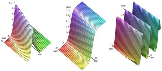
Figure 1. The exact solutions of the generalized SIdV Equation (5) over the time interval $[0,10]$. The left is a bell-shaped solitary wave solution (18) when ${\gamma }_1=1,\delta =2,{\mu }_2=1,{\mu }_3=-1$, and $\epsilon =1$, the middel is an anti-kink-shaped solitary wave solution (39) when $\delta =\frac{1}{2},{\mu }_2=\frac{1}{4},{\mu }_3=1,{\mu }_4=1$, and $\epsilon =-1$, and the right is a periodic solitary wave solution (43) when $\delta =2,{\mu }_2=\frac{-1}{5},{\mu }_3=1,{\mu }_4=-1$, and $\epsilon =1$.

Figure 2. The exact solutions of the generalized SIdV Equation (5) at $t=0$. The left is a singular wave solution (18) when ${\gamma }_1=1,\delta =2,{\mu }_2=1,{\mu }_3=1$, and $\epsilon =1$, the middel is a periodic singular wave solution (19) when $\delta =2,{\mu }_2=-1,{\mu }_3=1,{\gamma }_1=1$, and $\epsilon =1$, and the right is a kink-shaped solitary wave solution (48) when $\delta =1,{\mu }_3=1,{\gamma }_0=1,{\gamma }_1=1,$ and $\epsilon =-1$.

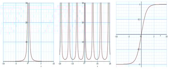
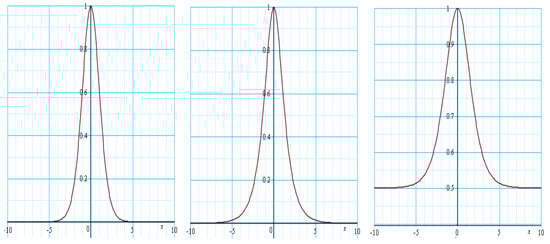
Figure 3. The exact solutions of the generalized SIdV Equation (5) at $t=0$. The left is a bell-shaped solitary wave solution (51); namely, $u(x,t)={sech}^4(\frac{1}{2}x-\frac{4}{3}t)$ when $\delta =1,\gamma =\frac{4}{3},{\gamma }_2=1,{\mu }_2=1$, and ${\mu }_3=1$, the middle is a bell-shaped solitary wave solution (59); namely, $u(x,t)=sech(x-\frac{4}{3}t)$ when $\delta =1,\gamma =\frac{2}{3},{\gamma }_1=1,{\mu }_2=1,{\mu }_4=-1$, and $\epsilon =1$, and the right is a bell-shaped solitary wave solution (60); namely, $u(x,t)=\frac{1}{2}+\frac{1}{2}{sech}^2(\frac{1}{2}x-2t)$ when $\delta =-1,{\gamma }_0=\frac{1}{2},{\gamma }_1=-1,{\mu }_2=1$, and ${\mu }_3=2$.

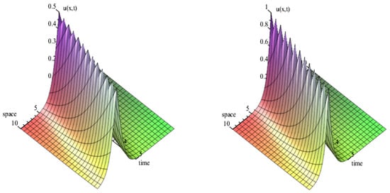
Figure 4. The exact peakon wave solutions of the generalized SIdV Equation (5) over the time interval $[0,5]$. The left side shows a peakon wave solution (44)—namely, $u(x,t)=\frac{1}{2}\left[1-tanh\left(\frac{1}{2}\right|x-t\left|\right)\right]$ when $\delta =\frac{1}{2}$ and ${\mu }_2=1$; and the right side shows a peakon wave solution (55), namely, $u(x,t)=exp(-|x-t\left|\right)$ when $\delta =1,\gamma =1,{\mu }_2=1,$ and ${\gamma }_1=\frac{1}{4}$. The peakon solution is obtained when kink and anti-kink solutions (or two exponential solutions of the opposite forms) move in the same direction with the same speed.

Figure 1 shows a rich array of bounded solutions from a solitary pulse ($\delta =2$) to a kink ($\delta =\frac{1}{2}$) and to a periodic wave ($\delta =2$) for values of $\delta$ other than either 1 or negative 1.

In Figure 2, one can see a singular solitary wave and a singular periodic wave for the $\delta$-value of 2. If the singular solitary pulse is compared to the bounded solitary wave in Figure 1 for $\delta =2$, the only difference is in the choice of ${\mu }_3$. The singular pulse is obtained with a positive ${\mu }_3$, whereas the bounded solitary pulse is found with a negative ${\mu }_3$. Similarly, if one compares parameter values for the singular solitary pulse with the bounded solitary wave in Equation 23) when $\epsilon =1$, it can be observed that the singular pulse is obtained with a positive ${\mu }_3$, whereas the bounded solitary pulse is found with a negative ${\mu }_3$.

Figure 3 presents other bounded solitary pulse solutions (as opposed to the KdV soliton of the ${sech}^2$ form) of the forms of $sech, {sech}^2,$ and ${sech}^4$ for $\delta$ values of either 1 or negative 1.

Figure 4 shows the peaked solutions (peakons) that we are able to find for two different $\delta$ values. Note that a peakon has a discontinuous first derivative at its peak.

4. Conclusions

In this paper, we considered a generalized SIdV equation that is KdV-like, with an advecting velocity given by $\left(3(1-\delta )u+(\delta +1)\frac{u_{xx}}{u}\right)$. Making use of the auxiliary equation method, for different values of $\delta$, we were able to find closed-form expressions for a variety of solutions, both bounded and singular. Interestingly, we showed that the SIdV equation (i.e., when $\delta =1$) has solitary wave solutions of bell type of the forms of sech and ${sech}^4$ in addition to the ${sech}^2$ solution that it shares with the KdV equation (see Figure 3). Further, we even obtained peakon solutions for the SIdV equation ($\delta =1$) and for the generalized SIdV equation when $\delta$ is any value (see Figure 4 when $\delta =\frac{1}{2}$). The solutions found in this work are new and have not been reported elsewhere in the literature. Looking ahead, one could explore to determine whether the generalized SIdV equation possesses multiple kink or bell-type solutions, as was shown for the negative order KdV equation [10]. In addition, one could build on the work in [12] and expand our knowledge to understand how one may be able to employ the SIdV equation in engineering applications such as control theory and image restoration. Our work also demonstrated the versatility of the auxiliary equation in extracting an array of interesting solutions from a KdV-like advection equation.

References

- Ablowitz, M.J.; Clarkson, P.A. Solitons, Nonlinear Evolution Equations and Inverse Scattering; Cambridge University Press: Cambridge, UK, 1991; p. 149. [Google Scholar]
- Hirota, R. Exact solution of the Korteweg-de Vries equation for multiple collisions of solitons. Phys. Rev. Lett. 1971, 27, 1192–1194. [Google Scholar] [CrossRef]
- Crighton, D.G. Applications of KdV. Acta Appl. Math. 1995, 39, 39–67. [Google Scholar] [CrossRef]
- Hershkowitz, N.; Romesser, T. Observations of ion-acoustic cylindrical solitons. Phys. Rev. Lett. 1974, 32, 581. [Google Scholar] [CrossRef]
- Berest, Y.Y.; Loutsenko, I.M. Huygens’ principle in Minkowski spaces and soliton solutions of the Korteweg-de Vries equation. Commun. Math. Phys. 1997, 190, 113–132. [Google Scholar] [CrossRef] [Green Version]
- Gardner, C.S.; Greene, J.M.; Kruskal, M.D.; Miura, R.M. Method for solving the Korteweg-deVries equation. Phys. Rev. Lett. 1976, 19, 1095. [Google Scholar] [CrossRef]
- Sen, A.; Ahalpara, D.P.; Thyagaraja, A.; Krishnaswami, G.S. A KdV like advection-dispersion equation with some remarkable properties. Commun. Nonlinear Sci. Numer. Simul. 2012, 17, 4115–4124. [Google Scholar] [CrossRef] [Green Version]
- Silva, P.L.D.; Freire, I.L.; Sampaio, J.C.S. A family of wave equations with some remarkable properties. Proc. R. Soc. A 2018, 474, 20170763. [Google Scholar] [CrossRef]
- Zhang, G.; He, J.; Wang, L.; Mihalache, D. Kink-type solutions of the SIdV equation and their properties. R. Soc. Open Sci. 2019, 6, 191040. [Google Scholar] [CrossRef] [Green Version]
- Qiao, Z.; Fan, E. Negative-order Korteweg-de Vries equations. Phys. Rev. E 2012, 86, 016601. [Google Scholar] [CrossRef] [Green Version]
- Tsutsumi, M.; Mukasa, T.; Iino, R. On the generalized Korteweg–De Vries equation. Proc. Jpn. Acad. 1970, 46, 921–925. [Google Scholar]
- Xu, D.D.; Zhang, D.J.; Zhao, S.L. The Sylvester equation and integrable equations: I. The Korteweg-de Vries system and sine-Gordon equation. J. Nonlinear Math. Phys. 2014, 21, 382–406. [Google Scholar] [CrossRef] [Green Version]
- Bhatia, R.; Rosenthal, P. How and why to solve the operator equation AX − XB = Y. Bull. Lond. Math. Soc. 1997, 29, 1–21. [Google Scholar] [CrossRef]
- Fan, X.; Yin, J. Two types of traveling wave solutions of a KdV-like advection-dispersion equation. Math. Aeterna 2012, 2, 273–282. [Google Scholar]
- Feng, Q.; Zheng, B. Traveling wave solutions for the fifth-order Sawada-Kotera equation and the general Gardner equation by ()-expansion method. WSEAS Trans. Math. 2010, 9, 171–180. [Google Scholar]
- Zayed, E.; Abdelaziz, M. Exact traveling wave solutions of nonlinear variable coefficients evolution equations with forced terms using the generalized ()-expansion method. Wseas Trans. Math. 2011, 10, 115–124. [Google Scholar] [CrossRef]
- Alzaleq, L.; Manoranjan, V. Exact traveling waves for the Fisher’s equation with nonlinear diffusion. Eur. Phys. J. Plus. 2020, 135, 1–11. [Google Scholar] [CrossRef]
- Yang, X.-F.; Deng, Z.-C.; We, Y.i. A Riccati–Bernoulli sub-ODE method for nonlinear partial differential equations and its application. Adv. Differ. Equ. 2015, 2015, 1–17. [Google Scholar] [CrossRef] [Green Version]
- Wang, M. Exact solutions for a compound KdV-Burgers equation. Phys. Lett. A 1996, 213, 279–287. [Google Scholar] [CrossRef]
- Alzaleq, L.; Manoranjan, V. Analysis of the Fisher-KPP equation with a time-dependent Allee effect. IOP SciNotes 2020, 1, 025003. [Google Scholar] [CrossRef]
- Zhu, S.D. The generalizing Riccati equation mapping method in non-linear evolution equation: Application to (2+1)-dimensional Boiti-Leon-Pempinelle equation. Chaos Solitons Fractals 2008, 37, 1335–1342. [Google Scholar] [CrossRef]
- Biswas, A. Solitary wave solution for the generalized Kawahara equation. Appl. Math. Lett. 2009, 22, 208–210. [Google Scholar] [CrossRef] [Green Version]
- Kudryashov, N.A. Method for finding highly dispersive optical solitons of nonlinear differential equations. Optik 2020, 206, 163550. [Google Scholar] [CrossRef]
- Kudryashov, N.A. One method for finding exact solutions of nonlinear differential equations. Commun. Nonlinear Sci. Numer. Simul. 2012, 17, 2248–2253. [Google Scholar] [CrossRef] [Green Version]
- Parkes, E.J.; Duffy, B.R.; Abbott, P.C. The Jacobi elliptic-function method for finding periodic-wave solutions to nonlinear evolution equations. Phys. Lett. A 2002, 295, 280–286. [Google Scholar] [CrossRef]
- Yu, J.; Sun, Y. Modified method of simplest equation and its applications to the Bogoyavlenskii equation. Comput. Math. Appl. 2016, 72, 1943–1955. [Google Scholar] [CrossRef]
- Yu, J.; Wang, D.S.; Sun, Y.; Wu, S. Modified method of simplest equation for obtaining exact solutions of the Zakharov–Kuznetsov equation, the modified Zakharov–Kuznetsov equation, and their generalized forms. Nonlinear Dyn. 2016, 85, 2449–2465. [Google Scholar] [CrossRef]
- Sun, Y.L.; Ma, W.X.; Yu, J.P.; Khalique, C.M. Exact solutions of the Rosenau–Hyman equation, coupled KdV system and Burgers–Huxley equation using modified transformed rational function method. Mod. Phys. Lett. B 2018, 32, 1850282. [Google Scholar] [CrossRef]
- Veeresha, P.; Prakasha, D.G.; Singh, J. Solution for fractional forced KdV equation using fractional natural decomposition method. Aims Math. 2020, 5, 798–810. [Google Scholar] [CrossRef]
- Baishya, C.; Achar, S.J.; Veeresha, P.; Prakasha, D.G. Dynamics of a fractional epidemiological model with disease infection in both the populations. Chaos Interdiscip. J. Nonlinear Sci. 2021, 31, 043130. [Google Scholar] [CrossRef]
- Baishya, C.; Veeresha, P. Laguerre polynomial-based operational matrix of integration for solving fractional differential equations with non-singular kernel. Proc. R. Soc. A 2021, 477, 20210438. [Google Scholar] [CrossRef]
- Veeresha, P.; Prakasha, D.G.; Kumar, D.; Baleanu, D.; Singh, J. An efficient computational technique for fractional model of generalized Hirota-Satsuma-coupled Korteweg-de Vries and coupled modified Korteweg-de Vries equations. J. Comput. Nonlinear Dyn. 2020, 15, 071003. [Google Scholar] [CrossRef]
- Veeresha, P.; Prakasha, D.G.; Magesh, N.; Christopher, A.J.; Sarwe, D.U. Solution for fractional potential KdV and Benjamin equations using the novel technique. J. Ocean Eng. Sci. 2021, 31, 943–950. [Google Scholar] [CrossRef]
- Sirendaoreji, N.A.; PrakJiongasha, S. Auxiliary equation method for solving nonlinear partial differential equations. Phys. Lett. A 2003, 309, 387–396. [Google Scholar] [CrossRef]
- Alzaleq, L. A Klein-Gordon Equation Revisited: New Solutions and a Computational Method; Washington State University: Pullman, WA, USA, 2016. [Google Scholar]
- Sirendaoreji, N.A. Auxiliary equation method and new solutions of Klein-Gordon equations. Chaos Solitons Fractals 2007, 31, 943–950. [Google Scholar] [CrossRef]
Publisher’s Note: MDPI stays neutral with regard to jurisdictional claims in published maps and institutional affiliations. |
© 2022 by the authors. Licensee MDPI, Basel, Switzerland. This article is an open access article distributed under the terms and conditions of the Creative Commons Attribution (CC BY) license (https://creativecommons.org/licenses/by/4.0/).