Abstract
There is an increasing demand for power production day by day all over the globe; thus, hybrid frameworks have an essential role in producing sufficient power for the desirable load due to increasing power demand. The proposed hybrid renewable energy (HRE) systems are used to provide power in different areas to conquer the intermittence of wind and solar resources. The HRE system incorporates more than one renewable energy (RE) system. In this research article, the optimum power generation of different combinations of RE using different Maximum Power Point Tracking (MPPT) control methods is presented. The Fuel Cell (FC), FC–Photovoltaic (PV), FC–Wind (W), and FC–PV–W systems are developed to examine different MPPT controllers. The results show that the FC–PV–W HRE system produces the maximum power as compared to the FC, FC–PV, and FC–W systems. The FC–PV–W HRE system produces increased power compared to 94.24% from the FC system, 37.17% from the FC–PV hybrid system, and 15.8% from the FC–W hybrid framework with a Perturb and Observe (P&O) controller and, similarly, 74.57% from the FC system, 10.3% from the FC-PV hybrid system, and 31.64% from the FC-W hybrid system using a fuzzy logic (FL) controller, indicating that the best combination is the FC-PV-W hybrid system using an FL controller, which is useful for maximum power generation with reduced oscillations.
1. Introduction
The global demand for electrical energy is gradually increasing, and the search for replacements for fossil fuels is done on a priority basis. Conventional energy sources, such as fossil fuels (FF), are not sustainable and produce greenhouse gas emissions, polluting the environment. The usage of RE frameworks, for example, PV and wind turbine (WT) power, are needed due to a lack of FF supplies and an adverse environment. The use of more than one RE source to create an HRE system has fantastic potential for distributed power generation. PV and WT are primary RE sources, with an FC system as a backup power supply. PV and WT systems are not only environmentally friendly and long-lasting, but they are also well-designed, widely used, and cost-effective. Apart from these RE sources, FC has also been exploited to meet rising energy demand []. Solar PV and WT power generation systems require storage energy units including super capacitors and power backup []. The energy of PV and WT systems is generated and stored in the battery through bright and windy days, and power is released from the battery at night or on cloudy days. Electric energy (EE) is saved for off-peak hours and then used for peak time to smooth power demand []. The negative aspect of WT and PV systems are the irregular natures that make them unreliable. The hybrid system yields a superior prospect for dispersed power generation. A few studies in the literature of power management advocate for an AC link, an ultra-capacitor bank, and power oscillations in hybrid PV, wind, and FC systems [].
The MPPT system allows for increased power transmission from the solar array to the load that must be met, extending the solar PV system’s lifetime []. A few MPPT control approaches have been reported, with the highest power obtained []. PV and WT with FL controller-based MPPT are utilized to maximize the power output by buck and boost power converters, and their duty cycles can be changed []. P&O-based MPPT and Hill Climbing (HC)-based MPPT approaches are the most widely used MPPT methods based on diverse topologies and with diverse efficiency, cost, and complexity []. Aside from these techniques, others have been described to improve the performance of various MPPT systems such as Incremental Conductance (INC) [], Artificial Neural Network (NN), and FL-based MPPT controller [].
P&O methodology is often used to determine the MPP of solar and WT production modules. Without addressing the ecological circumstances, an effortless and cost-effective MPPT algorithm for solar and wind systems was suggested in []. Maoum et al. conducted practical and theoretical studies to assess fast and reliable MPPT strategies for PV systems, such as voltage and current-based MPPT algorithms []. Intelligent MPPT techniques are used to deal by the non-linear properties of solar PV panels []. An FL-based MPPT controller, according to Kamal et al., can offer a static pitch MP coefficient and handle abrupt load fluctuations [].
A scholar built a one-dimensional non-isothermal PEMFC prototype and tested the effects on cell efficiency, thermal responsiveness, and water control over varied outlines and working states to realize the underlying process []. A radial-based function occurs only once in a while. Metamodels indicating the steady-state relationships between stack powers, oxygen, compressor voltage, and stack current were created using NN []. ANFIS and Artificial NN techniques are used to forecast Solid Oxide Fuel Cell (SOFC) efficiency by giving power in addition to heat to a home. The effect proves that the computing time reduction is significant devoid of jeopardizing the validity of the SOFC framework []. WT has been built utilizing the MPPT algorithm, which combines high productivity with a buck DC–DC converter and a microcontroller to do MPPT work consecutively []. The experimental results of the recommended system, which shows the output capacity of near-optimal WG, is increased by 11% to 50% when compared to a WG linked directly to a battery bank rectifier. By altering the emphasis curve for Voc, MP, and Isc, Villalva et al. discovered the non-linear mathematical statement I–V parameters []. Rosli et al. [] presented a multi input power converter (MIPC) in favor of a grid-connected (WT, PV, FC) and battery storage (BS) hybrid framework. The MATLAB/simulation model made it possible to simplify the framework and cut costs. To improve the solar–wind hybrid system, the constant voltage (CV) MPPT approach is applied []. To regulate the desired power grid frequency, Ganji et al. [] anticipated an enhanced fuzzy particle swarm optimization methodology. MP is also extracted from hybrid WT, FC, and ultra-capacitor systems by a second-order sliding mode approach. Khan et al. [] established an FL-based MPPT approach for hybrid PV, WT, and FC systems with varying loads. An ANFIS-based MPPT methodology was presented to integrate the PV, WT, and DG into a hybrid framework. In terms of their ability to produce power and consume it, the modeling results are promising []. The results of a proportional investigation of multiple MPPT strategies used for the wind–PV hybrid framework demonstrate the utility of the ANFIS methodology in stipulations of level of voltage and MPP oscillation mitigation []. It has developed a unique system based on front-end rectifier stage arrangement used for WT/PV hybrid architecture []. In a hybrid solar PV–WT arrangement, the PWM technique of space vector is revealed to change DC output addicted to a voltage in the form of sinusoidal using a single three-phase inverter. For the WT/ PV hybrid, a framework with a general MPPT technique is proposed for energy storage provisions [,], which require comprehensive power handling. Khan et al. [] presented a hybrid framework that combines PV, WT, and FC systems with an MPPT controller and DC–DC converters to give MP at the DC link.
To adhere to the general framework, the complete control is modeled in MATLAB/SIMULINK, and a single dSPACE will complete the controller’s hardware execution. A simulation-based real-time assessment of FL, NN, and ANFIS strategies with solar PV systems built in the MATLAB/dSPACE platform reveals that the ANFIS-based MPPT methodology outperforms the others []. In an energetic prototype of the HRE System [], a WT-based driven self-excited induction generator (SEIG), solar PV, and DC–DC power circuit were created.
RE sources such as solar PV array and WT systems have non-linear output characteristics that vary with radiation, ambient temperature, and wind speed. The systems create extreme output power under specific environmental circumstances. In the methodology, the MPP yield point is a one-of-a-kind yield point that varies according to the environment. MPPT are used in order to attain the MP from PV, WT, FC, and HRE systems. In this paper, different MPPT techniques are used that produced the optimum power. The FL-based MPPT technique provides a better performance of proposed hybrid systems compared to conventional P&O techniques. Figure 1 shows the proposed approach.
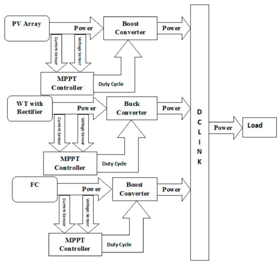
Figure 1.
Proposed approach.
The following steps are used in the methodology in this manuscript:
- Step 1.
- Sense the voltage and current values by the voltage and current sensors from RE sources such as PV, WT, and FC.
- Step 2.
- Use the sensed voltage and current values to design the MPPT controller.
- Step 3.
- These MPPT controllers are used to generate the best possible duty cycle to DC–DC power converters.
- Step 4.
- Respective DC–DC converters are connect with PV, WT, and FC models that produce maximum voltage to the DC link as per given input patterns.
- Step 5.
- The DC link is set to control the voltage of all renewable energy sources, which are connected in parallel with the DC link.
- Step 6.
- Finally, add all currents and make constant all voltage in the DC link due to the parallel connection of renewable energy sources.
- Step 7.
- Using all renewable energy sources with MPPT controllers generates the maximum power to the load.
The following is a breakdown of the paper’s structure: Section 2 depicts the many renewable energy source combinations that have been proposed. Section 3 describes the various types of MPPT controllers. The simulation model of several entire systems is discussed in Section 4. Section 5 contains the findings and discussions. Finally, Section 6 outlines the conclusions.
2. Proposed Combinations of Renewable Energy Sources
In this research, many combinations have been made with different MPPT techniques, and rather than finding which combination is best for all systems, the existing research explored different MPPT techniques for an individual renewable energy system or a hybrid renewable energy system. In this context, the following points are defined as novel work in this manuscript.
- Modeling of different controllers for different combinations of RE sources.
- Calculate the optimum duty cycle in favor of the DC–DC power converters for achieving the MP.
- Investigations of the best combinations with MPPT controllers.
The proposed system comprises an FC system (1 kW), WT system (1.2 kW), and the PV system (0.8 kW). All the above considered RE systems are joined in parallel with individual power (DC–DC) converters and various MPPT controllers at a DC link. The comprehensive systems and combinations are simulated for various operating conditions of the RE sources. For analysis, the first system is the only FC framework, as illustrated in Figure 2. The second combination is an FC–PV hybrid framework, as illustrated in Figure 3. The third combination is an FC–W hybrid framework, as illustrated in Figure 4. The fourth combination is an FC–PV–W hybrid system, as illustrated in Figure 5. Where, I and V represents the measured value of current and voltage respectively, and W represents the wind system.
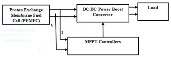
Figure 2.
Proposed PEM–FC framework with different MPPT controllers.
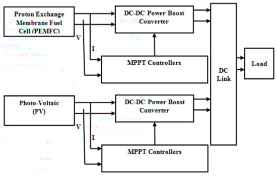
Figure 3.
Proposed combination of FC–PV systems with different MPPT controllers.
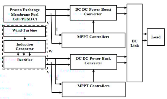
Figure 4.
Proposed combination of FC–W systems with different MPPT controllers.
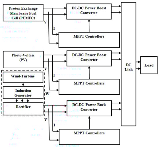
Figure 5.
Proposed combination of FC–PV–W systems with different MPPT controllers.
3. Proposed Different Types of MPPT Controllers
RE systems have non-linear output characteristics that vary with radiation, ambient temperature, wind speed, and hydrogen fuel. The systems create extreme output power under specific environmental circumstances. The MPP yield point is a one-of-a-kind yield point that varies according to the environment. MPPT are used in order to attain the MP from PV, WT, FC, and HRE systems. The efficiency of the MPPT method can increase with alteration the sampling time (Ts) according to the energetic converter, as shown in this work. The sample interval should be set as small as possible, devoid of generating unsteadiness during the availability of sun and wind, when the MPP of the non-linear renewable energy system moves very slowly. Using the MPPT technique produces samples of voltage and current of RE sources rapidly as well, it may be vulnerable to errors produced by the PV array and converter system’s transient behavior, causing the MPP to be temporarily missed. As a result, the technique may get baffled, the energy efficiency may deteriorate, and the operating point may become unsteady, leading to disordered behaviors. The method given in this research is to choose Ts based on the dynamics of the converter.
- A.
- MPPT Controller based on P&O
The P&O-based MPPT algorithm is generally employed due to its easy structure and low quantity of observed constraints []. It operates by periodically perturbing (moving up or moving down) a model’s terminal voltage and matching the RE framework output power in order to alter a sequence. The perturbation will stay in the alike path in the next cycle if power is growing; else, the perturbation will reverse direction. Figure 6 shows a representation of the flowchart. Pushing the operating point to function near the MPP includes two disadvantages in some situations: fluctuations in the region of MPP emerge in a steady-state condition. This technique has disadvantage that cause the available energy to be dissipated. Under rapidly changing environmental conditions, this technique may cause the operational point (OP) to be moved far from the MPP instead of near it [,].
- A.1
- Mathematical Modeling of P&O MPPT controller
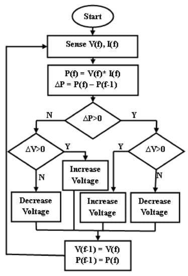
Figure 6.
Flowchart of P&O method.
V(f) and I(f) are sensed by sensors from PV, WT, and FC models. Now, PV is consider for the derivation of P&O techniques.
After delay, the voltage is V(f − ∆f) and current is
I(f − ∆f).
The current power is
P(f) = V(f) × I(f).
After delay, the power is
P(f − ∆f) = V(f − ∆f) × I(f − ∆f).
Now, find the differences in the power between the current power and after delay power, i.e.,
∆P = P(f) − P(f − ∆f)
and similarly,
∆V = V(f) − V(f − ∆f).
To check the conditions
Condition 1, ∆P = 0 that means the OP is about the MPP.
Condition 2, ∆P > 0, subsequently check the following conditions:
Condition 1′, ∆V > 0 then, it signifies that the operational point is on the MPP’s left side.
Condition 2′, ∆V < 0 then, it signifies that the OP is on the MPP’s right side.
This method is done indefinitely until the MPP is attained. As a result, the P&O algorithm always represents a compromise between increments and sampling rate.
- B.
- MPPT Controller Based on FLC
In comparison to the P&O MPPT control technique, the FL MPPT algorithm is presented to achieve maximum power and reduce fluctuations [,]. Figure 7 depicts the fundamental architecture of a fuzzy logic controller. It also affords normalization parameters. The FL controller in this technique comprises crisp inputs, fuzzification, rule-based inference, defuzzification, and crisp output, as shown in Figure 7. The FL designer is shown in Figure 8 and was created using the MATLAB/SIMULINK platform. As indicated in Figure 9 and Figure 10, the two inputs (current-I and voltage-V) will fuzzify by normalized fuzzy sets and three triangular membership functions. As seen in Figure 11, the output variable (duty-cycle) is a triangular MF followed by a normalized fuzzy set of Small (S), Medium (M), and High (H).
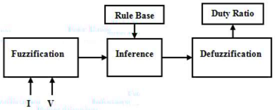
Figure 7.
Fuzzy logic approach.
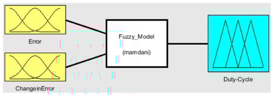
Figure 8.
FL designer.
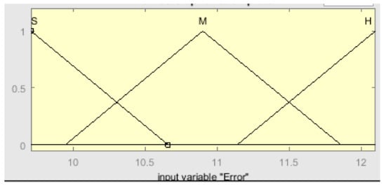
Figure 9.
Membership function of input variable in terms of error.
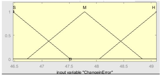
Figure 10.
Membership function of input variable in terms of change in error.
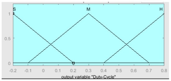
Figure 11.
Membership function of output variable in terms in duty cycle.
The produced fuzzy sets must be compared to the rule-base after the crisp inputs have been fuzzified. The rule-base is a collection of “If premise Then consequence” rules organized based on the design system’s information and occurrence. The inference minimum operator calculates the premise. The first part of the rule is this: The operator compares the rules, selects the least restrictive choice, and is ON in each input membership function. The defuzzification stage in the FL controller construction gets the inferred fuzzy set and converts it back to a crisp output or else an actual continuous number. The FL controller has defined rules in the rule editor, as illustrated in Table 1. Figure 12 shows the surface viewer of an FL-based MPPT controller. Error, E(f) and change in Error, ∆E(f) are inputs of FLC, as shown in Figure 8. The user has complete control over the linguistic variables. It utilizes the approximation because dP(f)/dV(f) (or ∆P(f)/∆V(f) vanish at the MPP. The equations shown below are extremely useful and regularly utilized. The linguistic variables are created from the calculated values of E and ∆E.
E(f) = (P(f) − P(f − 1))/(V(f) − V(f − 1))
∆E(f) = E(f) − E(f − 1)

Table 1.
Fuzzy rule base.
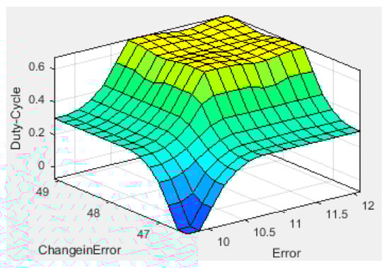
Figure 12.
Surface Viewer of FLC.
Mathematical implementation for a fuzzy-logic based system is available in several publications. In this regard, the reader may follow the references [,,,,,,,].
As mentioned in the introduction, different strategies have been used to solve the partial shading difficulty of solar PV systems. The majority of these approaches are complicated and computationally intensive, and they have a negative influence on grid stability due to power interruption during PV scanning. To address the issue of partial shading, an MPPT algorithm based on FLC is developed, which can enhance output power when partial shading occurs. Since the proposed MPPT technique was created to adapt the FLC, the original fuzzy MPPT is discussed in detail in Section 3. The flow chart calculation using the FL controller for the photovoltaic/wind/FC is shown in Figure 13.
- B.1
- Basic Impression of Fuzzy Differential Equations
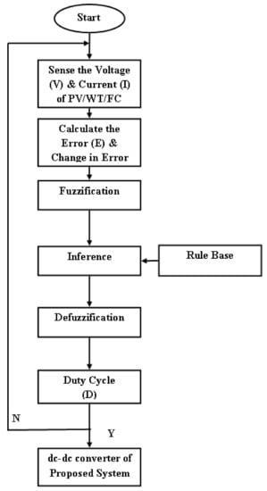
Figure 13.
Flowchart calculation using the FL controller for PV/W/FC.
Let Y be a set that is not empty. The membership function u: Y [0, 1] characterizes a fuzzy set u in Y. Therefore, the degree of association of a component y in the fuzzy set m for all y, Y can be understood as m(y).
Definition 1.
Assume Fn is the space containing of the entire compressed and turned in fuzzy sets lying on Rn. Assume m, u ∈ Fn. If here, n ∈ Fn such that m = u ⊕ n, after that, n is referred to as the H-difference between m and u and is indicated by m ⊖ u.
Definition 2.
Assume F: S → Fn and t0 ∈ S. The function F is differentiated at f0 if
- (a)
- A component F′(f0) ∈ Fn is present for all g > 0 satisfactorily near 0; here, F(f0 − g) ⊖ F(f0), F(f0) ⊖ F(f0 − g) and the limits are equal to F′(f0).
- (b)
- An element F′(f0) ∈ Fn is present for all g < 0 satisfactorily near 0; there are F(f0 + g) ⊖ F(f0), F(f0) ⊖ F(f0 − g), and the limits are equal to F′(f0).
It is important to remember that if F is the differentiable in the first form (a), it is not differentiable in the second form (b) and vice versa.
Know that F: S → F is a function and [F(f)]α = [gα(f), hα(f)] for each α ∈ [0, 1]. The fundamental finding in favor of calculating a fuzzy differential equation (FDE) is as follows.
Definition 3.
Assume F: S → F represents the function.
- (i)
- If F is differentiated in the first form (a), after that, gα and fα are called differentiable functions.
[F′(f)]α = [f′α(f), g′α(f)].
- (ii)
- If F is differentiable in the second form (b), then fα and gα are also differentiable functions and
[F′(f)]α = [g′α(f), f′α(f)].
Definition 4.
Assume F: S → F represents the incessant function. Then
- (i)
- If F subsists differentiate in the first form (a), after that, F′ is an integrable if and only if F (a) ≺ F (f) for all f ∈ S.
- (ii)
- If F represents the differentiable in the second form (b), then F′ is an integrable if and only if F (f) ≺ F (a) for all f ∈ S.
- B.2
- Fuzzy Differential Equations
Regard the DFE as
y0 is the fuzzy interval, and F: [c, d] × F → F represents the incessant fuzzy mapping. The selection of the derivative: during the second form or during the first form determines the solution of the FDE (13). Definition-2’s Equations (available in point (a) and (b) of Definition-2 as Equations (8) and (9) respectively) provide a method for solving the FDE (13). For this, assume [y (f)]α = [mα (f), uα (f)] and
[F (f, y(f))]α = [gα(f, mα(f), uα(f)), hα(f, mα(f), uα(f))].
Case in point 1: Assume the FDE
where the initial condition y0 and λ > 0 are symmetric triangular fuzzy numbers by support [−c, c]; i.e., [y0]α = [−c (1 − α), c (1 − α)] = (1 − α) [−c, c].
The DFE system will be as follows if y′(f) is treated in the first form (a):
m′α(f) = −λuα(f), mα(0) = −c(1 − α)
u′α(f) = −λmα(f), uα(0) = c(1 − α).
The clarification of this structure is mα(f) = −c(1 − α)eλf and uα(f) = c(1 − α)eλf. As a result, level sets exist for the fuzzy function y(f) solving (14).
[y(f)]α = [−c(1 − α)eλf, c(1 − α)eλf] for all f ≥ 0.
The fuzzy differential system will be as follows if y′(f) is treated in the second form (b):
m′α(f) = −λmα(f), mα(0) = −c(1 − α)
u′α(f) = −λuα(f), uα(0) = c(1 − α).
The clarification of this structure is mα(f) = −c(1 − α)e−λf and uα(f) = c(1 − α)e−λf. Hence, level sets exist for the fuzzy function y(f) solving (14).
[y(f)]α = [−c(1 − α)e−λf, c(1 − α)e−λf] for all f ≥ 0.
MATLAB/SIMULINK is a tool that is used for modeling and evaluating energetic systems that are interactive. MATLAB/SIMULINK is deeply linked with state flow for modeling event-driven behavior and interfaces easily with MATLAB. SIMULINK is a programming language that is built on top of MATLAB. Building pieces from the SIMULINK library can be used to create a SIMULINK model for the given problem. Without writing any programs, the solution curves can be retrieved from the model. A MATLAB/SIMULINK-based model can be built for the following expressions of two differential equations.
The SIMULINK parameters can be adjusted according to the problem as soon as the model is built. By running the model, it can get the solution to the system of differential equations in the display block (or scope) [].
4. Simulation Model of Complete Systems
As a simulation model using MATLABTM/SIMULINKTM, Figure 14 illustrates the proposed framework configuration composed of an FC, boost power converter, different MPPT controllers, and resistive load. Similarly, in Figure 15, the proposed HRE system configuration comprises an FC, PV with an individual boost converter and different MPPT controllers, and a resistive load. An FC with a boost converter, WT linked to an induction generator with a universal bridge rectifier, a buck converter, different MPPT controllers, and a resistive load are revealed in Figure 16. The suggested HRE arrangement is publicized in Figure 17, which includes an FC, PV with an individual boost converter, WT linked to an induction generator with a universal bridge rectifier and a buck converter, various MPPT controllers, and a resistive load. The input patterns for the PV, WT, and FC frameworks are illustrated in Figure 18, Figure 19 and Figure 20. The weather is not always the same; it keeps on changing, so we have made the input pattern changing, as shown in the figures above. In this regard, the change of environmental circumstances for example irradiation, temperature, and wind are input variables for the PV and WT systems. This situation is also called the partial shading condition. Therefore, we consider the input pattern as shown in Figure 17, Figure 18 and Figure 19 in this article. Although the changes in wind speed (WS) and solar irradiation (SR) are just stepping changes, they can never happened in the earth because meteorological circumstances are forever varying. These ethics are preferred to fluctuate between the PV panels’ and WT frameworks’ possible operating ranges between minimum and maximum to test the framework’s operation for these fluctuations. Figure 21 and Figure 22 depict the P&O and FL controller subsystem. Table 2, Table 3 and Table 4 show the parameters of FC and PV by individual boost converters and WTIG by a buck converter.
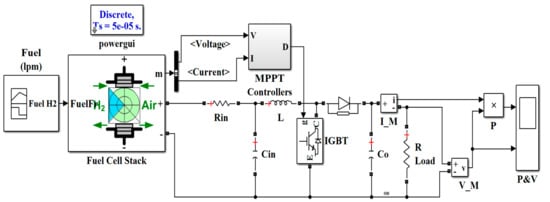
Figure 14.
Simulation model of FC system with MPPT controller.
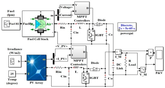
Figure 15.
Simulation model of FC–PV system with MPPT controller.
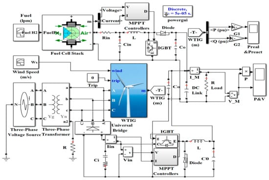
Figure 16.
Simulation model of FC–W system with MPPT controller.
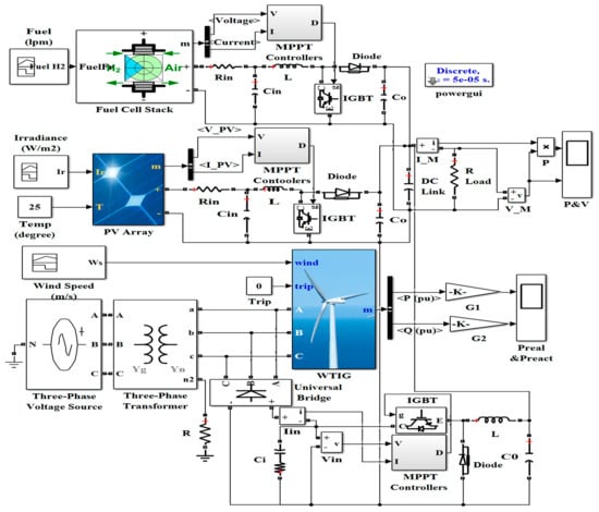
Figure 17.
Simulation model of FC–PV–W framework with MPPT controller.
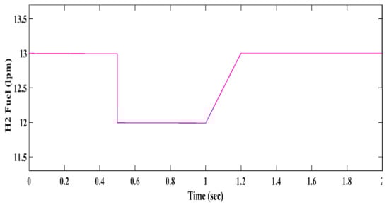
Figure 18.
Hydrogen (fuel) input pattern for FC framework.
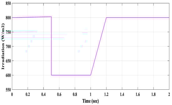
Figure 19.
Irradiation pattern of input for PV system.
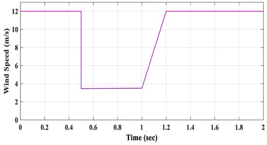
Figure 20.
Wind speed input pattern for wind turbine framework.
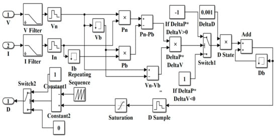
Figure 21.
Subsystem of P&O-based control method.
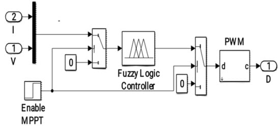
Figure 22.
Subsystem of fuzzy logic controller.
Table 2.
Specifications of FC system.
Table 3.
Specifications of PV system.
Table 4.
Specifications of WT system.
Furthermore, in this scenario, the load is fixed, which would not be the case in practice. The load, on the other hand, is fixed in order to monitor the operation of the RE conversion systems and the FC system for changes in the amount of power delivered by RE sources, which would be feasible to see if the load was not constantly changing. When RE sources such as PV and WT are not working effectively, the FC acts as a storage system (battery backup) that produces power to the load or controls the desired power to the DC link. It fluctuates depending on the difference in the power shortfall from RE sources at different times. Transportation, industrial/commercial/residential constructions, and long-term grid energy storage in reversible systems are all possible applications for FCs. An FC is a device that produces electrical energy by using the chemical energy of hydrogen (H2). When hydrogen is used as a fuel, only electricity, water, and heat are created. In this regard, the FC is unique in that they may function well on a variety of fuels and feedstock.
The load is fixed every second, and the hybrid system’s performance is evaluated for a fluctuation at the MPP. Figure 17 depicts the power at several different locations. The load is constant, and the amount of power produced from RE sources is insufficient to fulfill it; thus, the FC is employed to meet it. The creation and deployment of a solar PV–wind–FC HRE system are with an energy management system (EMS). Experiments were conducted to see how effective the suggested energy management system was with a variety of RE sources and load demand fluctuations. The DSPACE controller’s EMS and control techniques can be created through rapid control prototyping. The outcomes of the testing disclose that the system is adaptive and competent with handling a wide range of renewable energy sources as well as fixed load requirements. The controller makes it possible to construct an effective energy management system. This test bench will be used to develop future testing in the field of HRES, including a variety of case scenarios and control algorithms. As shown in Figure 21, the efficiency of the P&O technique can improve by altering the sample rate according to the energetic converter. Furthermore, inverter current saturation is critical, as large currents might harm or shorten the inverter’s lifespan.
5. Results and Discussions
In this research article, an HRES has been simulated and estimated. The simulation analysis of proposed systems is performed using MATLABTM/SIMULINKTM and different MPPT controllers. The output characteristics of power and voltage for FC, FC–PV, FC–W and FC–PV–W respectably using a conventional P&O MPPT controller are shown in Figure 23, Figure 24, Figure 25 and Figure 26. Figure 27, Figure 28, Figure 29 and Figure 30 show the output characteristics of power and voltage for FC, FC–PV, FC–W and FC–PV–W respectively using the FL-based technique. Figure 31 and Figure 32 demonstrate the comparative output characteristics of power and voltage for proposed systems and combinations using a conventional P&O MPPT controller. Similarly, Figure 33 and Figure 34 illustrate the comparative output characteristics of power and voltage for all the given proposed systems using an FL-based MPPT controller.
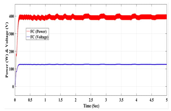
Figure 23.
Power and voltage characteristics of FC system using the P&O-based MPPT method.
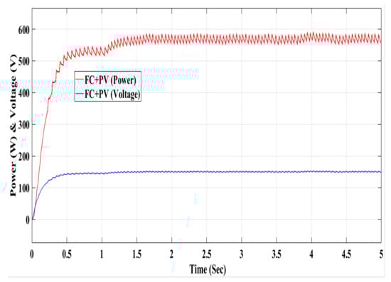
Figure 24.
Power and voltage characteristics of the FC–PV model using the P&O based MPPT method.
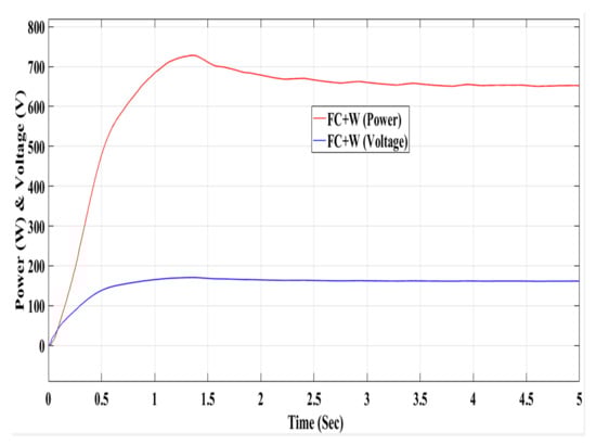
Figure 25.
Power and voltage characteristics of the FC–W Model using the P&O-based MPPT method.
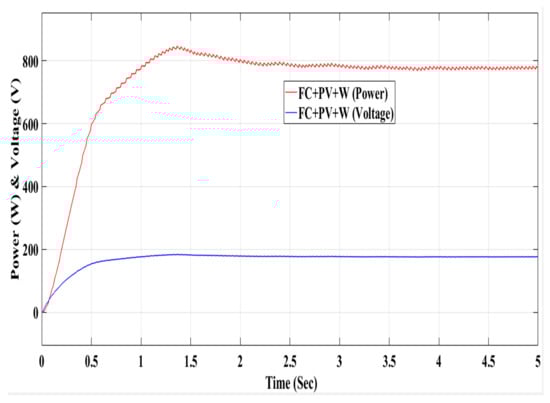
Figure 26.
Power and voltage characteristics of the FC–PV–W model using the P&O-based MPPT method.
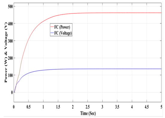
Figure 27.
Power and voltage characteristics of the FC model using a fuzzy logic controller.
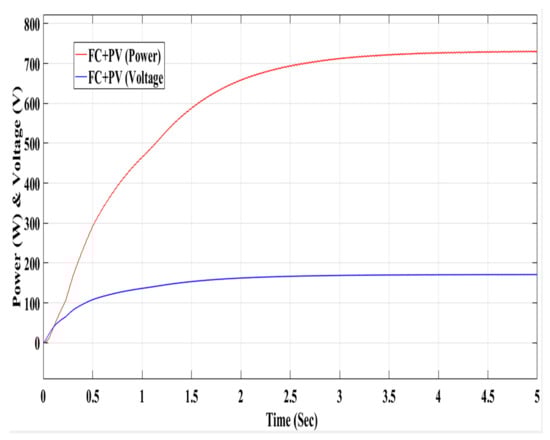
Figure 28.
Power and voltage characteristics of the FC–PV model using a fuzzy logic controller.
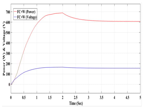
Figure 29.
Power and voltage characteristics of the FC–W model using a fuzzy logic controller.
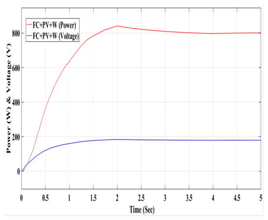
Figure 30.
Power and voltage characteristics of the FC–PV–W model using a fuzzy logic controller.
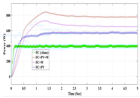
Figure 31.
Comparative characteristics of power in the FC, FC–PV, FC–W, and FC–PV–W models using the P&O controller.
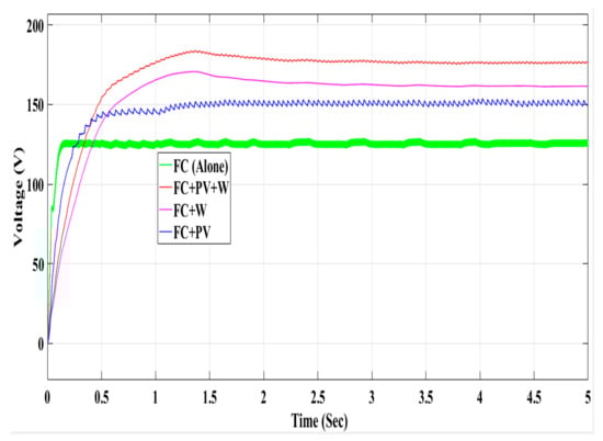
Figure 32.
Comparative characteristics of voltage in the FC, FC–PV, FC–W, and FC–PV–W models using the P&O controller.
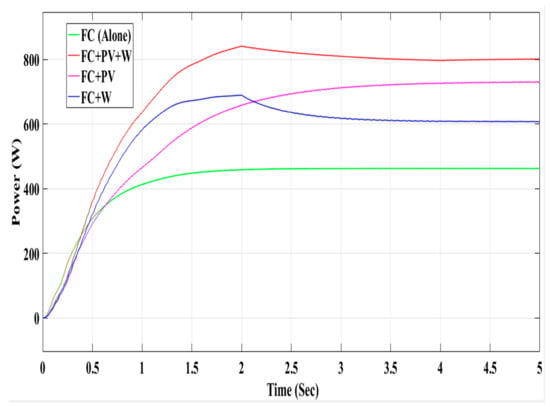
Figure 33.
Comparative characteristics of power in the FC, FC–PV, FC–W and FC–PV–W models using a fuzzy logic controller.
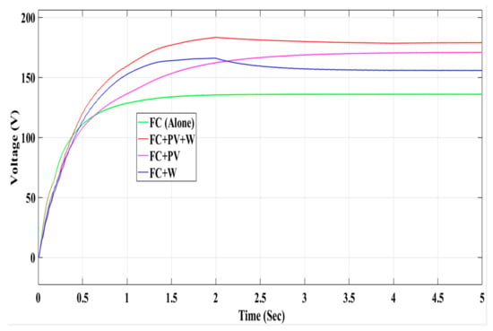
Figure 34.
Comparative characteristics of voltage in the FC, FC–PV, FC–W and FC–PV–W models using a fuzzy logic controller.
As per the analysis of different renewable energy frameworks with various maximum power point tracking controllers, the FC system produces maximum power to the load continuously, but solar and WT systems do not produce continuous power to the load. Therefore, the fuel cell system is the better option to connect with the hybrid system which fulfills the demand of load when sun and wind are not given in the environment. Figure 17 depicts the proposed system. It is separated into three sections:
- (i)
- RE sources backed by an FC, similar to a storage system, and their converters connected to the DC link;
- (ii)
- Load-side converter and single-phase load; and
- (iii)
- Real time-based MPPT controller implementing the EMS. The WECS is made up of a WT with an induction generator. When the electrical power produced by solar PV–WT is a smaller amount than the load requirement, the solar PV array and wind system are controlled with MPPT.
Many combinations with different MPPT techniques have been made in this research, and the goal is to determine which combination is the best with which techniques; rather, existing research has been done with different MPPT techniques for an individual renewable energy system or a hybrid renewable energy system. Generally, renewal energy sources produce non-linear output. MPPT is required for producing maximum power with desirable load from renewable energy sources in variable ecological conditions. Using the proposed systems with MPPT techniques produces the maximum power at continuous mode. It also reduces the fluctuations about the maximum power point. In this article, different combinations with different MPPT techniques are studied and analyzed with various environmental conditions.
In this article, the various combinations of systems such as FC, FC–PV, FC–W, and FC–PV–W are used to find the most feasible combinations for different MPPT controllers such as P&O and FLC. Using the P&O MPPT controller-based proposed configuration, it is clearly seen that the values of the output power are 399 W, 565 W, 652 W, and 775 W, respectively, and the output voltage values are 125 V, 150 V, 161 V, and 175 V, respectively, having a simulation time of 5 s.
Using the FL controller-based proposed system, it is found that the output power values are 460 W, 728 W, 610 W, and 803 W, respectively, and the output voltage values are 135 V, 170 V, 155 V, and 179 V, respectively, having a simulation time of 5 s.
An individual renewable energy system cannot transfer maximum power to the load itself due to impedance mismatch. A MPPT system can be employed with individual system and have the maximum power. The proposed MPPT-based system has been developed using a DC–DC power converter. If one system does not give power, then the other system gives power, so a hybrid system is more beneficial so that the load keeps receiving continuous power. Only individual systems are connected with MPPT and without MPPT techniques. In this manuscript, the MPPT systems produce maximum power and reduce the fluctuations about the MPP. Without the MPPT technique, the systems produce non-linear output; therefore, this power is not usable in the system.
Finally, the FC–PV–W combination outperforms the other considered systems and combinations for both MPPT controllers. Table 5 shows a comparison of power and voltage in various configurations of frameworks using different MPPT controllers.
Table 5.
Power and voltage comparisons in various combinations using different MPPT controllers.
6. Conclusions
Due to impedance mismatch, an individual renewable energy system cannot transfer maximum power to the load. An MPPT system can be used with specific systems to get the most power out of them. Using a buck–boost-type DC–DC converter, a proposed MPPT system has been constructed. If one system fails to provide power, the other will, making the hybrid system more advantageous in terms of ensuring that the load receives continuous power. Only individual systems are connected with MPPT and without MPPT approaches in a hybrid system without MPPT and with MPPT. In this paper, MPPT systems are used to generate maximum power while reducing MPP swings. Since systems without the MPPT approach provide non-linear output, these powers cannot be used in the system. In this paper, the various combinations of systems such as FC, FC–PV, FC–W, and FC–PV–W are used to realize the most possible combinations for various MPPT controllers such as P&O and FLC. It is found that the output power production is 399 W for FC, 565 W for FC–PV, 652 W for FC–W, and 775 W for FC–PV–W systems using a P&O MPPT controller, and 460 W for FC, 728 W for FC–PV, 610 W for FC–W, and 803 W for FC–PV–W systems using an FL–based MPPT controller, which proves that the FC–PV–W system is the most useful. After conducting a comparative investigation of various frameworks using FL MPPT controllers, a combination of various systems provides enhanced control compared to a conservative P&O MPPT controller. Still, the combination of FC-W using P&O offers improved control compared to an FL-based MPPT controller. Therefore, the FC–PV–W with an FL controller is the most feasible combination for MP generation over other combination systems.
RE sold to the grid with various tracking techniques should be the subject of more research. The best DC–DC converter can be set up to help achieve maximum efficiency while maximizing potential power. The proposed work can be implemented in a real-time system and can be analyzed to validate the simulation results of the proposed system with real-time system results.
Author Contributions
Conceptualization, M.J.K., L.M., H.M. and M.A.A.; methodology, M.J.K., L.M., H.M. and M.A.A.; software, M.J.K., L.M., H.M., M.E.N. and M.A.A.; validation, M.J.K., L.M., H.M., M.E.N. and M.A.A.; formal analysis, M.J.K., L.M., H.M. and M.A.A.; investigation, M.J.K., L.M., H.M. and M.A.A.; resources, M.J.K., L.M., H.M., M.E.N. and M.A.A.; data curation, M.J.K., L.M., H.M., M.E.N. and M.A.A.; writing—original draft preparation, M.J.K., L.M., H.M. and M.A.A.; writing—review and editing, M.J.K., L.M., H.M., M.E.N. and M.A.A.; visualization, M.J.K., L.M., H.M., M.E.N. and M.A.A.; supervision, L.M. and M.E.N.; project administration, H.M. and M.A.A.; funding acquisition, H.M. and M.A.A. All authors have read and agreed to the published version of the manuscript.
Funding
The authors extend their appreciation to the Researchers Supporting Project at King Saud University, Riyadh, Saudi Arabia, for funding this research work through the project number RSP-2021/278.
Institutional Review Board Statement
Not applicable.
Informed Consent Statement
Not applicable.
Data Availability Statement
Not applicable.
Acknowledgments
The authors would like to acknowledge the support from King Saud University, Saudi Arabia. The authors would like to acknowledge the support from Intelligent Prognostic Private Limited Delhi, India Researcher’s Supporting Project.
Conflicts of Interest
The authors declare no conflict of interest.
Abbreviations
| ∆E | Change of Error | MF | Membership Function |
| BS | Battery Storage | MIPC | Multi-Input Power Converter |
| Cin | Internal Capacitance | MP | Maximum Power |
| Co | Output Capacitance | MPP | Maximum Power Point |
| CV | Constant Voltage | MPPT | Maximum Power Point Tracking |
| D | Duty Cycle | MPSO | Modified PSO |
| DFIG | Doubly-Fed Induction Generators | NN | Neural Network |
| E | Error | OP | Operating Point |
| EE | Electrical Energy | P&O | Perturb and Observe |
| FC | Fuel Cells | PEM | Proton Exchange Membrane |
| FF | Fossil fuels | PEM-FC | Polymeric Exchange Membrane Fuel Cell |
| FL | Fuzzy Logic | PSO | Particle Swarm Optimization |
| FOCV | Fractional Open-Circuit Voltage | PV | Photo-voltaic |
| Fs | Switching Frequency | RE | Renewable Energy |
| GA | Genetic Algorithm | Rin | Internal Resistance |
| H | High | S | Small |
| HC | Hill Climbing | SPV | Solar Photovoltaic |
| HRE | Hybrid Renewable Energy | UC | Ultra-Capacitor |
| HRES | Hybrid Renewable Energy Sources | V | Voltage |
| IFPSO | Improved Fuzzy Particle Swarm Optimization | W | Wind |
| INC | Incremental Conductance | WT | Wind Turbine |
| L | Inductor | WTG | Wind Turbine Generators |
| M | Medium |
References
- Rubbia, C. Today the world of tomorrow- The energy challenge. Energy Convers. Manag. 2006, 47, 2695–2697. [Google Scholar] [CrossRef]
- Zahran, M. Photovoltaic hybrid systems reliability and availability. J. Power Electron. 2003, 3, 145–150. [Google Scholar]
- Kaldellis, J.K.; Fragos, P.; Kapsali, M. Systematic experimental study of the pollution deposition impact on the energy yield of photovoltaic installations. Renew. Energy 2011, 36, 2717–2724. [Google Scholar] [CrossRef]
- Dursun, E.; Kilic, O. Comparative evaluation of different power management strategies of a stand-alone PV/Wind/PEMFC hybrid power system. Int. J. Electr. Power Energy Syst. 2012, 34, 81–89. [Google Scholar] [CrossRef]
- Khan, M.J.; Mathew, L. Different Kinds of Maximum Power Point Tracking Control Method for Photovoltaic Systems: A Review. Arch. Comput. Methods Eng. 2017, 24, 855–867. [Google Scholar] [CrossRef]
- Esram, T.; Chapman, P.L. Comparison of Photovoltaic Array Maximum Power Point Tracking Techniques. IEEE Trans. Energy Convers. 2007, 22, 439–449. [Google Scholar] [CrossRef] [Green Version]
- Jiang, J.A.; Huang, T.L.; Hsiao, Y.T.; Chen, C.H. Maximum power tracking for photovoltaic power systems. Tamkang J. Sci. Eng. 2005, 8, 147–153. [Google Scholar]
- Ahn, C.W.; Choi, J.Y.; Lee, D.-H.; An, J. Adaptive Maximum Power Point Tracking Algorithm for Photovoltaic Power Systems. IEICE Trans. Commun. 2010, 93, 1334–1337. [Google Scholar] [CrossRef]
- Safari, A.; Mekhilef, S. Simulation and Hardware Implementation of Incremental Conductance MPPT With Direct Control Method Using a Cuk Converter. IEEE Trans. Ind. Electron. 2011, 58, 1154–1161. [Google Scholar] [CrossRef]
- Kumaresan, N.; Kavikumar, J.; Ratnavelu, K. Simulink Approach to Solve Fuzzy Differential Equation under Generalized Differentiability. Int. J. Math. Comput. Sci. 2012, 6, 453–456. [Google Scholar]
- Giraud, F.; Salameh, Z. Steady-state performance of a grid-connected rooftop hybrid wind-photovoltaic power system with battery storage. IEEE Trans. Energy Convers. 2001, 16, 1–7. [Google Scholar] [CrossRef]
- Masoum, M.A.S.; Dehbonei, H.; Fuchs, E.F. Theoretical and experimental analyses of photovoltaic systems with voltage and current-based maximum power-point tracking. IEEE Trans. Energy Convers. 2002, 17, 514–522. [Google Scholar] [CrossRef] [Green Version]
- Alabedin, A.M.Z.; El-Saadany, E.F.; Salama, M.M.A. Maximum power point tracking for Photovoltaic systems using fuzzy logic and artificial neural networks. In Proceedings of the IEEE Conference on Power and Energy Society General Meeting, Detroit, MI, USA, 24–28 July 2011; pp. 1–9. [Google Scholar]
- Kamal, E.; Koutb, M.; Sobaih, A.A.; Abozalam, B. An intelligent maximum power extraction algorithm for hybrid wind–diesel-storage system. Int. J. Electr. Power Energy Syst. 2010, 32, 170–177. [Google Scholar] [CrossRef]
- Rowe, A.; Li, X. Mathematical modeling of proton exchange membrane fuel cells. J. Power Sources 2001, 102, 82–96. [Google Scholar] [CrossRef] [Green Version]
- Hasikos, J.; Sarimveis, H.; Zervas, P.L.; Markatos, N.C. Operational optimization and real-time control of fuel-cell systems. J. Power Sources 2009, 193, 258–268. [Google Scholar] [CrossRef]
- Entchev, E.; Yang, L. Application of adaptive neuro-fuzzy inference system techniques and artificial neural networks to predict solid oxide fuel cell performance in residential microgeneration installation. J. Power Sources 2007, 170, 122–129. [Google Scholar] [CrossRef]
- Koutroulis, E.; Kalaitzakis, K. Design of a maximum power tracking system for wind-energy-conversion applications. IEEE Trans. Ind. Electron. 2006, 53, 486–494. [Google Scholar] [CrossRef]
- Villalva, M.G.; Gazoli, J.R.; Filho, E.R. Comprehensive Approach to Modeling and Simulation of Photovoltaic Arrays. IEEE Trans. Power Electron. 2009, 24, 1198–1208. [Google Scholar] [CrossRef]
- Foti, S.; Testa, A.; De Caro, S.; Tornello, L.; Scelba, G.; Cacciato, M. Multi-Level Multi-Input Converter for Hybrid Renewable Energy Generators. Energies 2021, 14, 1764. [Google Scholar] [CrossRef]
- Jahannoush, M.; Nowdeh, S.A. Optimal designing and management of a stand-alone hybrid energy system using meta-heuristic improved sine–cosine algorithm for Recreational Center, case study for Iran country. Appl. Soft Comput. 2020, 96, 106611. [Google Scholar] [CrossRef]
- Alabedin, A.Z.; El-Saadany, E.F.; Salama, M.M.A. Maximum Power Extraction For Hybrid Solar Wind Renewable Energy System Based on Swarm Optimization. Int. J. Renew. Energy Res. 2021, 11, 1215–1222. [Google Scholar]
- Ganji, E.; Moghaddam, R.K.; Toloui, A.; Taghizadeh, M. A new frequency control approach for isolated WT/FC/UC power system using improved fuzzy PSO & maximum power point tracking of the WT system. J. Intell. Fuzzy Syst. 2014, 27, 1963–1976. [Google Scholar]
- Sharma, M.K.; Soni, S.U. Performance Analysis of a Standalone PV-Wind-Diesel Hybrid System using ANFIS based Controller. Int. J. Comput. Appl. 2016, 147, 18–23. [Google Scholar]
- Ali, N. An ANFIS Based Advanced MPPT Control of a Wind-Solar Hybrid Power Generation System. Int. Rev. Model. Simul. 2014, 7, 638–643. [Google Scholar]
- Kumar, P.S.; Chandrasena, R.P.S.; Ramu, V.; Srinivas, G.N.; Babu, K.V.S.M. Energy Management System for Small Scale Hybrid Wind Solar Battery Based Microgrid. IEEE Access 2020, 8, 8336–8345. [Google Scholar] [CrossRef]
- Doncy, J.K.; Davis, S. Integrated flyback converter with MPPT control for photovoltaic applications. Int. J. Power Electron. Controll. Convert. 2018, 4, 33–40. [Google Scholar]
- Nguyen, X.H. Matlab/Simulink Based Modeling to Study Effect of Partial Shadow on Solar Photovoltaic Array. Environ. Syst. Res. 2015, 4, 20. [Google Scholar] [CrossRef]
- Khan, M.J.; Mathew, L. Maximum Power Point Tracking Control Method for a Hybrid PV/WT/FC Renewable Energy System. Int. J. Control Theory Appl. 2017, 10, 411–424. [Google Scholar]
- Karanjkar, D.S.; Chatterji, S.; Kumar, A.; Shimi, S. Fuzzy adaptive proportional-integral-derivative controller with dynamic set-point adjustment for maximum power point tracking in solar photovoltaic system. Syst. Sci. Control Eng. 2014, 2, 562–582. [Google Scholar] [CrossRef] [Green Version]
- Valenciaga, F.; Puleston, P. Supervisor Control for a Stand-Alone Hybrid Generation System Using Wind and Photovoltaic Energy. IEEE Trans. Energy Convers. 2005, 20, 398–405. [Google Scholar] [CrossRef]
- Khan, M.J.; Mathew, L. Fuzzy logic controller-based MPPT for hybrid photo-voltaic/wind/fuel cell power system. Neural Comput. Appl. 2019, 31, 6331–6344. [Google Scholar] [CrossRef]
- Malik, H.; Yadav, A.K. A novel hybrid approach based on relief algorithm and fuzzy reinforcement learning approach for predicting wind speed. Sustain. Energy Technol. Assess. 2021, 43, 100920. [Google Scholar] [CrossRef]
- Malik, H.; Yadav, A.K.; Mishra, S.; Mehto, T. Application of neuro-fuzzy scheme to investigate the winding insulation paper deterioration in oil-immersed power transformer. Int. J. Electr. Power Energy Syst. 2013, 53, 256–271. [Google Scholar] [CrossRef]
- Kukker, A.; Sharma, R.; Malik, H. An Intelligent Genetic Fuzzy Classifier for Transformer Faults. IETE J. Res. 2020, 66, 1–12. [Google Scholar] [CrossRef]
- Malik, H.; Sharma, R.; Mishra, S. Fuzzy reinforcement learning based intelligent classifier for power transformer faults. ISA Trans. 2020, 101, 390–398. [Google Scholar] [CrossRef]
- Vigya; Mahto, T.; Malik, H.; Mukherjee, V.; Alotaibi, M.A.; Almutairi, A. Renewable generation based hybrid power system control using fractional order-fuzzy controller. Energy Rep. 2021, 7, 641–653. [Google Scholar] [CrossRef]
- Malik, H.; Almutairic, A. Modified Fuzzy-Q-Learning (MFQL)-Based Mechanical Fault Diagnosis for Direct-Drive Wind Turbines Using Electrical Signals. IEEE Access 2021, 9, 52569–52579. [Google Scholar] [CrossRef]
- Mahto, T.; Kumar, R.; Malik, H.; Hussain, S.; Ustun, T. Fractional Order Fuzzy Based Virtual Inertia Controller Design for Frequency Stability in Isolated Hybrid Power Systems. Energies 2021, 14, 1634. [Google Scholar] [CrossRef]
- Navin, N.K.; Sharma, R.; Malik, H. Solving nonconvex economic thermal power dispatch problem with multiple fuel system and valve point loading effect using fuzzy reinforcement learning. J. Intell. Fuzzy Syst. 2018, 35, 4921–4931. [Google Scholar] [CrossRef]
Publisher’s Note: MDPI stays neutral with regard to jurisdictional claims in published maps and institutional affiliations. |
© 2022 by the authors. Licensee MDPI, Basel, Switzerland. This article is an open access article distributed under the terms and conditions of the Creative Commons Attribution (CC BY) license (https://creativecommons.org/licenses/by/4.0/).