On the Numerical Solution of a Hyperbolic Inverse Boundary Value Problem in Bounded Domains

Abstract

We consider the inverse problem of reconstructing the boundary curve of a cavity embedded in a bounded domain. The problem is formulated in two dimensions for the wave equation. We combine the Laguerre transform with the integral equation method and we reduce the inverse problem to a system of boundary integral equations. We propose an iterative scheme that linearizes the equation using the Fréchet derivative of the forward operator. The application of special quadrature rules results to an ill-conditioned linear system which we solve using Tikhonov regularization. The numerical results show that the proposed method produces accurate and stable reconstructions.

1. Introduction

The inverse problem of reconstructing part of a boundary of an object from overdetermined measurements on the accessible part of the boundary has attracted a great deal of attention in different research areas because of its importance in various applications [1,2,3,4]. This problem is related to the solution of partial differential equations (PDEs) and, because of its non-linearity and ill-posedness, is rather complicated in both theoretical and numerical aspects.

Most numerical methods for such kind of problems provide iterative methods with regularization techniques. However, the use of integral equations for the numerical solution of the boundary reconstruction problem is still possible in various ways. One possibility is to reduce the inverse boundary value problem directly to a system of non-linear integral equations using the reciprocity gap method (see for example [5,6,7]). Another approach is to apply potential theory and reduce the inverse problem for the PDE to a system of non-linear integral equations, see [8,9,10] and references therein. Then, a Newton type iteration method with regularization is applied in both cases. Note that the integral equation technique can be also used as a numerical tool for the corresponding direct problems [11].

In the case of time-dependent inverse problems, there exist additional difficulties because of the presence of the independent time variable. For the heat equation, the time-boundary integral equations were used for the reconstruction of the interior curve of a planar doubly connected domain in [12] (see also [13,14]). Here, the inverse parabolic problem is interpreted as a non-linear operator equation. For its approximate solution, the regularized Newton method is used, which requires in every step the numerical solution of the direct problem. These well-posed time-dependent direct problems are reduced to integral equations using heat potentials.

In [15], the authors used a different integral based approach. Firstly, the Laguerre transform was applied for the semi-discretization in time of the inverse parabolic boundary problem. This resulted to a sequence of inverse boundary problems for an elliptic PDE. Then, a special potential representation of the solution led to a sequence of non-linear integral equations. In this paper, we extend this approach to an inverse boundary problem for a hyperbolic PDE.

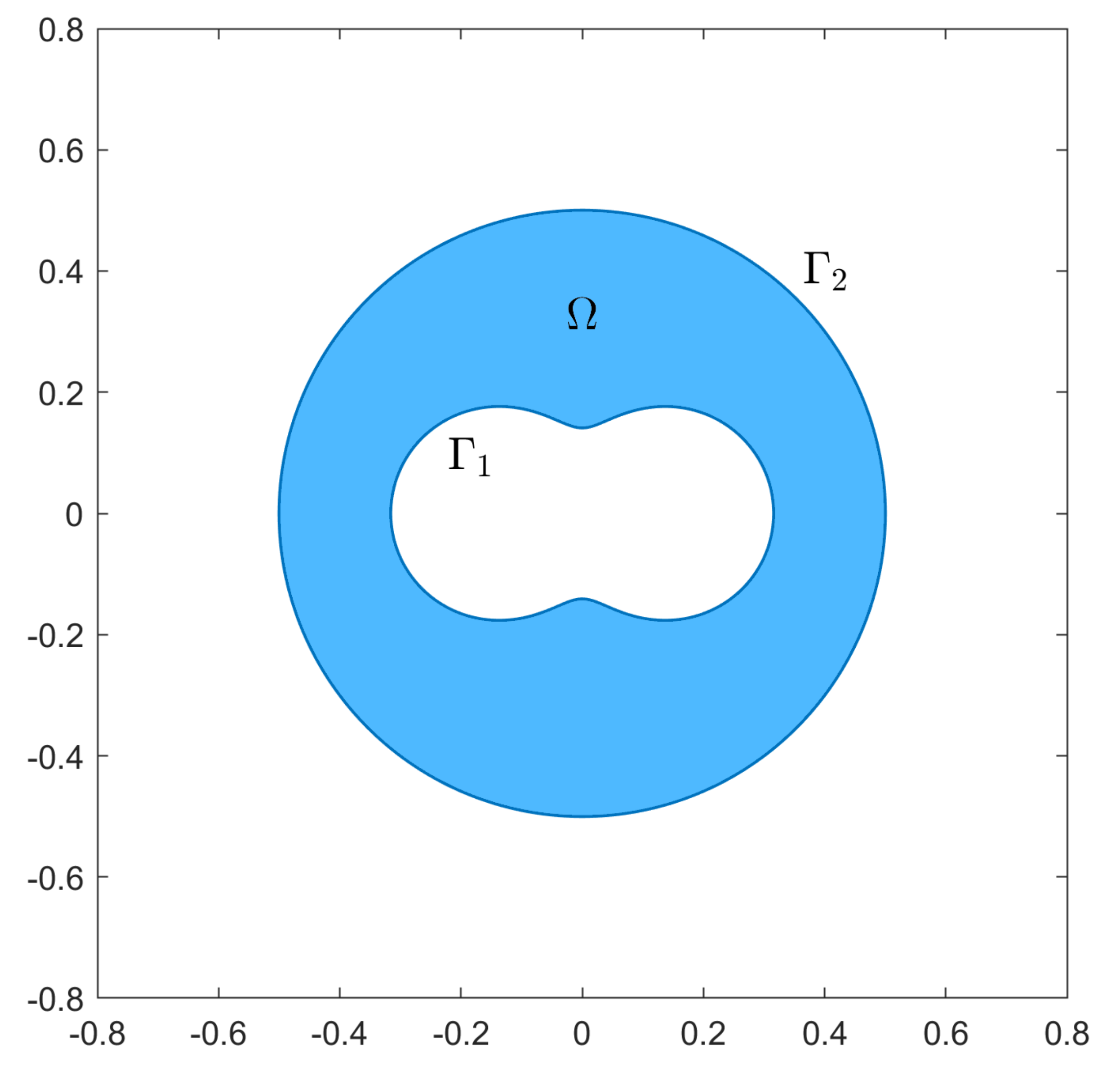
Problem formulation The domain $\mathrm{\Omega }$ is doubly connected in ${\mathrm{I}\mathrm{R}}^2$ with smooth boundary $\mathrm{\Gamma }$ of class $C^2.$ We assume that $\mathrm{\Gamma }$ consists of two disjoint curves ${\mathrm{\Gamma }}_1$ and ${\mathrm{\Gamma }}_2$, meaning $\mathrm{\Gamma }={\mathrm{\Gamma }}_1\cup {\mathrm{\Gamma }}_2,$ with ${\mathrm{\Gamma }}_1\cap {\Gamma }_2=\varnothing ,$ such that ${\mathrm{\Gamma }}_1$ is contained in the interior of ${\mathrm{\Gamma }}_2$ (see Figure 1).

Figure 1. The domain geometry and the notation used throughout this paper.

We consider the following initial boundary value problem for the wave equation

$$\frac{1}{a^2}\frac{{\partial }^{2}u}{\partial t^2}=\Delta u,\mathrm{in}\mathrm{\Omega }\times (0,\infty ),$$

(1)

subject to the homogeneous initial conditions

$$\frac{\partial u}{\partial t}(·,0)=u(·,0)=0, \text{in} \mathrm{\Omega }$$

(2)

and the boundary conditions

$$u=0,\text{on} {\Gamma }_1\times [0,\infty ),\text{and}\frac{\partial u}{\partial \nu }=g \text{on} {\mathrm{\Gamma }}_2\times [0,\infty ).$$

(3)

Here, $\Delta u=\frac{{\partial }^{2}u}{\partial x_1^2}+\frac{{\partial }^{2}u}{\partial x_2^2},$ for $x=(x_1,x_2)$, a represents the wave speed, $\nu$ denotes the outward unit normal vector to $\mathrm{\Gamma }$, and g is a given and sufficiently smooth function. We refer to [16] for the well-posedness of the direct problem to find the solution given the domain and the flux g.

In this work, we are interested in the numerical solution of the inverse problem to determine the interior boundary curve ${\mathrm{\Gamma }}_1$ from the knowledge of the Cauchy data on the exterior boundary ${\mathrm{\Gamma }}_2,$ meaning given g and

$$u=f,\text{on} {\mathrm{\Gamma }}_2\times (0,\infty ).$$

(4)

We note here that the formulated inverse problem can be interpreted as an optimization problem and can be solved using shape optimization tools [17].

An outline of the paper is as follows: in Section 2, we describe the combination of the Fourier–Laguerre transform with the non-linear boundary integral equation method for the hyperbolic inverse boundary problem. We derive a sequence of systems of non-linear boundary integral equations, which are transformed into $2\pi$-periodic integral equations. Then, we present an iterative scheme to recover the unknown boundary shape.

In Section 3, we discuss the numerical implementation of the proposed scheme. Given an initial approximation of the unknown boundary curve, we solve the system of equations on the boundary using a quadrature method. The correction of the boundary of the cavity is the solution of the linearized integral equation on the exterior boundary, which we discretize with a trigonometrical collocation method. The Tikhonov regularization is applied to the derived system of linear equations.

Numerical results are presented in Section 4, confirming that the outlined approach is a feasible way of reconstructing the boundary shape of a cavity.

2. A Two-Step Approach for Dimension Reduction

We first describe the solution u of (1)–(4) using a scaled Fourier expansion with respect to the Laguerre polynomials. Then, we represent the solution of the stationary problem using a single-layer ansatz.

2.1. Semi-Discretization in Time

We consider the expansion

$$u(x,t)=\kappa \sum _{n=0}^{\infty }{u}_n\left(x\right)L_n\left(\kappa t\right),$$

where

$$u_n\left(x\right)={\int }_0^{\infty }{e}^{-\kappa t}{L}_n\left(\kappa t\right)u(x,t)dt,n=0,1,2,\dots$$

for $\kappa >0,$ using the Laguerre polynomials $L_n$ of order n.

It is easy to show (see for example [15,18]) that u (sufficiently smooth) is the solution of the time-dependent problem (1)–(4) if and only if its Fourier–Laguerre coefficients $u_n$ satisfy the following sequence of mixed problems

$$\Delta u_n-{\gamma }^2{u}_n=\sum _{m=0}^{n-1}{\beta }_{n-m}{u}_m,\text{in} \mathrm{\Omega },$$

(5)

with boundary conditions

$$u_n=0,\mathrm{on} {\mathrm{\Gamma }}_1\mathrm{and}{u}_n=f_n,\frac{\partial u_n}{\partial \nu }=g_n,\text{on}{\mathrm{\Gamma }}_2.$$

(6)

Here ${\beta }_k=(k+1){\kappa }^2/a^2$, ${\gamma }^2={\beta }_0$ and

$$\begin{array}{cc}\hfill f_n\left(x\right)& ={\int }_0^{\infty }{e}^{-\kappa t}{L}_n\left(\kappa t\right)f(x,t)dt,n=0,1,2,\dots ,\hfill \\ \hfill g_n\left(x\right)& ={\int }_0^{\infty }{e}^{-\kappa t}{L}_n\left(\kappa t\right)g(x,t)dt,n=0,1,2,\dots .\hfill \end{array}$$

In order to apply the non-linear integral equation method, we need the sequence of fundamental solutions of Equation (5).

Definition 1.

The sequence of functions ${\mathrm{\Phi }}_n$, for $n=0,1,\dots$ is called the fundamental solution for the sequence of Equation (5) if it satisfies

$${\Delta }_x{\mathrm{\Phi }}_n(x,y)-\sum _{m=0}^n{\beta }_{n-m}{\mathrm{\Phi }}_m(x,y)=-\delta \left(\right|x-y\left|\right).$$

(7)

We consider the modified Bessel functions

$$I_0\left(z\right)=\sum _{n=0}^{\infty }\frac{1}{{(n!)}^2}{\left(\frac{z}{2}\right)}^{2n},I_1\left(z\right)=\sum _{n=0}^{\infty }\frac{1}{n!(n+1)!}{\left(\frac{z}{2}\right)}^{2n+1}$$

(8)

and the modified Hankel functions

$$\begin{array}{cc}\hfill K_0\left(z\right)& =-\left(ln\frac{z}{2}+C\right)I_0\left(z\right)+\sum _{n=1}^{\infty }\frac{\psi \left(n\right)}{{(n!)}^2}{\left(\frac{z}{2}\right)}^{2n},\hfill \\ \hfill K_1\left(z\right)& =\frac{1}{z}+\left(ln\frac{z}{2}+C\right)I_1\left(z\right)-\frac{1}{2}\sum _{n=0}^{\infty }\frac{\psi (n+1)+\psi \left(n\right)}{n!(n+1)!}{\left(\frac{z}{2}\right)}^{2n+1}\hfill \end{array}$$

(9)

of order zero and one, respectively. Here, we set $\psi \left(0\right)=0$ and

$$\psi \left(n\right)=\sum _{m=1}^n\frac{1}{m},n=1,2,\dots$$

and $C=0.57721\dots$ denotes the Euler constant [19]. We define the polynomials $v_n$ and $w_n$ by

$$v_n\left(r\right)=\sum _{k=0}^{\left[\frac{n}{2}\right]}{a}_{n,2k}{r}^{2k},w_n\left(r\right)=\sum _{k=0}^{\left[\frac{n-1}{2}\right]}{a}_{n,2k+1}{r}^{2k+1},$$

with the convention $w_0\left(r\right)=0.$ The coefficients are given by the relations

$$\begin{array}{cc}\hfill a_{n,0}& =1,\hfill \\ \hfill a_{n,n}& =-\frac{1}{2\gamma n}{\beta }_1{a}_{n-1,n-1},\hfill \\ \hfill a_{n,k}& =\frac{1}{2\gamma k}\left\{4{\left[\frac{k+1}{2}\right]}^2{a}_{n,k+1}-\sum _{m=k-1}^{n-1}{\beta }_{n-m}{a}_{m,k-1}\right\},k=n-1,\dots ,1,\hfill \end{array}$$

for $n=1,2,\dots$.

Then, following [18], we see that the sequence of functions

$${\mathrm{\Phi }}_n(x,y)=K_0\left(\gamma \right|x-y\left|\right)v_n\left(\right|x-y\left|\right)+K_1\left(\gamma \right|x-y\left|\right)w_n\left(\right|x-y\left|\right),x\ne y,$$

(10)

is a fundamental solution of (5) in a sense of Section 1.

2.2. A Boundary Integral Equation Method

A modified single-layer approach is proposed to solve the sequence of stationary problems. We represent the solutions $u_n$ of the problem (5) and (6) in the doubly-connected domain $\mathrm{\Omega }$ using the following single layer potential form

$$u_n\left(x\right)=\frac{1}{\pi }\sum _{\ell =1}^2\sum _{m=0}^n{\int }_{{\Gamma }_{\ell }}{\varphi }_m^{\ell }\left(y\right){\mathrm{\Phi }}_{n-m}(x,y)ds\left(y\right),x\in \Omega ,$$

(11)

with the unknown densities ${\varphi }_m^1$ and ${\varphi }_m^2$, $m=0,1,\dots$, defined on the boundary curves ${\mathrm{\Gamma }}_1$ and ${\mathrm{\Gamma }}_2$, respectively, and ${\mathrm{\Phi }}_n$ is given by (10).

We let x tend to the boundary $\mathrm{\Gamma }$ and, using the boundary conditions (6) and the standard jump relations, we obtain the following system of equations:

$$\begin{array}{cccc}\hfill \frac{1}{\pi }\sum _{\ell =1}^2{\int }_{{\mathrm{\Gamma }}_{\ell }}{\mathrm{\varphi }}_n^{\ell }\left(y\right){\mathrm{\Phi }}_0(x,y)ds\left(y\right)& =F_{1,n}\left(x\right),\hfill & & x\in {\mathrm{\Gamma }}_1,\hfill \end{array}$$

(12)

$$\begin{array}{cccc}\hfill {\varphi }_n^2\left(x\right)+\frac{1}{\pi }\sum _{\ell =1}^2{\int }_{{\mathrm{\Gamma }}_{\ell }}{\varphi }_n^{\ell }\left(y\right)\frac{\partial {\mathrm{\Phi }}_0}{\partial \nu \left(x\right)}(x,y)ds\left(y\right)& =G_n\left(x\right),\hfill & & x\in {\mathrm{\Gamma }}_2,\hfill \end{array}$$

(13)

$$\begin{array}{cccc}\hfill \frac{1}{\pi }\sum _{\ell =1}^2{\int }_{{\mathrm{\Gamma }}_{\ell }}{\varphi }_n^{\ell }\left(y\right){\mathrm{\Phi }}_0(x,y)ds\left(y\right)& =F_{2,n}\left(x\right),\hfill & & x\in {\mathrm{\Gamma }}_2,\hfill \end{array}$$

(14)

for the right-hand sides

$$\begin{array}{cc}\hfill F_{1,n}\left(x\right)& =-\frac{1}{\pi }\sum _{\ell =1}^2\sum _{m=0}^{n-1}{\int }_{{\mathrm{\Gamma }}_{\ell }}{\varphi }_m^{\ell }\left(y\right){\mathrm{\Phi }}_{n-m}(x,y)ds\left(y\right),\hfill \\ \hfill G_n\left(x\right)& =g_n\left(x\right)-\sum _{m=0}^{n-1}{\varphi }_m^2\left(x\right)-\frac{1}{\pi }\sum _{\ell =1}^2\sum _{m=0}^{n-1}{\int }_{{\mathrm{\Gamma }}_{\ell }}{\varphi }_m^{\ell }\left(y\right)\frac{\partial {\mathrm{\Phi }}_{n-m}}{\partial \nu \left(x\right)}(x,y)ds\left(y\right),\hfill \\ \hfill F_{2,n}\left(x\right)& =f_n\left(x\right)-\frac{1}{\pi }\sum _{\ell =1}^2\sum _{m=0}^{n-1}{\int }_{{\mathrm{\Gamma }}_{\ell }}{\varphi }_m^{\ell }\left(y\right){\mathrm{\Phi }}_{n-m}(x,y)ds\left(y\right).\hfill \end{array}$$

This is a system of three equations for the three unknowns: the two densities ${\varphi }_n^1,{\varphi }_n^2$ and the boundary curve ${\mathrm{\Gamma }}_1.$ The integral operators are singular and linear on the densities but act non-linearly on the boundary curve. We consider the Fréchet derivative of the integral operators for linearizing them.

Before presenting the iterative method, we consider the parametrization of the system (12)–(14). We assume the following parametric representation of the boundary

$${\mathrm{\Gamma }}_{\ell }=\{x_{\ell }\left(s\right)=(x_{1\ell }\left(s\right),x_{2\ell }\left(s\right)),s\in [0,2\pi ]\},\ell =1,2$$

and we define ${\phi }_n^{\ell }\left(s\right)={\varphi }_n^{\ell }\left(x_{\ell }\left(s\right)\right)\left|x_{\ell }^{\prime }\left(s\right)\right|.$

Then, the system (12)–(14) takes the form

$$\begin{array}{cccc}\hfill \frac{1}{2\pi }\sum _{\ell =1}^2{\int }_0^{2\pi }{\phi }_n^{\ell }\left(\sigma \right)H_0^{1,\ell }(s,\sigma )d\sigma & ={\tilde{F}}_{1,n}\left(s\right),\hfill & & s\in [0,2\pi ],\hfill \end{array}$$

(15)

$$\begin{array}{cccc}\hfill \frac{{\phi }_n^2\left(s\right)}{|x_2^{\prime }\left(s\right)|}+\frac{1}{2\pi }\sum _{\ell =1}^2{\int }_0^{2\pi }{\phi }_n^{\ell }\left(\sigma \right)Q_0^{2,\ell }(s,\sigma )d\sigma & ={\tilde{G}}_n\left(s\right),\hfill & & s\in [0,2\pi ],\hfill \end{array}$$

(16)

$$\begin{array}{cccc}\hfill \frac{1}{2\pi }\sum _{\ell =1}^2{\int }_0^{2\pi }{\phi }_n^{\ell }\left(\sigma \right)H_0^{2,\ell }(s,\sigma )d\sigma & ={\tilde{F}}_{2,n}\left(s\right),\hfill & & s\in [0,2\pi ],\hfill \end{array}$$

(17)

for $n=0,\dots ,N$, $N\in \mathrm{I}\mathrm{N},$ with the right-hand sides

$$\begin{array}{cc}\hfill {\tilde{F}}_{1,n}\left(s\right)& =-\frac{1}{2\pi }\sum _{\ell =1}^2\sum _{m=0}^{n-1}{\int }_0^{2\pi }{\phi }_m^{\ell }\left(\sigma \right)H_{n-m}^{1,\ell }(s,\sigma )d\sigma ,\hfill \\ \hfill {\tilde{G}}_n\left(s\right)& =g_n\left(x_2\left(s\right)\right)-\frac{1}{|x_2^{\prime }\left(s\right)|}\sum _{m=0}^{n-1}{\phi }_m^2\left(s\right)-\frac{1}{2\pi }\sum _{\ell =1}^2\sum _{m=0}^{n-1}{\int }_0^{2\pi }{\phi }_m^{\ell }\left(\sigma \right)Q_{n-m}^{2,\ell }(s,\sigma )d\sigma ,\hfill \\ \hfill {\tilde{F}}_{2,n}\left(s\right)& =f_n\left(x_2\left(s\right)\right)-\frac{1}{2\pi }\sum _{\ell =1}^2\sum _{m=0}^{n-1}{\int }_0^{2\pi }{\phi }_m^{\ell }\left(\sigma \right)H_{n-m}^{2,\ell }(s,\sigma )d\sigma .\hfill \end{array}$$

The kernels are given by

$$H_n^{k,\ell }(s,\sigma )=2{\mathrm{\Phi }}_n(x_k\left(s\right),x_{\ell }\left(\sigma \right)),Q_n^{k,\ell }(s,\sigma )=2\frac{\partial {\mathrm{\Phi }}_n}{\partial \nu \left(x\right)}(x_k\left(s\right),x_{\ell }\left(\sigma \right)),$$

(18)

for $s\ne \sigma ,k,\ell =1,2$, and $n=0,\dots ,N$. The functions ${\mathrm{\Phi }}_n$ are defined in (10).

2.3. The Iterative Scheme

We solve the derived systems of equations iteratively by splitting them to their well- and ill-posed parts. Following [20], we first solve the well-posed subsystem to obtain the corresponding densities and then we linearize (with respect to the boundary) the ill-posed subsystem to be solved for the update of the radial function.

In the following, we assume for simplicity a star-like interior curve with parametrization

$$x_1\left(s\right)=\{r\left(s\right)(coss,sins):s\in [0,2\pi ]\},$$

(19)

where $r:\mathrm{I}\mathrm{R}\to (0,\infty )$ is a $2\pi -$periodic function representing the radial distance from the origin.

We propose to solve the system of Equations (15)–(17) using the iterative scheme:

Step 1.

Given an initial approximation of ${\mathrm{\Gamma }}_1$, we solve the sequence of well-posed systems of integral Equations (15) and (17) for ${\phi }_n^1,{\phi }_n^2,n=0,...,N.$

Step 2

Keeping now the densities fixed, we linearize the ill-posed integral Equation (17) resulting to

$$\sum _{m=0}^n{\mathcal{D}}_{n-m}[{\phi }_m^1,r;q]\left(s\right)=f_n\left(x_2\left(s\right)\right)-\frac{1}{2\pi }\sum _{\ell =1}^2\sum _{m=0}^n{\int }_0^{2\pi }{\phi }_m^{\ell }\left(\sigma \right)H_{n-m}^{2,\ell }(s,\sigma )d\sigma ,$$

(20)

where q is the radial function of the perturbed boundary. We solve the N equations for the radial function q of the perturbed ${\mathrm{\Gamma }}_1,$ and we update as $r+q.$

Equation (20) contains the Fréchet derivative ${\mathcal{D}}_n$ of the integral operator with kernel $H_n^{2,\ell }$ with respect to $x_1.$ This is a linear operator on q, and its form is obtained by the formal differentiation of the kernel $H_n^{2,\ell }$ with respect to $x_1.$ We get

$${\mathcal{D}}_n[\phi ,r;q]\left(s\right)=\frac{1}{2\pi }{\int }_0^{2\pi }q\left(\sigma \right)\phi \left(\sigma \right)D_n(s,\sigma )d\sigma ,$$

with kernel

$$D_n(s,\sigma )=-\frac{(x_2\left(s\right)-x_1\left(\sigma \right))·(cos\sigma ,sin\sigma )}{|x_2\left(s\right)-x_1\left(\sigma \right)|}{\tilde{\mathrm{\Phi }}}_n\left(\right|x_2\left(s\right)-x_1\left(\sigma \right)\left|\right),$$

where

$${\tilde{\mathrm{\Phi }}}_n\left(r\right)=K_1\left(\gamma r\right){\tilde{v}}_n\left(r\right)+K_0\left(\gamma r\right){\tilde{w}}_n\left(r\right),$$

for the polynomials

$$\begin{array}{cc}\hfill {\tilde{v}}_n\left(r\right)& =\gamma \sum _{m=0}^{\left[\frac{n}{2}\right]}{a}_{n,2m}{r}^{2m}-2\sum _{m=1}^{\left[\frac{n-1}{2}\right]}m{a}_{n,2m+1}{r}^{2m},\hfill \\ \hfill {\tilde{w}}_n\left(r\right)& =\gamma \sum _{m=0}^{\left[\frac{n-1}{2}\right]}{a}_{n,2m+1}{r}^{2m+1}-2\sum _{m=1}^{\left[\frac{n}{2}\right]}m{a}_{n,2m}{r}^{2m-1}.\hfill \end{array}$$

Note that the Fréchet derivative operator ${\mathcal{D}}_n[\tilde{\phi },r;q]$ is injective at the exact solution [15].

3. Numerical Implementation

The numerical implementation of the iterative scheme has been well examined in [15] for a system similar to (15)–(17). Thus, in this section, we give just a brief description of it. We refer to (15) as the “field” equations and to (16) as the “data” equations.

With the given current approximation of the interior boundary ${\Gamma }_1$, we consider the “field” Equation (15). Firstly, we handle the singularity of the parametrized kernels. More precisely, the kernel $H_n^{\ell ,\ell }$ in (18) admits logarithmic singularity. After lengthy but straightforward calculations, we derive the following decomposition:

$$H_n^{\ell ,\ell }(s,\sigma )=H_{n,1}^{\ell ,\ell }(s,\sigma )ln\left(\frac{4}{e}{sin}^2\frac{s-\sigma }{2}\right)+H_{n,2}^{\ell ,\ell }(s,\sigma ),$$

where

$$\begin{array}{ccc}\hfill H_{n,1}^{\ell ,\ell }(s,\sigma )& =& -I_0\left(\gamma \right|x_{\ell }\left(s\right)-x_{\ell }\left(\sigma \right)\left|\right)v_n\left(\right|x_{\ell }\left(s\right)-x_{\ell }\left(\sigma \right)\left|\right)\hfill \\ \\ & & +I_1\left(\gamma \right|x_{\ell }\left(s\right)-x_{\ell }\left(\sigma \right)\left|\right)w_n\left(\right|x_{\ell }\left(s\right)-x_{\ell }\left(\sigma \right)\left|\right)\hfill \end{array}$$

(21)

and

$$H_{n,2}^{\ell ,\ell }(s,\sigma )=H_n^{\ell ,\ell }(s,\sigma )-H_{n,1}^{\ell ,\ell }(s,\sigma )ln\left(\frac{4}{e}{sin}^2\frac{s-\sigma }{2}\right)$$

with diagonal terms

$$H_{n,2}^{\ell ,\ell }(s,s)=-2C-1-2ln\left(\frac{\gamma |x_{\ell }^{\prime }\left(s\right)|}{2}\right)+\frac{2a_{n,1}}{\gamma },n=0,1,2,\dots ,N.$$

Furthermore, the kernels $Q_{\ell ,\ell }^n$ have logarithmic singularities

$$Q_n^{\ell ,\ell }(s,\sigma )=Q_{n,1}^{\ell ,\ell }(s,\sigma )ln\left(\frac{4}{e}{sin}^2\frac{s-\sigma }{2}\right)+Q_{n,2}^{\ell ,\ell }(s,\sigma ),$$

where

$$\begin{array}{ccc}\hfill Q_{n,1}^{\ell ,\ell }(s,\sigma )& =& h^{\ell ,\ell }(s,\sigma )\{I_1\left(\gamma \right|x_{\ell }\left(s\right)-x_k\left(\sigma \right)\left|\right){\tilde{v}}_n\left(\right|x_{\ell }\left(s\right)-x_k\left(\sigma \right)\left|\right)\hfill \\ \\ & & -I_0\left(\gamma \right|x_{\ell }\left(s\right)-x_k\left(\sigma \right)\left|\right){\tilde{w}}_n\left(\right|x_{\ell }\left(s\right)-x_k\left(\sigma \right)\left|\right)\}\hfill \end{array}$$

(22)

and

$$Q_{n,2}^{\ell ,\ell }(s,\sigma )=Q_{\ell ,\ell }^n(s,\sigma )-Q_{n,1}^{\ell ,\ell }(s,\sigma )ln\left(\frac{4}{e}{sin}^2\frac{s-\sigma }{2}\right)$$

with diagonal terms

$$Q_{n,2}^{\ell ,\ell }(s,s)=\frac{x_{\ell ,2}^{\prime }\left(s\right)x_{\ell ,1}^{\prime \prime }\left(s\right)-x_{\ell ,1}^{\prime }\left(s\right)x_{\ell ,2}^{\prime \prime }\left(s\right)}{|x_{\ell }^{\prime }{\left(s\right)|}^3},n=0,1,\dots ,N.$$

Here, we introduce the function

$$h^{\ell ,k}(s,\sigma )=\frac{(x_{\ell ,1}\left(s\right)-x_{k,1}\left(\sigma \right))x_{\ell ,2}^{\prime }\left(s\right)-(x_{2,\ell }\left(s\right)-x_{k,2}\left(\sigma \right))x_{\ell ,1}^{\prime }\left(s\right)}{|x_k\left(\sigma \right)-x_{\ell }\left(s\right)|}.$$

Clearly the kernels $H_n^{k,\ell }$ and $Q_n^{k,\ell }$ are smooth for $k\ne \ell$, $k,\ell =1,2$.

Thus, we have to solve the sequence of systems of well-posed $2\pi$ periodical integral Equation (15) with logarithmic singularities. We use for it the Nyström method with trigonometrical quadrature rules (see for details [15,21]).

For the “data” Equation (16), we apply the collocation method and, due to its ill-posedness, the received sequence of linear systems is solved by Tikhonov regularization.

4. Numerical Results

We approximate the function q by a trigonometric polynomial of the form

$$q\left(s\right)\approx \sum _{j=0}^{2J}{q}_j{\tau }_j\left(s\right),J\in \mathrm{I}\mathrm{N},$$

(23)

with

$${\tau }_j\left(s\right)=\left\{\begin{array}{cc}cos\left(js\right),\hfill & \mathrm{for}j=0,...,J,\hfill \\ sin\left(\right(j-J\left)s\right),\hfill & \mathrm{for}j=J+1,...,2J.\hfill \end{array}\right.$$

We substitute (23) in the linearized “data” equations and at the nodal points

$$s_k=\frac{k\pi }{M},k=0,\dots ,2M-1,M\in \mathrm{I}\mathrm{N},$$

we obtain a linear system of the form

$$\mathbf{A}\left(n\right)\mathbf{q}=\mathbf{b}\left(n\right),n=0,\dots ,N,$$

for the unknown coefficients $\mathbf{q}={(q_0,\dots ,q_{2J})}^{⊺}$, where $\mathbf{A}$ and $\mathbf{b}$ describe the left- and right-hand side of the linearized “data” equations, respectively.

The above equation is ill-posed, and thus we apply Tikhonov regularization

$$\underset{\mathbf{q}}{min}\left\{\right||\mathbf{A}\mathbf{q}-{\mathbf{b}\left|\right|}_2^2+{\lambda \left|\right|\mathbf{q}\left|\right|}_2^2\}.$$

The regularization parameter $\lambda >0$ is chosen initially by trail and error and decreases at every iteration step as

$${\lambda }_{\ell }={\lambda }_{0}0.9^{\ell -1},\ell =1,2,\dots .$$

This is a heuristic approach to compute $\lambda$ but provides satisfactory reconstructions, as we can see later. There exist more sophisticated techniques, but this investigation is out of the scope of this work.

We simulate the Cauchy data by solving the sequence (5) with boundary conditions

$$u_n=f_{1,n},\text{on} {\mathrm{\Gamma }}_1,\text{and}{u}_n=f_{2,n},\text{on}{\Gamma }_2,$$

for given boundary functions $f_{\ell ,n},\ell =1,2.$ To avoid an inverse problem, we consider double the amount of nodal points for the direct problem, and afterwards we add noise to the Cauchy data on the boundary ${\Gamma }_2$ with respect to the $L^2$ norm. We use the boundary functions

$$f_{1,n}=0,\mathrm{and}{f}_{2,n}=\frac{e(2+\kappa n(\kappa (n-1)-4\left)\right)}{4{(\kappa +1)}^{n+3}},n=0,...,N.$$

We consider two examples with different boundary curves:

Example 1.

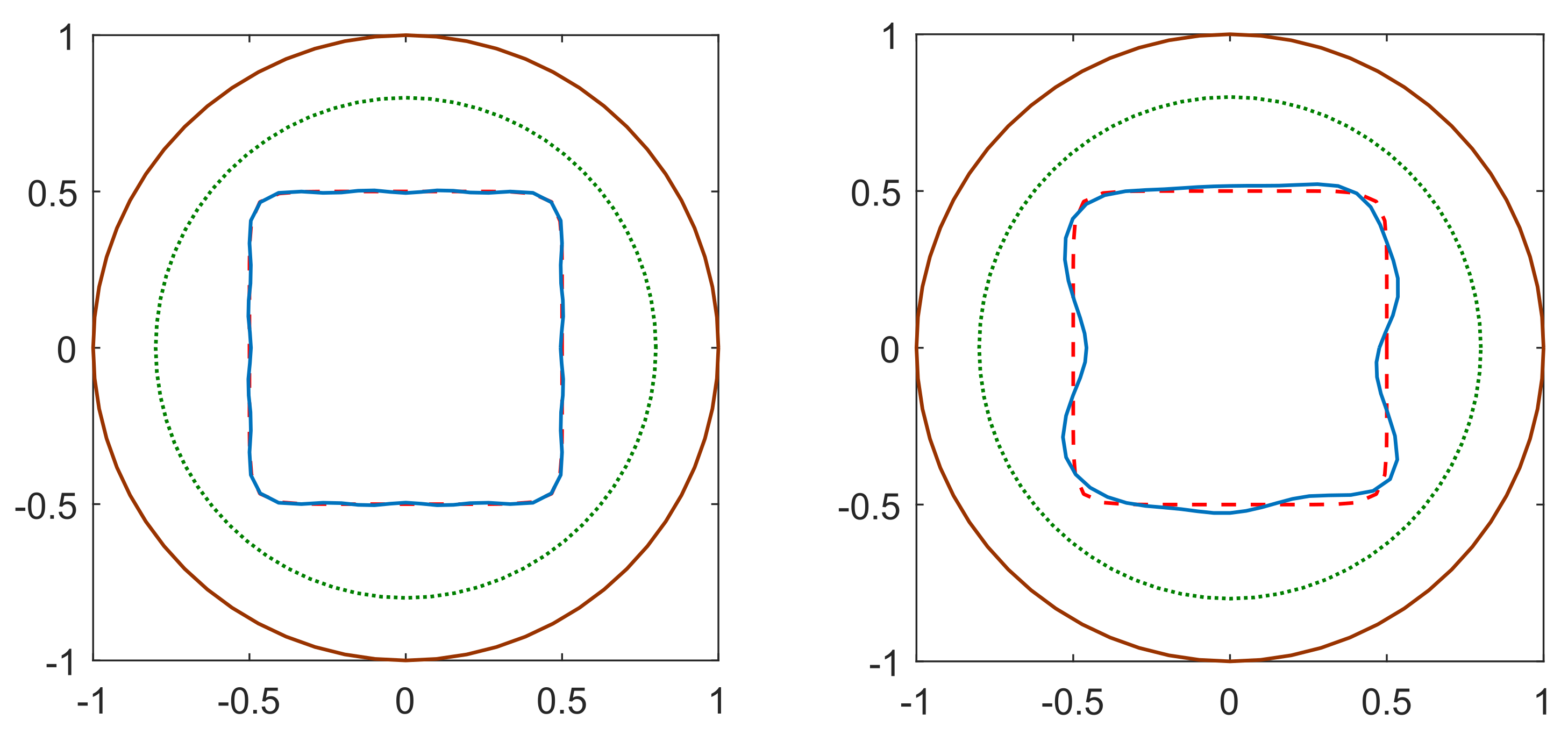
The interior boundary curve ${\mathrm{\Gamma }}_1$ is a rounded rectangle with radial function

$$r_1\left(s\right)={({cos}^{10}s+{sin}^{10}s)}^{-0.1}$$

and ${\mathrm{\Gamma }}_2$ is a circle with center $(0,0)$ and radius $1.$

Example 2.

Here, both boundary curves are apple-shaped with parametrizations

$$x_1\left(s\right)=r_1\left(s\right)(coss,sins),and{x}_2\left(s\right)=(r_2\left(s\right)coss-0.4,r_2\left(s\right)sins),$$

for the radial functions

$$r_1\left(s\right)=\frac{0.45+0.3coss-0.1sin2s}{1.2+0.9coss},and{r}_2\left(s\right)=\frac{1+0.9coss+0.1sin2s}{0.8+0.6coss}.$$

In both examples, the initial guess is a circle with center $(0,0)$ and radius $r_0.$ We set $\alpha =1$ and $\kappa =1,$ we use $N=10$ Fourier coefficients and we solve at the nodal points with $M=64.$ In the following figures, the brown solid line represents the boundary ${\mathrm{\Gamma }}_2,$ the green dotted line shows the initial guess, the red dashed line is the exact boundary ${\mathrm{\Gamma }}_1$ and its reconstruction is the blue solid line.

In the first example, the initial radius is given by $r_0=0.8$ and we use $J=13.$ In Figure 2, we see the reconstructions for exact (left) and noisy (right) data. The presented results are, with the initial regularization parameter ${\lambda }_0=0.01,$ after 21 and 12 iterations, respectively.

Figure 2. Reconstructions of the boundary ${\mathrm{\Gamma }}_1$ of the rounded rectangle for exact data (left) and data with $3\%$ noise (right).

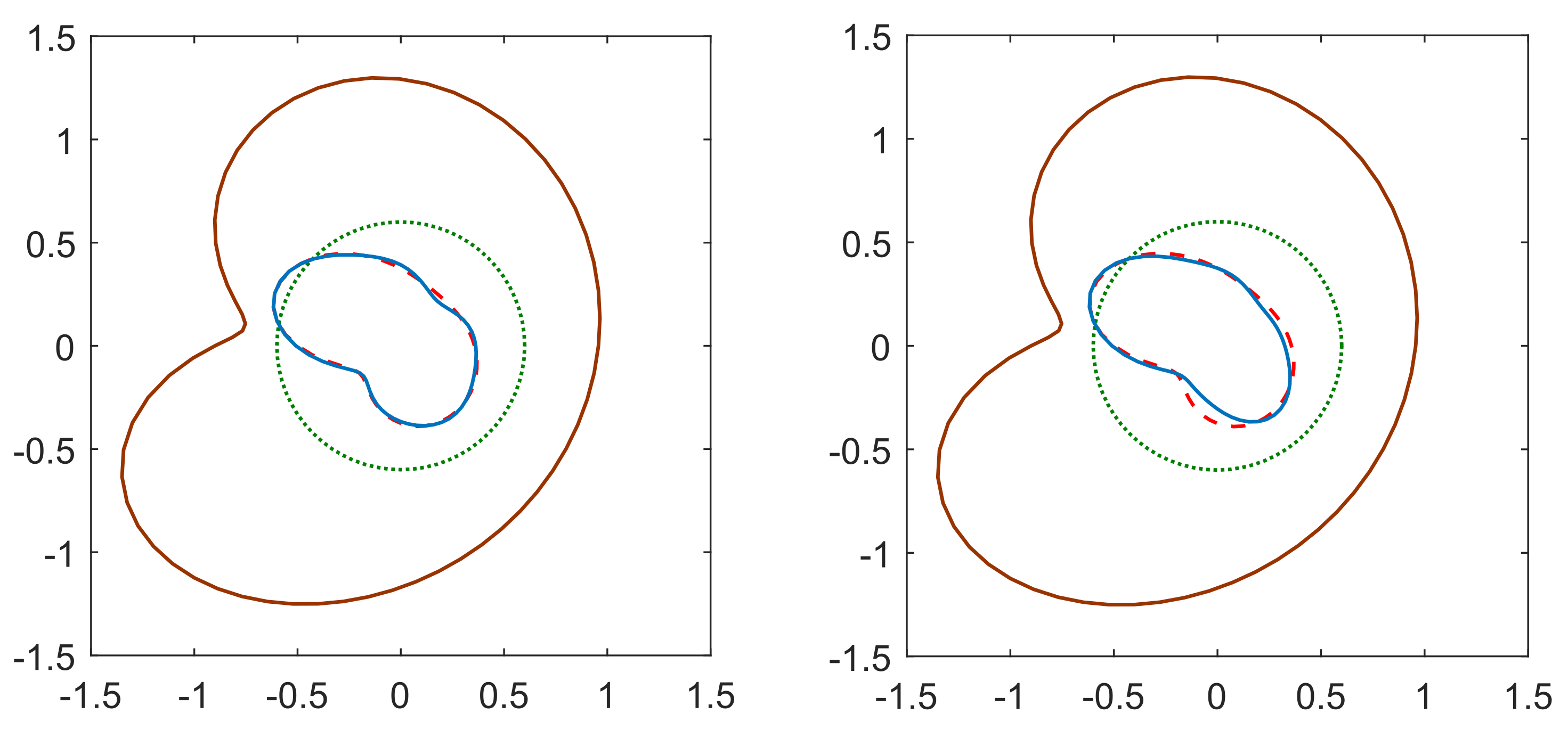
For the second example, we set $J=5$ and $r_0=0.6.$ We consider ${\lambda }_0=0.001$ for the reconstructions presented in Figure 3. The algorithm terminated after 10 and 7 iterations, for the noise-free and noisy data, respectively.

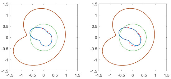
Figure 3. Reconstructions of theapple-shaped boundary ${\mathrm{\Gamma }}_1$ for exact data (left) and data with $3\%$ noise (right).

We observe that we obtain accurate and relative stable reconstructions of the boundary curve. However, we have to stress that the results are sensitive with respect to the initial guess.

5. Conclusions

We extended the integral equation method to the inverse hyperbolic problem of the reconstruction of the interior boundary curve given the Cauchy data on the exterior boundary of a doubly connected planar domain. We applied the Laguerre transform in time, and we derived a sequence of stationary inverse boundary problems. These problems were reduced to a sequence of non-linear boundary integral equations by the application of modified single layer potentials. The Nyström method is used for the well-posed system of linear integral equations, and the collocation method together with Tikhonov regularization is applied to the the ill-posed sub-system. This technique can be extended to the case of three-dimensional domains for similar but more involved fundamental sequences.

References

- Cakoni, F.; Haddar, H. Analysis of two linear sampling methods applied to electromagnetic imaging of buried objects. Inverse Probl. 2006, 22, 845. [Google Scholar] [CrossRef] [Green Version]
- Caorsi, S.; Massa, A.; Pastorino, M.; Raffetto, M.; Randazzo, A. Detection of buried inhomogeneous elliptic cylinders by a memetic algorithm. IEEE Trans. Antennas Propag. 2003, 51, 2878–2884. [Google Scholar] [CrossRef]
- Massa, A.; Pastorino, M.; Randazzo, A. Reconstruction of two-dimensional buried objects by a differential evolution method. Inverse Probl. 2004, 20, S135–S150. [Google Scholar] [CrossRef]
- Naik, N.; Eriksson, J.; de Groen, P.; Sahli, H. A nonlinear iterative reconstruction and analysis approach to shape-based approximate electromagnetic tomography. IEEE Trans. Geosci. Remote Sens. 2008, 46, 1558–1574. [Google Scholar] [CrossRef]
- Alves, C.J.S.; Kress, R.; Silvestre, A.L. Integral equations for an inverse boundary value problem for the two-dimensional Stokes equations. J. Inverse Ill-Posed Probl. 2007, 15, 461–481. [Google Scholar] [CrossRef]
- Cakoni, F.; Cristo, M.D.; Sun, J. A multistep reciprocity gap functional method for the inverse problem in a multilayered medium. Complex Var. Elliptic Equ. 2012, 57, 261–276. [Google Scholar] [CrossRef]
- Kress, R.; Rundell, W. Nonlinear integral equations and the iterative solution for an inverse boundary value problem. Inverse Probl. 2005, 21, 1207–1223. [Google Scholar] [CrossRef]
- Chapko, R.; Gintides, D.; Mindrinos, L. The inverse scattering problem by an elastic inclusion. Adv. Comput. Math. 2018, 44, 453–476. [Google Scholar] [CrossRef] [Green Version]
- Chapko, R.; Ivanyshyn, Y.O.; Kanafotskyi, T.S. On the non-linear integral equation approaches for the boundary reconstruction in double-connected planar domains. J. Numer. Appl. Math. 2016, 122, 7–20. [Google Scholar]
- Gintides, D.; Mindrinos, L. The inverse electromagnetic scattering problem by a penetrable cylinder at oblique incidence. Appl. Anal. 2019, 98, 781–798. [Google Scholar] [CrossRef] [Green Version]
- Colton, D.; Kress, R. Inverse Acoustic and Electromagnetic Scattering Theory; Springer: Berlin, Germany, 2013. [Google Scholar]
- Chapko, R.; Kress, R.; Yoon, J.R. On the numerical solution of an inverse boundary value problem for the heat equation. Inverse Probl. 1998, 14, 853. [Google Scholar] [CrossRef]
- Halbrecht, H.; Tausch, J. On the numerical solution of a shape optimization problem for the heat equation. SIAM J. Sci. Comput. 2013, 35, A104–A121. [Google Scholar] [CrossRef] [Green Version]
- Wang, H.; Li, Y. Numerical solution of an inverse boundary value problem for the heat equation with unknown inclusions. J. Comput. Phys. 2018, 369, 1–15. [Google Scholar] [CrossRef]
- Chapko, R.; Mindrinos, L. On the non-linear integral equation approach for an inverse boundary value problem for the heat equation. J. Eng. Math. 2019, 119, 255–268. [Google Scholar] [CrossRef] [Green Version]
- Lions, J.L.; Magenes, E. Non-Homogeneous Boundary Value Problems and Applications I; Springer: Berlin, Germany, 1972. [Google Scholar]
- Ndiaye, F.; Ly, I. Inverse problem related to boundary shape identification for a hyperbolic differential equation. Int. J. Math. Math. Sci. 2021, 2021, 1716027. [Google Scholar] [CrossRef]
- Chapko, R.; Kress, R. On the numerical solution of initial boundary value problems by the Laguerre transformation and boundary integral equations. In Integral and Integrodifferential Equations: Theory, Methods and Applications. Series in Mathematical Analysis and Applications; Agarwal, R.P., O’Regan, D., Eds.; Gordon and Breach Science Publishers: Amsterdam, The Netherlands, 2000; Volume 2, pp. 55–69. [Google Scholar]
- Abramowitz, M.; Stegun, I.A. Handbook of Mathematical Functions with Formulas, Graphs, and Mathematical Tables; National Bureau of Standards Applied Mathematics Series; Government Printing Office: Washington, DC, USA, 1972. [Google Scholar]
- Johansson, B.T.; Sleeman, B.D. Reconstruction of an acoustically sound-soft obstacle from one incident field and the far-field pattern. IMA J. Appl. Math. 2007, 72, 96–112. [Google Scholar] [CrossRef]
- Kress, R. Linear Integral Equations; Springer: Berlin, Germany, 2014. [Google Scholar]
Publisher’s Note: MDPI stays neutral with regard to jurisdictional claims in published maps and institutional affiliations. |
© 2022 by the authors. Licensee MDPI, Basel, Switzerland. This article is an open access article distributed under the terms and conditions of the Creative Commons Attribution (CC BY) license (https://creativecommons.org/licenses/by/4.0/).