Abstract
The current work aims to develop an approximation of the slice of a Minkowski sum of finite number of ellipsoids, sliced up by an arbitrarily oriented plane in Euclidean space that, to the best of the author’s knowledge, has not been addressed yet. This approximation of the actual slice is in a closed form of an explicit parametric equation in the case that the slice is not passing through the zones of the Minkowski surface with high curvatures, namely the “corners”. An alternative computational algorithm is introduced for the cases that the plane slices the corners, in which a family of ellipsoidal inner and outer bounds of the Minkowski sum is used to construct a “narrow strip” for the actual slice of Minkowski sum. This strip can narrow persistently for a few more number of constructing bounds to precisely coincide on the actual slice of Minkowski sum. This algorithm is also applicable to the cases with high aspect ratio of ellipsoids. In line with the main goal, some ellipsoidal inner and outer bounds and approximations are discussed, including the so-called “Kurzhanski’s” bounds, which can be used to formulate the approximation of the slice of Minkowski sum.
Keywords:
slice of Minkowski sum; ellipsoids; closed-form parametrization; approximation; computational algorithm; Kurzhanski’s bounds MSC:
00A06
1. Introduction
The Minkowski sum is a binary operator between two sets of position vectors in n-dimensional Euclidean space , which defines a way to add up the two sets and generate a new set of points with a different geometry. This operator is commutative and associative and allows successive implementation of that to the countable (more practically finite) number of the sets. Let and be two sets of vectors, then the Minkowski sum is defined by vector addition of every vector with every vector
This is equivalent to define the Minkowski sum as the set of all translated copies of set by every translation vector
From (2), one can easily imagine that the Minkowski sum of a geometrical shape (object) and a point is the translated shape by the position vector of that point and, similarly, the sum of an object and a curve is that object moving along the curve. The concepts of Minkowski sum and slice of Minkowski sum are widely used in vast areas of engineering, such as robot motion planing [1,2], computer-aided design [3], assembly planning [4] and especially crystallography [5,6]. In crystallography, X-ray diffraction is an experimental technique to determine the atomic and molecular structure of a crystalline material, that is to figure out the orientation and position of each atom or molecule within a unit cell of the crystal. The unit cell is the smallest building unit of the crystalline material that inherits the symmetry of the crystal, such that the entire crystal is constructed from repeating this unit. The X-ray diffraction experiment does not provide full information about the electron density within a unit cell, which is required to determine the crystal structure. It measures the magnitude of the Fourier transform of the electron density of the entire molecular contents in a unit cell. In order to apply the inverse of Fourier transform to compute the electron density function in Euclidean space, the phase information is required that is not provided from measurement of X-ray diffraction. Therefore, molecular replacement (MR) was developed as a computational technique in the 1960s [7] to complement the X-ray experimental data. The idea of MR is to search first for the orientation of each molecule within a unit cell of crystal over the Lie group of spacial orthogonal matrices, followed by a search for the position of that molecule over the unit cell, which is computationally a heavy search. Chirikjian et al. [8,9,10,11] developed the concept of motion space through a series of papers, which shrinks the feasible search space in MR to a subset (fundamental domain) , where and the symmetry group of the crystal is a discrete subgroup of . The denotes the Lie group of special Euclidean transformation of matrices, which is defined as the semi-direct product of Lie group acting on vector space (also group) . Shiffman et al. [5] continued to work on the feasible motion space and used the concept of slice of Minkowski sum to reduce the size of the feasible search space in MR technique. They used the concept of moment-of-inertia ellipsoid to approximate the protein macromolecules with ellipsoids. Then, they discussed that in order for the packing ellipsoids to form a rigid crystal, the ellipsoids should not interpenetrate (collide) but should be in contact with enough number of neighbors. They determined the collision zone, which must be excluded from the searching motion space in MR and showed that the remaining feasible search space is small. They constructed the collision zone as the intersection of the fundamental domain with a slice of Minkowski sum of ellipsoids.
One can show that the Minkowski sum of two convex sets is a convex set. This fact allows to define the configuration space obstacle in robotic motion planning. Assuming a robot that can move in three-dimensional Euclidean space , the configuration-free space of the robot is defined as the set of all positions in space that the robot can inhabit. Conversely, the configuration space obstacle is described as the set of all positions in configuration space that the robot cannot attain due to collision with existing fixed obstacles. The geometry and position of the configuration space obstacle depend on geometries and positions of both the obstacle and the robot. Let be the set of all points of an obstacle and represent the set of points that describes a robot, then the configuration space obstacle is mathematically determined by Minkowski sum , where is the inverse of the set R with respect to an arbitrarily selected body-fixed reference frame on the robot R. In this computation, the coordinates of every point on robot R are measured with respect to the body-fixed reference frame on R, while the coordinates of points on the obstacle P and also the coordinates of the points in the Minkowski sum are measured with respect to the global frame of reference. The configuration of is geometrically determined by locating the boundary of robot R on the boundary of obstacle P and sweeping it along the boundary of P. In other words, the configuration space obstacle is described as the locus of the reference point on the robot R, measured in the global frame of reference, when the boundary of robot R is touching the boundary of obstacle P and sweeping along it. This is similar to interpreting the Minkowski sum as a deformed offset of the set P with variable offset distance. This deformed-offset interpretation was creatively used in [12] to suggest a closed-form parametric equation for the Minkowski sum of two ellipsoids. The novelty in that work is to use the fact that the affine transformation of an ellipsoid is an ellipsoid, possibly with different sizes of semi-axes and orientation, and also to use the concept of offset surface of an ellipsoid.
For the rest of this paper let for denote the so-called “solid ellipsoid” as the set of all points that satisfy the implicit relation . In this notation, is the center of ellipsoid , and is a symmetric positive definite matrix with real entries, which determines the size and orientation of the ellipsoid such that is the rotation matrix corresponding to the orientation of that ellipsoid, is the diagonal matrix with entries of the semi-axis length of the solid ellipsoid corresponding to the size of that ellipsoid, such that . Note that, here, denotes the set of all symmetric positive definite matrices with real entries, and is the special orthogonal group corresponding to [13,14,15]. Similarly, the ellipsoid is defined as the dimensional surface, which is embedded in and encloses the sold ellipsoid , that is . Note that, in the current work, both terms “solid ellipsoid” and “ellipsoid” might be used interchangeably, where the precise meaning is clear from the content. Furthermore, here, the word “ellipse” is used with its common meaning as a one-dimensional curve, embedded in for , while the word “ellipsoid” is also used to describe the one-dimensional ellipse, in general. Chirikjian et al. [16] reformed the closed-form formula of the Minkowski sum of two ellipsoids in [12] as:
where denotes the Euclidean norm, explicitly parametrizes the ellipsoid centered at and is the unit vector in that is parametrized by angles such that it describes the -dimensional surface of the unit sphere centered at the origin and embedded in . Note that in the Minkowski sum formula (3), the ellipsoid is centered at the origin so that the Minkowski sum also represents the configuration space obstacle of the two ellipsoids. This has many applications in robot motion planning, where the geometries of the robot and each obstacle are approximated by the enclosing ellipsoids, and then the configuration space obstacle is calculated as the Minkowski sum of two ellipsoids, when the robot ellipsoid is measured in the body-fixed frame of reference located on the center of the ellipsoid [1].
Recall that Minkowski sum is a commutative operator such that , however, the form of the equation in (3) does not imply the symmetry in formulation, such that for a particular angular parameter . Therefore, Chirikjian et al. [16] also reformulated a symmetric closed-form parametrization of the Minkowski sum that is more consistent with the commutative characteristic of the Minkowski sum operator. The advantage of this symmetric formula compared with the asymmetric (3) is that they could extend it to the Minkowski sum of countably finite number of ellipsoids (also see [17]):
where . As expected from the definition of the Minkowski sum in (1) and (2), the Minkowski sum of ellipsoids is not an ellipsoid. This fact is also inferred from (4), where the sum of the countably finite number of symmetric positive definite matrices returns a symmetric positive definite matrix, necessary for generating an ellipsoid, however, in this case, the formula (4) does not parametrize an ellipsoid, since the denominators are variable parametrized positive scalars, , rather than being fixed positive scalars. At the end, it is notable that in the literature the Minkowski sum of two ellipsoids was also studied numerically [18,19,20] or by calculus of ellipsoids [21,22,23].
For the rest of this paper, some ellipsoidal outer and inner bounds of the Minkowski sum are briefly reviewed, including the so-called “Kurzhanski’s” bounds. Furthermore, some ellipsoidal approximations are suggested for the Minkowski sum, which they do not necessarily bound the Minkowski sum from, neither inside nor outside; however, they are used later, as well as the inner and outer bounds, to derive a closed-form parametrization of the slice of Minkowski sum. This symmetric closed form is to approximate the slice of Minkowski sum in the case that the actual slice does not pass through the zones of the Minkowski surface with high curvature, namely the “corner” zones. Then, the results from model are compared with the actual slice of Minkowski sum for different ellipsoidal approximations and bounds. Finally, an alternative algorithm is introduced in the case that the actual slice passes closely through the corners of the Minkowski surface with high curvature, in which a family of ellipsoidal inner and outer bounds of the Minkowski sum is used to construct a “narrow strip” for the slice of Minkowski sum. This strip can narrow persistently for a few more numbers of constructing bounds to precisely coincide on the actual slice of Minkowski sum. The strip algorithm is also applied in the case of a slice of a Minkowski sum of ellipsoids with high aspect ratio.
2. Ellipsoidal Bounds and Ellipsoidal Approximations of Minkowski Sum of Ellipsoids
In this section, some ellipsoidal inner and outer bounds and ellipsoidal approximations of the Minkowski sum of ellipsoids are discussed. These bounds and approximations are later used in the following section to derive a closed-form equation of the slice of Minkowski sum.
Given a countably finite number of ellipsoids centered at the origin for , every solid ellipsoid defined by:
contains the Minkowski sum as an outer bound for such that [21,24,25]
Other suggestions for possible coefficients in (5) were introduced in [16]. Considering again the finite number of arbitrary ellipsoids for Kurzhanski et al. [21,26] presented a family of outer ellipsoidal bounds , centered at , where is parametrized by the unit vector . Similarly, but by different parametrization, Durieu et al. [24] suggested a family of outer bounds of the Minkowski sum of a finite number of ellipsoids. Compatible with (5), in the case of a Minkowski sum of two ellipsoids, a family of outer ellipsoidal bounds is parametrized by [21,27,28]
where and are the roots of the equation:
Halder [29] showed that, in the case of two ellipsoids, the parametrized matrix of the Kurzhanski’s outer bound in [21,26] is transformed into in (7). He also showed that, similarly but by a different transformation, the corresponding matrix of the outer bound presented in [24] is transformed into in (7).
The Minkowski sum operator preserves the convexity and compactness of its constituent sets such that the Minkowski sum of convex and compact (closed and bounded) sets is convex and compact. This is used to show that there exists a unique minimum volume outer ellipsoid (MVOE) for the Minkowski sum of a countably finite number of ellipsoids [25,29,30]. The MVOE is centered at , however, no general formula exists for the symmetric positive definite matrix corresponding to that. As a computational solution, Halder [29] studied the optimization problem to determine the in (7) corresponding to the MVOE. He suggested an iterative algorithm to compute the optimal in (7) of a MVOE (see Algorithm A5 in Appendix A).
Kurzhanski et al. [21] also introduced a family of inner ellipsoidal bounds , which bounds the Minkowski sum of , number of ellipsoids from inside, where and
It is of great interest that they showed that the Minkowski sum could be precisely constructed from the intersection of a countably infinite number of outer bounds from (7) or, similarly, by union of a countably infinite number of inner bounds from (9), which means:
This fact is the main inspiration behind the idea in this work to construct a narrow strip from the slices of a few numbers of inner and outer ellipsoidal bounds of the Minkowski sum that enclose the actual slice of the Minkowski sum, such that it is also applicable to the cases in which the actual slice passes closely through the corners of the Minkowski surface with high curvatures, such as the corners of a Minkowski surface of ellipsoids with high aspect ratio of semi-axes.
The Löwner–John maximum volume inner ellipsoidal bound of the Minkowski sum of , ellipsoids is determined by the symmetric positive definite matrix , where [31,32]
This formula is symmetrical in arguments, such that . It is notable that John’s (12) and Kurzhanski’s (9) formulas return identical inner ellipsoids, that is , when is calculated from:
where represents the Eigen-decomposition of the matrix D and is an arbitrary diagonal matrix with positive entries. This implies that the Kurzhanski’s inner ellipsoid (9) is independent of the choice of diagonal matrix in (13), which is also deducible from (9), as the impact of matrix is canceled out in the formula.
Figure 1 shows the Minkowski sum of two ellipsoids with outer and inner Kurzhanski’s bounds. The MVOE and John’s inner bound are also plotted in the subfigures, successively, as the optimal Kurzhanski’s outer and inner bounds to lay out the outer ellipsoid with the minimum volume and the inner ellipsoid with the maximum volume that bound the Minkowski sum from outside and inside. Kurzhanski’s outer bound for in (7) and the Kurzhanski’s inner bound for the identity matrix in (9) are also plotted for comparison purposes. Figure 1a illustrates that Kurzhanski’s outer bounds (7) for minimum and maximum possible values of provide maximum coverage of the boundary of Minkowski sum. This observation is in fact in line with the conceptual ideal behind the construction of Minkowski sum from the intersection of an infinite number of Kurzhanski’s outers in (10). Figure 1b displays Kurzhanski’s inner bounds for two arbitrary nonidentity matrices of , which fit into the corners of the Minkowski sum. It is predictable that, in general, an outer ellipsoidal bound touches a wider region of the Minkowski sum boundary, compared with the touching region between an inner ellipsoid and the Minkowski sum.
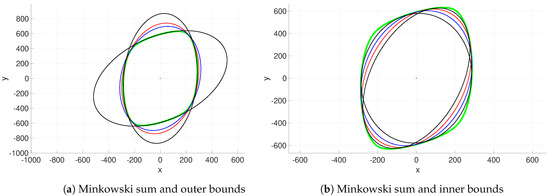
Figure 1.
Green: Minkowski sum, red: Kurzhanski’s outer for in subplot (a) and Kurzhanski’s inner for in subplot (b), blue: MVOE in subplot (a) and John’s inner in subplot (b) and black: Kurzhanski’s outer for in subplot (a) and also Kurzhanski’s inner for two arbitrary nonidentity matrices of in subplot (b).
Aside from the ellipsoidal bounds reviewed above, ellipsoidal approximations of the Minkowski sum are also developed here, which in contrast to the bounds, they neither necessarily enclose the Minkowski sum from outside nor are they fully contained inside the Minkowski sum. However, they are used later, as well as the inner and outer bounds, to derive a closed-form model of the slice of Minkowski sum. These ellipsoidal approximations are constructed from replacing the parametrized positive scalar term for in the denominator of the Minkowski Formula (4) with some fixed positive scalars . As discussed above, this is due to the fact that the sum of finite numbers of symmetric positive definite matrices , for any positive constant , is a symmetric positive definite matrix, which parametrizes an ellipsoidal approximation of the corresponding Minkowski sum in (4). Here, in , each denominator in the Minkowski sum (4) is replaced by the second eigenvalue of the matrix or by the Frobenius norm of the matrix , so that the explicit parametric relation of the family of ellipsoidal approximations of the Minkowski sum is obtained by:
or by:
where each ellipsoidal approximation is centered at , denotes the dimension of the space and is the Frobenius norm of the matrix . In this work, for any , the three positive eigenvalues are assumed to be sorted as .
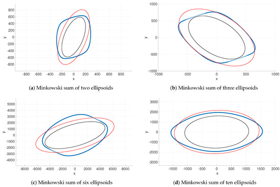
Figure 2 illustrates some ellipsoidal approximations, obtained from (14) and (15), for various geometries of the Minkowski sums of two, three, six and ten numbers of ellipsoids in with different sizes of semi-axes and orientations. As the results show, the ellipsoidal approximations do not necessarily bound the Minkowski sum from outside or inside. It is notable that the ellipsoid obtained from Frobenius norm in (15) shows more level of accuracy relative to the actual Minkowski sum. Although these ellipsoids do not approximate the Minkowski sum precisely, they could be used in derivation of the closed-form explicit parametric equation of the slice of Minkowski sum of ellipsoids, as discussed in the following section.
3. Slice of Minkowski Sum of Ellipsoids
In this section, a closed-form explicit parametric formula is developed to approximate the slice of Minkowski sum of a finite number of ellipsoids, sliced up by an arbitrarily oriented plane in Euclidean space . This formulation is mathematically of immense interest, since the Minkowski sum of ellipsoids is in general a geometry with an irregular shape, which by nature makes its slice ambiguous. In addition to that, although different closed-form equations of Minkowski sum of ellipsoids were previously developed [12,16], to the best of the author’s knowledge, a closed-form parametrization of the slice of Minkowski sum of finite number of ellipsoids has not been addressed yet. The main idea behind this derivation is first to approximate the Minkowski sum by an ellipsoid and then slice it up by that plane. Then, the resultant elliptical intersection is used to define a sector of a unit sphere, which is composed of a spherical cap and a cone formed by the center of that unit sphere and the base of that cap (see Figure 3). The base of this cone is a circle, which is mapped to an approximation of the slice of Minkowski sum by the same transformation (from the parametric equation of Minkowski sum) that maps the unit sphere to the Minkowski sum.
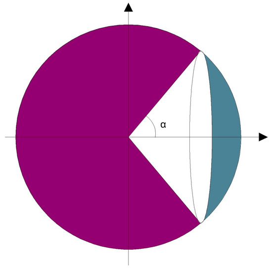
Figure 3.
Sphere and cone with its apex on the center of the sphere.
As discussed in the previous section, there are several ways to bound (see (5), (7), (9), (12)) or approximate (see (14) and (15)) a Minkowski sum of ellipsoids. Consider an ellipsoidal approximation of the boundary of Minkowski sum for , which is centered at and is successively described by the explicit and implicit descriptions and . Note that, here, is a unit vector in that is parametrized by two angles , for instance and , such that it describes the two-dimensional surface of the unit sphere centered at the origin and embedded in . Here, is a symmetric positive definite matrix, which defines the ellipsoidal approximation of the Minkowski sum and could be obtained from either (14) or (15) for as:
where in (16) is the matrix C corresponding to the second eigenvalue .
Let be a generally oriented plane embedded in Euclidean space , that means , where denotes the Euclidean inner product of two vectors, is the normal unit vector of the plane and the so-called “height” of the plane is the component of any arbitrary point on the plane, along the normal unit vector . Now, slice up the ellipsoidal approximation of the Minkowski sum by the plane P, where the elliptical intersection is parametrized by angles as , such that from implicit definition of , . This implies , where the unit vector is defined by . Since both and are unit vectors, hence
is used to define a sector of a unit sphere. This sector is a portion of the unit sphere and is composed of a cone with its apex on the center of the sphere and also of a spherical cap (see Figure 3).
The base of this cone is the circular intersection of the unit sphere centered at the origin and embedded in , which at is sliced up by the plane , defined by the unit normal vector and height , as . Therefore, the circular intersection of the unit sphere with the plane is centered at and has the radius of . Using the unit vector , let us define two other unit vectors and , such that forms an orthonormal basis. Then, this orthonormal basis is used to determine the orientation of the circular intersection by matrix . Therefore, the circular intersection of the unit sphere and the slicing plane is explicitly parametrized by the angle as:
where is a unit vector in that is parametrized by one angle , such that it describes the one-dimensional circumference of the unit circle centered at the origin and embedded in plane . Now, an approximation of the slice of Minkowski sum is suggested by mapping this circular base of the cone in (19) using the same transformation (from the parametric Equation (4) of Minkowski sum), which maps the unit sphere to the Minkowski sum. Therefore, the slice of Minkowski sum of ellipsoids by an arbitrarily oriented plane in is explicitly parametrized as a curve embedded in by:
The planar slice of Minkowski sum is finally obtained from projection of this curve onto the slicing plane P along the normal unit vector of the plane. This means that the planar slice of Minkowski sum is explicitly parametrized by:
where for any arbitrary point on the slicing plane. It is notable that the necessary and sufficient condition under which the arbitrarily oriented plane P slices up the ellipsoidal approximation of the Minkowski sum is:
which is consistent with (18).
Figure 4 shows a sample of one Minkowski sum of two ellipsoids, sliced up by an arbitrarily oriented plane at different heights of h, for which the actual slice is modeled by the parametric formula in (20) (and its projection onto the slicing plane in (21)), based on three various ellipsoidal approximations of Minkowski sum. Recall that the formulation of parametric Equation (20) of the slice of Minkowski sum is based on calculating the circular base (19) of a cone, for which an ellipsoidal approximation of the Minkowski sum is required. Among various ellipsoidal outer and inner bounds and also ellipsoidal approximations of the Minkowski sum introduced above, the MVOE from the minimization of (7), John’s maximum volume inner bound (12) and the ellipsoidal approximation by matrix in (16) from the second eigenvalue for are selected here for computing the parametric slice of Minkowski sum (20). In fact, the MVOE and John’s maximum volume inner ellipsoid are selected successively as the optimal representatives of the family of parametrized outer Kurzhanski’s (7) and inner Kurzhanski’s (9) bounds. Recall that, here, three positive eigenvalues of any symmetric positive definite matrix are assumed to be sorted in ascending order; therefore, the ellipsoidal approximation of the Minkowski sum by second eigenvalue is assumed to be a moderate approximation, wisely chosen for computation of a parametric slice of Minkowski sum. The Minkowski sum in this sample is constructed from two ellipsoids with an aspect ratio of 3, which is the ratio of the length of the major axis (longest axis) to the length of the minor axis (shortest axis).
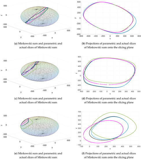
Figure 4.
Parametric slices of Minkowski sum for a particular Minkowski sum and orientation of the slicing plane but at different heights h, computed by: MVOE from minimization of (7) (black), John’s inner bound in (12) (blue), second eigenvalue in (16) (green). The actual slice of Minkowski sum is pink.
Figure 4 illustrates both the parametric slices of Minkowski sum embedded in and the corresponding projections onto the slicing plane. Figure 4a,b corresponds to the case in which the slicing plane is close to the center of the Minkowski sum, such that the curve of the actual slice is relatively far enough from the zones of the Minkowski surface with high curvature, namely the “corners” of the Minkowski surface. In such cases, the suggested technique above for modeling the actual slice by (20) and (21) generally provides reliable approximation of the actual slice, such that the accuracy and consistency of the parametric slice with the actual one increase when the actual slice is farther from the “corners” of the Minkowski surface. Precisely, the parametric slice, computed by matrix in (16) from the second eigenvalue for presents a more consistent approximation with the actual slice of Minkowski sum. In other words, the second eigenvalue-based parametric formula of the slice of Minkowski sum models the actual slice more accurately compared with the Kurzhanski’s outer–inner bound-based parametric formulas of the slice. Here, the matrix of normalized error is calculated, for verification purpose, to measure the accuracy of the developed parametric slice of Minkowski sum, as:
where again denotes the Frobenius matrix norm, is a matrix for denoting the number of points on either parametric or actual slice, and, also, and , respectively, denote the matrices that form the points of the parametric slice and actual slice of the Minkowski sum as the rows in descending order. Note that denotes the set of positive integer numbers. This error is in the form of distances between points from the parametric slice and actual slice, normalized by the Frobenius norm. The calculation of the normalized error matrix for parametric slice, computed by matrix in (16) from the second eigenvalue for , shows that the normalized distance between a point of parametric slice and a point of actual slice is less than , that is, for each row . In other words, the normalized error is less than for the parametric slice, computed by matrix in (16) from the second eigenvalue for . Figure 4c–f illustrates identical samples of Minkowski sum to Figure 4a,b, sliced up by the same oriented plane, but at larger heights of h, for which the parametric slices present weaker approximations. This observation approves the hypothesis that by increasing the distance of the slicing plane from the center of the Minkowski sum toward the “corners”, the parametric model will lose accuracy.
Figure 5 enlightens that the weak consistency of the slice approximations with the actual one, observed in Figure 4c–f, is in fact an indirect consequence of the distance of the slicing plane (actual slice) from the center of the Minkowski sum. This figure shows a similar slicing sample to Figure 4a,b, such that the same Minkowski sum is sliced up by a plane at the same height h but with different orientation. Although, the slicing plane is in the same distance h from the Minkowski center, as in Figure 4a,b, the parametric slices show some discrepancy with the actual one at two corners of the projected (planar) slices (see Figure 5b). These corners of the planar slices correspond to the slicing of the corners of the Minkowski sum with high curvatures (see Figure 5a). In summary, the comparison between Figure 4a,b and Figure 5a,b implies that the inconsistency between the parametric slice and actual slice of Minkowski sum occurs in the case that the curve of the actual slice passes closely through the corners of the Minkowski surface with high curvature, where the parametric model presents lower accuracy of approximation.
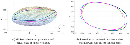
Figure 5.
Parametric slices of Minkowski sum for similar Minkowski sum and height h of slicing plane to the sample in Figure 4a,b but for a different orientation of the plane. The parametric slices are computed by: MVOE from minimization of (7) (black), John’s inner bound (12) (blue) and the second eigenvalue in (16) (green). The actual slice of Minkowski sum is pink.
In line with the current discussion of the destructive impact of curvature of the Minkowski surface on the accuracy of the suggested parametric model for the slice of Minkowski sum, Figure 6 represents another type of condition under which the Minkowski surface might likely have high curvature at particular zones. This is the case in which the constituting ellipsoids of the Minkowski sum have a “strong” high aspect ratio. For an ellipsoid with a “strong” high aspect ratio, not only the ratio of the lengths of major semi-axis (third semi-axis) to the minor semi-axis (first semi-axis) is high but also this ratio is high between the major semi-axis and the second semi-axis, so that the ellipsoid has a “cigar” shape. For the same reason as the high curvature of the Minkowski surface, the parametric approximation of the slice of Minkowski sum of two cigar ellipsoids shows weak modeling of the actual slice.
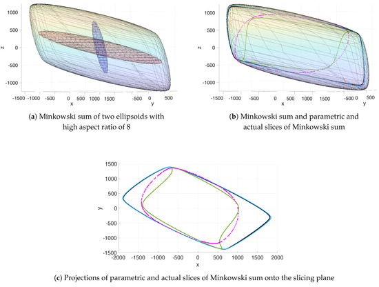
Figure 6.
Parametric slices of Minkowski sum for a Minkowski sum of two ellipsoids with high aspect ratio of 8, sliced up by a similar plane to the sample in Figure 4a,b. The parametric slices are computed by: MVOE from minimization of (7) (black), John’s inner bound (12) (blue) and the second eigenvalue in (16) (green). The actual slice of Minkowski sum is pink.
4. Alternative Algorithm of a Narrow Strip for a Slice of Minkowski Sum
In this section, a computational algorithm is introduced to determine a “narrow strip” around the slice of Minkowski sum of ellipsoids, as an alternative approximation in the cases that the suggested parametric model of the slice returns a weak approximation. As discussed above, in regard to Figure 4e,f, Figure 5 and Figure 6, these failure cases basically correspond to the slicing conditions in which the curve of the actual slice is closely passing through “corners” of the Minkowski surface with high curvatures.
Here, the algorithm is demonstrated for the slice of Minkowski sum of two ellipsoids in . This strategy was basically inspired by the rationale behind (10) and (11), which indicates that the Minkowski sum of two ellipsoids, , could be precisely constructed from the intersection of a countably infinite number of outer bounds from (7) or, similarly, from the union of a countably infinite number of inner bounds from (9). The idea is to determine a “narrow strip” around the slice of Minkowski sum by using a few numbers of outer and inner ellipsoidal bounds of the Minkowski sum. In other words, it is expected that the elliptical slices of a few outer and inner ellipsoidal bounds of the Minkowski surface could be used to form a narrow strip around the slice of that Minkowski surface. Consider the Minkowski sum of two ellipsoids which is sliced up far from the center of that Minkowski sum and close to its corner, as displayed in Figure 7a. A number of outer and inner bounds of the Minkowski are chosen and sliced up by the plane. In this example, the elliptical slices of three ellipsoidal outer bounds are used to form an outer bound of the slice of Minkowski sum, namely the slices of the MVOE from minimization of (7) and two outer Kurzhanski’s bounds from (7) for and , as shown in Figure 7a.b. It is predictable from Figure 1 that, in general, Kurzhanski’s outers for and touch a wider region of the boundary of Minkowski sum. Similarly, Figure 7a,c shows elliptical slices of three ellipsoidal inner bounds, namely the slices of John’s inner bound from (12) and two Kurzhanski’s inner bounds from (9) for two , which are used to form the inner bound of the slice of Minkowski sum. It is notable from Figure 7b,c that the slices of MVOE and John’s bound are not necessarily the minimum area outer ellipse and the maximum area inner ellipse, respectively, among the elliptical slices of all the outer and inner Kurzhanski’s bounds. This is due to the fact that the size of the elliptical slices of the ellipsoidal bounds of the Minkowski sum depends not only on the size of the bounds but also on the orientation of the slicing plane. Then, an arbitrary point, called the “new reference”, is picked inside the slice of one of the inner bounds of the Minkowski sum. This new reference point is surely located inside the actual slice of Minkowski sum, since it is already inside the slice of one inner bound. The new reference point is shown in blue color in Figure 7 for differentiation from the original reference point in red. This new reference point inside the actual slice is then used to find the one closest point to the actual slice (means also closest to the new reference point) among the three existing points on the three slices of outer bounds at every radial position within , measured from the new reference point. Similarly, by applying this technique to three slices of three inner bounds, the set of closest inner points to the actual slice (means farthest to the new reference point) is determined. As a result, the loci of the closest points of the slices of outer and inner bounds to the actual slice form an outer bound (blue curve) and an inner bound (green curve) of the actual slice, which encloses it within a narrow strip as shown in Figure 7d. This algorithm is discussed in more details through several Algorithms A1–A11 in Appendix A.

Figure 7.
(a) Minkowski sum and six slices of Minkowski sum by three outer and three inner bounds of the Minkowski sum and also the actual slice of Minkowski sum, embedded in . (b) Projections of three slices of three outer bounds onto the slicing plane and also the actual slice of Minkowski sum, where slice 1 corresponds to MVOE, slice 2 corresponds to outer Kurzhanski’s with and slice 3 corresponds to outer Kurzhanski’s with . (c) Projections of three slices of three inner bounds onto the slicing plane and also the actual slice of Minkowski sum, where slice 1 corresponds to John’s inner bound, and slices 2 and 3 correspond to inner Kurzhanski’s with two arbitrary . (d) Strip for an actual slice of Minkowski sum (pink dotted curve) obtained from the computational algorithm, using the slices of outer and inner bounds in (b,c). Note that in subplots (b), (c,d), the single red point indicates the origin of the coordinate system and the single blue point is an arbitrary point inside the actual slice.
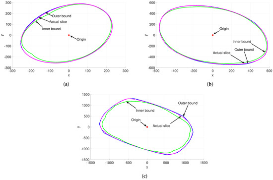
This algorithm might be implemented for more numbers of outer and inner bounds of the Minkowski sum to increase the consistencies of the generated outer and inner bounds of the actual slice to the actual slice, and consequently narrow the strip. For instance, more numbers of outer bounds could be used from the family of Kurzhanski’s outers in (7), parametrized by and, similarly, more numbers of inner bounds from the family of inner Kurzhanski’s in (9) for . Figure 8a represents a narrower strip for the same actual slice in Figure 7, obtained by using MVOE, four outer Kurzhanski’s, John’s inner and four inner Kurzhanski’s bounds. Figure 8b,c approximates the same actual slice by successively using MVOE and eight outer Kurzhanski’s, and then MVOE and ten outer Kurzhanski’s, as both approximations precisely coincide on the actual slice. In other words, the results in Figure 8b,c confirm that the suggested computational algorithm generates a strip that can narrow persistently for a few more numbers of constructing bounds to precisely coincide on the actual slice of Minkowski sum. It means that the possible error of the suggested computational algorithm in the form of discrepancy between the actual and parametric slices is negligible for a small number of constructing bounds. Note that these precise approximations are only constructed from more numbers of Kurzhanski’s outers, since as observed from the comparison between Figure 1a,b, it is predictable that in general an outer ellipsoidal bound touches a wider region of the boundary of Minkowski sum, compared with the touching region between an inner ellipsoid and the Minkowski sum boundary.
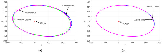
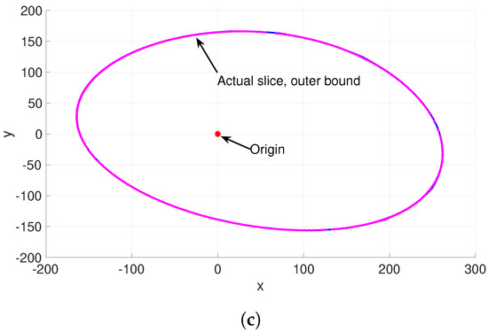
Figure 8.
Strips for a similar actual slice of Minkowski sum (pink) with Figure 7, generated by (a): MVOE, four outer Kurzhanski’s, John’s inner and four inner Kurzhanski’s, (b): MVOE and eight outer Kurzhanski’s, (c): MVOE and ten outer Kurzhanski’s.
5. Discussion
In this work, a closed-form parametric equation was formulated, for the first time, to approximate the slice of Minkowski sum of finite number of ellipsoids in the case that the actual slice is relatively far enough from the corners of the Minkowski sum with high curvatures. In this case, the results show that the normalized error, in the form of normalized distances between points from parametric slice and actual slice, is less than for the parametric slice, computed by matrix from the second eigenvalue for . Alternatively, an algorithm was suggested in the case that the actual slice passes closely through the corners of the Minkowski surface, in which a family of ellipsoidal inner and outer bounds of the Minkowski sum was used to construct a “narrow strip” for the slice of Minkowski sum. The algorithm was also applied in the case of slicing the Minkowski surface of ellipsoids with high aspect ratio. The results approve that more numbers of outer and inner bounds of the Minkowski sum would increase the accuracies of the generated outer and inner bounds of the actual slice, and consequently narrow the enclosing strip of the actual slice. In other words, the results confirm that the suggested computational algorithm generates a strip that can narrow persistently for a few more numbers of constructing bounds to precisely coincide on the actual slice of Minkowski sum. It means that the possible error of the suggested computational algorithm in the form of discrepancy between the actual and parametric slices is negligible for a small number of constructing bounds. In line with the goal, some ellipsoidal inner and outer bounds of the Minkowski sum were reviewed, including Kurzhanski’s bounds. Furthermore, some ellipsoidal approximations of the Minkowski sum were suggested, which do not necessarily bound the Minkowski sum from outside or inside; however, they can be used, as well as the inner and outer bounds, in calculation of the developed parametric approximation of the slice of Minkowski sum. Precisely, the second eigenvalue-based parametric formula presented a more consistent approximation with the actual slice of Minkowski sum, compared with the outer–inner bound-based parametric formulas of the slice.
Funding
This research received no external funding.
Data Availability Statement
The research data is accessible by direct contact to the author.
Acknowledgments
This topic was suggested to the author by Gregory S. Chirikjian, and is greatly appreciated.
Conflicts of Interest
The author declares no conflict of interest.
Appendix A. Algorithms
| Algorithm A1 Function: Slicing plane |
|
| Algorithm A2 Function: Domain of Kurzhanski’s outer bounds |
|
| Algorithm A3 Function: Compute a Kurzhanski’s outer bound |
|
| Algorithm A4 Function: Compute a Kurzhanski’s inner bound |
|
| Algorithm A5 Function: Compute MVOE [29] |
|
| Algorithm A6 Function: Compute the John’s inner bound |
|
| Algorithm A7 Function: Calculate elliptical slice of an ellipsoidal bound |
|
| Algorithm A8 Function: Choose a new origin inside the actual slide of Minkowski sum |
|
| Algorithm A9 Function: Switch the origin to the new one |
|
| Algorithm A10 Function: Outer layer of a strip of the slice of Minkowski sum |
|
| Algorithm A11 Function: Inner layer of a strip of the slice of Minkowski sum |
|
References
- Ruan, S.; Poblete, K.L.; Wu, H.; Ma, Q.; Chirikjian, G.S. Efficient Path Planning in Narrow Passages for Robots With Ellipsoidal Components. IEEE Trans. Robot. 2022. [Google Scholar] [CrossRef]
- Latombe, J.C. Robot Motion Planning, 1st ed.; Springer US: Berlin/Heidelberg, Germany, 1991. [Google Scholar]
- Hartquist, E.E.; Menon, J.P.; Suresh, K.; Voelcker, H.B.; Zagajac, J. A computing strategy for applications involving offsets, sweeps, and Minkowski operations. Comput. Aided Des. 1999, 31, 175–183. [Google Scholar] [CrossRef]
- Halperin, D.; Latombe, J.C.; Wilson, R.H. A General Framework for Assembly Planning: The Motion Space Approach. Algorithmica 2000, 26, 577–601. [Google Scholar] [CrossRef]
- Shiffman, B.; Lyu, S.; Chirikjian, G.S. Mathematical aspects of molecular replacement. V. Isolating feasible regions in motion spaces. Acta Crystallogr. Sect. A 2020, 76, 145–162. [Google Scholar] [CrossRef] [PubMed]
- Chirikjian, G.S.; Shiffman, B. Collision-free configuration-spaces in macromolecular crystals. Robotica 2016, 34, 1679–1704. [Google Scholar] [CrossRef][Green Version]
- Rossmann, M.G.; Blow, D.M. The detection of sub-units within the crystallographic asymmetric unit. Acta Crystallogr. 1962, 15, 24–31. [Google Scholar] [CrossRef]
- Chirikjian, G.S. Mathematical aspects of molecular replacement. I. Algebraic properties of motion spaces. Acta Crystallogr. Sect. A 2011, 67, 435–446. [Google Scholar] [CrossRef]
- Chirikjian, G.S.; Yan, Y. Mathematical aspects of molecular replacement. II. Geometry of motion spaces. Acta Crystallogr. Sect. A 2012, 68, 208–221. [Google Scholar] [CrossRef]
- Chirikjian, G.S.; Sajjadi, S.H.; Toptygin, D.A.; Yan, Y. Mathematical aspects of molecular replacement. III. Properties of space groups preferred by proteins in the Protein Data Bank. Acta Crystallogr. Sect. A Found. Adv. 2015, 71 Pt 2, 186-94. [Google Scholar] [CrossRef]
- Chirikjian, G.S.; Sajjadi, S.; Shiffman, B.; Zucker, S.M. Mathematical aspects of molecular replacement. IV. Measure-theoretic decompositions of motion spaces. Acta Crystallogr. Sect. A 2017, 73, 387–402. [Google Scholar] [CrossRef]
- Yan, Y.; Chirikjian, G.S. Closed-form characterization of the Minkowski sum and difference of two ellipsoids. Geom. Dedicata 2015, 177, 103–128. [Google Scholar] [CrossRef]
- Chirikjian, G.S. Harmonic Analysis for Engineers and Applied Scientists: Updated and Expanded Edition; Dover: New York, NY, USA, 2016. [Google Scholar]
- Dummit, D.S.; Foote, R.M. Abstract Algebra, 3rd ed.; Wiley: New York, NY, USA, 2003. [Google Scholar]
- Hungerford, T.W. Algebra, 8th ed.; Springer: Berlin/Heidelberg, Germany, 1980. [Google Scholar]
- Chirikjian, G.S.; Shiffman, B. Applications of convex geometry to Minkowski sums of m ellipsoids in Rn: Closed-form parametric equations and volume bounds. Int. J. Math. 2021, 32, 2140009. [Google Scholar] [CrossRef]
- Ruan, S.; Chirikjian, G.S. Closed-form Minkowski sums of convex bodies with smooth positively curved boundaries. Comput.-Aided Des. 2022, 143, 103133. [Google Scholar] [CrossRef]
- Alfano, S.; Greer, M.L. Determining If Two Solid Ellipsoids Intersect. J. Guid. Control Dyn. 2003, 26, 206–210. [Google Scholar] [CrossRef]
- Goodey, P.; Weil, W. Intersection bodies and ellipsoids. Mathematika 1995, 42, 295–304. [Google Scholar] [CrossRef]
- Perram, J.W.; Wertheim, M.S. Statistical mechanics of hard ellipsoids. I. Overlap algorithm and the contact function. J. Comput. Phys. 1985, 58, 409–416. [Google Scholar] [CrossRef]
- Kurzhanski, A.; Valyi, I. Ellipsoidal Calculus for Estimation and Control, 1st ed.; Systems and Control: Foundations and Applications; Birkhäuser Basel: Basel, Switzerland, 1997. [Google Scholar]
- Kurzhanskiy, A.A.; Varaiya, P. Ellipsoidal Toolbox (ET). In Proceedings of the 45th IEEE Conference on Decision and Control, San Diego, CA, USA, 13–15 December 2006; pp. 1498–1503. [Google Scholar]
- Ros, L.; Sabater, A.; Thomas, F. An ellipsoidal calculus based on propagation and fusion. IEEE Trans. Syst. Man Cybern. Part B (Cybern.) 2002, 32, 430–442. [Google Scholar] [CrossRef]
- Durieu, C.; Walter, É.; Polyak, B.T. Multi-Input Multi-Output Ellipsoidal State Bounding. J. Optim. Theory Appl. 2001, 111, 273–303. [Google Scholar] [CrossRef]
- Sholokhov, O.V. Minimum-volume ellipsoidal approximation of the sum of two ellipsoids. Cybern. Syst. Anal. 2011, 47, 954–960. [Google Scholar] [CrossRef]
- Kurzhanski, A.; Varaiya, P. Reachability analysis for uncertain systems-The ellipsoidal technique. Dyn. Contin. Discret. Impuls. Syst. Ser. B Appl. Algorithms 2002, 9, 347–368. [Google Scholar]
- Schweppe, F. Uncertain Dynamic Systems; Prentice-Hall: Englewood Cliffs, NJ, USA, 1973. [Google Scholar]
- Maksarov, D.; Norton, J.P. State bounding with ellipsoidal set description of the uncertainty. Int. J. Control 1996, 65, 847–866. [Google Scholar] [CrossRef]
- Halder, A. On the Parameterized Computation of Minimum Volume Outer Ellipsoid of Minkowski Sum of Ellipsoids. In Proceedings of the 2018 IEEE Conference on Decision and Control (CDC), Miami Beach, FL, USA, 17–19 December 2018; Volume 1, pp. 4040–4045. [Google Scholar]
- Busemann, H. The foundations of Minkowskian geometry. Comment. Math. Helv. Vol. 1950, 24, 156–187. [Google Scholar] [CrossRef]
- John, F. Extremum Problems with Inequalities as Subsidiary Conditions. In Traces and Emergence of Nonlinear Programming; Birkhäuser Basel: Basel, Switzerland, 2014; pp. 197–215. [Google Scholar]
- Chernousko, F.L. State Estimation for Dynamic Systems, 1st ed.; CRC Press: Boca Raton, FL, USA, 1993. [Google Scholar]


Disclaimer/Publisher’s Note: The statements, opinions and data contained in all publications are solely those of the individual author(s) and contributor(s) and not of MDPI and/or the editor(s). MDPI and/or the editor(s) disclaim responsibility for any injury to people or property resulting from any ideas, methods, instructions or products referred to in the content. |
© 2022 by the author. Licensee MDPI, Basel, Switzerland. This article is an open access article distributed under the terms and conditions of the Creative Commons Attribution (CC BY) license (https://creativecommons.org/licenses/by/4.0/).