Assessment of Structural Systems to Design Earthquake Resistance Buildings by Employing Multi-Attribute Decision-Making Method Based on the Bipolar Complex Fuzzy Dombi Prioritized Aggregation Operators

Abstract

An earthquake is a natural phenomenon that occurs when two tectonic plates in the earth’s crust move against each other. This movement creates seismic waves that can cause the ground to shake, sometimes resulting in damage to buildings and infrastructure. It is important to be prepared for earthquakes, particularly if you live in an area that is at high risk for seismic activity. This includes having an emergency kit, knowing how to shut off utilities, having a plan in place for what to do in the event of an earthquake, and most importantly, constructing earthquake resistance buildings. The assessment and the ranking of structural systems to design earthquake resistance buildings is a MADM (multi-attribute decision-making) dilemma. Consequently, in this script, we initiate the method of MADM under the bipolar complex fuzzy (BCF) information. For this method, we devise BCF Dombi prioritized averaging (BCFDPA), BCF Dombi prioritized weighted averaging (BCFDPWA), BCF Dombi prioritized geometric (BCFDPG), and BCF Dombi prioritized weighted geometric (BCFDPPWG) operators by utilizing the Dombi aggregation operator (AO) with BCF information. After that, by using artificial data, we assess the structural systems to design earthquake resistance buildings with the assistance of the invented method of MADM. To exhibit the dominancy and supremacy of the elaborated work, the advantages, sensitive examination, graphical representation, and comparative study are described in this script.

1. Introduction

Earthquakes are natural disasters that can cause significant damage to buildings, infrastructure, and human life. Earthquakes are a natural consequence of plate tectonics, which is the movement and interaction of Earth’s crustal plates. Studying earthquakes can provide valuable insights into the structure and behavior of these plates, as well as the dynamics of the earth’s interior. Earthquakes play a crucial role in shaping the earth’s surface. The movement of tectonic plates can create mountain ranges, valleys, and other geologic features. Earthquakes can also trigger landslides and volcanic eruptions, which can have a significant impact on the environment. Earthquakes can also cause structural damage to buildings and infrastructure, including collapses, cracking, and shifting. This can result in property damage and loss of life. Structural systems are essential in designing earthquake-resistant buildings. They provide strength, stability, and resilience to a building, which can minimize or prevent damage during an earthquake. Here are some key reasons why structural systems are important in earthquake-resistant building design:

• Resist lateral forces: Earthquakes generate lateral forces that can cause buildings to sway, twist, or collapse. Structural systems provide resistance against these forces by providing a strong framework and bracing elements that can resist and transfer lateral loads.
• Absorb seismic energy: When an earthquake occurs, it generates seismic waves that can cause buildings to vibrate. Structural systems can be designed to absorb and dissipate this energy through various means, such as damping systems, base isolation, and energy-dissipating devices.
• Support gravity loads: A building’s weight and the weight of its contents can add to the forces acting on it during an earthquake. Structural systems can provide support for the building’s gravity loads, reducing the chance of collapse.
• Maintain stability: Structural systems can help maintain a building’s stability during an earthquake by providing redundancy and ensuring that key load-bearing elements remain intact. This can prevent the building from tipping over or collapsing.
• Facilitate rapid recovery: In the event of an earthquake, a building with a well-designed structural system can be repaired and made operational more quickly than a building with inadequate structural support. This can minimize downtime and help communities recover more rapidly.

Overall, a well-designed structural system is critical for ensuring the safety and resilience of a building during an earthquake. Building codes and standards often require specific structural features and design principles to ensure that structures can withstand seismic forces. Grigorian et al. [1] studied sustainable earthquake-resistant mixed multiple seismic systems. Scalvenzi et al. [2] discussed the progressive collapse fragility of substandard and earthquake-resistant precast RC buildings. A novel seismic resisting system was established by Maroofi et al. [3]. You et al. [4] discussed the effects of self-centering structural systems on resilience. Shi [5] analyzed super high-rise building structure design. Hanafy [6] discussed the fuzzy $\beta$-compactness and $\beta$-closed spaces. Bhavanari and Kuncham [7] invented fuzzy cosets and Yun et al. [8] interpreted fuzzy maximal ideals of $\Gamma$-nearrings. Zhang et al. [9] invented the WEPLPA-CPT-EDAS approach.

In the real world, due to the rising difficulty of the socioeconomic nature and the absence of information or knowledge about the issue domain, crips data are occasionally absent. Consequently, the input values might be ambiguous or hazy in nature. Atanassov [10] presented the conception of an intuitionistic fuzzy set (IFS) which carries a supportive grade (SG) and non-supportive grade (NSG) such that their sum belongs to the closed interval $\left[0, 1\right]$. The IFS is the modification of the FS [11], which merely carries an SG. Liu et al. [12] utilized Dombi operations (DOs) in IFS and created MADM issues utilizing Dombi Bonferroni mean operator. Zeng et al. [13] devised the MCDM technique under IFS. Xu and Yager [14] described a few geometric AO (GAO) based on intuitionistic FS. Zhao et al. [15] presented certain AO in the setting of IFS. A new AO for IFS along with applications was given by Ngyuen [16]. Alcantud et al. [17] interpreted an aggregation of infinite chains of IFS. The induced generalized AO for IFS and their application in group DM were given by Xu and Wang [18]. Yu and Xu [19] presented the prioritized IF AO. Yu [20] defined a multi-criteria DM (MCDM) based on generalized prioritized AO in the setting of IFS. Seikh and Mandal [21] presented IF Dombi AO (DAO). Zeng et al. [22] interpreted distance measure for fermatean FS and Yang et al. [23] devised weighted distance measures for fermatean FS.

From the study of an object, we know that for every property of an object, there is a counter property. To cope with uncertainties and ambiguities in genuine life issues, IFS is indispensable, but can’t handle the counter property of the object. For this, Zhang [24,25] interpreted a new concept, called bipolar FS (BFS). The theory of BFS carries the information of the property and counter property of the object in the structure of positive grade of membership (PGM) and negative grade of membership (NGM), where PGM belongs to $\left\{0, 1\right\}$ and NGM belongs to $\left\{-1, 0\right\}$. The theory of BFS is utilized in numerous disciplines like medical science [26,27], bipolar quantum logic-based computing [28,29], biosystem regulation [30], computational psychiatry [31], and more. Soon after, Gul [32] described bipolar fuzzy (BF) AO. The BF Domi prioritized AO (DPAO) were diagnosed by Jana et al. [33]. The Dombi AO in the setting of BFS was presented by Jana et al. [34]. Gao et al. [35] diagnosed Hamacher-prioritized AO for dual-hesitant BF and utilized them in MADM. Wei et al. [36] interpreted BF Hamacher AO. Abdullah et al. [37] presented bipolar fuzzy SS. Jana et al. [38] described a robust AO for the multi-criteria DM method with BF soft environment. Mustafa [39] devised bipolar soft ideal rough set.

In real-world issues, decision-makers sometimes face problems where vagueness and uncertainty are involved in two dimensions. To handle this problem, Ramot et al. [40] propounded the initial idea of complex FS (CFS) containing a grade of membership (GM) in the polar form containing a unit circle of a complex plane. Afterward, Tamir et al. [41] introduced CFS in the Cartesian form (the MG belongs to the unit square in a complex plane). Zhang et al. [42] organized operation properties in the setting of CFS. Ramot et al. [43] described complex fuzzy (CF) logic. Greenfield [44] investigated the conception of interval-valued CF logic (CFL). Tamir et al. [45] interpreted CF sets and CFL as an overview of theory and applications. Yazdanbakhsh and Dick [46] gave a systematic review of complex FS and logic. The CF arithmetic AO were defined by Bi et al. [47]. Bi et al. [48] introduced CF geometric AO. Dai et al. [49] presented interval-valued CF geometric AO and their application to DM. Hu et al. [50] concocted CF power AO. A decision analyst or expert requires the notion of BFS to express the positive and negative opinions about the objects or elements and requires the notion of CF set to express the two-dimensional information of the object, but when a decision analyst or expert is required to express the positive pole and negative pole (positive and negative opinions) along with two-dimensional then he/she needs a different mathematical structure which was invented by Mahmood and Ur Rehman [51], termed BCFS. In [51], they also investigated various similarity measures (SMs) under BCFS and their applications to medical diagnosis and pattern recognition. Afterward, Mahmood et al. [52] used an approach of MADM relying on the Hamacher-AO under bipolar complex fuzzy (BCF) information. Mahmood and Ur Rehman [53] also invented an approach of MADM relying on Dombi AO for BCF information. Further, for coping with decision-making (DM) dilemmas, Mahmood et al. [54] deduced a DM technique relying on the Aczel-Alsina AO under the model of BCFS. The decision support system under BCF information relying on the AO was developed by Mahmood et al. [55]. A novel DM approach that is an AHP technique for BCFS relying on Frank AO was investigated by Ur Rehman [56].

Aggregation operators (AO), generally carrying the shapes of a mathematical tool, are frequent methods to combine all the information into one. Because of their huge significance in the data management of wide fields, like information retrieval, data mining, pattern recognition, medical diagnosis, machine learning, decision making (DM), the study on AO has been getting a lot of interest from both scholars and experts over recent decades [57,58,59]. The Dombi t-norm and t-conorm were initially initiated by Dombi [60] in 1982. The parameter value makes the Dombi t-norm and t-conorm operators more flexible and beneficial. By varying the parameter values, the resulting norm varies. Further, in genuine MADM dilemmas, for experts or decision analysts, usually the priority level of every attribute is distinct. Thus, there is always the requirement for the priority AO for the method of MADM. Keep in mind that the BCFS is a perfect tool and model for tackling the awkward and tricky information in genuine-life dilemmas and the need for the priority AO; the benefits of the Dombi operators provide us with the necessary encouragement to compose this article. The Dombi prioritized AO are not yet expanded to aggregate BCF information. In this manuscript, we expand the Dombi prioritized AO in the model of BCFS to investigate BCFDPA, BCFDPWA, BCFDPG, and BCFDPWG operators. Moreover, we elaborate a method of MADM based on the invented AO and assess the structural systems to design earthquake resistance buildings.

The remaining article is formalized as follows:

• In Section 2, we review basic notions, such as BCFS, its elementary operations, Dombi operations, and the definition of prioritized AO.
• In Section 3, we devise Dombi-prioritized arithmetic aggregation (DPAA) operators and Dombi-prioritized geometric aggregation (DPGA) operators in the environment of BCF information. These AO are BCFDPA, BCFDPWA, BCFDPG, and BCFDPWG operators.
• In Section 4, of this study, we create the MADM method employing the BCF Dombi prioritized aggregation (BCFDPA) operators that is BCFDPWA and BCFDPWG operators, and then develop a real-life MADM problem to describe the application of deciphered operators. Further, we investigated the impact of the parameter on MADM outcomes in Section 4.
• In Section 5, a comparison of the diagnosed work with prevailing works is given, to expose the importance and supremacy of the proposed work.
• The concluding remarks of this research manuscript are presented in Section 6.

2. Basic Concepts and Operations

In this Section, we present basic notions of BCFS, their elementary operational laws, Dombi operations, and the definition of prioritized AO. In this article, $\stackrel{°}{\mathrm{A}}$ will signify the set of the universe.

2.1. Bipolar Complex Fuzzy Set

Here, we review the concept of the BCF set and its elementary operational laws.

Definition 1

([51]). A set of the model is as follows:

$$\check{\mathrm{R}}=\left\{\left(\stackrel{°}{\mathrm{a}}, {\Gamma }_{\check{\mathrm{R}}}^{+}\left(\stackrel{°}{\mathrm{a}}\right), {\Gamma }_{\check{\mathrm{R}}}^{-}\left(\stackrel{°}{\mathrm{a}}\right)\right) | \stackrel{°}{\mathrm{a}}\in \stackrel{°}{\mathrm{A}}\right\}$$

(1)

is said to be BCF set where ${\Gamma }_{\check{\mathrm{R}}}^{+}\left(\stackrel{°}{\mathrm{a}}\right)={\omega }_{\check{\mathrm{R}}}^{-}\left(\stackrel{°}{\mathrm{a}}\right)+\mathfrak{i} {\varpi }_{\check{\mathrm{R}}}^{-}\left(\stackrel{°}{\mathrm{a}}\right)$ means the positive SG (PSG) and  ${\Gamma }_{\check{\mathrm{R}}}^{-}\left(\stackrel{°}{\mathrm{a}}\right)={\omega }_{\check{\mathrm{R}}}^{-}\left(\stackrel{°}{\mathrm{a}}\right)+\mathfrak{i} {\varpi }_{\check{\mathrm{R}}}^{-}\left(\stackrel{°}{\mathrm{a}}\right)$ means the negative SG (NSG) and ${\omega }_{\check{\mathrm{R}}}^{+}\left(\stackrel{°}{\mathrm{a}}\right),{\varpi }_{\check{\mathrm{R}}}^{+}\left(\stackrel{°}{\mathrm{a}}\right)\in \left[0, 1\right]$ and ${\omega }_{\check{\mathrm{R}}}^{-}\left(\stackrel{°}{\mathrm{a}}\right),{\varpi }_{\check{\mathrm{R}}}^{-}\left(\stackrel{°}{\mathrm{a}}\right)\in \left[-1, 0\right]$. The bipolar complex fuzzy number (BCFN) is distinguished by $\check{\mathrm{R}}=\left({\Gamma }_{\check{\mathrm{R}}}^{+}, {\Gamma }_{\check{\mathrm{R}}}^{-}\right)=\left({\omega }_{\check{\mathrm{R}}}^{+}+\mathfrak{i} {\varpi }_{\check{\mathrm{R}}}^{+}, {\omega }_{\check{\mathrm{R}}}^{-}+\mathfrak{i}{\varpi }_{\check{\mathrm{R}}}^{-}\right).$

Definition 2

([53]). The score value (SV)  ${\mathfrak{J}}_B$  of a BCFN $\check{\mathrm{R}}=\left(\stackrel{°}{\mathrm{a}}, {\Gamma }_{\check{\mathrm{R}}}^{+}\left(\stackrel{°}{\mathrm{a}}\right), {\Gamma }_{\check{\mathrm{R}}}^{-}\left(\stackrel{°}{\mathrm{a}}\right)\right)=\left(\stackrel{°}{\mathrm{a}}, {\omega }_{\check{\mathrm{R}}}^{+}\left(\stackrel{°}{\mathrm{a}}\right)+\mathfrak{i} {\varpi }_{\check{\mathrm{R}}}^{+}\left(\stackrel{°}{\mathrm{a}}\right), {\omega }_{\check{\mathrm{R}}}^{-}\left(\stackrel{°}{\mathrm{a}}\right)+\mathfrak{i}{\varpi }_{\check{\mathrm{R}}}^{-}\left(\stackrel{°}{\mathrm{a}}\right)\right)$ is demonstrated as

$${\mathfrak{J}}_B\left(\check{\mathrm{R}}\right)=\frac{1}{4}\left(2+{\omega }_{\check{\mathrm{R}}}^{+}\left(\stackrel{°}{\mathrm{a}}\right)+{\varpi }_{\check{\mathrm{R}}}^{+}\left(\stackrel{°}{\mathrm{a}}\right)+{\omega }_{\check{\mathrm{R}}}^{-}\left(\stackrel{°}{\mathrm{a}}\right)+{\varpi }_{\check{\mathrm{R}}}^{-}\left(\stackrel{°}{\mathrm{a}}\right)\right), {\mathfrak{J}}_B\in \left[0, 1\right]$$

(2)

Definition 3

([53]). The accuracy funcion ${\mathfrak{A}}_B$ of a BCFN $\check{\mathrm{R}}=\left(\stackrel{°}{\mathrm{a}}, {\Gamma }_{\check{\mathrm{R}}}^{+}\left(\stackrel{°}{\mathrm{a}}\right), {\Gamma }_{\check{\mathrm{R}}}^{-}\left(\stackrel{°}{\mathrm{a}}\right)\right)=\left(\stackrel{°}{\mathrm{a}}, {\omega }_{\check{\mathrm{R}}}^{+}\left(\stackrel{°}{\mathrm{a}}\right)+\mathfrak{i} {\varpi }_{\check{\mathrm{R}}}^{+}\left(\stackrel{°}{\mathrm{a}}\right), {\omega }_{\check{\mathrm{R}}}^{-}\left(\stackrel{°}{\mathrm{a}}\right)+\mathfrak{i} {\varpi }_{\check{\mathrm{R}}}^{-}\left(\stackrel{°}{\mathrm{a}}\right)\right)$ is demonstrated as

$${\mathfrak{A}}_B\left(\check{\mathrm{R}}\right)=\frac{{\omega }_{\check{\mathrm{R}}}^{+}\left(\stackrel{°}{\mathrm{a}}\right)+{\varpi }_{\check{\mathrm{R}}}^{+}\left(\stackrel{°}{\mathrm{a}}\right)-{\omega }_{\check{\mathrm{R}}}^{-}\left(\stackrel{°}{\mathrm{a}}\right)-{\varpi }_{\check{\mathrm{R}}}^{-}\left(\stackrel{°}{\mathrm{a}}\right)}{4}, {\mathfrak{A}}_B\in \left[0, 1\right]$$

(3)

Definition 4

([53]). Suppose that $\check{\mathrm{R}}=\left( {\Gamma }_{\check{\mathrm{R}}}^{+}, {\Gamma }_{\check{\mathrm{R}}}^{-}\right)$ and $\hat{\mathrm{S}}=\left( {\Gamma }_{\hat{\mathrm{S}}}^{+}, {\Gamma }_{\hat{\mathrm{S}}}^{-}\right)$ are two BCFNs, then we have

• If ${\mathfrak{J}}_B\left(\check{\mathrm{R}}\right)<{\mathfrak{J}}_B\left(\hat{\mathrm{S}}\right)$, then $\check{\mathrm{R}}<\hat{\mathrm{S}}$
• If ${\mathfrak{J}}_B\left(\check{\mathrm{R}}\right)>{\mathfrak{J}}_B\left(\hat{\mathrm{S}}\right)$, then $\check{\mathrm{R}}>\hat{\mathrm{S}}$
• If ${\mathfrak{J}}_B\left(\check{\mathrm{R}}\right)={\mathfrak{J}}_B\left(\hat{\mathrm{S}}\right)$, then

i. 

If ${\mathfrak{A}}_B\left(\check{\mathrm{R}}\right)<{\mathfrak{A}}_B\left(\hat{\mathrm{S}}\right),$ then $\check{\mathrm{R}}<\hat{\mathrm{S}}$

ii. 

If ${\mathfrak{A}}_B\left(\check{\mathrm{R}}\right)>{\mathfrak{A}}_B\left(\hat{\mathrm{S}}\right),$ then $\check{\mathrm{R}}>\hat{\mathrm{S}}$

iii. 

If ${\mathfrak{A}}_B\left(\check{\mathrm{R}}\right)={\mathfrak{A}}_B\left(\hat{\mathrm{S}}\right),$ then $\check{\mathrm{R}}=\hat{\mathrm{S}}$

Definition 5

([53]). Let $\check{\mathrm{R}}=\left({\Gamma }_{\check{\mathrm{R}}}^{+}, {\Gamma }_{\check{\mathrm{R}}}^{-}\right)=\left({\omega }_{\check{\mathrm{R}}}^{+}+\mathfrak{i} {\varpi }_{\check{\mathrm{R}}}^{+}, {\omega }_{\check{\mathrm{R}}}^{-}+\mathfrak{i} {\varpi }_{\check{\mathrm{R}}}^{-}\right)$ and $\hat{\mathrm{S}}=\left( {\Gamma }_{\hat{\mathrm{S}}}^{+}, {\Gamma }_{\hat{\mathrm{S}}}^{-}\right)=\left({\omega }_{\hat{\mathrm{S}}}^{+}+\mathfrak{i} {\varpi }_{\hat{\mathrm{S}}}^{+}, {\omega }_{\hat{\mathrm{S}}}^{-}+\mathfrak{i} {\varpi }_{\hat{\mathrm{S}}}^{-}\right)$ be two BCFNs, and let $\lambda >0$. Then

• $\check{\mathrm{R}}\oplus \hat{\mathrm{S}}=\left(\begin{array}{c}{\omega }_{\check{\mathrm{R}}}^{+}+{\omega }_{\hat{\mathrm{S}}}^{+}-{\omega }_{\check{\mathrm{R}}}^{+}{\omega }_{\hat{\mathrm{S}}}^{+}+𝔦 {\varpi }_{\check{\mathrm{R}}}^{+}+{\varpi }_{\hat{\mathrm{S}}}^{+}-{\varpi }_{\check{\mathrm{R}}}^{+} {\varpi }_{\hat{\mathrm{S}}}^{+}, \\ -\left({\omega }_{\check{\mathrm{R}}}^{-}{\omega }_{\hat{\mathrm{S}}}^{-}\right)+𝔦 \left(-\left({\varpi }_{\check{\mathrm{R}}}^{-}{\varpi }_{\hat{\mathrm{S}}}^{-}\right)\right)\end{array}\right)$;
• $\check{\mathrm{R}}\otimes \hat{\mathrm{S}}=\left(\begin{array}{c}{\omega }_{\check{\mathrm{R}}}^{+}{\omega }_{\hat{\mathrm{S}}}^{+}+𝔦 {\varpi }_{\check{\mathrm{R}}}^{+} {\varpi }_{\hat{\mathrm{S}}}^{+}, \\ {\omega }_{\check{\mathrm{R}}}^{-}+{\omega }_{\hat{\mathrm{S}}}^{-}+{\omega }_{\check{\mathrm{R}}}^{-}{\omega }_{\hat{\mathrm{S}}}^{-}+𝔦 {\varpi }_{\check{\mathrm{R}}}^{-}+{\varpi }_{\hat{\mathrm{S}}}^{-}+{\varpi }_{\check{\mathrm{R}}}^{-}{\varpi }_{\hat{\mathrm{S}}}^{-}\end{array}\right)$;
• $\lambda \check{\mathrm{R}}=\left(1-{\left(1-{\omega }_{\check{\mathrm{R}}}^{+}\right)}^{\lambda }+\mathfrak{i} \left(1-{\left(1-{\varpi }_{\check{\mathrm{R}}}^{+}\right)}^{\lambda }\right),-{\left|{\omega }_{\check{\mathrm{R}}}^{-}\right|}^{\lambda }+\mathfrak{i} \left(-{\left|{\varpi }_{\check{\mathrm{R}}}^{-}\right|}^{\lambda }\right) \right)$;
• ${\check{\mathrm{R}}}^{\lambda }=\left({\left({\omega }_{\check{\mathrm{R}}}^{+}\right)}^{\lambda }+\mathfrak{i} {\left( {\varpi }_{\check{\mathrm{R}}}^{+}\right)}^{\lambda },-1+{\left(1+{\omega }_{\check{\mathrm{R}}}^{-}\right)}^{\lambda }+\mathfrak{i} \left(-1+{\left(1+{\varpi }_{\check{\mathrm{R}}}^{-}\right)}^{\lambda }\right)\right)$;

2.2. Dombi Operations

The Dombi product (DP) and Dombi sum (DS) are the operations investigated by Dombi and are specific cases of t-norms and t-conorms interpreted as follows:

Definition 6 

([60]). For real numbers ${\stackrel{°}{\mathrm{a}}}_1, {\stackrel{°}{\mathrm{a}}}_2$, the Dombi t-norms and t-conorms are provided as

$$Do\mathfrak{m}\left({\stackrel{°}{\mathrm{a}}}_1, {\stackrel{°}{\mathrm{a}}}_2\right)=\frac{1}{1+{\left\{{\left(\frac{1-{\stackrel{°}{\mathrm{a}}}_1}{{\stackrel{°}{\mathrm{a}}}_1}\right)}^{\eta }+{\left(\frac{1-{\stackrel{°}{\mathrm{a}}}_2}{{\stackrel{°}{\mathrm{a}}}_2}\right)}^{\eta }\right\}}^{\frac{1}{\eta }}}$$

(4)

$$Do\mathfrak{m}\ast \left({\stackrel{°}{\mathrm{a}}}_1, {\stackrel{°}{\mathrm{a}}}_2\right)=1-\frac{1}{1+{\left\{{\left(\frac{{\stackrel{°}{\mathrm{a}}}_1}{1-{\stackrel{°}{\mathrm{a}}}_1}\right)}^{\eta }+{\left(\frac{{\stackrel{°}{\mathrm{a}}}_2}{1-{\stackrel{°}{\mathrm{a}}}_2}\right)}^{\eta }\right\}}^{\frac{1}{\eta }}}$$

(5)

where $\eta \ge 1$ and $\left({\stackrel{°}{\mathrm{a}}}_1,{ \stackrel{°}{\mathrm{a}}}_2\right)\in \left[0, 1\right]\times \left[0, 1\right]$.

2.3. Prioritized Average Operator

Yager [58] investigated the PA operator which is presented as

Definition 7 

([58]). Let $ß=\left\{{ß}_1, {ß}_2, {ß}_3, \dots , {ß}_{\mathfrak{n}}\right\}$ be a set of attributes and have a prioritization among the attributes surveyed by the linear ordering ${ß}_1\succ {ß}_2\succ {ß}_3\succ , \dots , \succ {ß}_{\mathfrak{n}}$, which shows that ${ß}_t$ has a higher significance than ${ß}_{ɋ}$, if $t<ɋ$. The value of ${ß}_{ɋ}\left(\stackrel{°}{\mathrm{a}}\right)$ is the performance of an alternative $\stackrel{°}{\mathrm{a}}$ under the attribute ${ß}_t$ which satisfies ${ß}_t\left(\stackrel{°}{\mathrm{a}}\right)\in \left[0, 1\right]$. If

$$PA\left({ß}_t\left(\stackrel{°}{\mathrm{a}}\right)\right)={\displaystyle \sum }_{ɋ=1}^{\mathfrak{n}}{\delta }_{ɋ}{ß}_t\left(\stackrel{°}{\mathrm{a}}\right)$$

(6)

where ${\delta }_{ɋ}=\frac{{\wp }_{ɋ}}{{{\displaystyle \sum }}_{ɋ=1}^{\mathfrak{n}}{\wp }_{ɋ}}$, ${\wp }_{ɋ}={\displaystyle \prod }_{l=1}^{ɋ-1}{ß}_l\left(\stackrel{°}{\mathrm{a}}\right) \left(l=1, 2, 3, .., \mathfrak{n}\right)$, ${\wp }_1=1$.

2.4. Dombi Operators on BCFNs

This segment includes the idea of Dombi operation on BCFS.

Definition 8

([53]). Let $\check{\mathrm{R}}=\left({\Gamma }_{\check{\mathrm{R}}}^{+}, {\Gamma }_{\check{\mathrm{R}}}^{-}\right)=\left({\omega }_{\check{\mathrm{R}}}^{+}+\mathfrak{i} {\varpi }_{\check{\mathrm{R}}}^{+}, {\omega }_{\check{\mathrm{R}}}^{-}+\mathfrak{i} {\varpi }_{\check{\mathrm{R}}}^{-}\right)$ and $\hat{\mathrm{S}}=\left({\Gamma }_{\hat{\mathrm{S}}}^{+}, {\Gamma }_{\hat{\mathrm{S}}}^{-}\right)=\left({\omega }_{\hat{\mathrm{S}}}^{+}+\mathfrak{i} {\varpi }_{\hat{\mathrm{S}}}^{+}, {\omega }_{\hat{\mathrm{S}}}^{-}+\mathfrak{i}{\varpi }_{\hat{\mathrm{S}}}^{-}\right)$ be two BCFNs. Then

$$\begin{array}{l}\check{\mathrm{R}}\oplus \hat{\mathrm{S}}\\ =\left(\begin{array}{c}1-\frac{1}{1+{\left\{{\left(\frac{{\omega }_{\check{\mathrm{R}}}^{+}}{1-{\omega }_{\check{\mathrm{R}}}^{+}}\right)}^{\eta }+{\left(\frac{{\omega }_{\hat{\mathrm{S}}}^{+}}{1-{\omega }_{\hat{\mathrm{S}}}^{+}}\right)}^{\eta }\right\}}^{\frac{1}{\eta }}}+𝒾 1-\frac{1}{1+{\left\{{\left(\frac{ {\varpi }_{\check{\mathrm{R}}}^{+}}{1-{\varpi }_{\check{\mathrm{R}}}^{+}}\right)}^{\eta }+{\left(\frac{{\varpi }_{\hat{\mathrm{S}}}^{+}}{1-{\varpi }_{\hat{\mathrm{S}}}^{+}}\right)}^{\eta }\right\}}^{\frac{1}{\eta }}} ,\\ \frac{-1}{1+{\left\{{\left(\frac{1+{\omega }_{\check{\mathrm{R}}}^{-}}{\left|{\omega }_{\check{\mathrm{R}}}^{-}\right|}\right)}^{\eta }+{\left(\frac{1+{\omega }_{\hat{\mathrm{S}}}^{-}}{\left|{\omega }_{\hat{\mathrm{S}}}^{-}\right|}\right)}^{\eta }\right\}}^{\frac{1}{\eta }}}+𝒾 \frac{-1}{1+{\left\{{\left(\frac{1+{\varpi }_{\check{\mathrm{R}}}^{-}}{\left|{\varpi }_{\check{\mathrm{R}}}^{-}\right|}\right)}^{\eta }+{\left(\frac{1+{\varpi }_{\hat{\mathrm{S}}}^{-}}{\left|{\varpi }_{\hat{\mathrm{S}}}^{-}\right|}\right)}^{\eta }\right\}}^{\frac{1}{\eta }}}\end{array}\right)\end{array}$$

(7)

$$\begin{array}{l}\check{\mathrm{R}}\otimes \hat{\mathrm{S}}\\ =\left(\begin{array}{c}\frac{1}{1+{\left\{{\left(\frac{1-{\omega }_{\check{\mathrm{R}}}^{+}}{{\omega }_{\check{\mathrm{R}}}^{+}}\right)}^{\eta }+{\left(\frac{1-{\omega }_{\hat{\mathrm{S}}}^{+}}{{\omega }_{\hat{\mathrm{S}}}^{+}}\right)}^{\eta }\right\}}^{\frac{1}{\eta }}}+𝒾 \frac{1}{1+{\left\{{\left(\frac{1-{\varpi }_{\check{\mathrm{R}}}^{+}}{{\varpi }_{\check{\mathrm{R}}}^{+}}\right)}^{\eta }+{\left(\frac{1-{\varpi }_{\hat{\mathrm{S}}}^{+}}{{\varpi }_{\hat{\mathrm{S}}}^{+}}\right)}^{\eta }\right\}}^{\frac{1}{\eta }}} ,\\ -1+\frac{1}{1+{\left\{{\left(\frac{\left|{\omega }_{\check{\mathrm{R}}}^{-}\right|}{1+{\omega }_{\check{\mathrm{R}}}^{-}}\right)}^{\eta }+{\left(\frac{\left|{\omega }_{\hat{\mathrm{S}}}^{-}\right|}{1+{\omega }_{\hat{\mathrm{S}}}^{-}}\right)}^{\eta }\right\}}^{\frac{1}{\eta }}}+𝒾 \left(-1+\frac{1}{1+{\left\{{\left(\frac{\left|{\varpi }_{\check{\mathrm{R}}}^{-}\right|}{1+{\varpi }_{\check{\mathrm{R}}}^{-}}\right)}^{\eta }+{\left(\frac{\left|{\varpi }_{\hat{\mathrm{S}}}^{-}\right|}{1+{\varpi }_{\hat{\mathrm{S}}}^{-}}\right)}^{\eta }\right\}}^{\frac{1}{\eta }}}\right)\end{array}\right) \end{array}$$

(8)

$$\lambda \check{\mathrm{R}}=\left(\begin{array}{c}1-\frac{1}{1+{\left\{\lambda {\left(\frac{{\omega }_{\check{\mathrm{R}}}^{+}}{1-{\omega }_{\check{\mathrm{R}}}^{+}}\right)}^{\eta }\right\}}^{\frac{1}{\eta }}}+𝒾 1-\frac{1}{1+{\left\{\lambda {\left(\frac{ {\varpi }_{\check{\mathrm{R}}}^{+}}{1-{\varpi }_{\check{\mathrm{R}}}^{+}}\right)}^{\eta }\right\}}^{\frac{1}{\eta }}} ,\\ \frac{-1}{1+{\left\{\lambda {\left(\frac{1+{\omega }_{\check{\mathrm{R}}}^{-}}{\left|{\omega }_{\check{\mathrm{R}}}^{-}\right|}\right)}^{\eta }\right\}}^{\frac{1}{\eta }}}+𝒾 \frac{-1}{1+{\left\{\lambda {\left(\frac{1+{\varpi }_{\check{\mathrm{R}}}^{-}}{\left|{\varpi }_{\check{\mathrm{R}}}^{-}\right|}\right)}^{\eta }\right\}}^{\frac{1}{\eta }}}\end{array}\right)$$

(9)

$${\check{\mathrm{R}}}^{\lambda }=\left(\begin{array}{c}\frac{1}{1+{\left\{\lambda {\left(\frac{1-{\omega }_{\check{\mathrm{R}}}^{+}}{{\omega }_{\check{\mathrm{R}}}^{+}}\right)}^{\eta }\right\}}^{\frac{1}{\eta }}}+𝒾 \frac{1}{1+{\left\{\lambda {\left(\frac{1-{\varpi }_{\check{\mathrm{R}}}^{+}}{{\varpi }_{\check{\mathrm{R}}}^{+}}\right)}^{\eta }\right\}}^{\frac{1}{\eta }}} ,\\ -1+\frac{1}{1+{\left\{\lambda {\left(\frac{\left|{\omega }_{\check{\mathrm{R}}}^{-}\right|}{1+{\omega }_{\check{\mathrm{R}}}^{-}}\right)}^{\eta }\right\}}^{\frac{1}{\eta }}}+𝒾 \left(-1+\frac{1}{1+{\left\{\lambda {\left(\frac{\left|{\varpi }_{\check{\mathrm{R}}}^{-}\right|}{1+{\varpi }_{\check{\mathrm{R}}}^{-}}\right)}^{\eta }\right\}}^{\frac{1}{\eta }}}\right)\end{array}\right)$$

(10)

3. BCF Dombi Prioritized AO

Here, we will present Dombi prioritized arithmetic AO (DPAAO) and Dombi prioritized geometric AO (DPGAO) in the environment of BCFS.

3.1. BCF Dombi Prioritized Arithmetic AO

In this subsection, we will introduce BCFDPA and BCFDPWA operators.

Definition 9.

Let ${\check{\mathrm{R}}}_{ɋ}=\left({\Gamma }_{{\check{\mathrm{R}}}_{ɋ}}^{+}, {\Gamma }_{{\check{\mathrm{R}}}_{ɋ}}^{-}\right)=\left({\omega }_{{\check{\mathrm{R}}}_{ɋ}}^{+}+\mathfrak{i} {\varpi }_{{\check{\mathrm{R}}}_{ɋ}}^{+}, {\omega }_{{\check{\mathrm{R}}}_{ɋ}}^{-}+\mathfrak{i} {\varpi }_{{\check{\mathrm{R}}}_{ɋ}}^{-}\right) \left(ɋ=1, 2, 3, \dots , \mathfrak{n}\right)$ be the set of BCFNs. Then the BCFDPA operator is presented as

$$BCFDPA\left({\check{\mathrm{R}}}_1, {\check{\mathrm{R}}}_2, {\check{\mathrm{R}}}_3, \dots , {\check{\mathrm{R}}}_{\mathfrak{n}}\right)=\begin{array}{c}\mathfrak{n}\\ \oplus \\ ɋ=1\end{array}\left(\frac{{\wp }_{ɋ}}{{{\displaystyle \sum }}_{ɋ=1}^{\mathfrak{n}}{\wp }_{ɋ}}{\check{\mathrm{R}}}_{ɋ}\right)$$

(11)

where, ${\wp }_{ɋ}={\displaystyle \prod }_{l=1}^{ɋ-1}{\mathfrak{J}}_B\left({\check{\mathrm{R}}}_l\right) \left(l=2, 3, 4, \dots , \mathfrak{n}\right)$, ${\wp }_1=1$ and ${\mathfrak{J}}_B\left({\check{\mathrm{R}}}_l\right)$ denotes the score value. With the help of the operational guidelines of BCFNs, the BCFDPA operators can be converted to the below theorem.

Theorem 1.

Let ${\check{\mathrm{R}}}_{ɋ}=\left({\Gamma }_{{\check{\mathrm{R}}}_{ɋ}}^{+},{ \Gamma }_{{\check{\mathrm{R}}}_{ɋ}}^{-}\right)=\left({\mathsf{\omega }}_{{\check{\mathrm{R}}}_{ɋ}}^{+}+\mathfrak{i} {\varpi }_{{\check{\mathrm{R}}}_{ɋ}}^{+},{ \mathsf{\omega }}_{{\check{\mathrm{R}}}_{ɋ}}^{-}+\mathfrak{i} {\varpi }_{{\check{\mathrm{R}}}_{ɋ}}^{-}\right) \left(ɋ=1, 2, 3, \dots , \mathfrak{n}\right)$ be the set of BCFNs. Then by employing a BCFDPA operator their aggregated outcome is also a BCFN and

$$\begin{gathered} BCFDPA\left({\check{\mathrm{R}}}_1, {\check{\mathrm{R}}}_2, {\check{\mathrm{R}}}_3, \dots , {\check{\mathrm{R}}}_{\mathfrak{n}}\right)=\begin{array}{c}\mathfrak{n}\\ \oplus \\ ɋ=1\end{array}\left(\frac{{\wp }_{ɋ}}{{{\displaystyle \sum }}_{ɋ=1}^{\mathfrak{n}}{\wp }_{ɋ}}{\check{\mathrm{R}}}_{ɋ}\right) \\ =\frac{{\wp }_1}{{{\displaystyle \sum }}_{ɋ=1}^{\mathfrak{n}}{\wp }_{ɋ}}{\check{\mathrm{R}}}_1\oplus \frac{{\wp }_2}{{{\displaystyle \sum }}_{ɋ=1}^{\mathfrak{n}}{\wp }_{ɋ}}{\check{\mathrm{R}}}_2\oplus \frac{{\wp }_3}{{{\displaystyle \sum }}_{ɋ=1}^{\mathfrak{n}}{\wp }_{ɋ}}{\check{\mathrm{R}}}_3\oplus \dots \oplus \frac{{\wp }_{\mathfrak{n}}}{{{\displaystyle \sum }}_{ɋ=1}^{\mathfrak{n}}{\wp }_{ɋ}}{\check{\mathrm{R}}}_{\mathfrak{n}} \end{gathered}$$

$$=\left(\begin{array}{c}1-\frac{1}{1+{\left\{{{\displaystyle \sum }}_{ɋ=1}^{\mathfrak{n}}\frac{{\wp }_{ɋ}}{{{\displaystyle \sum }}_{ɋ=1}^{\mathfrak{n}}{\wp }_{ɋ}}{\left(\frac{{\omega }_{{\check{\mathrm{R}}}_{ɋ}}^{+}}{1-{\omega }_{{\check{\mathrm{R}}}_{ɋ}}^{+}}\right)}^{\eta }\right\}}^{\frac{1}{\eta }}}+𝒾 1-\frac{1}{1+{\left\{{{\displaystyle \sum }}_{ɋ=1}^{\mathfrak{n}}\frac{{\wp }_{ɋ}}{{{\displaystyle \sum }}_{ɋ=1}^{\mathfrak{n}}{\wp }_{ɋ}}{\left(\frac{ {\varpi }_{{\check{\mathrm{R}}}_{ɋ}}^{+}}{1-{\varpi }_{{\check{\mathrm{R}}}_{ɋ}}^{+}}\right)}^{\eta }\right\}}^{\frac{1}{\eta }}} ,\\ \frac{-1}{1+{\left\{{{\displaystyle \sum }}_{ɋ=1}^{\mathfrak{n}}\frac{{\wp }_{ɋ}}{{{\displaystyle \sum }}_{ɋ=1}^{\mathfrak{n}}{\wp }_{ɋ}}{\left(\frac{1+{\omega }_{{\check{\mathrm{R}}}_{ɋ}}^{-}}{\left|{\omega }_{{\check{\mathrm{R}}}_{ɋ}}^{-}\right|}\right)}^{\eta }\right\}}^{\frac{1}{\eta }}}+𝒾 \frac{-1}{1+{\left\{{{\displaystyle \sum }}_{ɋ=1}^{\mathfrak{n}}\frac{{\wp }_{ɋ}}{{{\displaystyle \sum }}_{ɋ=1}^{\mathfrak{n}}{\wp }_{ɋ}}{\left(\frac{1+{\varpi }_{{\check{\mathrm{R}}}_{ɋ}}^{-}}{\left|{\varpi }_{{\check{\mathrm{R}}}_{ɋ}}^{-}\right|}\right)}^{\eta }\right\}}^{\frac{1}{\eta }}}\end{array}\right)$$

(12)

where, ${\wp }_{ɋ}={\displaystyle \prod }_{l=1}^{ɋ-1}{\mathfrak{J}}_B\left({\check{\mathrm{R}}}_l\right) \left(ɋ=2, 3, 4, \dots , \mathfrak{n}\right)$, ${\wp }_1=1$ and ${\mathfrak{J}}_B\left({\check{\mathrm{R}}}_l\right)$ denotes the score value.

Proof. 

With the help of mathematical induction, we will prove this theorem.

(i)

When $\mathfrak{n}=2$, then we have the following results for both the left and right sides of (12).

$$\begin{gathered} BCFDPA\left({\check{\mathrm{R}}}_1, {\check{\mathrm{R}}}_2\right)={\check{\mathrm{R}}}_1\oplus {\check{\mathrm{R}}}_2 \\ \begin{array}{c}\left(\begin{array}{c}1-\frac{1}{1+{\left\{\begin{array}{c}\frac{{\wp }_1}{{{\displaystyle \sum }}_{ɋ=1}^{\mathfrak{n}}{\wp }_{ɋ}}{\left(\frac{{\omega }_{{\check{\mathrm{R}}}_1}^{+}}{1-{\omega }_{{\check{\mathrm{R}}}_1}^{+}}\right)}^{\eta }\\ +\frac{{\wp }_2}{{{\displaystyle \sum }}_{ɋ=1}^{\mathfrak{n}}{\wp }_{ɋ}}{\left(\frac{{\omega }_{{\check{\mathrm{R}}}_2}^{+}}{1-{\omega }_{{\check{\mathrm{R}}}_2}^{+}}\right)}^{\eta }\end{array}\right\}}^{\frac{1}{\eta }}}+𝒾 1-\frac{1}{1+{\left\{\begin{array}{c}\frac{{\wp }_1}{{{\displaystyle \sum }}_{ɋ=1}^{\mathfrak{n}}{\wp }_{ɋ}}{\left(\frac{ {\varpi }_{{\check{\mathrm{R}}}_1}^{+}}{1-{\varpi }_{{\check{\mathrm{R}}}_1}^{+}}\right)}^{\eta }\\ +\frac{{\wp }_2}{{{\displaystyle \sum }}_{ɋ=1}^{\mathfrak{n}}{\wp }_{ɋ}}{\left(\frac{ {\varpi }_{{\check{\mathrm{R}}}_2}^{+}}{1-{\varpi }_{{\check{\mathrm{R}}}_2}^{+}}\right)}^{\eta }\end{array}\right\}}^{\frac{1}{\eta }}}\\ \frac{-1}{1+{\left\{\begin{array}{c}\frac{{\wp }_1}{{{\displaystyle \sum }}_{ɋ=1}^{\mathfrak{n}}{\wp }_{ɋ}}{\left(\frac{1+{\omega }_{{\check{\mathrm{R}}}_1}^{-}}{\left|{\omega }_{{\check{\mathrm{R}}}_1}^{-}\right|}\right)}^{\eta }\\ +\frac{{\wp }_2}{{{\displaystyle \sum }}_{ɋ=1}^{\mathfrak{n}}{\wp }_{ɋ}}{\left(\frac{1+{\omega }_{{\check{\mathrm{R}}}_2}^{-}}{\left|{\omega }_{{\check{\mathrm{R}}}_2}^{-}\right|}\right)}^{\eta }\end{array}\right\}}^{\frac{1}{\eta }}}+𝒾 \frac{-1}{1+{\left\{\begin{array}{c}\frac{{\wp }_1}{{{\displaystyle \sum }}_{ɋ=1}^{\mathfrak{n}}{\wp }_{ɋ}}{\left(\frac{1+{\varpi }_{{\check{\mathrm{R}}}_1}^{-}}{\left|{\varpi }_{{\check{\mathrm{R}}}_1}^{-}\right|}\right)}^{\eta }\\ +\frac{{\wp }_2}{{{\displaystyle \sum }}_{ɋ=1}^{\mathfrak{n}}{\wp }_{ɋ}}{\left(\frac{1+{\varpi }_{{\check{\mathrm{R}}}_2}^{-}}{\left|{\varpi }_{{\check{\mathrm{R}}}_2}^{-}\right|}\right)}^{\eta }\end{array}\right\}}^{\frac{1}{\eta }}}\end{array}\right)\\ =\left(\begin{array}{c}\begin{array}{c}1-\frac{1}{1+{\left\{{{\displaystyle \sum }}_{ɋ=1}^2\frac{{\wp }_{ɋ}}{{{\displaystyle \sum }}_{ɋ=1}^{\mathfrak{n}}{\wp }_{ɋ}}{\left(\frac{{\omega }_{{\check{\mathrm{R}}}_{ɋ}}^{+}}{1-{\omega }_{{\check{\mathrm{R}}}_{ɋ}}^{+}}\right)}^{\eta }\right\}}^{\frac{1}{\eta }}}+𝒾 1-\frac{1}{1+{\left\{{{\displaystyle \sum }}_{ɋ=1}^2\frac{{\wp }_{ɋ}}{{{\displaystyle \sum }}_{ɋ=1}^{\mathfrak{n}}{\wp }_{ɋ}}{\left(\frac{ {\varpi }_{{\check{\mathrm{R}}}_{ɋ}}^{+}}{1-{\varpi }_{{\check{\mathrm{R}}}_{ɋ}}^{+}}\right)}^{\eta }\right\}}^{\frac{1}{\eta }}} , \end{array}\\ \frac{-1}{1+{\left\{{{\displaystyle \sum }}_{ɋ=1}^2\frac{{\wp }_{ɋ}}{{{\displaystyle \sum }}_{ɋ=1}^{\mathfrak{n}}{\wp }_{ɋ}}{\left(\frac{1+{\omega }_{{\check{\mathrm{R}}}_{ɋ}}^{-}}{\left|{\omega }_{{\check{\mathrm{R}}}_{ɋ}}^{-}\right|}\right)}^{\eta }\right\}}^{\frac{1}{\eta }}}+𝒾 \frac{-1}{1+{\left\{{{\displaystyle \sum }}_{ɋ=1}^2\frac{{\wp }_{ɋ}}{{{\displaystyle \sum }}_{ɋ=1}^{\mathfrak{n}}{\wp }_{ɋ}}{\left(\frac{1+{\varpi }_{{\check{\mathrm{R}}}_{ɋ}}^{-}}{\left|{\varpi }_{{\check{\mathrm{R}}}_{ɋ}}^{-}\right|}\right)}^{\eta }\right\}}^{\frac{1}{\eta }}}\end{array}\right)\end{array} \end{gathered}$$

Hence Equation (12) is satisfied for $\mathfrak{n}=2$.

(ii)

Now let Equation (12) be satisfied for $\mathfrak{n}=h$, where $h$ is a natural number:

$$\begin{gathered} BCFDPA\left({\check{\mathrm{R}}}_1, {\check{\mathrm{R}}}_2, {\check{\mathrm{R}}}_3, \dots , {\check{\mathrm{R}}}_h\right)=\left(\frac{{\wp }_{ɋ}}{{{\displaystyle \sum }}_{ɋ=1}^h{\wp }_{ɋ}}{\check{\mathrm{R}}}_{ɋ}\right) \\ =\left(\begin{array}{c}1-\frac{1}{1+{\left\{{{\displaystyle \sum }}_{ɋ=1}^h\frac{{\wp }_{ɋ}}{{{\displaystyle \sum }}_{ɋ=1}^{\mathfrak{n}}{\wp }_{ɋ}}{\left(\frac{{\omega }_{{\check{\mathrm{R}}}_{ɋ}}^{+}}{1-{\omega }_{{\check{\mathrm{R}}}_{ɋ}}^{+}}\right)}^{\eta }\right\}}^{\frac{1}{\eta }}}+𝒾 1-\frac{1}{1+{\left\{{{\displaystyle \sum }}_{ɋ=1}^h\frac{{\wp }_{ɋ}}{{{\displaystyle \sum }}_{ɋ=1}^{\mathfrak{n}}{\wp }_{ɋ}}{\left(\frac{ {\varpi }_{{\check{\mathrm{R}}}_{ɋ}}^{+}}{1- {\varpi }_{{\check{\mathrm{R}}}_{ɋ}}^{+}}\right)}^{\eta }\right\}}^{\frac{1}{\eta }}}, \\ \frac{-1}{1+ {\left\{{{\displaystyle \sum }}_{ɋ=1}^h\frac{{\wp }_{ɋ}}{{{\displaystyle \sum }}_{ɋ=1}^{\mathfrak{n}}{\wp }_{ɋ}}{\left(\frac{1+{\omega }_{{\check{\mathrm{R}}}_{ɋ}}^{-}}{\left|{\omega }_{{\check{\mathrm{R}}}_{ɋ}}^{-}\right|}\right)}^{\eta }\right\}}^{\frac{1}{\eta }}}+𝒾 \frac{-1}{1+ {\left\{{{\displaystyle \sum }}_{ɋ=1}^h\frac{{\wp }_{ɋ}}{{{\displaystyle \sum }}_{ɋ=1}^{\mathfrak{n}}{\wp }_{ɋ}}{\left(\frac{1+{\varpi }_{{\check{\mathrm{R}}}_{ɋ}}^{-}}{\left|{\varpi }_{{\check{\mathrm{R}}}_{ɋ}}^{-}\right|}\right)}^{\eta }\right\}}^{\frac{1}{\eta }}}\end{array}\right) \end{gathered}$$

(iii)

We will prove that (12) is held for $\mathfrak{n}=h+1$

$$\begin{gathered} BCFDPA\left({\check{\mathrm{R}}}_1, {\check{\mathrm{R}}}_2, {\check{\mathrm{R}}}_3, \dots , {\check{\mathrm{R}}}_h, {\check{\mathrm{R}}}_{h+1}\right)=\begin{array}{c}h\\ \oplus \\ ɋ=1\end{array}\left(\frac{{\wp }_{ɋ}}{{{\displaystyle \sum }}_{ɋ=1}^h{\wp }_{ɋ}}{\check{\mathrm{R}}}_{ɋ}\right)\oplus \left(\frac{{\wp }_{h+1}}{{{\displaystyle \sum }}_{ɋ=1}^h{\wp }_{ɋ}}{\check{\mathrm{R}}}_{h+1}\right) \\ =\left(\begin{array}{c}1-\frac{1}{1+{\left\{{{\displaystyle \sum }}_{ɋ=1}^h\frac{{\wp }_{ɋ}}{{{\displaystyle \sum }}_{ɋ=1}^{\mathfrak{n}}{\wp }_{ɋ}}{\left(\frac{{\omega }_{{\check{\mathrm{R}}}_{ɋ}}^{+}}{1-{\omega }_{{\check{\mathrm{R}}}_{ɋ}}^{+}}\right)}^{\eta }\right\}}^{\frac{1}{\eta }}}+𝒾 1-\frac{1}{1+{\left\{{{\displaystyle \sum }}_{ɋ=1}^h\frac{{\wp }_{ɋ}}{{{\displaystyle \sum }}_{ɋ=1}^{\mathfrak{n}}{\wp }_{ɋ}}{\left(\frac{ {\varpi }_{{\check{\mathrm{R}}}_{ɋ}}^{+}}{1-{\varpi }_{{\check{\mathrm{R}}}_{ɋ}}^{+}}\right)}^{\eta }\right\}}^{\frac{1}{\eta }}} ,\\ \frac{-1}{1+{\left\{{{\displaystyle \sum }}_{ɋ=1}^h\frac{{\wp }_{ɋ}}{{{\displaystyle \sum }}_{ɋ=1}^{\mathfrak{n}}{\wp }_{ɋ}}{\left(\frac{1+{\omega }_{{\check{\mathrm{R}}}_{ɋ}}^{-}}{\left|{\omega }_{{\check{\mathrm{R}}}_{ɋ}}^{-}\right|}\right)}^{\eta }\right\}}^{\frac{1}{\eta }}}+𝒾 \frac{-1}{1+{\left\{{{\displaystyle \sum }}_{ɋ=1}^h\frac{{\wp }_{ɋ}}{{{\displaystyle \sum }}_{ɋ=1}^{\mathfrak{n}}{\wp }_{ɋ}}{\left(\frac{1+{\varpi }_{{\check{\mathrm{R}}}_{ɋ}}^{-}}{\left|{\varpi }_{{\check{\mathrm{R}}}_{ɋ}}^{-}\right|}\right)}^{\eta }\right\}}^{\frac{1}{\eta }}}\end{array}\right) \\ \oplus \\ \left(\begin{array}{c}1-\frac{1}{1+{\left\{\frac{{\wp }_{h+1}}{{{\displaystyle \sum }}_{ɋ=1}^h{\wp }_{ɋ}}{\left(\frac{{\omega }_{{\check{\mathrm{R}}}_{h+1}}^{+}}{1-{\omega }_{{\check{\mathrm{R}}}_{h+1}}^{+}}\right)}^{\eta }\right\}}^{\frac{1}{\eta }}}+𝒾 1-\frac{1}{1+{\left\{\frac{{\wp }_{h+1}}{{{\displaystyle \sum }}_{ɋ=1}^h{\wp }_{ɋ}}{\left(\frac{ {\varpi }_{{\check{\mathrm{R}}}_{h+1}}^{+}}{1-{\varpi }_{{\check{\mathrm{R}}}_{h+1}}^{+}}\right)}^{\eta }\right\}}^{\frac{1}{\eta }}} ,\\ \frac{-1}{1+{\left\{\frac{{\wp }_{h+1}}{{{\displaystyle \sum }}_{ɋ=1}^h{\wp }_{ɋ}}{\left(\frac{1+{\omega }_{{\check{\mathrm{R}}}_{h+1}}^{-}}{\left|{\omega }_{{\check{\mathrm{R}}}_{h+1}}^{-}\right|}\right)}^{\eta }\right\}}^{\frac{1}{\eta }}}+𝒾 \frac{-1}{1+{\left\{\frac{{\wp }_{h+1}}{{{\displaystyle \sum }}_{ɋ=1}^h{\wp }_{ɋ}}{\left(\frac{1+{\varpi }_{{\check{\mathrm{R}}}_{h+1}}^{-}}{\left|{\varpi }_{{\check{\mathrm{R}}}_{h+1}}^{-}\right|}\right)}^{\eta }\right\}}^{\frac{1}{\eta }}}\end{array}\right) \\ =\left(\begin{array}{c}1-\frac{1}{1+{\left\{{{\displaystyle \sum }}_{ɋ=1}^{h+1}\frac{{\wp }_{ɋ}}{{{\displaystyle \sum }}_{ɋ=1}^{\mathfrak{n}}{\wp }_{ɋ}}{\left(\frac{{\omega }_{{\check{\mathrm{R}}}_{ɋ}}^{+}}{1-{\omega }_{{\check{\mathrm{R}}}_{ɋ}}^{+}}\right)}^{\eta }\right\}}^{\frac{1}{\eta }}}+𝒾 1-\frac{1}{1+{\left\{{{\displaystyle \sum }}_{ɋ=1}^{h+1}\frac{{\wp }_{ɋ}}{{{\displaystyle \sum }}_{ɋ=1}^{\mathfrak{n}}{\wp }_{ɋ}}{\left(\frac{ {\varpi }_{{\check{\mathrm{R}}}_{ɋ}}^{+}}{1-{\varpi }_{{\check{\mathrm{R}}}_{ɋ}}^{+}}\right)}^{\eta }\right\}}^{\frac{1}{\eta }}} ,\\ \frac{-1}{1+{\left\{{{\displaystyle \sum }}_{ɋ=1}^{h+1}\frac{{\wp }_{ɋ}}{{{\displaystyle \sum }}_{ɋ=1}^{\mathfrak{n}}{\wp }_{ɋ}}{\left(\frac{1+{\omega }_{{\check{\mathrm{R}}}_{ɋ}}^{-}}{\left|{\omega }_{{\check{\mathrm{R}}}_{ɋ}}^{-}\right|}\right)}^{\eta }\right\}}^{\frac{1}{\eta }}}+𝒾 \frac{-1}{1+{\left\{{{\displaystyle \sum }}_{ɋ=1}^{h+1}\frac{{\wp }_{ɋ}}{{{\displaystyle \sum }}_{ɋ=1}^{\mathfrak{n}}{\wp }_{ɋ}}{\left(\frac{1+{\varpi }_{{\check{\mathrm{R}}}_{ɋ}}^{-}}{\left|{\varpi }_{{\check{\mathrm{R}}}_{ɋ}}^{-}\right|}\right)}^{\eta }\right\}}^{\frac{1}{\eta }}}\end{array}\right) \end{gathered}$$

This implies that (12) holds for $\mathfrak{n}=h+1$. Thus, reach a result that (12) is held for every natural number $\mathfrak{n}$. □

The following properties are easy to prove.

Theorem 2.

(Idempotency) Let ${\check{\mathrm{R}}}_{ɋ}=\left({\Gamma }_{{\check{\mathrm{R}}}_{ɋ}}^{+}, {\Gamma }_{{\check{\mathrm{R}}}_{ɋ}}^{-}\right)=\left({\omega }_{{\check{\mathrm{R}}}_{ɋ}}^{+}+\mathfrak{i} {\varpi }_{{\check{\mathrm{R}}}_{ɋ}}^{+}, {\omega }_{{\check{\mathrm{R}}}_{ɋ}}^{-}+\mathfrak{i} {\varpi }_{{\check{\mathrm{R}}}_{ɋ}}^{-}\right) \left(ɋ=1, 2, 3, \dots , \mathfrak{n}\right)$ be the set of BCFNs. If all ${\check{\mathrm{R}}}_{ɋ}$  are equal i.e., ${\check{\mathrm{R}}}_{ɋ}=\check{\mathrm{R}} \forall ɋ$, then

$$BCFDPA\left({\check{\mathrm{R}}}_1, {\check{\mathrm{R}}}_2, {\check{\mathrm{R}}}_3, \dots , {\check{\mathrm{R}}}_{\mathfrak{n}}\right)=\check{\mathrm{R}}$$

Theorem 3.

(Boundedness) Let ${\check{\mathrm{R}}}_{ɋ}=\left({\Gamma }_{{\check{\mathrm{R}}}_{ɋ}}^{+}, {\Gamma }_{{\check{\mathrm{R}}}_{ɋ}}^{-}\right)=\left({\omega }_{{\check{\mathrm{R}}}_{ɋ}}^{+}+\mathfrak{i} {\varpi }_{{\check{\mathrm{R}}}_{ɋ}}^{+}, {\omega }_{{\check{\mathrm{R}}}_{ɋ}}^{-}+\mathfrak{i} {\varpi }_{{\check{\mathrm{R}}}_{ɋ}}^{-}\right) \left(ɋ=1, 2, 3, \dots , \mathfrak{n}\right)$  be the set of BCFNs, and ${\check{\mathrm{R}}}^{-}=\min \left({\check{\mathrm{R}}}_1, {\check{\mathrm{R}}}_2, {\check{\mathrm{R}}}_3, \dots , {\check{\mathrm{R}}}_{\mathfrak{n}}\right)$, ${\check{\mathrm{R}}}^{+}=\max \left({\check{\mathrm{R}}}_1, {\check{\mathrm{R}}}_2, {\check{\mathrm{R}}}_3, \dots , {\check{\mathrm{R}}}_{\mathfrak{n}}\right)$, then

$${\check{\mathrm{R}}}^{-}\le BCFDPA\left({\check{\mathrm{R}}}_1, {\check{\mathrm{R}}}_2, {\check{\mathrm{R}}}_3, \dots , {\check{\mathrm{R}}}_{\mathfrak{n}}\right)\le {\check{\mathrm{R}}}^{+}$$

Theorem 4.

(Monotonicity) Let ${\check{\mathrm{R}}}_{ɋ}=\left({\Gamma }_{{\check{\mathrm{R}}}_{ɋ}}^{+}, {\Gamma }_{{\check{\mathrm{R}}}_{ɋ}}^{-}\right)=\left({\omega }_{{\check{\mathrm{R}}}_{ɋ}}^{+}+\mathfrak{i} {\varpi }_{{\check{\mathrm{R}}}_{ɋ}}^{+}, {\omega }_{{\check{\mathrm{R}}}_{ɋ}}^{-}+\mathfrak{i} {\varpi }_{{\check{\mathrm{R}}}_{ɋ}}^{-}\right) \left(ɋ=1, 2, 3, \dots , \mathfrak{n}\right)$and ${\hat{\mathrm{S}}}_{ɋ}=\left({\Gamma }_{{\hat{\mathrm{S}}}_{ɋ}}^{+}, {\Gamma }_{{\hat{\mathrm{S}}}_{ɋ}}^{-}\right)=\left({\omega }_{{\hat{\mathrm{S}}}_{ɋ}}^{+}+\mathfrak{i} {\varpi }_{{\hat{\mathrm{S}}}_{ɋ}}^{+}, {\omega }_{{\hat{\mathrm{S}}}_{ɋ}}^{-}+\mathfrak{i} {\varpi }_{{\hat{\mathrm{S}}}_{ɋ}}^{-}\right) \left(ɋ=1, 2, 3, \dots , \mathfrak{n}\right)$ be two sets of BCFNs, then

$$BCFDPA\left({\check{\mathrm{R}}}_1, {\check{\mathrm{R}}}_2, {\check{\mathrm{R}}}_3, \dots , {\check{\mathrm{R}}}_{\mathfrak{n}}\right)\le BCFDPA\left({\hat{\mathrm{S}}}_1, {\hat{\mathrm{S}}}_2, {\hat{\mathrm{S}}}_3, \dots , {\hat{\mathrm{S}}}_{\mathfrak{n}}\right)$$

if ${\check{\mathrm{R}}}_{ɋ}\le {\hat{\mathrm{S}}}_{ɋ} \forall ɋ$.

If we suppose the weights of ${\check{\mathrm{R}}}_{ɋ} \left(ɋ=1, 2, 3, .., \mathfrak{n}\right)$, $\varkappa ={\left({\varkappa }_1, {\varkappa }_2, \dots ., {\varkappa }_{\mathfrak{n}}\right)}^T$  such that ${\varkappa }_{ɋ}>0$  and  ${\displaystyle \sum }_{ɋ=1}^{\mathfrak{n}}{\varkappa }_{ɋ}=1$  , we define the BCFDPWA operators as follows

Definition 10.

Let ${\check{\mathrm{R}}}_{ɋ}=\left({\Gamma }_{{\check{\mathrm{R}}}_{ɋ}}^{+}, {\Gamma }_{{\check{\mathrm{R}}}_{ɋ}}^{-}\right)=\left({\omega }_{{\check{\mathrm{R}}}_{ɋ}}^{+}+\mathfrak{i} {\varpi }_{{\check{\mathrm{R}}}_{ɋ}}^{+}, {\omega }_{{\check{\mathrm{R}}}_{ɋ}}^{-}+\mathfrak{i} {\varpi }_{{\check{\mathrm{R}}}_{ɋ}}^{-}\right) \left(ɋ=1, 2, 3, \dots , \mathfrak{n}\right)$  be the set of BCFNs. Then the BCFDPWA operator is presented as

$$BCFDPW{A}_{\varkappa }\left({\check{\mathrm{R}}}_1, {\check{\mathrm{R}}}_2, {\check{\mathrm{R}}}_3, \dots , {\check{\mathrm{R}}}_{\mathfrak{n}}\right)=\begin{array}{c}\mathfrak{n}\\ \oplus \\ ɋ=1\end{array}\left(\frac{{\varkappa }_{ɋ}{\wp }_{ɋ}}{{{\displaystyle \sum }}_{ɋ=1}^{\mathfrak{n}}{\varkappa }_{ɋ}{\wp }_{ɋ}}{\check{\mathrm{R}}}_{ɋ}\right)$$

(13)

where, ${\wp }_{ɋ}={\displaystyle \prod }_{l=1}^{ɋ-1}{\mathfrak{J}}_B\left({\check{\mathrm{R}}}_l\right) \left(ɋ=2, 3, 4, \dots , \mathfrak{n}\right)$, ${\wp }_1=1$ and ${\mathfrak{J}}_B\left({\check{\mathrm{R}}}_l\right)$  denotes the score value.

With the help of the operational guidelines of BCFNs, the BCFDPA operators can be converted to the below theorem.

Theorem 5.

Let ${\check{\mathrm{R}}}_{ɋ}=\left({\Gamma }_{{\check{\mathrm{R}}}_{ɋ}}^{+}, {\Gamma }_{{\check{\mathrm{R}}}_{ɋ}}^{-}\right)=\left({\omega }_{{\check{\mathrm{R}}}_{ɋ}}^{+}+\mathfrak{i} {\varpi }_{{\check{\mathrm{R}}}_{ɋ}}^{+}, {\omega }_{{\check{\mathrm{R}}}_{ɋ}}^{-}+\mathfrak{i} {\varpi }_{{\check{\mathrm{R}}}_{ɋ}}^{-}\right) \left(ɋ=1, 2, 3, \dots , \mathfrak{n}\right)$  be the set of BCFNs. Then by employing a BCFDPWA operator their aggregated outcome is also a BCFN and

$$\begin{gathered} BCFDPW{A}_{\varkappa }\left({\check{\mathrm{R}}}_1, {\check{\mathrm{R}}}_2, {\check{\mathrm{R}}}_3, \dots , {\check{\mathrm{R}}}_{\mathfrak{n}}\right)=\left(\frac{{\varkappa }_{ɋ}{\wp }_{ɋ}}{{{\displaystyle \sum }}_{ɋ=1}^{\mathfrak{n}}{\varkappa }_{ɋ}{\wp }_{ɋ}}{\check{\mathrm{R}}}_{ɋ}\right) \\ =\frac{{\varkappa }_1{\wp }_1}{{{\displaystyle \sum }}_{ɋ=1}^{\mathfrak{n}}{\varkappa }_{ɋ}{\wp }_{ɋ}}{\check{\mathrm{R}}}_1\oplus \frac{{\varkappa }_2{\wp }_2}{{{\displaystyle \sum }}_{ɋ=1}^{\mathfrak{n}}{\varkappa }_{ɋ}{\wp }_{ɋ}}{\check{\mathrm{R}}}_2\oplus \frac{{\varkappa }_3{\wp }_3}{{{\displaystyle \sum }}_{ɋ=1}^{\mathfrak{n}}{\varkappa }_{ɋ}{\wp }_{ɋ}}{\check{\mathrm{R}}}_3\oplus \dots \oplus \frac{{\varkappa }_{\mathfrak{n}}{\wp }_{\mathfrak{n}}}{{{\displaystyle \sum }}_{ɋ=1}^{\mathfrak{n}}{\varkappa }_{ɋ}{\wp }_{ɋ}}{\check{\mathrm{R}}}_{\mathfrak{n}} \\ =\left(\begin{array}{c}1-\frac{1}{1+{\left\{{{\displaystyle \sum }}_{ɋ=1}^{\mathfrak{n}}\frac{{\varkappa }_{ɋ}{\wp }_{ɋ}}{{{\displaystyle \sum }}_{ɋ=1}^{\mathfrak{n}}{\varkappa }_{ɋ}{\wp }_{ɋ}}{\left(\frac{{\omega }_{{\check{\mathrm{R}}}_{ɋ}}^{+}}{1-{\omega }_{{\check{\mathrm{R}}}_{ɋ}}^{+}}\right)}^{\eta }\right\}}^{\frac{1}{\eta }}}+𝒾 1-\frac{1}{1+{\left\{{{\displaystyle \sum }}_{ɋ=1}^{\mathfrak{n}}\frac{{\varkappa }_{ɋ}{\wp }_{ɋ}}{{{\displaystyle \sum }}_{ɋ=1}^{\mathfrak{n}}{\varkappa }_{ɋ}{\wp }_{ɋ}}{\left(\frac{ {\varpi }_{{\check{\mathrm{R}}}_{ɋ}}^{+}}{1-{\varpi }_{{\check{\mathrm{R}}}_{ɋ}}^{+}}\right)}^{\eta }\right\}}^{\frac{1}{\eta }}} ,\\ \frac{-1}{1+{\left\{{{\displaystyle \sum }}_{ɋ=1}^{\mathfrak{n}}\frac{{\varkappa }_{ɋ}{\wp }_{ɋ}}{{{\displaystyle \sum }}_{ɋ=1}^{\mathfrak{n}}{\varkappa }_{ɋ}{\wp }_{ɋ}}{\left(\frac{1+{\omega }_{{\check{\mathrm{R}}}_{ɋ}}^{-}}{\left|{\omega }_{{\check{\mathrm{R}}}_{ɋ}}^{-}\right|}\right)}^{\eta }\right\}}^{\frac{1}{\eta }}}+𝒾 \frac{-1}{1+{\left\{{{\displaystyle \sum }}_{ɋ=1}^{\mathfrak{n}}\frac{{\varkappa }_{ɋ}{\wp }_{ɋ}}{{{\displaystyle \sum }}_{ɋ=1}^{\mathfrak{n}}{\varkappa }_{ɋ}{\wp }_{ɋ}}{\left(\frac{1+{\varpi }_{{\check{\mathrm{R}}}_{ɋ}}^{-}}{\left|{\varpi }_{{\check{\mathrm{R}}}_{ɋ}}^{-}\right|}\right)}^{\eta }\right\}}^{\frac{1}{\eta }}}\end{array}\right) \end{gathered}$$

(14)

where, ${\wp }_{ɋ}={\displaystyle \prod }_{l=1}^{ɋ-1}{\mathfrak{J}}_B\left({\check{\mathrm{R}}}_l\right) \left(ɋ=2, 3, 4, \dots , \mathfrak{n}\right)$, ${\wp }_1=1$ and ${\mathfrak{J}}_B\left({\check{\mathrm{R}}}_l\right)$ denotes the score value.

Proof. 

Similar to Theorem 2. □

The BCFDPWA operators holds the property of idempotency, boundedness, and monotonicity.

3.2. BCF Dombi Geometric AO

Here, we will present the BCFDPG and BCFDPWG operators.

Definition 11.

Let ${\check{\mathrm{R}}}_{ɋ}=\left({\Gamma }_{{\check{\mathrm{R}}}_{ɋ}}^{+}, {\Gamma }_{{\check{\mathrm{R}}}_{ɋ}}^{-}\right)=\left({\omega }_{{\check{\mathrm{R}}}_{ɋ}}^{+}+\mathfrak{i} {\varpi }_{{\check{\mathrm{R}}}_{ɋ}}^{+}, {\omega }_{{\check{\mathrm{R}}}_{ɋ}}^{-}+\mathfrak{i} {\varpi }_{{\check{\mathrm{R}}}_{ɋ}}^{-}\right) \left(ɋ=1, 2, 3, \dots , \mathfrak{n}\right)$  be the set of BCFNs. Then the BCFDPG operator is presented as

$$BCFDPG\left({\check{\mathrm{R}}}_1, {\check{\mathrm{R}}}_2, {\check{\mathrm{R}}}_3, \dots , {\check{\mathrm{R}}}_{\mathfrak{n}}\right)=\begin{array}{c}\mathfrak{n}\\ \otimes \\ ɋ=1\end{array}{\left({\check{\mathrm{R}}}_{ɋ}\right)}^{\frac{{\wp }_{ɋ}}{{{\displaystyle \sum }}_{ɋ=1}^{\mathfrak{n}}{\wp }_{ɋ}}}$$

(15)

$$={\left({\check{\mathrm{R}}}_1\right)}^{\frac{{\wp }_1}{{{\displaystyle \sum }}_{ɋ=1}^{\mathfrak{n}}{\wp }_{ɋ}}}\otimes {\left({\check{\mathrm{R}}}_2\right)}^{\frac{{\wp }_2}{{{\displaystyle \sum }}_{ɋ=1}^{\mathfrak{n}}{\wp }_{ɋ}}}\otimes \dots \otimes {\left({\check{\mathrm{R}}}_{\mathfrak{n}}\right)}^{\frac{{\wp }_{\mathfrak{n}}}{{{\displaystyle \sum }}_{ɋ=1}^{\mathfrak{n}}{\wp }_{ɋ}}}$$

where, ${\wp }_{ɋ}={\displaystyle \prod }_{l=1}^{ɋ-1}{\mathfrak{J}}_B\left({\check{\mathrm{R}}}_l\right) \left(ɋ=2, 3, 4, \dots , \mathfrak{n}\right)$, ${\wp }_1=1$ and ${\mathfrak{J}}_B\left({\check{\mathrm{R}}}_l\right)$ denotes the score value.

Theorem 6.

Let ${\check{\mathrm{R}}}_{ɋ}=\left({\Gamma }_{{\check{\mathrm{R}}}_{ɋ}}^{+}, {\Gamma }_{{\check{\mathrm{R}}}_{ɋ}}^{-}\right)=\left({\omega }_{{\check{\mathrm{R}}}_{ɋ}}^{+}+\mathfrak{i} {\varpi }_{{\check{\mathrm{R}}}_{ɋ}}^{+}, {\omega }_{{\check{\mathrm{R}}}_{ɋ}}^{-}+\mathfrak{i} {\varpi }_{{\check{\mathrm{R}}}_{ɋ}}^{-}\right) \left(ɋ=1, 2, 3, \dots , \mathfrak{n}\right)$  is the set of BCFNs. Then by employing a BCFDPG operator their aggregated outcome is also a BCFN and

$$BCFDPG\left({\check{\mathrm{R}}}_1, {\check{\mathrm{R}}}_2, {\check{\mathrm{R}}}_3, \dots , {\check{\mathrm{R}}}_{\mathfrak{n}}\right)=\begin{array}{c}\mathfrak{n}\\ \otimes \\ ɋ=1\end{array}{\left({\check{\mathrm{R}}}_{ɋ}\right)}^{\frac{{\wp }_{ɋ}}{{{\displaystyle \sum }}_{ɋ=1}^{\mathfrak{n}}{\wp }_{ɋ}}}$$

$$=\left(\begin{array}{c}\frac{1}{1+{\left\{{{\displaystyle \sum }}_{ɋ=1}^{\mathfrak{n}}\frac{{\wp }_{ɋ}}{{{\displaystyle \sum }}_{ɋ=1}^{\mathfrak{n}}{\wp }_{ɋ}}{\left(\frac{1-{\omega }_{{\check{\mathrm{R}}}_{ɋ}}^{+}}{{\omega }_{{\check{\mathrm{R}}}_{ɋ}}^{+}}\right)}^{\eta }\right\}}^{\frac{1}{\eta }}}+𝒾 \frac{1}{1+{\left\{{{\displaystyle \sum }}_{ɋ=1}^{\mathfrak{n}}\frac{{\wp }_{ɋ}}{{{\displaystyle \sum }}_{ɋ=1}^{\mathfrak{n}}{\wp }_{ɋ}}{\left(\frac{1-{\varpi }_{{\check{\mathrm{R}}}_{ɋ}}^{+}}{{\varpi }_{{\check{\mathrm{R}}}_{ɋ}}^{+}}\right)}^{\eta }\right\}}^{\frac{1}{\eta }}},\\ -1+\frac{1}{1+{\left\{{{\displaystyle \sum }}_{ɋ=1}^{\mathfrak{n}}\frac{{\wp }_{ɋ}}{{{\displaystyle \sum }}_{ɋ=1}^{\mathfrak{n}}{\wp }_{ɋ}}{\left(\frac{\left|{\omega }_{{\check{\mathrm{R}}}_{ɋ}}^{-}\right|}{1+{\omega }_{{\check{\mathrm{R}}}_{ɋ}}^{-}}\right)}^{\eta }\right\}}^{\frac{1}{\eta }}}+𝒾\left(-1+\frac{1}{1+{\left\{{{\displaystyle \sum }}_{ɋ=1}^{\mathfrak{n}}\frac{{\wp }_{ɋ}}{{{\displaystyle \sum }}_{ɋ=1}^{\mathfrak{n}}{\wp }_{ɋ}}{\left(\frac{\left| {\varpi }_{{\check{\mathrm{R}}}_{ɋ}}^{-}\right|}{1+{\varpi }_{{\check{\mathrm{R}}}_{ɋ}}^{-}}\right)}^{\eta }\right\}}^{\frac{1}{\eta }}}\right) \end{array}\right)$$

(16)

where, ${\wp }_{ɋ}={\displaystyle \prod }_{l=1}^{ɋ-1}{\mathfrak{J}}_B\left({\check{\mathrm{R}}}_l\right) \left(ɋ=2, 3, 4, \dots , \mathfrak{n}\right)$, ${\wp }_1=1$ and ${\mathfrak{J}}_B\left({\check{\mathrm{R}}}_l\right)$ denotes the score value.

Proof. 

(i). When $\mathfrak{n}=2$, then we have the following results for both the left and right sides of (16):

$$\begin{gathered} BCFDPG\left({\check{\mathrm{R}}}_1, {\check{\mathrm{R}}}_2\right)={\check{\mathrm{R}}}_1\otimes {\check{\mathrm{R}}}_2 \\ \left(\begin{array}{c}\frac{1}{1+ {\left\{\begin{array}{c}\frac{{\wp }_1}{{{\displaystyle \sum }}_{ɋ=1}^{\mathfrak{n}}{\wp }_{ɋ}}{\left(\frac{1-{\omega }_{{\check{\mathrm{R}}}_1}^{+}}{{\omega }_{{\check{\mathrm{R}}}_1}^{+}}\right)}^{\eta }+\\ \frac{{\wp }_2}{{{\displaystyle \sum }}_{ɋ=1}^{\mathfrak{n}}{\wp }_{ɋ}}{\left(\frac{1-{\omega }_{{\check{\mathrm{R}}}_2}^{+}}{{\omega }_{{\check{\mathrm{R}}}_2}^{+}}\right)}^{\eta }\end{array}\right\}}^{\frac{1}{\eta }}}+𝒾 \frac{1}{1+ {\left\{\begin{array}{c}\frac{{\wp }_1}{{{\displaystyle \sum }}_{ɋ=1}^{\mathfrak{n}}{\wp }_{ɋ}}{\left(\frac{1-{\varpi }_{{\check{\mathrm{R}}}_1}^{+}}{{\varpi }_{{\check{\mathrm{R}}}_1}^{+}}\right)}^{\eta }+\\ \frac{{\wp }_2}{{{\displaystyle \sum }}_{ɋ=1}^{\mathfrak{n}}{\wp }_{ɋ}}{\left(\frac{1-{\varpi }_{{\check{\mathrm{R}}}_2}^{+}}{{\varpi }_{{\check{\mathrm{R}}}_2}^{+}}\right)}^{\eta }\end{array}\right\}}^{\frac{1}{\eta }}}, \\ -1+\frac{1}{1+{\left\{\begin{array}{c}\frac{{\wp }_1}{{{\displaystyle \sum }}_{ɋ=1}^{\mathfrak{n}}{\wp }_{ɋ}}{\left(\frac{\left|{\omega }_{{\check{\mathrm{R}}}_1}^{-}\right|}{1+{\omega }_{{\check{\mathrm{R}}}_1}^{-}}\right)}^{\eta }+\\ {\frac{{\wp }_2}{{{\displaystyle \sum }}_{ɋ=1}^{\mathfrak{n}}{\wp }_{ɋ}}}_2{\left(\frac{\left|{\omega }_{{\check{\mathrm{R}}}_2}^{-}\right|}{1+{\omega }_{{\check{\mathrm{R}}}_2}^{-}}\right)}^{\eta }\end{array}\right\}}^{\frac{1}{\eta }}}+𝒾\left(-1+\frac{1}{1+{\left\{\begin{array}{c}\frac{{\wp }_1}{{{\displaystyle \sum }}_{ɋ=1}^{\mathfrak{n}}{\wp }_{ɋ}}{\left(\frac{\left| {\varpi }_{{\check{\mathrm{R}}}_1}^{-}\right|}{1+ {\varpi }_{{\check{\mathrm{R}}}_1}^{-}}\right)}^{\eta }+\\ \frac{{\wp }_1}{{{\displaystyle \sum }}_{ɋ=1}^{\mathfrak{n}}{\wp }_{ɋ}}{\left(\frac{\left| {\varpi }_{{\check{\mathrm{R}}}_2}^{-}\right|}{1+ {\varpi }_{{\check{\mathrm{R}}}_2}^{-}}\right)}^{\eta }\end{array}\right\}}^{\frac{1}{\eta }}}\right)\end{array}\right) \\ =\left(\begin{array}{c}\frac{1}{1+ {\left\{{{\displaystyle \sum }}_{ɋ=1}^2\frac{{\wp }_{ɋ}}{{{\displaystyle \sum }}_{ɋ=1}^{\mathfrak{n}}{\wp }_{ɋ}}{\left(\frac{1-{\omega }_{{\check{\mathrm{R}}}_{ɋ}}^{+}}{{\omega }_{{\check{\mathrm{R}}}_{ɋ}}^{+}}\right)}^{\eta }\right\}}^{\frac{1}{\eta }}}+𝒾 \frac{1}{1+ {\left\{{{\displaystyle \sum }}_{ɋ=1}^2\frac{{\wp }_{ɋ}}{{{\displaystyle \sum }}_{ɋ=1}^{\mathfrak{n}}{\wp }_{ɋ}}{\left(\frac{1-{\varpi }_{{\check{\mathrm{R}}}_{ɋ}}^{+}}{{\varpi }_{{\check{\mathrm{R}}}_{ɋ}}^{+}}\right)}^{\eta }\right\}}^{\frac{1}{\eta }}}, \\ -1+\frac{1}{1+{\left\{{{\displaystyle \sum }}_{ɋ=1}^2\frac{{\wp }_{ɋ}}{{{\displaystyle \sum }}_{ɋ=1}^{\mathfrak{n}}{\wp }_{ɋ}}{\left(\frac{\left|{\omega }_{{\check{\mathrm{R}}}_{ɋ}}^{-}\right|}{1+{\omega }_{{\check{\mathrm{R}}}_{ɋ}}^{-}}\right)}^{\eta }\right\}}^{\frac{1}{\eta }}}+𝒾\left(-1+\frac{1}{1+{\left\{{{\displaystyle \sum }}_{ɋ=1}^2\frac{{\wp }_{ɋ}}{{{\displaystyle \sum }}_{ɋ=1}^{\mathfrak{n}}{\wp }_{ɋ}}{\left(\frac{\left| {\varpi }_{{\check{\mathrm{R}}}_{ɋ}}^{-}\right|}{1+ {\varpi }_{{\check{\mathrm{R}}}_{ɋ}}^{-}}\right)}^{\eta }\right\}}^{\frac{1}{\eta }}}\right)\end{array}\right) \end{gathered}$$

Thus Equation (16) is satisfied for $\mathfrak{n}=2$.

(ii). Let Equation (16) is satisfied for $\mathfrak{n}=h$, where $h$ is a natural number.

$$\begin{gathered} BCFDPG\left({\check{\mathrm{R}}}_1, {\check{\mathrm{R}}}_2, {\check{\mathrm{R}}}_3, \dots , {\check{\mathrm{R}}}_h\right)=\begin{array}{c}h\\ \otimes \\ ɋ=1\end{array}{\left({\check{\mathrm{R}}}_{ɋ}\right)}^{\frac{{\wp }_{ɋ}}{{{\displaystyle \sum }}_{ɋ=1}^{\mathfrak{n}}{\wp }_{ɋ}}} \\ =\left(\begin{array}{c}\frac{1}{1+{\left\{{{\displaystyle \sum }}_{ɋ=1}^h\frac{{\wp }_{ɋ}}{{{\displaystyle \sum }}_{ɋ=1}^{\mathfrak{n}}{\wp }_{ɋ}}{\left(\frac{1-{\omega }_{{\check{\mathrm{R}}}_{ɋ}}^{+}}{{\omega }_{{\check{\mathrm{R}}}_{ɋ}}^{+}}\right)}^{\eta }\right\}}^{\frac{1}{\eta }}}+𝒾 \frac{1}{1+{\left\{{{\displaystyle \sum }}_{ɋ=1}^h\frac{{\wp }_{ɋ}}{{{\displaystyle \sum }}_{ɋ=1}^{\mathfrak{n}}{\wp }_{ɋ}}{\left(\frac{1-{\varpi }_{{\check{\mathrm{R}}}_{ɋ}}^{+}}{{\varpi }_{{\check{\mathrm{R}}}_{ɋ}}^{+}}\right)}^{\eta }\right\}}^{\frac{1}{\eta }}},\\ -1+\frac{1}{1+{\left\{{{\displaystyle \sum }}_{ɋ=1}^h\frac{{\wp }_{ɋ}}{{{\displaystyle \sum }}_{ɋ=1}^{\mathfrak{n}}{\wp }_{ɋ}}{\left(\frac{\left|{\omega }_{{\check{\mathrm{R}}}_{ɋ}}^{-}\right|}{1+{\omega }_{{\check{\mathrm{R}}}_{ɋ}}^{-}}\right)}^{\eta }\right\}}^{\frac{1}{\eta }}}+𝒾\left(-1+\frac{1}{1+{\left\{{{\displaystyle \sum }}_{ɋ=1}^h\frac{{\wp }_{ɋ}}{{{\displaystyle \sum }}_{ɋ=1}^{\mathfrak{n}}{\wp }_{ɋ}}{\left(\frac{\left| {\varpi }_{{\check{\mathrm{R}}}_{ɋ}}^{-}\right|}{1+{\varpi }_{{\check{\mathrm{R}}}_{ɋ}}^{-}}\right)}^{\eta }\right\}}^{\frac{1}{\eta }}}\right) \end{array}\right) \end{gathered}$$

(iii). We will prove that (16) is held for $\mathfrak{n}=h+1$

$$\begin{gathered} BCFDW{G}_{\wp }\left({\check{\mathrm{R}}}_1, {\check{\mathrm{R}}}_2, {\check{\mathrm{R}}}_3, \dots , {\check{\mathrm{R}}}_h, {\check{\mathrm{R}}}_{h+1}\right)=\begin{array}{c}h\\ \otimes \\ ɋ=1\end{array}{\left({\check{\mathrm{R}}}_{ɋ}\right)}^{\frac{{\wp }_{ɋ}}{{{\displaystyle \sum }}_{ɋ=1}^{\mathfrak{n}}{\wp }_{ɋ}}}\otimes {\left({\check{\mathrm{R}}}_{h+1}\right)}^{\frac{{\wp }_{h+1}}{{{\displaystyle \sum }}_{ɋ=1}^{\mathfrak{n}}{\wp }_{ɋ}}} \\ =\left(\begin{array}{c}\frac{1}{1+{\left\{{{\displaystyle \sum }}_{ɋ=1}^h\frac{{\wp }_{ɋ}}{{{\displaystyle \sum }}_{ɋ=1}^{\mathfrak{n}}{\wp }_{ɋ}}{\left(\frac{1-{\omega }_{{\check{\mathrm{R}}}_{ɋ}}^{+}}{{\omega }_{{\check{\mathrm{R}}}_{ɋ}}^{+}}\right)}^{\eta }\right\}}^{\frac{1}{\eta }}}+𝒾 \frac{1}{1+{\left\{{{\displaystyle \sum }}_{ɋ=1}^h\frac{{\wp }_{ɋ}}{{{\displaystyle \sum }}_{ɋ=1}^{\mathfrak{n}}{\wp }_{ɋ}}{\left(\frac{1-{\varpi }_{{\check{\mathrm{R}}}_{ɋ}}^{+}}{{\varpi }_{{\check{\mathrm{R}}}_{ɋ}}^{+}}\right)}^{\eta }\right\}}^{\frac{1}{\eta }}},\\ -1+\frac{1}{1+{\left\{{{\displaystyle \sum }}_{ɋ=1}^h\frac{{\wp }_{ɋ}}{{{\displaystyle \sum }}_{ɋ=1}^{\mathfrak{n}}{\wp }_{ɋ}}{\left(\frac{\left|{\omega }_{{\check{\mathrm{R}}}_{ɋ}}^{-}\right|}{1+{\omega }_{{\check{\mathrm{R}}}_{ɋ}}^{-}}\right)}^{\eta }\right\}}^{\frac{1}{\eta }}}+𝒾\left(-1+\frac{1}{1+{\left\{{{\displaystyle \sum }}_{ɋ=1}^h\frac{{\wp }_{ɋ}}{{{\displaystyle \sum }}_{ɋ=1}^{\mathfrak{n}}{\wp }_{ɋ}}{\left(\frac{\left| {\varpi }_{{\check{\mathrm{R}}}_{ɋ}}^{-}\right|}{1+{\varpi }_{{\check{\mathrm{R}}}_{ɋ}}^{-}}\right)}^{\eta }\right\}}^{\frac{1}{\eta }}}\right) \end{array}\right) \\ \begin{array}{cc}\hfill & \hfill \otimes \end{array} \\ \left(\begin{array}{c}\frac{1}{1+{\left\{\frac{{\wp }_{h+1}}{{{\displaystyle \sum }}_{ɋ=1}^{\mathfrak{n}}{\wp }_{ɋ}}{\left(\frac{1-{\omega }_{{\check{\mathrm{R}}}_{h+1}}^{+}}{{\omega }_{{\check{\mathrm{R}}}_{h+1}}^{+}}\right)}^{\eta }\right\}}^{\frac{1}{\eta }}}+𝒾 \frac{1}{1+{\left\{\frac{{\wp }_{h+1}}{{{\displaystyle \sum }}_{ɋ=1}^{\mathfrak{n}}{\wp }_{ɋ}}{\left(\frac{1-{\varpi }_{{\check{\mathrm{R}}}_{h+1}}^{+}}{{\varpi }_{{\check{\mathrm{R}}}_{h+1}}^{+}}\right)}^{\eta }\right\}}^{\frac{1}{\eta }}},\\ -1+\frac{1}{1+{\left\{\frac{{\wp }_{h+1}}{{{\displaystyle \sum }}_{ɋ=1}^{\mathfrak{n}}{\wp }_{ɋ}}{\left(\frac{\left|{\omega }_{{\check{\mathrm{R}}}_{h+1}}^{-}\right|}{1+{\omega }_{{\check{\mathrm{R}}}_{h+1}}^{-}}\right)}^{\eta }\right\}}^{\frac{1}{\eta }}}+𝒾\left(-1+\frac{1}{1+{\left\{\frac{{\wp }_{h+1}}{{{\displaystyle \sum }}_{ɋ=1}^{\mathfrak{n}}{\wp }_{ɋ}}{\left(\frac{\left| {\varpi }_{{\check{\mathrm{R}}}_{h+1}}^{-}\right|}{1+{\varpi }_{{\check{\mathrm{R}}}_{h+1}}^{-}}\right)}^{\eta }\right\}}^{\frac{1}{\eta }}}\right) \end{array}\right) \\ =\left(\begin{array}{c}\frac{1}{1+{\left\{{{\displaystyle \sum }}_{ɋ=1}^{h+1}\frac{{\wp }_{ɋ}}{{{\displaystyle \sum }}_{ɋ=1}^{\mathfrak{n}}{\wp }_{ɋ}}{\left(\frac{1-{\omega }_{{\check{\mathrm{R}}}_{ɋ}}^{+}}{{\omega }_{{\check{\mathrm{R}}}_{ɋ}}^{+}}\right)}^{\eta }\right\}}^{\frac{1}{\eta }}}+𝒾 \frac{1}{1+{\left\{{{\displaystyle \sum }}_{ɋ=1}^{h+1}\frac{{\wp }_{ɋ}}{{{\displaystyle \sum }}_{ɋ=1}^{\mathfrak{n}}{\wp }_{ɋ}}{\left(\frac{1-{\varpi }_{{\check{\mathrm{R}}}_{ɋ}}^{+}}{{\varpi }_{{\check{\mathrm{R}}}_{ɋ}}^{+}}\right)}^{\eta }\right\}}^{\frac{1}{\eta }}},\\ -1+\frac{1}{1+{\left\{{{\displaystyle \sum }}_{ɋ=1}^{h+1}\frac{{\wp }_{ɋ}}{{{\displaystyle \sum }}_{ɋ=1}^{\mathfrak{n}}{\wp }_{ɋ}}{\left(\frac{\left|{\omega }_{{\check{\mathrm{R}}}_{ɋ}}^{-}\right|}{1+{\omega }_{{\check{\mathrm{R}}}_{ɋ}}^{-}}\right)}^{\eta }\right\}}^{\frac{1}{\eta }}}+𝒾\left(-1+\frac{1}{1+{\left\{{{\displaystyle \sum }}_{ɋ=1}^{h+1}\frac{{\wp }_{ɋ}}{{{\displaystyle \sum }}_{ɋ=1}^{\mathfrak{n}}{\wp }_{ɋ}}{\left(\frac{\left| {\varpi }_{{\check{\mathrm{R}}}_{ɋ}}^{-}\right|}{1+{\varpi }_{{\check{\mathrm{R}}}_{ɋ}}^{-}}\right)}^{\eta }\right\}}^{\frac{1}{\eta }}}\right) \end{array}\right) \end{gathered}$$

This implies that (16) holds for $\mathfrak{n}=h+1$. Thus, reach a result that (16) is held for every natural number $\mathfrak{n}$.

The BCFDPG operators holds the property of idempotency, boundedness, and monotonicity.

If we suppose the weights of ${\check{\mathrm{R}}}_{ɋ} \left(ɋ=1, 2, 3, .., \mathfrak{n}\right)$, $\varkappa ={\left({\varkappa }_1, {\varkappa }_2, \dots ., {\varkappa }_{\mathfrak{n}}\right)}^T$ such that ${\varkappa }_{ɋ}>0$ and ${\displaystyle \sum }_{ɋ=1}^{\mathfrak{n}}{\varkappa }_{ɋ}=1$, we define the BCFDPWG operators as follows

Definition 12.

Let  ${\check{\mathrm{R}}}_{ɋ}=\left({\Gamma }_{{\check{\mathrm{R}}}_{ɋ}}^{+}, {\Gamma }_{{\check{\mathrm{R}}}_{ɋ}}^{-}\right)=\left({\omega }_{{\check{\mathrm{R}}}_{ɋ}}^{+}+\mathfrak{i} {\varpi }_{{\check{\mathrm{R}}}_{ɋ}}^{+}, {\omega }_{{\check{\mathrm{R}}}_{ɋ}}^{-}+\mathfrak{i} {\varpi }_{{\check{\mathrm{R}}}_{ɋ}}^{-}\right) \left(ɋ=1, 2, 3, \dots , \mathfrak{n}\right)$  be the set of BCFNs. Then the BCFDPWA operator is presented as

$$BCFDPW{G}_{\varkappa }\left({\check{\mathrm{R}}}_1, {\check{\mathrm{R}}}_2, {\check{\mathrm{R}}}_3, \dots , {\check{\mathrm{R}}}_{\mathfrak{n}}\right)=\begin{array}{c}\mathfrak{n}\\ \otimes \\ ɋ=1\end{array}{\left({\check{\mathrm{R}}}_{ɋ}\right)}^{\frac{{\varkappa }_{ɋ}{\wp }_{ɋ}}{{{\displaystyle \sum }}_{ɋ=1}^{\mathfrak{n}}{\varkappa }_{ɋ}{\wp }_{ɋ}}}$$

(17)

where, ${\wp }_{ɋ}={\displaystyle \prod }_{l=1}^{ɋ-1}{\mathfrak{J}}_B\left({\check{\mathrm{R}}}_l\right) \left(ɋ=2, 3, 4, \dots , \mathfrak{n}\right)$, ${\wp }_1=1$ and ${\mathfrak{J}}_B\left({\check{\mathrm{R}}}_l\right)$ denotes the score value.

Theorem 7.

Let ${\check{\mathrm{R}}}_{ɋ}=\left({\Gamma }_{{\check{\mathrm{R}}}_{ɋ}}^{+}, {\Gamma }_{{\check{\mathrm{R}}}_{ɋ}}^{-}\right)=\left({\omega }_{{\check{\mathrm{R}}}_{ɋ}}^{+}+\mathfrak{i} {\varpi }_{{\check{\mathrm{R}}}_{ɋ}}^{+}, {\omega }_{{\check{\mathrm{R}}}_{ɋ}}^{-}+\mathfrak{i} {\varpi }_{{\check{\mathrm{R}}}_{ɋ}}^{-}\right) \left(ɋ=1, 2, 3, \dots , \mathfrak{n}\right)$  is the set of BCFNs. Then by employing a BCFDWPG operator their aggregated outcome is also a BCFN and

$$\begin{gathered} BCFDPW{G}_{\varkappa }\left({\check{\mathrm{R}}}_1, {\check{\mathrm{R}}}_2, {\check{\mathrm{R}}}_3, \dots , {\check{\mathrm{R}}}_{\mathfrak{n}}\right)=\begin{array}{c}\mathfrak{n}\\ \otimes \\ ɋ=1\end{array}{\left({\check{\mathrm{R}}}_{ɋ}\right)}^{\frac{{\varkappa }_{ɋ}{\wp }_{ɋ}}{{{\displaystyle \sum }}_{ɋ=1}^{\mathfrak{n}}{\varkappa }_{ɋ}{\wp }_{ɋ}}} \\ ={\left({\check{\mathrm{R}}}_1\right)}^{\frac{{\varkappa }_1{\wp }_1}{{{\displaystyle \sum }}_{ɋ=1}^{\mathfrak{n}}{\varkappa }_{ɋ}{\wp }_{ɋ}}}\otimes {\left({\check{\mathrm{R}}}_2\right)}^{\frac{{\varkappa }_2{\wp }_2}{{{\displaystyle \sum }}_{ɋ=1}^{\mathfrak{n}}{\varkappa }_{ɋ}{\wp }_{ɋ}}}\otimes \dots \otimes {\left({\check{\mathrm{R}}}_{\mathfrak{n}}\right)}^{\frac{{\varkappa }_{\mathfrak{n}}{\wp }_{\mathfrak{n}}}{{{\displaystyle \sum }}_{ɋ=1}^{\mathfrak{n}}{\varkappa }_{ɋ}{\wp }_{ɋ}}} \\ =\left(\begin{array}{c}\frac{1}{1+{\left\{{{\displaystyle \sum }}_{ɋ=1}^{\mathfrak{n}}\frac{{\varkappa }_{ɋ}{\wp }_{ɋ}}{{{\displaystyle \sum }}_{ɋ=1}^{\mathfrak{n}}{\varkappa }_{ɋ}{\wp }_{ɋ}}{\left(\frac{1-{\omega }_{{\check{\mathrm{R}}}_{ɋ}}^{+}}{{\omega }_{{\check{\mathrm{R}}}_{ɋ}}^{+}}\right)}^{\eta }\right\}}^{\frac{1}{\eta }}}+𝒾 \frac{1}{1+{\left\{{{\displaystyle \sum }}_{ɋ=1}^{\mathfrak{n}}\frac{{\varkappa }_{ɋ}{\wp }_{ɋ}}{{{\displaystyle \sum }}_{ɋ=1}^{\mathfrak{n}}{\varkappa }_{ɋ}{\wp }_{ɋ}}{\left(\frac{1-{\varpi }_{{\check{\mathrm{R}}}_{ɋ}}^{+}}{{\varpi }_{{\check{\mathrm{R}}}_{ɋ}}^{+}}\right)}^{\eta }\right\}}^{\frac{1}{\eta }}},\\ -1+\frac{1}{1+{\left\{{{\displaystyle \sum }}_{ɋ=1}^{\mathfrak{n}}\frac{{\varkappa }_{ɋ}{\wp }_{ɋ}}{{{\displaystyle \sum }}_{ɋ=1}^{\mathfrak{n}}{\varkappa }_{ɋ}{\wp }_{ɋ}}{\left(\frac{\left|{\omega }_{{\check{\mathrm{R}}}_{ɋ}}^{-}\right|}{1+{\omega }_{{\check{\mathrm{R}}}_{ɋ}}^{-}}\right)}^{\eta }\right\}}^{\frac{1}{\eta }}}+𝒾\left(-1+\frac{1}{1+{\left\{{{\displaystyle \sum }}_{ɋ=1}^{\mathfrak{n}}\frac{{\varkappa }_{ɋ}{\wp }_{ɋ}}{{{\displaystyle \sum }}_{ɋ=1}^{\mathfrak{n}}{\varkappa }_{ɋ}{\wp }_{ɋ}}{\left(\frac{\left| {\varpi }_{{\check{\mathrm{R}}}_{ɋ}}^{-}\right|}{1+{\varpi }_{{\check{\mathrm{R}}}_{ɋ}}^{-}}\right)}^{\eta }\right\}}^{\frac{1}{\eta }}}\right) \end{array}\right) \end{gathered}$$

(18)

where, ${\wp }_{ɋ}={\displaystyle \prod }_{l=1}^{ɋ-1}{\mathfrak{J}}_B\left({\check{\mathrm{R}}}_l\right) \left(ɋ=2, 3, 4, \dots , \mathfrak{n}\right)$, ${\wp }_1=1$ and ${\mathfrak{J}}_B\left({\check{\mathrm{R}}}_l\right)$ denotes the score value.

The BCFDPWG operators holds the property of idempotency, boundedness, and monotonicity.

4. Application

There are various structural systems and strategies that can be employed to design earthquake-resistant buildings. Here are some of the most common ones:

• Moment-resisting frames: This system uses a series of beams and columns that are rigidly connected to create a frame. The connections between the beams and columns are designed to resist the lateral forces generated by an earthquake.
• Shear walls: This system uses walls that are designed to resist the lateral forces generated by an earthquake. The walls are usually located at the perimeter of the building and/or at the core of the building.
• Braced frames: This system uses diagonal braces that are designed to resist the lateral forces generated by an earthquake. The braces are usually located in a regular pattern throughout the building.
• Base isolation: This system involves placing the building on a series of flexible bearings or isolators that absorb the energy of an earthquake and reduce the forces transmitted to the building.
• Damping systems: This system uses devices that absorb or dissipate the energy of an earthquake, such as shock absorbers or viscoelastic materials.
• Hybrid systems: This system combines two or more of the above systems to create a more efficient and effective seismic design.

The choice of seismic design system depends on various factors, including the site conditions, the building’s size and height, the local building codes and regulations, and the intended use of the building.

4.1. Method for MADM Employing BCF Information

In this subsegment, we create the MADM method employing the BCF Dombi prioritized AO in the environment of BCFS.

Let there are $\mathfrak{m}$ alternatives signified by $\check{\mathrm{T}}=\left\{{\check{\mathrm{T}}}_1,{ \check{\mathrm{T}}}_2,{ \check{\mathrm{T}}}_3, \dots ,{ \check{\mathrm{T}}}_{\mathfrak{m}}\right\}$ and $\mathfrak{n}$ attributes signified by $\mathsf{Ϝ}=\left\{{\mathsf{Ϝ}}_1, {\mathsf{Ϝ}}_2, {\mathsf{Ϝ}}_3, \dots , {\mathsf{Ϝ}}_{\mathfrak{n}}\right\}$. Let $\varkappa =\left({\varkappa }_1, {\varkappa }_2, {\varkappa }_3, \dots , {\varkappa }_{\mathfrak{n}}\right)$ be the weight vector (WV) of attributes with ${\varkappa }_{ɋ}\in \left[0, 1\right]$, $ɋ=\left(1, 2, 3, \dots , \mathfrak{n}\right)$, ${\displaystyle \sum }_{ɋ=1}^{\mathfrak{n}}{\varkappa }_{ɋ}=1$. Let $\mathfrak{D}={\left({\check{\mathrm{R}}}_{pɋ}\right)}_{\mathfrak{m}\times \mathfrak{n}}={\left({\Gamma }_{pɋ}^{+}, {\Gamma }_{pɋ}^{-}\right)}_{\mathfrak{m}\times \mathfrak{n}}={\left({\omega }_{pɋ}^{+}+\mathfrak{i} {\varpi }_{pɋ}^{+}, {\omega }_{pɋ}^{-}+\mathfrak{i} {\varpi }_{pɋ}^{-}\right)}_{\mathfrak{m}\times \mathfrak{n}}$ be a decision matrix, where ${\check{\mathrm{R}}}_{pɋ}$ is a fondness value, which is in the shape of BCFN as prearranged by the decision analyst for the alternative ${\check{\mathrm{T}}}_p\in \check{\mathrm{T}}$ concerning the attribute ${\mathsf{Ϝ}}_p\in \mathsf{Ϝ}$. The MADM issue aims to rank the alternative.

By using BCFDPA and BCFDPG operators we establish the following method (algorithm) to solve the MADM issues.

• Stage 1: Discover the values of ${\wp }_{pɋ} \left(p=1, 2, 3, \dots , \mathfrak{m};ɋ=1, 2, 3, \dots , \mathfrak{n}\right)$ as

  $${\wp }_{pɋ}={\displaystyle \prod }_{a=1}^{ɋ-1}{\mathfrak{J}}_B\left({\check{\mathrm{R}}}_{pa}\right) \left(p=1, 2, 3, \dots , \mathfrak{m};ɋ=1, 2, 3, \dots , \mathfrak{n}\right)$$

  (19)

  $${\wp }_{p1}=1, \left(p=1, 2, 3, \dots , \mathfrak{m}\right)$$

  (20)
• Stage 2: Utilizing the decision information explored in matrix $\mathfrak{D}$ and BCFDPWA operator.

  $$\begin{gathered} {\check{\mathrm{R}}}_p=\left({\Gamma }_p^{+}, {\Gamma }_p^{-}\right)=\left({\omega }_p^{+}+\mathfrak{i} {\varpi }_p^{+}, {\omega }_p^{-}+\mathfrak{i} {\varpi }_p^{-}\right) \\ =BCFDPW{A}_{\varkappa }\left({\check{\mathrm{R}}}_{p1}, {\check{\mathrm{R}}}_{p2}, {\check{\mathrm{R}}}_{p3}, \dots , {\check{\mathrm{R}}}_{p\mathfrak{n}}\right)=\begin{array}{c}\mathfrak{n}\\ \oplus \\ ɋ=1\end{array}\left(\frac{{\varkappa }_{ɋ}{\wp }_{ɋ}}{{{\displaystyle \sum }}_{ɋ=1}^{\mathfrak{n}}{\varkappa }_{ɋ}{\wp }_{ɋ}}{\check{\mathrm{R}}}_{pɋ}\right) \end{gathered}$$

  $$=\left(\begin{array}{c}1-\frac{1}{1+{\left\{{{\displaystyle \sum }}_{ɋ=1}^{\mathfrak{n}}\frac{{\varkappa }_{ɋ}{\wp }_{ɋ}}{{{\displaystyle \sum }}_{ɋ=1}^{\mathfrak{n}}{\varkappa }_{ɋ}{\wp }_{ɋ}}{\left(\frac{{\omega }_{pɋ}^{+}}{1-{\omega }_{pɋ}^{+}}\right)}^{\eta }\right\}}^{\frac{1}{\eta }}}+𝒾 1-\frac{1}{1+{\left\{{{\displaystyle \sum }}_{ɋ=1}^{\mathfrak{n}}\frac{{\varkappa }_{ɋ}{\wp }_{ɋ}}{{{\displaystyle \sum }}_{ɋ=1}^{\mathfrak{n}}{\varkappa }_{ɋ}{\wp }_{ɋ}}{\left(\frac{ {\varpi }_{pɋ}^{+}}{1-{\varpi }_{pɋ}^{+}}\right)}^{\eta }\right\}}^{\frac{1}{\eta }}} ,\\ \frac{-1}{1+{\left\{{{\displaystyle \sum }}_{ɋ=1}^{\mathfrak{n}}\frac{{\varkappa }_{ɋ}{\wp }_{ɋ}}{{{\displaystyle \sum }}_{ɋ=1}^{\mathfrak{n}}{\varkappa }_{ɋ}{\wp }_{ɋ}}{\left(\frac{1+{\omega }_{pɋ}^{-}}{\left|{\omega }_{pɋ}^{-}\right|}\right)}^{\eta }\right\}}^{\frac{1}{\eta }}}+𝒾 \frac{-1}{1+{\left\{{{\displaystyle \sum }}_{ɋ=1}^{\mathfrak{n}}\frac{{\varkappa }_{ɋ}{\wp }_{ɋ}}{{{\displaystyle \sum }}_{ɋ=1}^{\mathfrak{n}}{\varkappa }_{ɋ}{\wp }_{ɋ}}{\left(\frac{1+{\varpi }_{pɋ}^{-}}{\left|{\varpi }_{pɋ}^{-}\right|}\right)}^{\eta }\right\}}^{\frac{1}{\eta }}}\end{array}\right)$$

  (21)

  or BCFDPWG operator

  $$\begin{gathered} {\check{\mathrm{R}}}_p=\left({\Gamma }_p^{+}, {\Gamma }_p^{-}\right)=\left({\omega }_p^{+}+\mathfrak{i} {\varpi }_p^{+}, {\omega }_p^{-}+\mathfrak{i} {\varpi }_p^{-}\right) \\ =BCFDPW{G}_{\varkappa }\left({\check{\mathrm{R}}}_{p1}, {\check{\mathrm{R}}}_{p2}, {\check{\mathrm{R}}}_{p3}, \dots , {\check{\mathrm{R}}}_{p\mathfrak{n}}\right)=\begin{array}{c}\mathfrak{n}\\ \otimes \\ ɋ=1\end{array}{\left({\check{\mathrm{R}}}_{pɋ}\right)}^{\frac{{\varkappa }_{ɋ}{\wp }_{ɋ}}{{{\displaystyle \sum }}_{ɋ=1}^{\mathfrak{n}}{\varkappa }_{ɋ}{\wp }_{ɋ}}} \end{gathered}$$

  $$=\left(\begin{array}{c} \frac{1}{1+{\left\{{{\displaystyle \sum }}_{ɋ=1}^{\mathfrak{n}}\frac{{\varkappa }_{ɋ}{\wp }_{ɋ}}{{{\displaystyle \sum }}_{ɋ=1}^{\mathfrak{n}}{\varkappa }_{ɋ}{\wp }_{ɋ}}{\left(\frac{1-{\omega }_{pɋ}^{+}}{{\omega }_{pɋ}^{+}}\right)}^{\eta }\right\}}^{\frac{1}{\eta }}}+𝒾 \frac{1}{1+{\left\{{{\displaystyle \sum }}_{ɋ=1}^{\mathfrak{n}}\frac{{\varkappa }_{ɋ}{\wp }_{ɋ}}{{{\displaystyle \sum }}_{ɋ=1}^{\mathfrak{n}}{\varkappa }_{ɋ}{\wp }_{ɋ}}{\left(\frac{1-{\varpi }_{pɋ}^{+}}{{\varpi }_{pɋ}^{+}}\right)}^{\eta }\right\}}^{\frac{1}{\eta }}},\\ -1+\frac{1}{1+{\left\{{{\displaystyle \sum }}_{ɋ=1}^{\mathfrak{n}}\frac{{\varkappa }_{ɋ}{\wp }_{ɋ}}{{{\displaystyle \sum }}_{ɋ=1}^{\mathfrak{n}}{\varkappa }_{ɋ}{\wp }_{ɋ}}{\left(\frac{\left|{\omega }_{pɋ}^{-}\right|}{1+{\omega }_{pɋ}^{-}}\right)}^{\eta }\right\}}^{\frac{1}{\eta }}}+𝒾\left(-1+\frac{1}{1+{\left\{{{\displaystyle \sum }}_{ɋ=1}^{\mathfrak{n}}\frac{{\varkappa }_{ɋ}{\wp }_{ɋ}}{{{\displaystyle \sum }}_{ɋ=1}^{\mathfrak{n}}{\varkappa }_{ɋ}{\wp }_{ɋ}}{\left(\frac{\left| {\varpi }_{pɋ}^{-}\right|}{1+{\varpi }_{pɋ}^{-}}\right)}^{\eta }\right\}}^{\frac{1}{\eta }}}\right) \end{array}\right)$$

  (22)

  to find overall preference values ${\check{\mathrm{R}}}_p \left(p=1, 2, 3, \dots , \mathfrak{m}\right)$ of the alternative ${\check{\mathrm{T}}}_p$.
• Stage 3. Compute the SV of ${\mathfrak{J}}_B\left({\check{\mathrm{R}}}_p\right) \left(p=1, 2, 3, \dots , \mathfrak{m}\right)$ rely on overall BCF data ${\check{\mathrm{R}}}_p \left(p=1, 2, 3, \dots , \mathfrak{m}\right)$ to determine the rank of alternatives ${\check{\mathrm{T}}}_p\left(p=1, 2, 3, \dots , \mathfrak{m}\right)$ to select the most superb alternative ${\check{\mathrm{T}}}_p$. If we get the same values from the score functions ${\mathfrak{J}}_B\left({\check{\mathrm{R}}}_p\right)$ and ${\mathfrak{J}}_B\left({\check{\mathrm{R}}}_p\right)$ then we find the accuracy values of ${\check{\mathrm{R}}}_p$ and ${\check{\mathrm{R}}}_{ɋ}$ by using the accuracy function to rank the alternatives ${\check{\mathrm{T}}}_p$ and ${\check{\mathrm{T}}}_{ɋ}$.
• Stage 4. Present the rank of all the alternatives ${\check{\mathrm{T}}}_p \left(p=1 , 2, 3, .., \mathfrak{m}\right)$ in ascending or descending order to select the most superb alternative with ${\mathfrak{J}}_B\left({\check{\mathrm{R}}}_p\right) \left(p=1 , 2, 3, .., \mathfrak{m}\right)$.
• Stage 5. End.

4.2. Numerical Example

Consider a construction company that wants to build earthquake resistance building to control the damage during an earthquake. For this, the construction company is considering four various structural systems to design these buildings which are ${\check{\mathrm{T}}}_1=Hybrid system$, ${\check{\mathrm{T}}}_2=Base isolation$, ${\check{\mathrm{T}}}_3=Shear walls$ and ${\check{\mathrm{T}}}_4=Moment resistance frame$. Consider the construction engineer of the company has to assess these structural systems based on the four attributes that are ${\mathsf{Ϝ}}_1=Structural configuration$, ${\mathsf{Ϝ}}_2=Lateral stiffness$, ${\mathsf{Ϝ}}_3=Lateral strength and ductility$, ${\mathsf{Ϝ}}_4=Functionality and comforat$, and interpret the weight vector for each attribute that is ${\left(0.13, 0.23, 0.31, 0.33\right)}^T$. The assessment argument of the construction engineer is in the model of BCFS and revealed in

Table 1. The bipolar complex fuzzy numbers.

	${\mathbf{Ϝ}}_1$	${\mathbf{Ϝ}}_2$	${\mathbf{Ϝ}}_3$	${\mathbf{Ϝ}}_4$
${\check{\mathrm{T}}}_1$	$\left(\begin{array}{c}0.9+\mathfrak{i} 0.8, \\ -0.4-\mathfrak{i} 0.2\end{array}\right)$	$\left(\begin{array}{c}0.8+\mathfrak{i} 0.5, \\ -0.6-\mathfrak{i} 0.3\end{array}\right)$	$\left(\begin{array}{c}0.7+\mathfrak{i} 0.3, \\ -0.8-\mathfrak{i} 0.4\end{array}\right)$	$\left(\begin{array}{c}0.6+\mathfrak{i} 0.8, \\ -0.5-\mathfrak{i} 0.4\end{array}\right)$
${\check{\mathrm{T}}}_2$	$\left(\begin{array}{c}0.21+\mathfrak{i} 0.25, \\ -0.45-\mathfrak{i} 0.3\end{array}\right)$	$\left(\begin{array}{c}0.33+\mathfrak{i} 0.1, \\ -0.3-\mathfrak{i} 0.24\end{array}\right)$	$\left(\begin{array}{c}0.8+\mathfrak{i} 0.66, \\ -0.7-\mathfrak{i} 0.56\end{array}\right)$	$\left(\begin{array}{c}0.65+\mathfrak{i} 0.53, \\ -0.5-\mathfrak{i} 0.62\end{array}\right)$
${\check{\mathrm{T}}}_3$	$\left(\begin{array}{c}0.71+\mathfrak{i} 0.19, \\ -0.58-\mathfrak{i} 0.39\end{array}\right)$	$\left(\begin{array}{c}0.3+\mathfrak{i} 0.3, \\ -0.7-\mathfrak{i} 0.5\end{array}\right)$	$\left(\begin{array}{c}0.45+\mathfrak{i} 0.46, \\ -0.3-\mathfrak{i} 0.3\end{array}\right)$	$\left(\begin{array}{c}0.44+\mathfrak{i} 0.8, \\ -0.31-\mathfrak{i} 0.41\end{array}\right)$
${\check{\mathrm{T}}}_4$	$\left(\begin{array}{c}0.55+\mathfrak{i} 0.12, \\ -0.9-\mathfrak{i} 0.8\end{array}\right)$	$\left(\begin{array}{c}0.8+\mathfrak{i} 0.65 \\ -0.4-\mathfrak{i} 0.9\end{array}\right)$	$\left(\begin{array}{c}0.44+\mathfrak{i} 0.81, \\ -0.7-\mathfrak{i} 03.\end{array}\right)$	$\left(\begin{array}{c}0.4+\mathfrak{i} 0.5 \\ -0.3-\mathfrak{i} 0.2\end{array}\right)$

.

To find the ultimate structural system ${\check{\mathrm{T}}}_1, {\check{\mathrm{T}}}_2, {\check{\mathrm{T}}}_3,{\check{\mathrm{T}}}_4$, we apply the BCFDPWA or BCFDPWG operator to interpret the MADM issue with BCF information, which can be established as follows

• Step 1: Use Equations (17) and (18) to determine the values of ${\wp }_{pɋ} \left(p=1, 2, 3, \dots , \mathfrak{m};ɋ=1, 2, 3, \dots , \mathfrak{n}\right)$ as

  $${\wp }_{pɋ}=\left[\begin{array}{cccc}1& 0.775& 0.465& 0.209\\ 1& 0.428& 0.202& 0.111\\ 1& 0.483& 0.169& 0.098\\ 1& 0.243& 0.13& 0.073\end{array}\right]$$
• Step 2. For $\eta =1$, applying the BCFDPWA operator to find the overall preference values ${\check{\mathrm{R}}}_p$ of the structural systems to design earthquake resistance building ${\check{\mathrm{T}}}_p\left(p=1, 2, 3,4\right)$.

  $$\begin{gathered} {\check{\mathrm{R}}}_1=\left(0.847+\mathfrak{i} 0.784,-0.443-\mathfrak{i} 0.233\right), {\check{\mathrm{R}}}_2=\left(0.738+\mathfrak{i} 0.598,-0.342-\mathfrak{i} 0.288\right), \\ {\check{\mathrm{R}}}_3=\left(0.602+\mathfrak{i} 0.726,-0.291-\mathfrak{i} 0.289\right), {\check{\mathrm{R}}}_4=\left(0.718+\mathfrak{i} 0.765,-0.333-\mathfrak{i} 0.243\right) \end{gathered}$$
• Step 3: Find the score values ${\mathfrak{J}}_B\left({\check{\mathrm{R}}}_p\right)\left(p=1, 2,3, 4\right)$ of the overall BCFNs ${\check{\mathrm{R}}}_p\left(p=1, 2, 3, 4\right)$

  $${\mathfrak{J}}_B\left({\check{\mathrm{R}}}_1\right)=0.739, {\mathfrak{J}}_B\left({\check{\mathrm{R}}}_2\right)=0.676, {\mathfrak{J}}_B\left({\check{\mathrm{R}}}_3\right)=0.687, {\mathfrak{J}}_B\left({\check{\mathrm{R}}}_4\right)=0.727$$
• Step 4. Rank all structural systems to design earthquake resistance building ${\check{\mathrm{T}}}_p\left(p=1, 2, 3, 4\right)$ by score values ${\mathfrak{J}}_B\left({\check{\mathrm{R}}}_p\right)\left(p=1, 2,3, 4\right)$ of the overall BCFNs: ${\check{\mathrm{T}}}_1\succ {\check{\mathrm{T}}}_4\succ {\check{\mathrm{T}}}_3\succ {\check{\mathrm{T}}}_2$, and then select the best which is ${\check{\mathrm{T}}}_1$.
• Step 5. End.

Next, we are going to employ the BCFDPWG operators to determine the finest alternative.

• Step 2: For $\eta =1$, apply the BCFDPWG operator to find the overall preference values ${\check{\mathrm{R}}}_p$ of air conditioning system ${\check{\mathrm{T}}}_p\left(p=1, 2, 3,4\right)$.

  $$\begin{gathered} {\check{\mathrm{R}}}_1=\left(0.608+\mathfrak{i} 0.397,-0.742-\mathfrak{i} 0.458\right), {\check{\mathrm{R}}}_2=\left(0.32+\mathfrak{i} 0.167,-0.646-\mathfrak{i} 0.613\right), \\ {\check{\mathrm{R}}}_3=\left(0.315+\mathfrak{i} 0.279,-0.626-\mathfrak{i} 0.521\right), {\check{\mathrm{R}}}_4=\left(0.386+\mathfrak{i} 0.287,-0.785-\mathfrak{i} 0.83\right) \end{gathered}$$
• Step 3: Find the score values ${\mathfrak{J}}_B\left({\check{\mathrm{R}}}_p\right)\left(p=1, 2,3, 4\right)$ of the overall BCFNs ${\check{\mathrm{R}}}_p\left(p=1, 2, 3, 4\right)$

  $${\mathfrak{J}}_B\left({\check{\mathrm{R}}}_1\right)=0.451, {\mathfrak{J}}_B\left({\check{\mathrm{R}}}_2\right)=0.307, {\mathfrak{J}}_B\left({\check{\mathrm{R}}}_3\right)=0.362, {\mathfrak{J}}_B\left({\check{\mathrm{R}}}_4\right)=0.265$$
• Step 4. Rank all structural systems to design earthquake resistance building ${\check{\mathrm{T}}}_p\left(p=1, 2, 3, 4\right)$ by score values ${\mathfrak{J}}_B\left({\check{\mathrm{R}}}_p\right)\left(p=1, 2,3, 4\right)$ of the overall BCFNs: ${\check{\mathrm{T}}}_1\succ {\check{\mathrm{T}}}_4\succ {\check{\mathrm{T}}}_3\succ {\check{\mathrm{T}}}_2$, and then select the best which is ${\check{\mathrm{T}}}_1$.
• Step 5. End.

From the above calculation, we observe that by applying both operators BCFDPWA and BCFDPWG we obtained different score values for each alternative. Their ranking order (RO) is also marginally dissimilar from one another, but both operators gave that ${\check{\mathrm{T}}}_1$ are the best structural system to design earthquake-resistance buildings.

4.3. Investigation on the Impact of Parameter $\mathsf{\eta }$ on DM Outcomes

By utilizing various values of $\eta$ on the alternatives’ raking order ${\check{\mathrm{T}}}_p\left(p=1, 2, 3, 4\right)$ to investigate the effect of the parameter $\eta$ on MADM. The ranking order of ${\check{\mathrm{T}}}_p\left(p=1, 2, 3, 4\right)$ within the range of $1\le \eta \le 10$ rely on score function by utilizing BCFDPWA and BCFDPWG operators are given in

Table 2. Ranking order for different parameters of the BCFDPWA operators.

$\mathit{\tau }$	${\mathfrak{J}}_{\mathit{B}}\left({\check{\mathrm{R}}}_1\right)$	${\mathfrak{J}}_{\mathit{B}}\left({\check{\mathrm{R}}}_2\right)$	${\mathfrak{J}}_{\mathit{B}}\left({\check{\mathrm{R}}}_3\right)$	${\mathfrak{J}}_{\mathit{B}}\left({\check{\mathrm{R}}}_4\right)$	Ranking
$\mathbf{1}$	$0.739$	$0.676$	$0.687$	$0.727$	${\check{\mathrm{T}}}_1\succ {\check{\mathrm{T}}}_4\succ {\check{\mathrm{T}}}_3\succ {\check{\mathrm{T}}}_2$
$\mathbf{2}$	$0.814$	$0.743$	$0.735$	$0.829$	${\check{\mathrm{T}}}_4\succ {\check{\mathrm{T}}}_1\succ {\check{\mathrm{T}}}_2\succ {\check{\mathrm{T}}}_3$
$\mathbf{3}$	$0.872$	$0.814$	$0.743$	$0.92$	${\check{\mathrm{T}}}_4\succ {\check{\mathrm{T}}}_1\succ {\check{\mathrm{T}}}_3\succ {\check{\mathrm{T}}}_2$
$\mathbf{4}$	$0.904$	$0.873$	$0.893$	$0.968$	${\check{\mathrm{T}}}_4\succ {\check{\mathrm{T}}}_1\succ {\check{\mathrm{T}}}_3\succ {\check{\mathrm{T}}}_2$
$\mathbf{5}$	$0.925$	$0.913$	$0.94$	$0.988$	${\check{\mathrm{T}}}_4\succ {\check{\mathrm{T}}}_1\succ {\check{\mathrm{T}}}_3\succ {\check{\mathrm{T}}}_2$
$\mathbf{6}$	$0.942$	$0.941$	$0.969$	$0.996$	${\check{\mathrm{T}}}_4\succ {\check{\mathrm{T}}}_1\succ {\check{\mathrm{T}}}_3\succ {\check{\mathrm{T}}}_2$
$\mathbf{7}$	$0.957$	$0.963$	$0.985$	$0.998$	${\check{\mathrm{T}}}_4\succ {\check{\mathrm{T}}}_1\succ {\check{\mathrm{T}}}_3\succ {\check{\mathrm{T}}}_2$
$\mathbf{8}$	$0.968$	$0.977$	$0.993$	$0.999$	${\check{\mathrm{T}}}_4\succ {\check{\mathrm{T}}}_3\succ {\check{\mathrm{T}}}_2\succ {\check{\mathrm{T}}}_1$
$\mathbf{9}$	$0.977$	$0.986$	$0.997$	$1.0$	${\check{\mathrm{T}}}_4\succ {\check{\mathrm{T}}}_3\succ {\check{\mathrm{T}}}_2\succ {\check{\mathrm{T}}}_1$
$\mathbf{10}$	$0.984$	$0.992$	$0.999$	$1.0$	${\check{\mathrm{T}}}_4\succ {\check{\mathrm{T}}}_3\succ {\check{\mathrm{T}}}_2\succ {\check{\mathrm{T}}}_1$

and

Table 3. Ranking order for different parameters of the BCFDPWG operators.

$\mathit{\tau }$	${\mathfrak{J}}_{\mathit{B}}\left({\check{\mathrm{R}}}_1\right)$	${\mathfrak{J}}_{\mathit{B}}\left({\check{\mathrm{R}}}_2\right)$	${\mathfrak{J}}_{\mathit{B}}\left({\check{\mathrm{R}}}_3\right)$	${\mathfrak{J}}_{\mathit{B}}\left({\check{\mathrm{R}}}_4\right)$	Ranking
$\mathbf{1}$	$0.451$	$0.307$	$0.362$	$0.265$	${\check{\mathrm{T}}}_1\succ {\check{\mathrm{T}}}_3\succ {\check{\mathrm{T}}}_2\succ {\check{\mathrm{T}}}_4$
$\mathbf{2}$	$0508$	$0.269$	$0.365$	$0.134$	${\check{\mathrm{T}}}_1\succ {\check{\mathrm{T}}}_3\succ {\check{\mathrm{T}}}_2\succ {\check{\mathrm{T}}}_4$
$\mathbf{3}$	$0.5$	$0.223$	$0.331$	$0.076$	${\check{\mathrm{T}}}_1\succ {\check{\mathrm{T}}}_3\succ {\check{\mathrm{T}}}_2\succ {\check{\mathrm{T}}}_4$
$\mathbf{4}$	$0.49$	$0.18$	$0.298$	$0.054$	${\check{\mathrm{T}}}_1\succ {\check{\mathrm{T}}}_3\succ {\check{\mathrm{T}}}_2\succ {\check{\mathrm{T}}}_4$
$\mathbf{5}$	$0.488$	$0.14$	$0.272$	$0.039$	${\check{\mathrm{T}}}_1\succ {\check{\mathrm{T}}}_3\succ {\check{\mathrm{T}}}_2\succ {\check{\mathrm{T}}}_4$
$\mathbf{6}$	$0.49$	$0.107$	$0.256$	$0.029$	${\check{\mathrm{T}}}_1\succ {\check{\mathrm{T}}}_3\succ {\check{\mathrm{T}}}_2\succ {\check{\mathrm{T}}}_4$
$\mathbf{7}$	$0.492$	$0.081$	$0.248$	$0.021$	${\check{\mathrm{T}}}_1\succ {\check{\mathrm{T}}}_3\succ {\check{\mathrm{T}}}_2\succ {\check{\mathrm{T}}}_4$
$\mathbf{8}$	$0.495$	$0.06$	$0.243$	$0.015$	${\check{\mathrm{T}}}_1\succ {\check{\mathrm{T}}}_3\succ {\check{\mathrm{T}}}_2\succ {\check{\mathrm{T}}}_4$
$\mathbf{9}$	$0.496$	$0.044$	$0.242$	$0.01$	${\check{\mathrm{T}}}_1\succ {\check{\mathrm{T}}}_3\succ {\check{\mathrm{T}}}_2\succ {\check{\mathrm{T}}}_4$
$\mathbf{10}$	$0.497$	$0.031$	$0.242$	$0.007$	${\check{\mathrm{T}}}_1\succ {\check{\mathrm{T}}}_3\succ {\check{\mathrm{T}}}_2\succ {\check{\mathrm{T}}}_4$

, respectively.

It is detected from Table 2, that the ranking order (RO) changes when we alter the value of parameter $\eta$ for the BCFDPWA operator. When we take $\eta =1$ then the ranking order is ${\check{\mathrm{T}}}_1\succ {\check{\mathrm{T}}}_4\succ {\check{\mathrm{T}}}_3\succ {\check{\mathrm{T}}}_2$, which shows that ${\check{\mathrm{T}}}_1$ is the best alternative. When we take $\eta$ within the range of $2\le \eta \le 10$, we obtained that ${\check{\mathrm{T}}}_4$ is the best alternative. For $\eta =2$, the RO is ${\check{\mathrm{T}}}_4\succ {\check{\mathrm{T}}}_1\succ {\check{\mathrm{T}}}_2\succ {\check{\mathrm{T}}}_3$. For $3\le \eta \le 7,$ the ranking order is ${\check{\mathrm{T}}}_4\succ {\check{\mathrm{T}}}_1\succ {\check{\mathrm{T}}}_3\succ {\check{\mathrm{T}}}_2$ and for $8\le \eta \le 10,$ the ranking order is ${\check{\mathrm{T}}}_4\succ {\check{\mathrm{T}}}_3\succ {\check{\mathrm{T}}}_2\succ {\check{\mathrm{T}}}_1$.

Now from Table 3, It is detected that the RO is the same for the different values of parameter $\eta$ within the range $1\le \eta \le 10$. For all values $\eta$, the best alternative is ${\check{\mathrm{T}}}_1$ and their ranking order is ${\check{\mathrm{T}}}_1\succ {\check{\mathrm{T}}}_3\succ {\check{\mathrm{T}}}_2\succ {\check{\mathrm{T}}}_4$.

5. Comparative Study

Here, we do a comparison of the presented work with some prevailing AO to expose the importance and supremacy of the proposed AO.

We show the comparison of the diagnosed operators with Jana et al. [34], Seikh and Mandal [21], and Jana et al. [33]. Jana et al. [34] presented bipolar fuzzy DAO (BFDAO). Seikh and Mandal [21] introduced the intuitionistic fuzzy DAO, and BF DPAO (BFDPAO) was investigated by Jana et al. [34]. Consider Table 1, which is in the setting of BCFS and two-dimensional, that both PSG and NSG have both the real and unreal parts. Jana et al. [34] only manage one-dimensional information in the structure of PSG and NSG and cannot tell us anything about the unreal part of these supportive functions. From this, we can easily note that Jana et al. [34] can’t manage the data which contains the unreal part. This indicates that Jana et al. [34] cannot cope with MADM in the environment of BCF sets. Moreover, Seikh and Mandal [21] only manage one-dimensional data that is a real part of SG and nSG where both SG and nSG belongs to the $\left[0, 1\right]$. Seikh and Mandal [21] are silent about the negative side and unreal part of these functions. From the above discussion, it is evident that Seikh and Mandal [21] can’t manage the information that contains the unreal and negative parts. This means that Seikh and Mandal [21] cannot cope with MADM problems in the environment of BCF sets. Jana et al. [33] presented Dombi prioritized AO for BCF sets. These operators deal with one-dimensional data along with both PSG and NSG, but they cannot deal with two-dimensional information (i.e., cannot handle unreal parts). This implies that Dombi prioritized operators defined by Jana et al. [33] cannot resolve the MADM in the setting of BCF sets.

From the analysis above, it is evident that the prevailing work cannot overcome the MADM problems in the setting of BCF information. Our established AO are the only method that deals with such kinds of MADM issues. Our proposed method is the generalization of these existing Dombi prioritized aggregation operators. If we put the unreal part equal to zero in both PSG and NSG, the defined Dombi prioritized operators will transform into the environment of BFS. If we ignore the NPG, then the defined Dombi prioritized operators will transform into the environment of CFS, and if we put the unreal part of PSG equal to zero and ignore the NSG, then it will transform into the environment of FS. This shows that the proposed work is more precise and applicable than the prevailing AO. The SVs and ROs of established and prevailing work are displayed in

Table 4. Score values and ranking results of proposed and existing work.

Methods	Score values	Ranking
Jana et al. [34]	Unsuccessful	Unsuccessful
Seikh and Mandal [21]	Unsuccessful	Unsuccessful
Jana et al. [33]	Unsuccessful	Unsuccessful
Established work	${\mathfrak{J}}_B\left({\check{\mathrm{R}}}_1\right)=0.739$, ${\mathfrak{J}}_B\left({\check{\mathrm{R}}}_2\right)=0.676$, ${\mathfrak{J}}_B\left({\check{\mathrm{R}}}_3\right)=0.687$, ${\mathfrak{J}}_B\left({\check{\mathrm{R}}}_4\right)=0.727$	${\check{\mathrm{T}}}_1\succ {\check{\mathrm{T}}}_4\succ {\check{\mathrm{T}}}_3\succ {\check{\mathrm{T}}}_2$
Established work	${\mathfrak{J}}_B\left({\check{\mathrm{R}}}_1\right)=0.451$, ${\mathfrak{J}}_B\left({\check{\mathrm{R}}}_2\right)=0.307$, ${\mathfrak{J}}_B\left({\check{\mathrm{R}}}_3\right)=0.362$, ${\mathfrak{J}}_B\left({\check{\mathrm{R}}}_4\right)=0.265$	${\check{\mathrm{T}}}_1\succ {\check{\mathrm{T}}}_3\succ {\check{\mathrm{T}}}_2\succ {\check{\mathrm{T}}}_4$

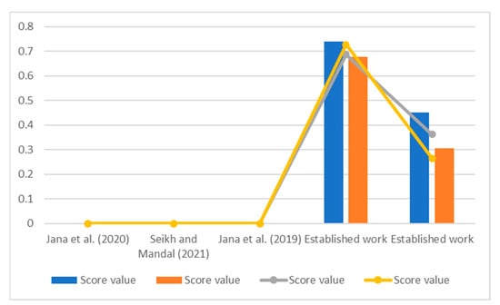
. The graphical depiction of the SVs of the prevailing and proposed operators are displayed in Figure 1

The characteristic comparisons of the existing methods with explored aggregation operators are given in

Table 5. The characteristic comparisons between existing and explored aggregation operators.

Method	Real Part	Imaginary Part	Negative Aspect	Prioritized Relation
BFDWA operator by Jana et al. [34]	Yes	No	Yes	No
BFDWG operator by Jana et al. [34]	Yes	No	Yes	No
IFDWG operator by Seikh and Mandal [21]	Yes	No	No	No
IFDWA operator by Seikh and Mandal [21]	Yes	No	No	No
BFDPWA operator by Jana et al. [33]	Yes	No	Yes	Yes
BFDPWA operator by Jana et al. [33]	Yes	No	Yes	Yes
Established BCFDPWA operator	Yes	No	Yes	Yes
Established BCFDPWA operator	Yes	No	Yes	Yes

.

6. Conclusions

Buildings that are earthquake-resistant must be designed with structural systems because they offer the support and stability needed to withstand seismic forces. Buildings are prone to collapsing without suitable structural systems, which can cause considerable property damage and fatalities. Ground motions produced by earthquakes force the structure to swing and shake. A building’s structural system should be built to withstand the forces produced by these ground motions. This resistance is produced through a variety of structural systems, such as moment-resisting frames, braced frames, and shear walls. The choice of structural system is influenced by several variables, including building height, soil type, and seismicity of the area. Therefore, the selection and prioritization of the finest structural system for earthquake-resistance building is a MADM dilemma. Hence, in this script, we deduced a technique of MADM under BCF information for ranking and assessment of structural systems for earthquake-resistance buildings. For this technique of MADM, we initiated the BCF Dombi prioritized aggregation operators like BCF Dombi prioritized averaging operators, BCF Dombi prioritized weighted averaging operators, BCF Dombi prioritized geometric operators, and BCF Dombi prioritized weighted geometric operators. Afterward, we took hypothetical information in the model of BCFS associated with the structural system for earthquake-resistance buildings and managed a numerical example by employing the developed technique of MADM. We also analyzed the influence of the parameter on the DM outcomes. Finally, we revealed the benefits and dominance of the diagnosed work by comparing the deduced work with the current work.

Future Direction

Due to the importance of the prioritized AO and Dombi operation laws, we hope to spread them to various other modifications of FS, such as bipolar complex intuitionistic fuzzy soft relations [61], bipolar picture FS (BPFS) [62], complex BPFS [63], and bipolar complex spherical fuzzy information [64]. In the future, we would like to do more research on the structure of BCFS.

References

- Grigorian, M.; Sedighi, S.; Targhi, M.A.; Targhi, R.A. Sustainable Earthquake-Resistant Mixed Multiple Seismic Systems. J. Struct. Eng. 2023, 149, 04023002. [Google Scholar] [CrossRef]
- Scalvenzi, M.; Ravasini, S.; Brunesi, E.; Parisi, F. Progressive collapse fragility of substandard and earthquake-resistant precast RC buildings. Eng. Struct. 2023, 275, 115242. [Google Scholar] [CrossRef]
- Maroofi, E.; Mansoori, M.R.; Moghadam, A.S.; Aziminejad, A. Introducing a new seismic resisting system with dual linked column frame and rocking motion. Structures 2023, 47, 2148–2161. [Google Scholar] [CrossRef]
- You, T.; Wang, W.; Tesfamariam, S. Effects of self-centering structural systems on regional seismic resilience. Eng. Struct. 2023, 274, 115125. [Google Scholar] [CrossRef]
- Shi, D. Research and analysis on super high-rise building structure design. In Advances in Civil Function Structure and Industrial Architecture; CRC Press: Boca Raton, FL, USA, 2023; pp. 621–630. [Google Scholar]
- Hanafy, I.M. Fuzzy\beta-Compactness and Fuzzy\beta-Closed Spaces. Turkish J. Math. 2004, 28, 281–294. [Google Scholar]
- Bhavanari, S.; Kuncham, S.P. On fuzzy cosets of Gamma nearrings. Turkish J. Math. 2005, 29, 11–22. [Google Scholar]
- Yun, Y.B.; Kim, K.H.; Öztürk, M.A. Fuzzy maximal ideals of Gamma near-rings. Turkish J. Math. 2001, 25, 457–464. [Google Scholar]
- Zhang, N.; Su, W.; Zhang, C.; Zeng, S. Evaluation and selection model of community group purchase platform based on WEPLPA-CPT-EDAS method. Comput. Ind. Eng. 2022, 172, 108573. [Google Scholar] [CrossRef]
- Atanassov, K. Intuitionistic fuzzy sets. Fuzzy Sets Syst. 1986, 20, 87–96. [Google Scholar] [CrossRef]
- Zadeh, L.A. Fuzzy sets. Inf. Control 1965, 8, 338–353. [Google Scholar] [CrossRef]
- Liu, P.; Liu, J.; Chen, S.M. Some intuitionistic fuzzy Dombi Bonferroni mean operators and their application to multi-attribute group decision making. J. Oper. Res. Soc. 2017, 69, 1–24. [Google Scholar] [CrossRef]
- Zeng, S.; Zhou, J.; Zhang, C.; Merigó, J. Intuitionistic fuzzy social network hybrid MCDM model for an assessment of digital reforms of manufacturing industry in China. Technol. Forecast. Soc. Chang. 2022, 176, 121435. [Google Scholar] [CrossRef]
- Xu, Z.; Yager, R.R. Some geometric aggregation operators based on intuitionistic fuzzy sets. Int. J. Gen. Syst. 2006, 35, 417–433. [Google Scholar] [CrossRef]
- Zhao, H.; Xu, Z.; Ni, M.; Liu, S. Generalized aggregation operators for intuitionistic fuzzy sets. Int. J. Intell. Syst. 2010, 25, 1–30. [Google Scholar] [CrossRef]
- Nguyen, H. A New Aggregation Operator for Intuitionistic Fuzzy Sets with Applications in The Risk Estimation and Decision Making Problem. In Proceedings of the 2020 IEEE International Conference on Fuzzy Systems, Glasgow, UK, 19–24 July 2020; pp. 1–8. [Google Scholar]
- Alcantud, J.C.R.; Khameneh, A.Z.; Kilicman, A. Aggregation of infinite chains of intuitionistic fuzzy sets and their application to choices with temporal intuitionistic fuzzy information. Inf. Sci. 2020, 514, 106–117. [Google Scholar] [CrossRef]
- Xu, Y.; Wang, H. The induced generalized aggregation operators for intuitionistic fuzzy sets and their application in group decision making. Appl. Soft Comput. 2012, 12, 1168–1179. [Google Scholar] [CrossRef]
- Yu, X.; Xu, Z. Prioritized intuitionistic fuzzy aggregation operators. Inf. Fusion 2013, 14, 108–116. [Google Scholar] [CrossRef]
- Yu, D. Multi-Criteria Decision Making Based on Generalized Prioritized Aggregation Operators under Intuitionistic Fuzzy Environment. Int. J. Fuzzy Syst. 2013, 15, 47–54. [Google Scholar]
- Seikh, M.R.; Mandal, U. Intuitionistic fuzzy Dombi aggregation operators and their application to multiple attribute decision-making. Granul. Comput. 2021, 6, 473–488. [Google Scholar] [CrossRef]
- Zeng, S.; Gu, J.; Peng, X. Low-carbon cities comprehensive evaluation method based on Fermatean fuzzy hybrid distance measure and TOPSIS. Artif. Intell. Rev. 2023, 1–17. [Google Scholar] [CrossRef]
- Yang, S.; Pan, Y.; Zeng, S. Decision making framework based Fermatean fuzzy integrated weighted distance and TOPSIS for green low-carbon port evaluation. Eng. Appl. Artif. Intell. 2022, 114, 105048. [Google Scholar] [CrossRef]
- Zhang, W.R. Bipolar fuzzy sets and relations: A computational framework for cognitive modeling and multiagent decision analysis. In Proceedings of the First International Joint Conference of The North American Fuzzy Information Processing Society Biannual Conference. The Industrial Fuzzy Control and Intellige, San Antonio, TX, USA, 18–21 December 1994; pp. 305–309. [Google Scholar]
- Zhang, W.R. (Yin)(Yang) bipolar fuzzy sets. In Proceedings of the 1998 IEEE International Conference on Fuzzy Systems Proceedings, Anchorage, AK, USA, 4–9 May 1998; Volume 1, pp. 840–935. [Google Scholar]
- Lu, M.; Busemeyer, J.R. Do Traditional Chinese Theories of Yi Jing (’Yin-Yang’ and Chinese Medicine Go Beyond Western Concepts of Mind and Matter. Mind. Matter. 2014, 12, 37–59. [Google Scholar]
- Zhang, W.R.; Zhang, J.H.; Shi, Y.; Chen, S.S. Bipolar linear algebra and YinYang-N-element cellular networks for equilibrium-based biosystem simulation and regulation. J. Biol. Syst. 2009, 17, 547–576. [Google Scholar] [CrossRef]
- Zhang, W.R.; Peace, K.E. Causality is logically definable—Toward an equilibrium-based computing paradigm of quantum agents and quantum intelligence (QAQI)(Survey and research). J. Quantum Inf. Sci. 2014, 4, 227–268. [Google Scholar] [CrossRef]
- Zhang, W.R. Bipolar quantum logic gates and quantum cellular combinatorics–a logical extension to quantum entanglement. J. Quantum Inf. Sci. 2013, 3, 93. [Google Scholar] [CrossRef]
- Zhang, W.R. (Ed.) YinYang Bipolar Relativity: A Unifying Theory of Nature, Agents and Causality with Applications in Quantum Computing, Cognitive Informatics and Life Sciences; IGI Global: Hershey, PA, USA, 2011. [Google Scholar]
- Zhang, W.R.; Pandurangi, A.K.; Peace, K.E.; Zhang, Y.Q.; Zhao, Z. MentalSquares: A generic bipolar support vector machine for psychiatric disorder classification, diagnostic analysis and neurobiological data mining. Int. J. Data Min. Bioinform. 2011, 5, 532–557. [Google Scholar] [CrossRef]
- Gul, Z. Some Bipolar Fuzzy Aggregations Operators and Their Applications in Multicriteria Group Decision Making. Ph.D. Thesis, Hazara University, Mansehra, Pakistan, 2015. [Google Scholar]
- Jana, C.; Pal, M.; Wang, J.Q. Bipolar fuzzy Dombi prioritized aggregation operators in multiple attribute decision making. Soft Comput. 2020, 24, 3631–3646. [Google Scholar] [CrossRef]
- Jana, C.; Pal, M.; Wang, J.Q. Bipolar fuzzy Dombi aggregation operators and its application in multiple-attribute decision-making process. J. Ambient Intell. Human. Comput. 2019, 10, 3533–3549. [Google Scholar] [CrossRef]
- Gao, H.; Wei, G.; Huang, Y. Dual hesitant bipolar fuzzy Hamacher prioritized aggregation operators in multiple attribute decision making. IEEE Access 2017, 6, 11508–11522. [Google Scholar] [CrossRef]
- Wei, G.; Alsaadi, F.E.; Hayat, T.; Alsaedi, A. Bipolar fuzzy Hamacher aggregation operators in multiple attribute decision making. Int. J. Fuzzy Syst. 2018, 20, 1–12. [Google Scholar] [CrossRef]
- Abdullah, S.; Aslam, M.; Ullah, K. Bipolar fuzzy soft sets and its applications in decision making problem. J. Intell. Fuzzy Syst. 2014, 27, 729–742. [Google Scholar] [CrossRef]
- Jana, C.; Pal, M.; Wang, J. A robust aggregation operator for multi-criteria decision-making method with bipolar fuzzy soft environment. Iran. J. Fuzzy Syst. 2019, 16, 1–16. [Google Scholar]
- Mustafa, H.I. Bipolar soft ideal rough set with applications in COVID-19. Turkish J. Math. 2023, 47, 1–36. [Google Scholar] [CrossRef]
- Ramot, D.; Milo, R.; Friedman, M.; Kandel, A. Complex fuzzy sets. IEEE Trans. Fuzzy Syst. 2002, 10, 171–186. [Google Scholar] [CrossRef]
- Tamir, D.E.; Jin, L.; Kandel, A. A new interpretation of complex membership grade. Int. J. Intell. Syst. 2011, 26, 285–312. [Google Scholar] [CrossRef]
- Zhang, G.; Dillon, T.S.; Cai, K.Y.; Ma, J.; Lu, J. Operation properties and δ-equalities of complex fuzzy sets. Int. J. Approx. Reason. 2009, 50, 1227–1249. [Google Scholar] [CrossRef]
- Ramot, D.; Friedman, M.; Langholz, G.; Kandel, A. Complex fuzzy logic. IEEE Trans. Fuzzy Syst. 2003, 11, 450–461. [Google Scholar] [CrossRef]
- Greenfield, S.; Chiclana, F.; Dick, S. Interval-valued complex fuzzy logic. In Proceedings of the 2016 IEEE International Conference on Fuzzy Systems (FUZZ-IEEE), Vancouver, BC, Canada, 24–29 July 2016; pp. 2014–2019. [Google Scholar]
- Tamir, D.E.; Rishe, N.D.; Kandel, A. Complex fuzzy sets and complex fuzzy logic an overview of theory and applications. In Fifty Years of Fuzzy Logic and Its Applications. Studies in Fuzziness and Soft Computing; Springer: Cham, Switzerland, 2015; Volume 26, pp. 661–681. [Google Scholar]
- Yazdanbakhsh, O.; Dick, S. A systematic review of complex fuzzy sets and logic. Fuzzy Sets Syst. 2018, 338, 1–22. [Google Scholar] [CrossRef]
- Bi, L.; Dai, S.; Hu, B.; Li, S. Complex fuzzy arithmetic aggregation operators. J. Intell. Fuzzy Syst. 2019, 36, 2765–2771. [Google Scholar] [CrossRef]
- Bi, L.; Dai, S.; Hu, B. Complex fuzzy geometric aggregation operators. Symmetry 2018, 10, 251. [Google Scholar] [CrossRef]
- Dai, S.; Bi, L.; Hu, B. Interval-valued complex fuzzy geometric aggregation operators and their application to decision making. Math. Probl. Eng. 2020, 2020, 9410143. [Google Scholar] [CrossRef]
- Hu, B.; Bi, L.; Dai, S. Complex Fuzzy Power Aggregation Operators. Math. Probl. Eng. 2019, 2019, 9064385. [Google Scholar] [CrossRef]
- Mahmood, T.; Ur Rehman, U. A novel approach towards bipolar complex fuzzy sets and their applications in generalized similarity measures. Int. J. Intell. Syst. 2022, 37, 535–567. [Google Scholar] [CrossRef]
- Mahmood, T.; Rehman, U.U.; Ahmmad, J.; Santos-García, G. Bipolar complex fuzzy Hamacher aggregation operators and their applications in multi-attribute decision making. Mathematics 2021, 10, 23. [Google Scholar] [CrossRef]
- Mahmood, T.; Rehman, U.U. A method to multi-attribute decision making technique based on Dombi aggregation operators under bipolar complex fuzzy information. Comput. Appl. Math. 2022, 41, 47. [Google Scholar] [CrossRef]
- Mahmood, T.; ur Rehman, U.; Ali, Z. Analysis and application of Aczel-Alsina aggregation operators based on bipolar complex fuzzy information in multiple attribute decision making. Inf. Sci. 2023, 619, 817–833. [Google Scholar] [CrossRef]
- Mahmood, T.; Rehman, U.U.; Ali, Z.; Aslam, M.; Chinram, R. Identification and classification of aggregation operators using bipolar complex fuzzy settings and their application in decision support systems. Mathematics 2022, 10, 1726. [Google Scholar] [CrossRef]
- Rehman, U.U.; Mahmood, T.; Albaity, M.; Hayat, K.; Ali, Z. Identification and Prioritization of DevOps Success Factors Using Bipolar Complex Fuzzy Setting with Frank Aggregation Operators and Analytical Hierarchy Process. IEEE Access 2022, 10, 74702–74721. [Google Scholar] [CrossRef]
- Yager, R.R.; Kacprzyk, J. The Ordered Weighted Averaging Operators: Theory and Applications; Springer Science & Business Media: Berlin, Germany, 2012. [Google Scholar]
- Yager, R.R. Prioritized aggregation operators. Int. J. Approx. Reason. 2008, 48, 263–274. [Google Scholar] [CrossRef]
- Xu, Z.; Da, Q.L. An overview of operators for aggregating information. Int. J. Intell. Syst. 2003, 18, 953–969. [Google Scholar] [CrossRef]
- Dombi, J. A general class of fuzzy operators, the DeMorgan class of fuzzy operators and fuzziness measures induced by fuzzy operators. Fuzzy Sets Syst. 1982, 8, 149–163. [Google Scholar] [CrossRef]
- Gwak, J.; Garg, H.; Jan, N. Investigation of Robotics Technology Based on Bipolar Complex Intuitionistic Fuzzy Soft Relation. Int. J. Fuzzy Syst. 2023, 1–19. [Google Scholar] [CrossRef]
- Khan, W.A.; Faiz, K.; Taouti, A. Bipolar picture fuzzy sets and relations with applications. Songklanakarin J. Sci. Technol. 2022, 44, 987–999. [Google Scholar]
- Jan, N.; Akram, B.; Nasir, A.; Alhilal, M.S.; Alabrah, A.; Al-Aidroos, N. An innovative approach to investigate the effects of artificial intelligence based on complex bipolar picture fuzzy information. Sci. Program. 2022, 2022, 1460544. [Google Scholar] [CrossRef]
- Gwak, J.; Garg, H.; Jan, N.; Akram, B. A new approach to investigate the effects of artificial neural networks based on bipolar complex spherical fuzzy information. Complex Intell. Syst. 2023, 1–24. [Google Scholar] [CrossRef]
Disclaimer/Publisher’s Note: The statements, opinions and data contained in all publications are solely those of the individual author(s) and contributor(s) and not of MDPI and/or the editor(s). MDPI and/or the editor(s) disclaim responsibility for any injury to people or property resulting from any ideas, methods, instructions or products referred to in the content. |
© 2023 by the authors. Licensee MDPI, Basel, Switzerland. This article is an open access article distributed under the terms and conditions of the Creative Commons Attribution (CC BY) license (https://creativecommons.org/licenses/by/4.0/).