Mylar Balloon and Associated Geometro-Mechanical Moments

Abstract

Starting with identifications of the very fundamental geometric characteristics of a Mylar balloon such as the profile curve, height, volume, arclength, surface area, crimping factor, etc., using the geometrical moments $I_n\left(x\right)$ and $I_n$, we present explicit formulas for them and those of the mechanical moments of both solid and hollow balloons of arbitrary order. This is achieved by relying on the recursive relationships among elliptic integrals and the final results are expressed via the fundamental mathematical constants such as $\pi$, lemniscate constant $\tilde{\omega }$, and Gauss’s constant G. An interesting periodicity modulo 4 was detected and accounted for in the final formulas for the moments. The principal results are illustrated by two tables, a few graphics, and some direct relationships with other fundamental areas in mathematics, physics and geometry are pointed out.

1. Introduction

Before focusing on the actual contents of the paper the reader might be interested to learn something about the Mylar balloon itself. According to Webster’s New World Dictionary, Mylar is an Americanism meaning a trademark for a polyester made in extremely thin sheets of great tensile strength. This term has been introduced by Paulsen [1] in the form of a variational problem under a constraint and with an idea to replace the so-called e-balloon explored intensively in the 70s by NASA (cf., e.g., [2]). More detail about the present day situation with the zero-pressure balloons can be found in [3].

According to Paulsen the Mylar balloon is constructed by taking two identical circular disks of Mylar, sewing them together along their boundaries, and then inflating the resulting object with either air or helium. Surprisingly enough, these balloons turn out not to be spherical as one might expect based on the well-known fact that the sphere possesses the maximal volume for a given surface area. Respectively, this purely experimental fact suggests the following mathematical problem: given a circular Mylar balloon of deflated radius a, what will be the shape of the balloon when it is fully inflated (i.e., inflated to maximize the volume subject to the constraint that the Mylar does not stretch)?

It should be also noted that the Japanese engineer Kawaguchi [4] had arrived at the same figure when looking for a shallowest surface of revolution which has no circumferential stress. This is achieved exactly when the meridional $k_{\mu }$ and parallel $k_{\pi }$ principal curvatures obey everywhere the condition

$$k_{\mu }=2k_{\pi }.$$

(1)

Some years later Mladenov and Oprea [5] proved that this linear-type relationship between curvatures specifies the rotational surfaces uniquely.

The rest of the paper is organized as follows. In Section 2 the geometrical moments $I_n\left(x\right)$ and $I_n$ are defined and it is shown how the main characteristics of the Mylar balloon can be expressed via them. In Section 3 the mechanical moments $J_n$ and ${\stackrel{\circ }{J}}_n$ of the solid and hollow Mylar balloons are studied and it is shown that in both considered cases they can be connected to the geometrical moments $I_n$. Section 4 is devoted to investigation of the recurrent relations (modulo 4) for the sequence of the geometrical moments $I_n\left(x\right)$ and $I_n$, while in Section 5 the corresponding residue classes of the mechanical moments $J_n$ and ${\stackrel{\circ }{J}}_n$ for the solid and hollow Mylar balloons are shown and the first twenty values of the numerical coefficients ${\mu }_n$ and ${\stackrel{\circ }{\mu }}_n$ are calculated explicitly via Gauss’s constant G with the aid of the Wolfram computer language using the symbolic computation program Mathematica^® [6]. Finally, Section 6 concludes the paper and points out a possible direction for the related future work. The main new results of the presented research can be found in Section 2, Section 3, Section 4 and Section 5. The paper deals with the fundamental problem which appears at least in Celestial Mechanics, Probability Theory and Statistics and could help significantly in other areas where one needs to account for corrections keeping some control over them.

2. Balloon’s Characteristics Expressed via Geometrical Moments

The Mylar balloon (see Figure 1) can be defined as a surface of revolution that is obtained when we maximize the volume V (no stretching of the Mylar foil is allowed) for a given (fixed) arclength $L\equiv a$ (where a is the radius of the deflated Mylar balloon, i.e., of the Mylar discs) of its profile curve (i.e., the directrix that generates the surface) $z=z\left(x\right)$ for x changing from $x=0$ to $x=r$, where r is the radius of the inflated Mylar balloon, and obviously we have $r<a$ (see, e.g., [1,7,8]).

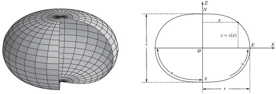
Figure 1. 3D view of the inflated Mylar balloon (left) and its cross-section through the symmetry axis $OZ$ in the plane $XOZ$ (right). N and S are the North and South Poles, E denotes the Equator of this surface of revolution, and O is the center of the Mylar balloon. The profile curve is defined through the relation $z=z\left(x\right)$, whereas $\tau =2z\left(0\right)$ is the thickness of the Mylar balloon and a, r are its deflated and inflated radii, respectively. Alternatively, the variable u describes the parametrization of the Mylar balloon, i.e., $x=x\left(u\right)$ and $z=z\left(u\right)$ with $u\in [-1,1]$.

It can be shown that the constraint equation for the profile curve can be written as

$$z^{\prime }\left(x\right)=-\frac{x^2}{\sqrt{r^4-x^4}},\mathrm{i}.\mathrm{e}.,z\left(x\right)=\underset{x}{\overset{r}{\int }}\frac{t^2\mathrm{d}t}{\sqrt{r^4-t^4}}x\in [0,r].$$

(2)

Therefore, the height, volume, and arclength of the Mylar balloon can be found, respectively, as

$$\tau =2z\left(0\right)=2\underset{0}{\overset{r}{\int }}\frac{t^2\mathrm{d}t}{\sqrt{r^4-t^4}},V=2\pi \underset{0}{\overset{r}{\int }}\frac{t^4\mathrm{d}t}{\sqrt{r^4-t^4}},L=r^2\underset{0}{\overset{r}{\int }}\frac{\mathrm{d}t}{\sqrt{r^4-t^4}}\equiv a.$$

(3)

Similarly, we can calculate the surface area of the inflated Mylar balloon by integrating over all the circular strips of the surface of revolution with the length $2\pi x$, where x is the distance to the axis of rotation, and the infinitesimal width $\mathrm{d}s$, where $\mathrm{d}{s}^2=\mathrm{d}{x}^2+\mathrm{d}{z}^2$, i.e.,

$$S_{\mathrm{inflated}}=2\pi \int x\mathrm{d}s=2\pi \int x\sqrt{\mathrm{d}{x}^2+\mathrm{d}{z}^2}=4\pi \underset{x=0}{\overset{r}{\int }}x\sqrt{1+{\left(z^{\prime }\left(x\right)\right)}^2}\mathrm{d}x$$

(4)

where we can substitute the expression for the derivative $z^{\prime }\left(x\right)$ given in (2) and obtain

$$S_{\mathrm{inflated}}=2\pi r^2\underset{0}{\overset{r}{\int }}\frac{\mathrm{d}\left(x^2\right)}{\sqrt{r^4-x^4}}=2\pi r^2{\left.arcsin\frac{x^2}{r^2}\right|}_0^r={\pi }^2{r}^2.$$

(5)

We can see that the above surface area clearly differs from the surface area of the two sewn-together circular Mylar discs of radius a, i.e., $S_{\mathrm{deflated}}=2\pi a^2$, describing effective shrinking of the inflated Mylar balloon’s surface compared to the deflated one

$$\frac{S_{\mathrm{deflated}}}{S_{\mathrm{inflated}}}=\frac{2}{\pi }{\left(\frac{a}{r}\right)}^2\approx 1.09422.$$

(6)

We can also introduce the local measure of the above-described shrinking that is defined as the ratio of the surface area of a small patch on the deflated Mylar balloon to the surface area of the corresponding patch on the inflated Mylar balloon. This local measure is called the crimping factor and is defined through the relation (see, e.g., [1])

$$C\left(x\right)=\frac{r^2}{x}\underset{0}{\overset{x}{\int }}\frac{\mathrm{d}t}{\sqrt{r^4-t^4}}·$$

(7)

It can be shown that the crimping factor is minimal for $x=0$ (see Figure 2–right), i.e.,

$$C_{\min }=C\left(0\right)=\underset{x\to 0}{lim}\frac{r^2}{x}\underset{0}{\overset{x}{\int }}\frac{\mathrm{d}t}{\sqrt{r^4-t^4}}={\left[\frac{0}{0}\right]}_{\mathrm{L’}\mathrm{H}\widehat{\mathrm{o}}\mathrm{spital’s}\mathrm{rule}}=\underset{x\to 0}{lim}\frac{r^2}{\sqrt{r^4-x^4}}=1$$

(8)

and maximal for $x=r$ (again see Figure 2–right), i.e.,

$$C_{\max }=C\left(r\right)=r\underset{0}{\overset{r}{\int }}\frac{\mathrm{d}t}{\sqrt{r^4-t^4}}=\frac{L}{r}\equiv \frac{a}{r}\approx 1.31103.$$

(9)

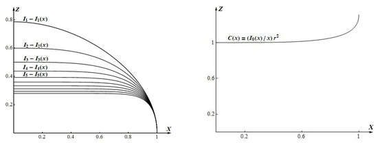
Figure 2. Dependencies of $I_n-I_n\left(x\right)$, $n=1,\dots ,10$ (left, top to bottom), including the profile curve $z\left(x\right)=I_2-I_2\left(x\right)$, and the crimping factor $C\left(x\right)$ (right), for the Mylar balloon with radius $r=1$.

Therefore, we can see that all the above relations clearly indicate that the Mylar balloon can be actually characterized by the set of geometrical moments that are defined as

$$I_n\left(x\right):=\underset{0}{\overset{x}{\int }}\frac{t^n\mathrm{d}t}{\sqrt{r^4-t^4}},I_n:=I_n\left(r\right),I_n\left(0\right)=0,n=0,1,2,\dots$$

(10)

Then we can write down the above formulas in the alternative forms, i.e., $z\left(x\right)=I_2-I_2\left(x\right)$, $\tau =2I_2$, $V=2\pi I_4$, $L=r^2{I}_0\equiv a$, $S_{\mathrm{inflated}}={\pi }^2{r}^2=4\pi r^2{I}_1$, and $C\left(x\right)=(r^2/x)I_0\left(x\right)$.

Finally, the explicit parametrization ($u\in [-1,1]$) of the inflated Mylar balloon’s profile curve (directrix) can be obtained from (2) as (see, e.g., [9])

$$\begin{array}{ccc}\hfill x\left(u\right)& =& r\sqrt{\frac{1-u^2}{1+u^2}}\hfill \end{array}$$

(11)

$$\begin{array}{ccc}\hfill z\left(u\right)& =& \frac{r}{\sqrt{2}}\left(2E\left(arcsin\frac{\sqrt{2}u}{\sqrt{1+u^2}},\frac{1}{\sqrt{2}}\right)-F\left(arcsin\frac{\sqrt{2}u}{\sqrt{1+u^2}},\frac{1}{\sqrt{2}}\right)\right)\hfill \end{array}$$

(12)

where $F(\phi ,k)$ and $E(\phi ,k)$ denote the incomplete elliptic integrals of the first and second kind with the Jacobian amplitude $\phi$ and elliptic modulus k (see, e.g., [10]). From (11) and (12) we can also obtain the explicit dependency $z\left(x\right)$ that is given as (see Figure 1)

$$z\left(x\right)=\frac{r}{\sqrt{2}}\left(2E\left(arccos\frac{x}{r},\frac{1}{\sqrt{2}}\right)-F\left(arccos\frac{x}{r},\frac{1}{\sqrt{2}}\right)\right).$$

(13)

3. Mechanical Moments of Solid and Hollow Mylar Balloons

It is well known that in order to determine the attraction between gravitating bodies one needs to know the inertia moments of arbitrary order. In most of the astronomical applications only a few of them are used. However, if the difference in masses is significant and the space in which the bodies are considered is confined, the higher moments are essential as well. This holds definitely in the case of the motion around the oblate primary [11]. Strangely enough, the higher moments appear in probability and statistics (cf. [12]) where at least the first six of them have specific names.

In our setting specifically, we suppose that either the volume or the surface area of the Mylar balloon is filled with the physical material of the total mass m that has the homogeneous distribution of the mass (i.e., the constant density). Thus, in the first case we will obtain the solid Mylar balloon (with the constant volumetric mass density $\rho =m/V$), whereas in the second case it will be the hollow Mylar balloon (with the constant surface mass density $\stackrel{\circ }{\rho }=m/S_{\mathrm{inflated}}$).

For such two (solid and hollow) physical realizations of the Mylar balloon we can define the corresponding mechanical moments of mass calculated with respect to the vertical axis of symmetry of the described surface of revolution as

$$J_n=\underset{V}{\int \int \int }{x}^n\mathrm{d}{\mu }_V=\rho \underset{V}{\int \int \int }{x}^n\mathrm{d}V,{\stackrel{\circ }{J}}_n=\underset{S_{\mathrm{inflated}}}{\int \int }{x}^n\mathrm{d}{\mu }_S=\stackrel{\circ }{\rho }\underset{S_{\mathrm{inflated}}}{\int \int }{x}^n\mathrm{d}S,n=0,1,2,\dots$$

(14)

where x is the distance from the vertical axis of symmetry to the infinitesimal mass $\mathrm{d}\mu$ that is positioned either in the volume or on the surface of the Mylar balloon, ${\mu }_V$ and ${\mu }_S$ are the corresponding measures of the volumetric and surface mass distributions, and the circle indicates that the respective quantities are associated with the hollow Mylar balloon.

Hence, the zeroth (monopole) and second (quadrupole) mechanical moments of mass will correspond to the total mass (the same by construction in both cases) and two polar moments of inertia for the solid and hollow Mylar balloons respectively, i.e.,

$$J_0={\stackrel{\circ }{J}}_0=m,J_2=M=\rho \underset{V}{\int \int \int }{x}^2\mathrm{d}V,{\stackrel{\circ }{J}}_2=\stackrel{\circ }{M}=\stackrel{\circ }{\rho }\underset{S_{\mathrm{inflated}}}{\int \int }{x}^2\mathrm{d}S.$$

(15)

3.1. Mechanical Moments of Solid Mylar Balloon

Using cylindrical coordinates $(x,z,\theta )$, where $\theta \in [0,2\pi ]$, and taking into account the symmetry of the Mylar balloon with respect to the equatorial ($XOY$) plane (see Figure 1) the mechanical moments $J_n$ given by the first expression in (14) can be rewritten as

$$J_n=2\rho \underset{x=0}{\overset{r}{\int }}\underset{z=0}{\overset{z\left(x\right)}{\int }}\underset{\theta =0}{\overset{2\pi }{\int }}{x}^{n+1}\mathrm{d}\theta \mathrm{d}z\mathrm{d}x=4\pi \rho \underset{x=0}{\overset{r}{\int }}{x}^{n+1}z\left(x\right)\mathrm{d}x=4\pi \rho \underset{x=0}{\overset{r}{\int }}\underset{t=x}{\overset{r}{\int }}\frac{x^{n+1}{t}^2}{\sqrt{r^4-t^4}}\mathrm{d}t\mathrm{d}x$$

(16)

where we have used the integral representation (2) of the expression $z\left(x\right)$. After changing the order of integration (from $(x,t)\in [0,r]\times [x,r]$ to $(t,x)\in [0,r]\times [0,t]$) we obtain

$$J_n=4\pi \rho \underset{t=0}{\overset{r}{\int }}\underset{x=0}{\overset{t}{\int }}\frac{t^2{x}^{n+1}}{\sqrt{r^4-t^4}}\mathrm{d}x\mathrm{d}t=\frac{4\pi \rho }{n+2}\underset{t=0}{\overset{r}{\int }}\frac{t^{n+4}\mathrm{d}t}{\sqrt{r^4-t^4}}=\frac{4\pi \rho }{n+2}{I}_{n+4}$$

(17)

i.e., the mechanical moments $J_n$ can be expressed through the geometrical moments $I_{n+4}$ given by (10). It also turns out to be convenient to represent $J_n$ in the form

$$J_n={\mu }_{n}m{r}^n,m=\rho V=2\pi \rho I_4=J_0,{\mu }_n=\frac{2}{n+2}·\frac{I_{n+4}}{I_4}·\frac{1}{r^n}$$

(18)

where ${\mu }_n$ are the numerical coefficients that will be explicitly evaluated in Section 5.

3.2. Mechanical Moments of Hollow Mylar Balloon

Similarly to the solid case from the previous section, for the hollow Mylar balloon we can rewrite the mechanical moments ${\stackrel{\circ }{J}}_n$ given by the second expression in (14) as

$${\stackrel{\circ }{J}}_n=2\stackrel{\circ }{\rho }\underset{x=0}{\overset{r}{\int }}\underset{\theta =0}{\overset{2\pi }{\int }}{x}^{n+1}\sqrt{1+{\left(z^{\prime }\left(x\right)\right)}^2}\mathrm{d}x\mathrm{d}\theta =4\pi r^2\stackrel{\circ }{\rho }\underset{x=0}{\overset{r}{\int }}\frac{x^{n+1}\mathrm{d}x}{\sqrt{r^4-x^4}}=4\pi r^2\stackrel{\circ }{\rho }{I}_{n+1}$$

(19)

where we have used the expression for the derivative $z^{\prime }\left(x\right)$ given in (2).

As we can see, for the hollow Mylar balloon the mechanical moments ${\stackrel{\circ }{J}}_n$ can be expressed through the geometrical moments $I_{n+1}$ and it is convenient to represent them as

$${\stackrel{\circ }{J}}_n={\stackrel{\circ }{\mu }}_{n}m{r}^n,m=\stackrel{\circ }{\rho }{S}_{\mathrm{inflated}}={\pi }^2{r}^2\stackrel{\circ }{\rho }=4\pi r^2\stackrel{\circ }{\rho }{I}_1={\stackrel{\circ }{J}}_0,{\stackrel{\circ }{\mu }}_n=\frac{4}{\pi }\frac{I_{n+1}}{r^n}=\frac{I_{n+1}}{I_1}·\frac{1}{r^n}$$

(20)

where the numerical coefficients ${\stackrel{\circ }{\mu }}_n$ will be again explicitly evaluated in Section 5.

4. Recursive Evaluation of Geometrical Moments ${\mathit{I}}_{\mathit{n}}\left(\mathit{x}\right)$ and ${\mathit{I}}_{\mathit{n}}$

In order to obtain the recursive formula for the geometrical moments $I_n\left(x\right)$ given by (10) we can use the expression (cf., e.g., [13] Formula (250.01)).

$$I_{n+4}\left(x\right)=\frac{n+1}{n+3}{I}_n\left(x\right)r^4-\frac{x^{n+1}}{n+3}\sqrt{r^4-x^4},n=0,1,2,\dots$$

(21)

or we can reobtain it directly using integration by parts and the differential relation

$$\frac{t^3\mathrm{d}t}{\sqrt{r^4-t^4}}=-\frac{1}{2}\mathrm{d}\left(\sqrt{r^4-t^4}\right).$$

(22)

Then the first integral expression in (10) taken for $n+4$ can be rewritten in the form

$$I_{n+4}\left(x\right)=-\frac{1}{2}\underset{0}{\overset{x}{\int }}{t}^{n+1}\mathrm{d}\left(\sqrt{r^4-t^4}\right)=-{\left.\frac{t^{n+1}}{2}\sqrt{r^4-t^4}\right|}_0^x+\frac{n+1}{2}\underset{0}{\overset{x}{\int }}{t}^n\sqrt{r^4-t^4}\mathrm{d}t$$

(23)

where after interpreting the last integral as $r^4{I}_n\left(x\right)-I_{n+4}\left(x\right)$ we reobtain (21) for $n\ge 0$.

Hence, using the explicit representations of the first four geometrical moments $I_n\left(x\right)$ (for the dependencies, $I_n-I_n\left(x\right)$, see Figure 2–left; for the values of $I_n$, see (30)–(38)), i.e.,

$$\begin{array}{ccc}\hfill I_0\left(x\right)& =& \frac{1}{\sqrt{2}}\left(K\left(\frac{1}{\sqrt{2}}\right)-F\left(arccos\frac{x}{r},\frac{1}{\sqrt{2}}\right)\right)·\frac{1}{r}\hfill \end{array}$$

(24)

$$\begin{array}{ccc}\hfill I_1\left(x\right)& =& \frac{1}{2}arcsin\frac{x^2}{r^2}\hfill \end{array}$$

(25)

$$\begin{array}{ccc}\hfill I_2\left(x\right)& =& \frac{1}{\sqrt{2}}\left(2E\left(\frac{1}{\sqrt{2}}\right)-K\left(\frac{1}{\sqrt{2}}\right)-2E\left(arccos\frac{x}{r},\frac{1}{\sqrt{2}}\right)+F\left(arccos\frac{x}{r},\frac{1}{\sqrt{2}}\right)\right)·r\hfill \end{array}$$

(26)

$$\begin{array}{ccc}\hfill I_3\left(x\right)& =& \frac{1}{2}\left(1-\sqrt{1-\frac{x^4}{r^4}}\right)·r^2\hfill \end{array}$$

(27)

and the expression (21) we can obtain all the geometrical moments $I_n\left(x\right)$ for $n\ge 0$, e.g., the next two are given as

$$\begin{array}{ccc}\hfill I_4\left(x\right)& =& \frac{1}{3}\left(\frac{1}{\sqrt{2}}\left(K\left(\frac{1}{\sqrt{2}}\right)-F\left(arccos\frac{x}{r},\frac{1}{\sqrt{2}}\right)\right)-\frac{x}{r}\sqrt{1-\frac{x^4}{r^4}}\right)·r^3\hfill \end{array}$$

(28)

$$\begin{array}{ccc}\hfill I_5\left(x\right)& =& \frac{1}{4}\left(arcsin\frac{x^2}{r^2}-\frac{x^2}{r^2}\sqrt{1-\frac{x^4}{r^4}}\right)·r^4\hfill \end{array}$$

(29)

where $F(\phi ,k)$ and $E(\phi ,k)$ denote the incomplete elliptic integrals of the first and second kind with the Jacobian amplitude $\phi$ and elliptic modulus k, whereas $K\left(k\right)=F(\pi /2,k)$ and $E\left(k\right)=E(\pi /2,k)$ are the complete elliptic integrals of the first and second kind (see [10]).

The corresponding values of the first four geometrical moments $I_n$ are given as

$$\begin{array}{ccc}\hfill I_0& =& \frac{1}{\sqrt{2}}K\left(\frac{1}{\sqrt{2}}\right)·\frac{1}{r}\approx 1.31101·\frac{1}{r}\hfill \end{array}$$

(30)

$$\begin{array}{ccc}\hfill I_1& =& \frac{\pi }{4}\approx 0.785398\hfill \end{array}$$

(31)

$$\begin{array}{ccc}\hfill I_2& =& \frac{1}{\sqrt{2}}\left(2E\left(\frac{1}{\sqrt{2}}\right)-K\left(\frac{1}{\sqrt{2}}\right)\right)·r\approx 0.59907·r\hfill \end{array}$$

(32)

$$\begin{array}{ccc}\hfill I_3& =& \frac{1}{2}·r^2=0.5·r^2\hfill \end{array}$$

(33)

whereas the rest of them for all values $n\ge 0$ can be calculated using the recursive relation

$$I_{n+4}=\frac{n+1}{n+3}{I}_n{r}^4$$

(34)

e.g., the next four geometrical moments are given as

$$\begin{array}{ccc}\hfill I_4& =& \frac{1}{3}{I}_0{r}^4=\frac{1}{3\sqrt{2}}K\left(\frac{1}{\sqrt{2}}\right)·r^3\approx 0.43701·r^3\hfill \end{array}$$

(35)

$$\begin{array}{ccc}\hfill I_5& =& \frac{1}{2}{I}_1{r}^4=\frac{\pi }{8}·r^4\approx 0.392699·r^4\hfill \end{array}$$

(36)

$$\begin{array}{ccc}\hfill I_6& =& \frac{3}{5}{I}_2{r}^4=\frac{3}{5\sqrt{2}}\left(2E\left(\frac{1}{\sqrt{2}}\right)-K\left(\frac{1}{\sqrt{2}}\right)\right)·r^5\approx 0.359442·r^5\hfill \end{array}$$

(37)

$$\begin{array}{ccc}\hfill I_7& =& \frac{2}{3}{I}_3{r}^4=\frac{1}{3}·r^6\approx 0.333333·r^6.\hfill \end{array}$$

(38)

By applying (34) iteratively for $n\equiv p\left(\mathrm{mod}4\right)$, $p=\{0,1,2,3\}$, i.e., for each of the four residue classes $n|p$, it can be readily obtained that

$$I_{n+4|p}=\frac{(n+1)!!!!}{(n+3)!!!!}{I}_p{r}^{n+4-p}$$

(39)

where the shortcut notation $n!!!!$ stands for the quadruple factorial, i.e., a product of positive integers defined by the formula $n!!!!=n(n-4)(n-8)(n-12)\dots$ It can be easily seen that, when n is an even number, i.e., when $n=2k$ with $k\ge 0$, then $n!!!!=2^{k}k!!$, where $k!!$ stands for the double factorial, i.e., a product of positive integers defined by the formula $k!!=k(k-2)(k-4)(k-6)\dots$

Finally, let us present some exemplary calculations of the characteristics of the Mylar balloon expressed through the geometrical moments $I_n\left(x\right)$ presented in Section 2, i.e., the profile curve $z\left(x\right)$ and the crimping factor $C\left(x\right)$ are given as (see Figure 2–left for $z\left(x\right)=I_2-I_2\left(x\right)$, right for $C\left(x\right)$)

$$\begin{array}{ccc}\hfill z\left(x\right)& =& I_2-I_2\left(x\right)=\frac{r}{\sqrt{2}}\left(2E\left(arccos\frac{x}{r},\frac{1}{\sqrt{2}}\right)-F\left(arccos\frac{x}{r},\frac{1}{\sqrt{2}}\right)\right)\hfill \end{array}$$

(40)

$$\begin{array}{ccc}\hfill C\left(x\right)& =& \frac{I_0\left(x\right)}{x}·r^2=\frac{r}{x\sqrt{2}}\left(K\left(\frac{1}{\sqrt{2}}\right)-F\left(arccos\frac{x}{r},\frac{1}{\sqrt{2}}\right)\right)\hfill \end{array}$$

(41)

(the first expression is identical to the parametrization (13) of the Mylar balloon), whereas the arclength L, equivalently, deflated radius a, height $\tau$, and volume V are calculated as

$$\begin{array}{ccc}\hfill L\equiv a& =& I_0{r}^2=\frac{1}{\sqrt{2}}K\left(\frac{1}{\sqrt{2}}\right)·r\approx 1.31101·r\hfill \end{array}$$

(42)

$$\begin{array}{ccc}\hfill \tau & =& 2I_2=\sqrt{2}\left(2E\left(\frac{1}{\sqrt{2}}\right)-K\left(\frac{1}{\sqrt{2}}\right)\right)·r\approx 1.19814·r\hfill \end{array}$$

(43)

$$\begin{array}{ccc}\hfill V& =& 2\pi I_4=\frac{2\pi }{3}{I}_0{r}^4=\frac{\sqrt{2}\pi }{3}K\left(\frac{1}{\sqrt{2}}\right)·r^3\approx 2.74581·r^3.\hfill \end{array}$$

(44)

5. Residue Classes Modulo 4 of Mechanical Moments

By making use of the recursive Formula (39) for the geometrical moments $I_n$ for $n\ge 0$, we can arrive at an explicit representation of the mechanical moments $J_n$ given by (18) and ${\stackrel{\circ }{J}}_n$ given by (20) classifying them into four non-intersecting residue classes $J_{n|p}$ as

$$J_{n|p}={\mu }_{n|p}m{r}^n,{\stackrel{\circ }{J}}_{n|p}={\stackrel{\circ }{\mu }}_{n|p}m{r}^n,n\equiv p\left(\mathrm{mod}4\right),p=\{0,1,2,3\}.$$

(45)

In the next two sections we will discuss in detail the recursive calculation of the numerical coefficients ${\mu }_{n|p}$ and ${\stackrel{\circ }{\mu }}_{n|p}$ for the cases of the solid and hollow Mylar balloons. Most of the calculations were made by the aid of the Wolfram computer language using the Computer Algebra System Mathematica^® [6].

5.1. Calculation of Numerical Coefficients ${\mu }_n$ for Solid Mylar Balloon

For the solid Mylar balloon the numerical coefficients ${\mu }_{n|p}$ given by (18) using the recursive Formula (39) can be calculated as

$${\mu }_{n|p}=\frac{2}{n+2}·\frac{I_{n+4|p}}{I_4}·\frac{1}{r^n}=\frac{6}{n+2}·\frac{I_{n+4|p}}{I_0}·\frac{1}{r^{n+4}}=\frac{6}{n+2}·\frac{(n+1)!!!!}{(n+3)!!!!}·\frac{I_p}{I_0}·\frac{1}{r^p}$$

(46)

or substituting directly the values of $I_p$, $p=\{0,1,2,3\}$, given by (30)–(33) we obtain

$$\begin{array}{ccc}\hfill {\mu }_{4k+0}& =& \frac{3}{2k+1}·\frac{(4k+1)!!!!}{(4k+3)!!!!}·\frac{I_0}{I_0}=\frac{3}{2k+1}·\frac{1}{3}·\frac{5}{7}·\frac{9}{11}\cdots \frac{4k+1}{4k+3}·1\hfill \end{array}$$

(47)

$$\begin{array}{ccc}\hfill {\mu }_{4k+1}& =& \frac{6}{4k+3}·\frac{(2k+1)!!}{(2k+2)!!}·\frac{I_1}{I_0}·\frac{1}{r}=\frac{6}{4k+3}·\frac{1}{2}·\frac{3}{4}·\frac{5}{6}\cdots \frac{2k+1}{2k+2}·\frac{\pi }{2\sqrt{2}K\left(1/\sqrt{2}\right)}\hfill \end{array}$$

(48)

$$\begin{array}{ccc}\hfill {\mu }_{4k+2}& =& \frac{3}{2k+2}·\frac{(4k+3)!!!!}{(4k+5)!!!!}·\frac{I_2}{I_0}·\frac{1}{r^2}=\frac{3}{2k+2}·\frac{3}{5}·\frac{7}{9}·\frac{11}{13}\cdots \frac{4k+3}{4k+5}·\frac{\pi }{2K{\left(1/\sqrt{2}\right)}^2}\hfill \end{array}$$

(49)

$$\begin{array}{ccc}\hfill {\mu }_{4k+3}& =& \frac{6}{4k+5}·\frac{(2k+2)!!}{(2k+3)!!}·\frac{I_3}{I_0}·\frac{1}{r^3}=\frac{6}{4k+5}·\frac{2}{3}·\frac{4}{5}·\frac{6}{7}\cdots \frac{2k+2}{2k+3}·\frac{1}{\sqrt{2}K\left(1/\sqrt{2}\right)}\hfill \end{array}$$

(50)

where $n=4k+p$ with $k\ge 0$ and we have used in (49) the relation for the complete elliptic integrals of the first and second kind, i.e.,

$$\left(2E\left(\frac{1}{\sqrt{2}}\right)-K\left(\frac{1}{\sqrt{2}}\right)\right)K\left(\frac{1}{\sqrt{2}}\right)=\frac{\pi }{2}·$$

(51)

Equivalently, by rewriting (47)–(50) in a more concise form, we obtain

$$\begin{array}{c}\hfill {\mu }_{n|p}=\frac{6}{n+2}·\frac{(n+1)!!!!}{(n+3)!!!!}·\left\{1,\frac{\pi }{2\sqrt{2}K\left(1/\sqrt{2}\right)},\frac{\pi }{2K{\left(1/\sqrt{2}\right)}^2},\frac{1}{\sqrt{2}K\left(1/\sqrt{2}\right)}\right\}\end{array}$$

(52)

where the numerical multipliers in the curly brackets are applied in the order of their occurrence (i.e., the number 1 is for ${\mu }_{n|0}$, and so on), in correspondence with the complete set of residues $p=\{0,1,2,3\}$ modulo 4. The elements ${\mu }_{n|p}$ in each of the classes with $p=\{0,1,2,3\}$ are obtained for n running through the values of $n\equiv p\left(\mathrm{mod}4\right)$.

As becomes clear from the above formulas, the only rational numerical coefficients are those of the zeroth class, i.e.,

$${\mu }_{n|0}=\frac{6}{n+2}·\frac{1}{3}·\frac{5}{7}·\frac{9}{11}·\frac{13}{15}\cdots \frac{n+1}{n+3},n\equiv 0\left(\mathrm{mod}4\right).$$

(53)

The numerical coefficients in the other classes, i.e., ${\mu }_{n|1}$, ${\mu }_{n|2}$, and ${\mu }_{n|3}$, are irrational transcendental numbers.

The complete elliptic integral of the first kind $K(1/\sqrt{2})\approx 1.85407$ appearing in the Formula (52) for the numerical coefficients ${\mu }_{n|p}$, or respectively in (45) for the mechanical moments $J_{n|p}$, can be related to a variety of other special functions and transcendental constants, e.g., the gamma function $\Gamma (1/4)\approx 3.62561$, Gauss’s constant

$$G:=\frac{2}{\pi }\underset{0}{\overset{1}{\int }}\frac{\mathrm{d}t}{\sqrt{1-t^4}}\approx 0.834627$$

(54)

or the lemniscate constant $\tilde{\omega }=\pi G\approx 2.62206$. The corresponding relations, i.e.,

$$K\left(\frac{1}{\sqrt{2}}\right)=\frac{\pi G}{\sqrt{2}}=\frac{\Gamma {(1/4)}^2}{4\sqrt{\pi }}=\frac{\tilde{\omega }}{\sqrt{2}}$$

(55)

allow us to immediately obtain, in addition to (52), the other three equivalent representations for the numerical coefficients ${\mu }_{n|p}$, $n\equiv p\left(\mathrm{mod}4\right)$, $p=\{0,1,2,3\}$, i.e.,

$$\begin{array}{ccc}\hfill {\mu }_{n|p}& =& \frac{6}{n+2}·\frac{(n+1)!!!!}{(n+3)!!!!}·\left\{1,\frac{\sqrt{2}{\pi }^{3/2}}{\Gamma {(1/4)}^2},\frac{8{\pi }^2}{\Gamma {(1/4)}^4},\frac{2\sqrt{2\pi }}{\Gamma {(1/4)}^2}\right\}\hfill \end{array}$$

(56)

$$\begin{array}{ccc}\hfill {\mu }_{n|p}& =& \frac{6}{n+2}·\frac{(n+1)!!!!}{(n+3)!!!!}·\left\{1,\frac{1}{2G},\frac{1}{\pi G^2},\frac{1}{\pi G}\right\}\hfill \end{array}$$

(57)

$$\begin{array}{ccc}\hfill {\mu }_{n|p}& =& \frac{6}{n+2}·\frac{(n+1)!!!!}{(n+3)!!!!}·\left\{1,\frac{\pi }{2\tilde{\omega }},\frac{\pi }{{\tilde{\omega }}^2},\frac{1}{\tilde{\omega }}\right\}.\hfill \end{array}$$

(58)

Therefore, substituting the numerical values of the corresponding special functions and transcendental constants into the expressions (52), (56)–(58) we obtain

$${\mu }_{n|p}\approx \frac{6}{n+2}·\frac{(n+1)!!!!}{(n+3)!!!!}·\left\{1,0.59907,0.456947,0.38138\right\}.$$

(59)

The values of the first twenty numerical coefficients ${\mu }_{n|p}$ divided into four residue classes modulo 4 expressed via Gauss’s constant G are presented in Table 1.

Table 1. First twenty mechanical moments $J_{n|p}$ (solid case) divided into four residue classes modulo 4 expressed via Gauss’s constant G: $J_{n|p}={\mu }_{n|p}m{r}^n$, $m=\frac{1}{3}{\pi }^2{r}^3\rho G$, $n\equiv p\left(\mathrm{mod}4\right)$, $p=\{0,1,2,3\}$ (cf. (57)).

$\mathit{p}=0$		$\mathit{p}=1$		$\mathit{p}=2$		$\mathit{p}=3$
$\mathit{n}$	${\mathit{\mu }}_{\mathit{n}|\mathbf{0}}$	$\mathit{n}$	${\mathit{\mu }}_{\mathit{n}|\mathbf{1}}$	$\mathit{n}$	${\mathit{\mu }}_{\mathit{n}|\mathbf{2}}$	$\mathit{n}$	${\mathit{\mu }}_{\mathit{n}|\mathbf{3}}$
0	1	1	$\frac{1}{2G}$	2	$\frac{9}{10\pi G^2}$	3	$\frac{4}{5\pi G}$
4	$\frac{5}{21}$	5	$\frac{9}{56G}$	6	$\frac{7}{20\pi G^2}$	7	$\frac{16}{45\pi G}$
8	$\frac{9}{77}$	9	$\frac{15}{176G}$	10	$\frac{77}{390\pi G^2}$	11	$\frac{96}{455\pi G}$
12	$\frac{39}{539}$	13	$\frac{7}{128G}$	14	$\frac{231}{1768\pi G^2}$	15	$\frac{256}{1785\pi G}$
16	$\frac{221}{4389}$	17	$\frac{189}{4864G}$	18	$\frac{209}{2210\pi G^2}$	19	$\frac{512}{4851\pi G}$

5.2. Calculation of Numerical Coefficients ${\stackrel{\circ }{\mu }}_n$ for Hollow Mylar Balloon

For the hollow Mylar balloon the numerical coefficients ${\stackrel{\circ }{\mu }}_{n|p}$ given by (20) can be calculated for $n=0,1,2$ as

$${\stackrel{\circ }{\mu }}_0=\frac{I_1}{I_1}=1,{\stackrel{\circ }{\mu }}_1=\frac{I_2}{I_1}·\frac{1}{r}=\frac{2}{\pi G},{\stackrel{\circ }{\mu }}_2=\frac{I_3}{I_1}·\frac{1}{r^2}=\frac{2}{\pi }$$

(60)

whereas for $n>2$ we have

$$\begin{array}{c}\hfill {\stackrel{\circ }{\mu }}_{n|p}=\frac{I_{n+1|p}}{I_1}·\frac{1}{r^n}=\frac{(n-2)!!!!}{n!!!!}·\left\{1,\frac{2}{\pi G},\frac{2}{\pi },2G\right\},n\equiv p\left(\mathrm{mod}4\right),p=\{0,1,2,3\}.\end{array}$$

(61)

More specifically, substituting directly the values of $I_p$, $p=\{1,2,3,4\}$, given by (31)–(35), similarly to (47)–(50), we obtain

$$\begin{array}{ccc}\hfill {\stackrel{\circ }{\mu }}_{4k+0}& =& \frac{(2k-1)!!}{\left(2k\right)!!}·\frac{I_1}{I_1}=\frac{1}{2}·\frac{3}{4}·\frac{5}{6}\cdots \frac{2k-1}{2k}·1,k\ge 1\hfill \end{array}$$

(62)

$$\begin{array}{ccc}\hfill {\stackrel{\circ }{\mu }}_{4k+1}& =& \frac{(4k-1)!!!!}{(4k+1)!!!!}·\frac{I_2}{I_1}·\frac{1}{r}=\frac{3}{5}·\frac{7}{9}·\frac{11}{13}\cdots \frac{4k-1}{4k+1}·\frac{2}{\pi G},k\ge 1\hfill \end{array}$$

(63)

$$\begin{array}{ccc}\hfill {\stackrel{\circ }{\mu }}_{4k+2}& =& \frac{\left(2k\right)!!}{(2k+1)!!}·\frac{I_3}{I_1}·\frac{1}{r^2}=\frac{2}{3}·\frac{4}{5}·\frac{6}{7}\cdots \frac{2k}{2k+1}·\frac{2}{\pi },k\ge 1\hfill \end{array}$$

(64)

$$\begin{array}{ccc}\hfill {\stackrel{\circ }{\mu }}_{4k+3}& =& \frac{(4k+1)!!!!}{(4k+3)!!!!}·\frac{I_4}{I_1}·\frac{1}{r^3}=\frac{1}{3}·\frac{5}{7}·\frac{9}{11}\cdots \frac{4k+1}{4k+3}·2G,k\ge 0\hfill \end{array}$$

(65)

where $n=4k+p$. The values of the first twenty numerical coefficients ${\stackrel{\circ }{\mu }}_{n|p}$ divided into four residue classes modulo 4 expressed via Gauss’s constant G are presented in Table 2.

Table 2. First twenty mechanical moments ${\stackrel{\circ }{J}}_{n|p}$ (hollow case) divided into four residue classes modulo 4 expressed via Gauss’s constant G: ${\stackrel{\circ }{J}}_{n|p}={\stackrel{\circ }{\mu }}_{n|p}m{r}^n$, $m={\pi }^2{r}^2\stackrel{\circ }{\rho }$, $n\equiv p\left(\mathrm{mod}4\right)$, $p=\{0,1,2,3\}$ (cf. (62)–(65)).

$\mathit{p}=0$		$\mathit{p}=1$		$\mathit{p}=2$		$\mathit{p}=3$
$\mathit{n}$	${\stackrel{\circ }{\mathit{\mu }}}_{\mathit{n}|\mathbf{0}}$	$\mathit{n}$	${\stackrel{\circ }{\mathit{\mu }}}_{\mathit{n}|\mathbf{1}}$	$\mathit{n}$	${\stackrel{\circ }{\mathit{\mu }}}_{\mathit{n}|\mathbf{2}}$	$\mathit{n}$	${\stackrel{\circ }{\mathit{\mu }}}_{\mathit{n}|\mathbf{3}}$
0	1	1	$\frac{2}{\pi G}$	2	$\frac{2}{\pi }$	3	$\frac{2G}{3}$
4	$\frac{1}{2}$	5	$\frac{6}{5\pi G}$	6	$\frac{4}{3\pi }$	7	$\frac{10G}{21}$
8	$\frac{3}{8}$	9	$\frac{14}{15\pi G}$	10	$\frac{16}{15\pi }$	11	$\frac{30G}{77}$
12	$\frac{5}{16}$	13	$\frac{154}{195\pi G}$	14	$\frac{32}{35\pi }$	15	$\frac{26G}{77}$
16	$\frac{35}{128}$	17	$\frac{154}{221\pi G}$	18	$\frac{256}{315\pi }$	19	$\frac{442G}{1463}$

6. Concluding Remarks

As can be easily seen, by comparing the corresponding expressions, the numerical coefficients ${\mu }_n$ and ${\stackrel{\circ }{\mu }}_n$ for the solid and hollow Mylar balloons are related to each other through the formula

$${\mu }_{n|p}=\frac{6}{n+2}·\frac{I_{n+4|p}}{I_0}·\frac{1}{r^{n+4}}=\frac{6}{n+2}·\frac{I_1}{I_0}·\frac{1}{r}·\frac{I_{n+4|p}}{I_1}·\frac{1}{r^{n+3}}=\frac{3}{n+2}·\frac{1}{G}·{\stackrel{\circ }{\mu }}_{n+3|\stackrel{\circ }{p}}$$

(66)

where we have

$$n\equiv p\left(\mathrm{mod}4\right),p+3\equiv \stackrel{\circ }{p}\left(\mathrm{mod}4\right),p=\{0,1,2,3\},\stackrel{\circ }{p}=\{3,0,1,2\}.$$

(67)

From the above expressions it follows that the pair of sequences of numerical coefficients $\{{\mu }_0,{\mu }_1,\dots ,{\mu }_n,\dots \}$ and $\{{\stackrel{\circ }{\mu }}_3,{\stackrel{\circ }{\mu }}_4,\dots {\stackrel{\circ }{\mu }}_{n+3},\dots \}$ as well as the respective pair of sequences of mechanical moments $\{J_0,J_1\dots ,J_n,\dots \}$ and $\{{\stackrel{\circ }{J}}_3,{\stackrel{\circ }{J}}_4\dots {\stackrel{\circ }{J}}_{n+3},\dots \}$ can be regarded as pairs of sequences related by cyclically shifted set of residue classes, as is illustrated by the diagrams (n takes the values from the respective class $n|p$, $n\equiv p\left(\mathrm{mod}4\right)$)

$$\begin{array}{ccc}\hfill p=\{0,1,2,3\}& ⟶& \stackrel{\circ }{p}=\{3,0,1,2\}\hfill \end{array}$$

(68)

$$\begin{array}{ccc}\hfill \{{\mu }_{n|0},{\mu }_{n|1},{\mu }_{n|2},{\mu }_{n|3}\}& ⟶& \frac{3}{n+2}·\frac{1}{G}·\left\{{\stackrel{\circ }{\mu }}_{n+3|3},{\stackrel{\circ }{\mu }}_{n+3|0},{\stackrel{\circ }{\mu }}_{n+3|1},{\stackrel{\circ }{\mu }}_{n+3|2}\right\}\hfill \end{array}$$

(69)

or, equivalently, by the infinite sequence of diagrams

$$\begin{array}{ccc}\hfill \{{\mu }_{0|0},{\mu }_{1|1},{\mu }_{2|2},{\mu }_{3|3}\}& ⟶& \left\{\frac{3}{2G}{\stackrel{\circ }{\mu }}_{3|3},\frac{1}{G}{\stackrel{\circ }{\mu }}_{4|0},\frac{3}{4G}{\stackrel{\circ }{\mu }}_{5|1},\frac{3}{5G}{\stackrel{\circ }{\mu }}_{6|2}\right\}\hfill \end{array}$$

(70)

$$\begin{array}{ccc}\hfill \{{\mu }_{4|0},{\mu }_{5|1},{\mu }_{6|2},{\mu }_{7|3}\}& ⟶& \left\{\frac{3}{6G}{\stackrel{\circ }{\mu }}_{7|3},\frac{3}{7G}{\stackrel{\circ }{\mu }}_{8|0},\frac{3}{8G}{\stackrel{\circ }{\mu }}_{9|1},\frac{3}{9G}{\stackrel{\circ }{\mu }}_{10|2}\right\}\hfill \end{array}$$

(71)

$$\begin{array}{ccc}\hfill \{{\mu }_{8|0},{\mu }_{9|1},{\mu }_{10|2},{\mu }_{11|3}\}& ⟶& \left\{\frac{3}{10G}{\stackrel{\circ }{\mu }}_{11|3},\frac{3}{11G}{\stackrel{\circ }{\mu }}_{12|0},\frac{3}{12G}{\stackrel{\circ }{\mu }}_{13|1},\frac{3}{13G}{\stackrel{\circ }{\mu }}_{14|2}\right\}\hfill \end{array}$$

(72)

and so on. As can be seen from above diagrams, the corresponding elements ${\mu }_{n|p}$ and ${\stackrel{\circ }{\mu }}_{n+3|\stackrel{\circ }{p}}$ in each pair of the shifted classes (for $n\ge 0$) differ by specific numerical factors (transcendental numbers) arranged in a sequence as

$$\frac{3}{G}\left\{\frac{1}{2},\frac{1}{3},\frac{1}{4},\dots ,\frac{1}{n+2},\dots \right\}\approx \left\{1.79721,1.19814,0.898605,\dots ,\frac{3.59442}{n+2},\dots \right\}$$

(73)

where $G\approx 0.834627$. The presence of the three fundamental mathematical constants $\pi$, $\tilde{\omega }$, and G, as well as the combinatorial character of the above expressions suggests unambiguously that we are dealing here with deep nontrivial relationships in nature.

Let us also state that this work was inspired by the observation based on the longstanding experience which the authors have with Mylar balloons that leads them to recognition of the fundamental fact that all its geometrical characteristics are related to the moments specified in (10). This observation has been immediately expanded to cover mechanical moments in both solid and hollow cases. While the first few moments (in both geometrical and mechanical settings) have direct interpretations as mass, surface area, volume, profile curve, and so on, this is not so obvious in the case of the higher moments. They appear, e.g., in the description of the Newtonian attraction of solid bodies in the non-relativistic theory of gravitation and in the classical potential theory (cf., e.g., [14,15]).

One should also notice the resemblance of the recurrence relationships (21) and the Legendre polynomials which definitely deserves a further study as well.

References

- Paulsen, W. What is the shape of a Mylar balloon? Am. Math. Mon. 1994, 101, 953–958. [Google Scholar] [CrossRef]
- Smalley, J. Development of the E-Balloon; Technical Report AFCRL-70-0543; National Center for Atmospheric Research: Boulder, CO, USA, 1970. [Google Scholar]
- Tang, J.; Pu, S.; Yu, P.; Xie, W.; Li, Y.; Hu, B. Research on trajectory prediction of a high-altitude zero-pressure balloon system to assist rapid recovery. Aerospace 2022, 9, 622. [Google Scholar] [CrossRef]
- Kawaguchi, M. The shallowest possible pneumatic forms. Bull. Int. Assoc. Shell Struct. 1977, 18, 3–11. [Google Scholar]
- Mladenov, I.; Oprea, J. The Mylar balloon revisited. Am. Math. Mon. 2003, 110, 761–784. [Google Scholar] [CrossRef]
- Wolfram Language. Available online: https://en.wikipedia.org/wiki/Wolfram_Language (accessed on 5 June 2023).
- Mladenov, I. On the geometry of the Mylar balloon. Comptes Rendus L’acad. Bulg. Sci. 2001, 54, 39–44. [Google Scholar]
- Pulov, V.; Hadzhilazova, M.; Mladenov, I. The Mylar balloon: An alternative description. Geom. Integr. Quant. 2015, 16, 256–269. [Google Scholar]
- Kovalchuk, V.; Mladenov, I.M. Classical motions of infinitesimal rotators on Mylar balloons. Math. Methods Appl. Sci. 2020, 43, 9874–9887. [Google Scholar] [CrossRef]
- Gradstein, I.S.; Ryzhik, I.M. Tables of Integrals, Series, and Products, 7th ed.; Jeffrey, A., Zwillinger, D., Eds.; Academic Press: Oxford, UK, 2007. [Google Scholar]
- Celletti, A. Stability and Chaos in Cellestial Mechanics; Springer: Berlin/Heidelberg, Germany, 2010. [Google Scholar]
- Westfall, P. Kurtosis as Peakedness. Am. Stat. 2014, 68, 191–195. [Google Scholar] [CrossRef] [PubMed]
- Byrd, P.; Friedman, M. Handbook of Elliptic Integrals for Engineers and Scientists, 2nd ed.; Springer: New York, NY, USA, 1971. [Google Scholar]
- Ramsey, A. Newtonian Attraction; Cambridge University Press: Cambridge, UK, 1961. [Google Scholar]
- Sterne, T. An Introduction to Celestial Mechanics; Interscience: New York, NY, USA, 1960. [Google Scholar]
Disclaimer/Publisher’s Note: The statements, opinions and data contained in all publications are solely those of the individual author(s) and contributor(s) and not of MDPI and/or the editor(s). MDPI and/or the editor(s) disclaim responsibility for any injury to people or property resulting from any ideas, methods, instructions or products referred to in the content. |
© 2023 by the authors. Licensee MDPI, Basel, Switzerland. This article is an open access article distributed under the terms and conditions of the Creative Commons Attribution (CC BY) license (https://creativecommons.org/licenses/by/4.0/).