Applications of the Tarig Transform and Hyers–Ulam Stability to Linear Differential Equations

Abstract

In this manuscript, we discuss the Tarig transform for homogeneous and non-homogeneous linear differential equations. Using this Tarig integral transform, we resolve higher-order linear differential equations, and we produce the conditions required for Hyers–Ulam stability. This is the first attempt to use the Tarig transform to show that linear and nonlinear differential equations are stable. This study also demonstrates that the Tarig transform method is more effective for analyzing the stability issue for differential equations with constant coefficients. A discussion of applications follows, to illustrate our approach. This research also presents a novel approach to studying the stability of differential equations. Furthermore, this study demonstrates that Tarig transform analysis is more practical for examining stability issues in linear differential equations with constant coefficients. In addition, we examine some applications of linear, nonlinear, and fractional differential equations, by using the Tarig integral transform.

1. Introduction

The investigation of differential equations is a modern science that provides a very effective method of managing critical thoughts and associations in the assessment, using variable-based mathematical concepts, such as balance, linearity, and fairness. While the systematic examination of such conditions is fairly late in the mathematical survey, they have been seen before in various designs by mathematicians. The hypothesis of differential equations is an evolving science that has contributed greatly to progress towards strong mechanical assemblies in current math. Many new applied issues and speculations have studied differential equations, to encourage new philosophies and methods. Differential equations are a notably neglected area of math. This is not because they lack importance. Extending the direct factor-based numerical method, which oversees straight limits, to commonsense variable-based mathematical covers is an altogether more expansive area. Generally, dynamical systems are depicted by differential conditions in an unending time region. For discrete-time systems, the components are portrayed by an unmistakable condition or an iterated map. Fostering a bearing or choosing various properties of the system requires overseeing helpful conditions. Notwithstanding differential logical or straight factor-based math, differential equations are only occasionally used to deal with suitable issues. This may be a direct result of the particular difficulties with the valuable math. The layout of the reaction of differential and integral conditions, and a system of differential and integral conditions, benefit greatly from the use of the Tarig transform technique.

Evidently, the Laplace transform, whose integral kernel has a different formulation, is a generalization of the Tarig integral transform, which we have utilized in this study. It should be noted that the Sumudu transform and the Elzaki transform are analogous generalizations of the Laplace transform ([1,2,3,4,5,6]). It is thought that other differential equations can be defined in distribution spaces, by using the distributional Tarig transform to obtain solutions, despite the fact that the current paper investigates the solution and stability of the differential equations using the Tarig transform, and further expresses the differential equations in specific distribution spaces through the distributional Tarig transform. The applications (or examples demonstrating how to apply the Tarig transform to solve differential equations) are shown in Section 6, to support the Tarig transform’s applications through the use of linear, nonlinear, and fractional differential equations (see [7,8,9]).

This study offers several novel concepts in the area of integral transforms, as well as applications to calculus. We have also discovered connections between additional transforms, with the aid of the generalized Tarig transform. We conclude that the generalized Tarig transform can be used to solve differential equations properly, which is still a relatively unknown concept in the calculus field: thus, by applying alternative conditions to the generalized Tarig transform, other transforms can be created. These transforms can then be used to solve differential equations, and the concept of a transform may be expanded, to include higher dimensions.

The following seven parts make up the bulk of the paper. We define the generalized Tarig transform and some of its characteristics in the Section 1 and Section 2. To solve differential equations with constant coefficients, we provide some basic definitions of HUS in the Section 3. In the Section 4 and Section 5, we use the Tarig transform to demonstrate various types of HUS for both homogeneous and non-homogeneous differential equations. In Section 6, the Tarig transform application is studied, and our manuscript concludes with a discussion of the outcomes. We provide the fundamental definitions required to support our key findings, in the sections that follow.

In this manuscript, the Tarig transform is used in scenarios where it is crucial and integral that solutions to these problems play a major role in science and design. When an actual framework is shown in the differential sense, it yields a differential equation, a critical condition, or an integro-differential equation system. A recent transform introduced by Tarig M. Elzaki is termed the Tarig transform [10], and it is described by

$$\begin{array}{c}\hfill \mathsf{{\rm Y}}[\psi \left(\mathfrak{z}\right),\varphi ]=\mathsf{\Psi }\left(\varphi \right)=\frac{1}{\varphi }{\int }_0^{\infty }{e}^{-\frac{\mathfrak{z}}{{\varphi }^2}}\psi \left(\mathfrak{z}\right)d\mathfrak{z},\varphi \ne 0\end{array}$$

(1)

or a function $\psi \left(\mathfrak{z}\right)$ is of exponential order,

$$\begin{array}{c}\hfill \left|\psi \left(\mathfrak{z}\right)\right|<\left\{\begin{array}{c}M{e}^{-\frac{\mathfrak{z}}{k_1}},\mathfrak{z}\le 0\hfill \\ M{e}^{\frac{\mathfrak{z}}{k_2}},\mathfrak{z}\ge 0,\hfill \end{array}\right.\end{array}$$

(2)

where $k_1,k_2$ are finite or infinite, and M is a finite real number.

The operator $\mathsf{{\rm Y}}[·]$ is defined by

$$\begin{array}{c}\hfill \mathsf{{\rm Y}}\left[\psi \left(\mathfrak{z}\right)\right]=\mathsf{\Psi }\left(\varphi \right)=\frac{1}{\varphi }{\int }_0^{\infty }\psi \left(\varphi \mathfrak{z}\right)e^{-\frac{\mathfrak{z}}{\varphi }}d\mathfrak{z},\varphi \ne 0.\end{array}$$

(3)

Obloza’s publications [11,12] were among the main commitments managing the HUS of the differential equations. According to Alsina [13], the HUS of differential equation $y^{\prime }\left(\mathfrak{z}\right)=y\left(\mathfrak{z}\right)$ was demonstrated. Huang [14] studied the mathematical HUS of a few certain classes of differential equations, using the fixed point approach, iteration method, direct method, and open mapping theorem. HUS concepts were generalized in [15] for a class of non-independent differential systems. Recently, Choi [16] considered the generalized HUS of the differential equation

$$\begin{array}{c}\hfill y^{″}\left(\mathfrak{z}\right)+\psi \left(\mathfrak{z}\right)y^{\prime }\left(\mathfrak{z}\right)+\xi \left(\mathfrak{z}\right)y\left(\mathfrak{z}\right)=r\left(\mathfrak{z}\right).\end{array}$$

For more details about the stability of differential equations, we refer the reader to [17,18,19,20,21,22,23,24,25].

In this paper, we were strongly motivated by [14,16], and we prove the various types of HUS results of homogeneous and non-homogeneous linear differential equations,

$$\begin{array}{cc}\hfill {\psi }^{\phi }\left(\mathfrak{z}\right)+{\upsilon }_1{\psi }^{(\phi -1)}\left(\mathfrak{z}\right)+\dots +{\upsilon }_{\phi -1}{\psi }^{\prime }\left(\mathfrak{z}\right)+{\upsilon }_{\phi }\psi \left(\mathfrak{z}\right)& =0,\hfill \end{array}$$

(4)

$$\begin{array}{cc}\hfill {\psi }^{\phi }\left(\mathfrak{z}\right)+{\upsilon }_1{\psi }^{(\phi -1)}\left(\mathfrak{z}\right)+\dots +{\upsilon }_{\phi -1}{\psi }^{\prime }\left(\mathfrak{z}\right)+{\upsilon }_{\phi }\psi \left(\mathfrak{z}\right)& =r\left(\mathfrak{z}\right),\hfill \end{array}$$

(5)

by using the Tarig transform method; here:

• ${\upsilon }_1,{\upsilon }_2,\dots {\upsilon }_{\phi -1},{\upsilon }_{\phi }$ are scalars;
• $\psi \left(\mathfrak{z}\right)$—continuously differentiable function.

2. Tarig Transform of Derivatives

We introduce the fundamental ideas and characteristics of the Tarig transform of derivations in this section (Table 1).

Table 1. Tarig Transform of Simple Functions.

S.No	$\mathit{\omega }\left(\mathfrak{z}\right)$	$\mathit{S}\left\{\mathit{\omega }\right(\mathfrak{z}\left)\right\}=\mathit{T}\left(\mathit{\sigma }\right)$
1	1	$\varphi$
2	$\mathfrak{z}$	${\varphi }^3$
3	$e^{a\mathfrak{z}}$	${\displaystyle \frac{\varphi }{1-a{\varphi }^2}}$
4	${\mathfrak{z}}^{\phi }$	$\phi !{\varphi }^{2\phi -1}$
5	${\mathfrak{z}}^a$	$\mathsf{\Gamma }(a+1){\varphi }^{2a+1}$
6	$sina\mathfrak{z}$	${\displaystyle \frac{a{\varphi }^3}{1+a^2{\varphi }^4}}$
7	$cosa\mathfrak{z}$	${\displaystyle \frac{\varphi }{1+a^2{\varphi }^4}}$
8	$sinha\mathfrak{z}$	${\displaystyle \frac{a{\varphi }^3}{1-a^2{\varphi }^4}}$
9	$cosha\mathfrak{z}$	${\displaystyle \frac{\varphi }{1-a^2{\varphi }^4}}$

Proposition 1

([9]). If $\mathsf{{\rm Y}}\left[\psi \right(\mathfrak{z}\left)\right]=\mathsf{\Psi }\left(\varphi \right)$, then:

(i) 

$\mathsf{{\rm Y}}\left[{\psi }^{\prime }\left(\mathfrak{z}\right)\right]=\frac{\mathsf{\Psi }\left(\varphi \right)}{{\varphi }^2}-\frac{1}{\varphi }\psi \left(0\right)$;

(ii) 

$\mathsf{{\rm Y}}\left[{\psi }^{\prime \prime }\left(\mathfrak{z}\right)\right]=\frac{\mathsf{\Psi }\left(\varphi \right)}{{\varphi }^4}-\frac{1}{{\varphi }^3}\psi \left(0\right)-\frac{1}{\varphi }{\psi }^{\prime }\left(0\right)$;

(iii) 

$\mathsf{{\rm Y}}\left[{\psi }^{\left(\phi \right)}\left(\mathfrak{z}\right)\right]=\frac{\mathsf{\Psi }\left(\varphi \right)}{{\varphi }^{2\phi }}-{\sum }_{\ell =1}^{\phi }{\varphi }^{2(\ell -\phi )-1}{\psi }^{(\ell -1)}\left(0\right)$.

(i)

Let $\psi \left(\mathfrak{z}\right)=1$; then, according to (1), we have

$$\begin{array}{cc}\hfill \mathsf{{\rm Y}}\left[\psi \right(\mathfrak{z}),\varphi ]& =\frac{1}{\varphi }{\int }_0^{\infty }{e}^{-\frac{\mathfrak{z}}{{\varphi }^2}}\psi \left(\mathfrak{z}\right)d\mathfrak{z}\hfill \\ \hfill & =\frac{1}{\varphi }{\int }_0^{\infty }{e}^{-\frac{\mathfrak{z}}{{\varphi }^2}}d\mathfrak{z}\hfill \\ \hfill \mathsf{{\rm Y}}\left[1\right]& =\varphi .\hfill \end{array}$$

(ii)

Let $\psi \left(\mathfrak{z}\right)=\mathfrak{z}$; then, according to (1), we have

$$\mathsf{{\rm Y}}[\psi \left(\mathfrak{z}\right),\varphi ]=\frac{1}{\varphi }{\int }_0^{\infty }\mathfrak{z}{e}^{-\frac{\mathfrak{z}}{{\varphi }^2}}d\mathfrak{z}.$$

Using the Tarig transform of first-order derivatives, we obtain

$$\begin{array}{cc}\hfill T\left(\mathfrak{z}\right)& =\frac{1}{\varphi }\left[{\varphi }^2{\int }_0^{\infty }{e}^{-\frac{\mathfrak{z}}{{\varphi }^2}}d\mathfrak{z}\right]\hfill \\ \hfill & ={\varphi }^3.\hfill \end{array}$$

(iii)

Let $\psi \left(\mathfrak{z}\right)=e^{a\mathfrak{z}}$; then, according to (1), we have

$$\mathsf{{\rm Y}}[\psi \left(\mathfrak{z}\right),\varphi ]=\frac{1}{\varphi }{\int }_0^{\infty }{e}^{a\mathfrak{z}}{e}^{-\frac{\mathfrak{z}}{{\varphi }^2}}d\mathfrak{z}.$$

Tarig transforms of the first and second derivations, as well as the integration by parts rules, are used to obtain

$$\begin{array}{cc}\hfill \mathsf{{\rm Y}}\left[e^{a\mathfrak{z}}\right]& =\frac{1}{\varphi }\left[{\varphi }^2+{\varphi }^{2}a{\int }_0^{\infty }{e}^{-\left(\frac{a{\varphi }^2-1}{{\varphi }^2}\right)\mathfrak{z}}d\mathfrak{z}\right]\hfill \\ \hfill & =\frac{1}{\varphi }\left[\frac{{\varphi }^2}{1-a{\varphi }^2}\right]\hfill \\ \hfill \mathsf{{\rm Y}}\left[e^{a\mathfrak{z}}\right]& =\left[\frac{\varphi }{1-a{\varphi }^2}\right].\hfill \end{array}$$

3. Preliminaries

We introduce a few definitions in this section, which will help to support our primary findings.

Definition 1.

The conversion to change in the form of a value or expression without a change in the value and conversion of $\psi \left(\mathfrak{z}\right)$ and $\xi \left(\mathfrak{z}\right)$ is defined by

$$\begin{array}{c}\hfill \psi \left(\mathfrak{z}\right)\star \xi \left(\mathfrak{z}\right)=(\psi \star \xi )\mathfrak{z}={\int }_0^{\mathfrak{z}}\psi \left(s\right)\xi (\mathfrak{z}-s)ds={\int }_0^{\mathfrak{z}}\psi (\mathfrak{z}-s)\xi \left(s\right)ds.\end{array}$$

Theorem 1.

If $\mathsf{{\rm Y}}\left[\psi \right(\mathfrak{z}\left)\right]=\mathsf{\Xi }\left(\varphi \right)$ and $L\left[\psi \right(\mathfrak{z}\left)\right]=\mathsf{\Psi }\left(s\right)$, then $\mathsf{\Xi }\left(\varphi \right)=\frac{\mathsf{\Psi }\left(\frac{1}{{\varphi }^2}\right)}{\varphi }$, where $\mathsf{\Psi }\left(s\right)$ is the Tarig transform of $\psi \left(\mathfrak{z}\right)$.

Proof. 

Given

$$\mathsf{{\rm Y}}\left[\psi \left(\mathfrak{z}\right)\right]=\mathsf{\Psi }\left(\varphi \right)=\frac{1}{\varphi }{\int }_0^{\infty }\psi \left(\varphi \mathfrak{z}\right)e^{-\frac{\mathfrak{z}}{\varphi }}d\mathfrak{z}\mathsf{\Xi }\left(\varphi \right),$$

let $w=\varphi \mathfrak{z}$; then

$$\begin{array}{cc}\hfill \mathsf{\Xi }\left(\varphi \right)& ={\int }_0^{\infty }\psi \left(w\right)e^{-\frac{w}{{\varphi }^2}}\frac{dw}{\varphi }=\frac{\mathsf{\Psi }\left(\frac{1}{{\varphi }^2}\right)}{\varphi }.\hfill \end{array}$$

□

Definition 2.

The function $\psi \left(\mathfrak{z}\right)$ is called the inverse Tarig transform of $\mathsf{\Psi }\left(\varphi \right)$ if it has the property $\mathsf{{\rm Y}}\left\{\psi \right(\mathfrak{z}\left)\right\}=\mathsf{\Psi }\left(\varphi \right)$, i.e., ${\mathsf{{\rm Y}}}^{-1}\left\{\mathsf{\Psi }\left(\varphi \right)\right\}=\psi \left(\mathfrak{z}\right)$.

Definition 3

(Linearity property). If ${\mathsf{{\rm Y}}}^{-1}\left\{\mathsf{\Psi }\left(\varphi \right)\right\}=\psi \left(\mathfrak{z}\right)$ and ${\mathsf{{\rm Y}}}^{-1}\left\{\mathsf{\Xi }\left(\varphi \right)\right\}=\xi \left(\mathfrak{z}\right)$, then ${\mathsf{{\rm Y}}}^{-1}\{a\mathsf{\Psi }\left(\varphi \right)+b\mathsf{\Xi }\left(\varphi \right)\}=a\psi \left(\mathfrak{z}\right)+b\xi \left(\mathfrak{z}\right)$, for some arbitrary constants a and b.

Theorem 2.

Let $\psi \left(\mathfrak{z}\right)$ and $\xi \left(\mathfrak{z}\right)$ have Tarig transform $\mathsf{\Psi }\left(s\right)$ and $\mathsf{\Xi }\left(s\right)$ and Tarig transform $M\left(\varphi \right)$ and $N\left(\varphi \right)$, respectively; then, $T\left[(\psi \star \xi )\left(\mathfrak{z}\right)\right]=\varphi M\left(\varphi \right)N\left(\varphi \right)$.

Proof. 

The Tarig transform of $(\psi \star \xi )$ is given by

$$\begin{array}{c}\hfill L\left[(\psi \star \xi )\left(\mathfrak{z}\right)\right]=\mathsf{\Psi }\left(s\right)\mathsf{\Xi }\left(s\right).\end{array}$$

According to Theorem 1, we obtain

$$\begin{array}{c}\hfill \mathsf{{\rm Y}}\left[(\psi \star \xi )\left(\mathfrak{z}\right)\right]=\frac{1}{\varphi }L\left[(\psi \star \xi )\left(\mathfrak{z}\right)\right].\end{array}$$

Given $M\left(\varphi \right)=\frac{\mathsf{\Psi }\left(\frac{1}{{\varphi }^2}\right)}{\varphi }$, $N\left(\varphi \right)=\frac{\mathsf{\Xi }\left(\frac{1}{{\varphi }^2}\right)}{\varphi }$, the Tarig transform of $(\psi \star \xi )$ is obtained as follows:

$$\begin{array}{c}\hfill T\left[(\psi \star \xi )\left(\mathfrak{z}\right)\right]=\frac{\mathsf{\Psi }\left(\frac{1}{{\varphi }^2}\right)\times \mathsf{\Xi }\left(\frac{1}{{\varphi }^2}\right)}{\varphi }=\varphi M\left(\varphi \right)N\left(\varphi \right).\end{array}$$

□

Definition 4.

The Mittag-Leffler function of one parameter is defined by

$$\begin{array}{c}\hfill E_{\beta }\left(\mathfrak{z}\right)=\sum _{k=0}^{\infty }\frac{{\mathfrak{z}}^k}{\mathsf{\Gamma }(\beta k+1)},\end{array}$$

where $\mathfrak{z},\beta \in C$ and $R\left(\beta \right)>0$. If we put $\beta =1$, then

$$\begin{array}{c}\hfill E_1\left(\mathfrak{z}\right)=\sum _{k=0}^{\infty }\frac{{\mathfrak{z}}^k}{\mathsf{\Gamma }(k+1)}=\sum _{k=0}^{\infty }\frac{{\mathfrak{z}}^k}{k!}=e^{\mathfrak{z}}.\end{array}$$

Throughout this paper, we consider $k>0$ to be a constant, $\sigma :[0,\infty )\to (0,\infty )$ to be an increasing function, and $\mathsf{\Psi }=\{\psi :[0,\infty )\to k\}$ to be a class of all continuously differentiable functions with exponential order. In addition, we let $r:[0,\infty )\to k$ be a continuous function, with exponential order $\sigma :[0,\infty )\to (0,\infty )$ being an increasing function.

Definition 5.

The differential Equation (4) has HUS (for class Ψ) if $k>0$ exists, such that

$$\begin{array}{c}\hfill |{\psi }^{\phi }\left(\mathfrak{z}\right)+{\upsilon }_1{\psi }^{(\phi -1)}\left(\mathfrak{z}\right)+\dots +{\upsilon }_{\phi -1}{\psi }^{\prime }\left(\mathfrak{z}\right)+{\upsilon }_{\phi }\psi \left(\mathfrak{z}\right)|\le ϵ,ϵ>0,\mathfrak{z}\ge 0;\end{array}$$

(6)

then, there exists a solution $\xi :[0,\infty )\to k$ of (4), such that $\xi \in \mathsf{\Psi }$ and $\left|\psi \right(\mathfrak{z})-\xi (\mathfrak{z}\left)\right|\le kϵ$.

Definition 6.

Let $\sigma :[0,\infty )\to (0,\infty )$; then, (4) has σHUS (for the class Ψ) if $k>0$ exists, such that

$$\begin{array}{c}\hfill |{\psi }^{\phi }\left(\mathfrak{z}\right)+{\upsilon }_1{\psi }^{(\phi -1)}\left(\mathfrak{z}\right)+\dots +{\upsilon }_{\phi -1}{\psi }^{\prime }\left(\mathfrak{z}\right)+{\upsilon }_{\phi }\psi \left(\mathfrak{z}\right)|\le \sigma \left(\mathfrak{z}\right)ϵ,ϵ>0,\mathfrak{z}\ge 0;\end{array}$$

(7)

then, there exists a solution $\xi :[0,\infty )\to k$ of (4), such that $\xi \in \mathsf{\Psi }$ and $\left|\psi \right(\mathfrak{z})-\xi (\mathfrak{z}\left)\right|\le k\sigma \left(\mathfrak{z}\right)ϵ,\forall \mathfrak{z}\ge 0$.

Definition 7.

Let $E_{\beta }\left(\mathfrak{z}\right)$ be the Mittag-Leffler function; then, (4) has Mittag-Leffler–HUS if $k>0$ exists, such that

$$\begin{array}{c}\hfill |{\psi }^{\phi }\left(\mathfrak{z}\right)+{\upsilon }_1{\psi }^{(\phi -1)}\left(\mathfrak{z}\right)+\dots +{\upsilon }_{\phi -1}{\psi }^{\prime }\left(\mathfrak{z}\right)+{\upsilon }_{\phi }\psi \left(\mathfrak{z}\right)|\le E_{\beta }\left(\mathfrak{z}\right)ϵ,ϵ>0,\mathfrak{z}\ge 0;\end{array}$$

(8)

then, there exists a solution $\xi :[0,\infty )\to k$ of (4), such that $\xi \in \mathsf{\Psi }$ and $|\psi \left(\mathfrak{z}\right)-\xi \left(\mathfrak{z}\right)|\le k{E}_{\beta }\left(\mathfrak{z}\right)ϵ$, $\forall \mathfrak{z}\ge 0$.

Definition 8.

Let $\sigma :[0,\infty )\to (0,\infty )$ and $E_{\beta }\left(\mathfrak{z}\right)$ be the Mittag-Leffler function; then, (4) has Mittag-Leffler–σHUS, if $k>0$ exists, such that

$$\begin{array}{c}\hfill |{\psi }^{\phi }\left(\mathfrak{z}\right)+{\upsilon }_1{\psi }^{(\phi -1)}\left(\mathfrak{z}\right)+\dots +{\upsilon }_{\phi -1}{\psi }^{\prime }\left(\mathfrak{z}\right)+{\upsilon }_{\phi }\psi \left(\mathfrak{z}\right)|\le \sigma \left(\mathfrak{z}\right)E_{\beta }\left(\mathfrak{z}\right)ϵ,ϵ>0,\mathfrak{z}\ge 0;\end{array}$$

(9)

then, there exists a solution $\xi :[0,\infty )\to k$ of (4), such that $\xi \in \mathsf{\Psi }$ and $|\psi \left(\mathfrak{z}\right)-\xi \left(\mathfrak{z}\right)|\le k\sigma E_{\beta }\left(\mathfrak{z}\right)ϵ$, $\forall \mathfrak{z}\ge 0$.

Similarly, we can define the various stability results of (5).

4. Stability of (4)

In this section, we prove several types of the HUS of (4), by using the Tarig transform. For any constant $\upsilon$, we denote the real part of $\upsilon$ by $R\left(\upsilon \right)$.

Theorem 3.

Let $({\upsilon }_1+\dots +{\upsilon }_{\phi -1}+{\upsilon }_{\phi })$ be a constant, with $R({\upsilon }_1+\dots +{\upsilon }_{\phi -1}+{\upsilon }_{\phi })>0$; then, (4) is Hyers–Ulam stable in the class Ψ.

Proof. 

Let $\psi \in \mathsf{\Psi }$ satisfy (6), $\forall \mathfrak{z}\ge 0$, and the function $m:[0,\infty )\to k$ be defined by

$$\begin{array}{c}\hfill m\left(\mathfrak{z}\right)={\psi }^{\phi }\left(\mathfrak{z}\right)+{\upsilon }_1{\psi }^{(\phi -1)}\left(\mathfrak{z}\right)+\dots +{\upsilon }_{\phi -1}{\psi }^{\prime }\left(\mathfrak{z}\right)+{\upsilon }_{\phi }\psi \left(\mathfrak{z}\right),\forall \mathfrak{z}\ge 0.\end{array}$$

(10)

Taking Tarig transform on above equation, we have

$$\begin{array}{cc}\hfill \mathsf{{\rm Y}}\left\{m\right(\mathfrak{z}\left)\right\}=M\left(\varphi \right)& =\mathsf{{\rm Y}}\{{\psi }^{\phi }\left(\mathfrak{z}\right)+{\upsilon }_1{\psi }^{(\phi -1)}\left(\mathfrak{z}\right)+\dots +{\upsilon }_{\phi -1}{\psi }^{\prime }\left(\mathfrak{z}\right)+{\upsilon }_{\phi }\psi \left(\mathfrak{z}\right)\}\hfill \\ \hfill M\left(\varphi \right)& =\mathsf{{\rm Y}}\left\{{\psi }^{\phi }\left(\mathfrak{z}\right)\right\}+{\upsilon }_1\mathsf{{\rm Y}}\left\{{\psi }^{(\phi -1)}\left(\mathfrak{z}\right)\right\}+\dots +{\upsilon }_{\phi -1}\mathsf{{\rm Y}}\left\{{\psi }^{\prime }\left(\mathfrak{z}\right)\right\}+{\upsilon }_{\phi }\mathsf{{\rm Y}}\left\{\psi \left(\mathfrak{z}\right)\right\},\hfill \end{array}$$

where $\mathsf{{\rm Y}}\left\{\psi \right(\mathfrak{z}\left)\right\}=\mathsf{\Psi }\left(\varphi \right)$, given

$$\begin{array}{cc}\hfill \mathsf{{\rm Y}}\left\{{\psi }^{\prime }\left(\mathfrak{z}\right)\right\}& =\frac{\mathsf{\Psi }\left(\varphi \right)}{{\varphi }^2}-\frac{1}{\varphi }\psi \left(0\right)\hfill \\ \hfill \mathsf{{\rm Y}}\left\{{\psi }^{{}^{\prime \prime }}\left(\mathfrak{z}\right)\right\}& =\frac{\mathsf{\Psi }\left(\varphi \right)}{{\varphi }^4}-\frac{1}{{\varphi }^3}\psi \left(0\right)-\frac{1}{\varphi }{\psi }^{\prime }\left(0\right).\hfill \\ \hfill ⋮\end{array}$$

For any positive integer $\phi$, we obtain

$$\begin{array}{cc}\hfill \mathsf{{\rm Y}}\left\{{\psi }^{(\phi -1)}\left(\mathfrak{z}\right)\right\}& =\frac{\mathsf{\Psi }\left(\varphi \right)}{{\varphi }^{2(\phi -1)}}-\sum _{\ell =1}^{\phi -1}{\varphi }^{2(\ell -(\phi -1\left)\right)-1}{\psi }^{(\ell -1)}\left(0\right)\hfill \\ \hfill \mathsf{{\rm Y}}\left\{{\psi }^{\phi }\left(\mathfrak{z}\right)\right\}& =\frac{\mathsf{\Psi }\left(\varphi \right)}{{\varphi }^{2\phi }}-\sum _{\ell =1}^{\phi }{\varphi }^{2(\ell -\phi )-1}{\psi }^{(\ell -1)}\left(0\right)\hfill \end{array}$$

$$\begin{array}{cc}\hfill M\left(\varphi \right)& =\frac{\mathsf{\Psi }\left(\varphi \right)}{{\varphi }^{2\phi }}-\sum _{\ell =1}^{\phi }{\varphi }^{2(\ell -\phi )-1}{\psi }^{(\ell -1)}\left(0\right)\hfill \\ \hfill & +{\upsilon }_1\left(\mathfrak{z}\right)\left[\frac{\mathsf{\Psi }\left(\varphi \right)}{{\varphi }^{2(\phi -1)}}-\sum _{\ell =1}^{\phi -1}{\varphi }^{2(\ell -(\phi -1\left)\right)-1}{\psi }^{(\ell -1)}\left(0\right)\right]\hfill \\ \hfill & +\dots +{\upsilon }_{\phi -1}\left[\frac{\mathsf{\Psi }\left(\varphi \right)}{{\varphi }^2}-\frac{1}{\varphi }\psi \left(0\right)\right]+{\upsilon }_{\phi }\mathsf{\Psi }\left(\varphi \right),\hfill \end{array}$$

allowing

$$\begin{array}{cc}\hfill & \mathsf{{\rm Y}}\left\{\psi \right(\mathfrak{z}\left)\right\}=\mathsf{\Psi }\left(\varphi \right)\hfill \\ \hfill & =\frac{M\left(\varphi \right)+{\sum }_{\ell =1}^{\phi }{\varphi }^{2(\ell -\phi )-1}{\psi }^{(\ell -1)}\left(0\right)+{\upsilon }_1\left(\mathfrak{z}\right){\sum }_{\ell =1}^{\phi -1}{\varphi }^{2(\ell -(\phi -1\left)\right)-1}{\psi }^{(\ell -1)}\left(0\right)+\dots +{\upsilon }_{\phi -1}\frac{1}{\varphi }\psi \left(0\right)}{\left(\frac{1}{{\varphi }^{2\phi }}+{\upsilon }_1\left(\mathfrak{z}\right)\frac{1}{{\varphi }^{2(\phi -1)}}+\dots +{\upsilon }_{\phi -1}\frac{1}{{\varphi }^2}+{\upsilon }_{\phi }\right)}.\hfill \end{array}$$

(11)

If we put $\mathfrak{z}=0$ in $\xi \left(\mathfrak{z}\right)=e^{-({\upsilon }_1+\dots +{\upsilon }_{\phi -2}+{\upsilon }_{\phi })\mathfrak{z}}\psi \left(\mathfrak{z}\right)$, then $\xi \left(0\right)=\psi \left(0\right)$ and $\xi \in \mathsf{\Psi }$. The Tarig transform of $\xi \left(\mathfrak{z}\right)$ produces the following:

$$\begin{array}{cc}\hfill & \mathsf{{\rm Y}}\left\{\xi \right(\mathfrak{z}\left)\right\}=\mathsf{\Xi }\left(\varphi \right)\hfill \\ \hfill & =\frac{{\sum }_{\ell =1}^{\phi }{\varphi }^{2(\ell -\phi )-1}{\psi }^{(\ell -1)}\left(0\right)+{\upsilon }_1\left(\mathfrak{z}\right){\sum }_{\ell =1}^{\phi -1}{\varphi }^{2(\ell -(\phi -1\left)\right)-1}{\psi }^{(\ell -1)}\left(0\right)+\dots +{\upsilon }_{\phi -1}\frac{1}{\varphi }\psi \left(0\right)}{\left(\frac{1}{{\varphi }^{2\phi }}+{\upsilon }_1\left(\mathfrak{z}\right)\frac{1}{{\varphi }^{2(\phi -1)}}+\dots +{\upsilon }_{\phi -1}\frac{1}{{\varphi }^2}+{\upsilon }_{\phi }\right)};\hfill \end{array}$$

(12)

thus,

$$\begin{array}{cc}\hfill & \mathsf{{\rm Y}}\{{\xi }^{\phi }\left(\mathfrak{z}\right)+{\upsilon }_1\left(\mathfrak{z}\right){\xi }^{(\phi -1)}\left(\mathfrak{z}\right)+\dots +{\upsilon }_{\phi -1}{\xi }^{\prime }\left(\mathfrak{z}\right)+{\upsilon }_{\phi }\xi \left(\mathfrak{z}\right)\}\hfill \\ \hfill & =\frac{\mathsf{\Xi }\left(\varphi \right)}{{\varphi }^{2\phi }}-\sum _{\ell =1}^{\phi }{\varphi }^{2(\ell -\phi )-1}{\xi }^{(\ell -1)}\left(0\right)\hfill \\ \hfill & +{\upsilon }_1\left(\mathfrak{z}\right)\left[\frac{\mathsf{\Xi }\left(\varphi \right)}{{\varphi }^{2(\phi -1)}}-\sum _{\ell =1}^{\phi -1}{\varphi }^{2(\ell -(\phi -1\left)\right)-1}{\xi }^{(\ell -1)}\left(0\right)\right]\hfill \\ \hfill & +\dots +{\upsilon }_{\phi -1}\left[\frac{\mathsf{\Xi }\left(\varphi \right)}{{\varphi }^2}-\frac{1}{\varphi }\xi \left(0\right)\right]+{\upsilon }_{\phi }\mathsf{\Xi }\left(\varphi \right).\hfill \end{array}$$

In general, for any $n\ge 0\in \mathbb{Z}$,

$$\begin{array}{cc}\hfill \frac{\mathsf{\Xi }\left(\varphi \right)}{{\varphi }^{2\phi }}& -\sum _{\ell =1}^{\phi }{\varphi }^{2(\ell -\phi )-1}{\xi }^{(\ell -1)}\left(0\right)+{\upsilon }_1\left(\mathfrak{z}\right)\frac{\mathsf{\Xi }\left(\varphi \right)}{{\varphi }^{2(\phi -1)}}-{\upsilon }_1\left(\mathfrak{z}\right)\sum _{\ell =1}^{\phi -1}{\varphi }^{2(\ell -(\phi -1\left)\right)-1}{\xi }^{(\ell -1)}\left(0\right)\hfill \\ \hfill & +\dots +{\upsilon }_{\phi -1}\frac{\mathsf{\Xi }\left(\varphi \right)}{{\varphi }^2}-{\upsilon }_{\phi -1}\frac{1}{\varphi }\xi \left(0\right)+{\upsilon }_{\phi }\mathsf{\Xi }\left(\varphi \right)=0\hfill \end{array}$$

$$\begin{array}{cc}\hfill \frac{\mathsf{\Xi }\left(\varphi \right)}{{\varphi }^{2\phi }}& +{\upsilon }_1\left(\mathfrak{z}\right)\frac{\mathsf{\Xi }\left(\varphi \right)}{{\varphi }^{2(\phi -1)}}+\dots +{\upsilon }_{\phi -1}\frac{\mathsf{\Xi }\left(\varphi \right)}{{\varphi }^2}+{\upsilon }_{\phi }\mathsf{\Xi }\left(\varphi \right)\hfill \\ \hfill & =\sum _{\ell =1}^{\phi }{\varphi }^{2(\ell -\phi )-1}{\xi }^{(\ell -1)}\left(0\right)+{\upsilon }_1\left(\mathfrak{z}\right)\sum _{\ell =1}^{\phi -1}{\varphi }^{2(\ell -(\phi -1\left)\right)-1}{\xi }^{(\ell -1)}\left(0\right)\hfill \\ \hfill & +\dots +{\upsilon }_{\phi -1}\frac{1}{\varphi }\xi \left(0\right){\upsilon }_{\phi -1}\frac{1}{\varphi }\xi \left(0\right)\hfill \end{array}$$

$$\begin{array}{cc}\hfill \mathsf{\Xi }\left(\varphi \right)& \left[\frac{1}{{\varphi }^{2\phi }}+{\upsilon }_1\left(\mathfrak{z}\right)\frac{1}{{\varphi }^{2(\phi -1)}}+\dots +{\upsilon }_{\phi -1}\frac{1}{{\varphi }^2}+{\upsilon }_{\phi }\right]\hfill \\ \hfill & =\sum _{\ell =1}^{\phi }{\varphi }^{2(\ell -\phi )-1}{\xi }^{(\ell -1)}\left(0\right)+{\upsilon }_1\left(\mathfrak{z}\right)\sum _{\ell =1}^{\phi -1}{\varphi }^{2(\ell -(\phi -1\left)\right)-1}{\xi }^{(\ell -1)}\left(0\right)\hfill \\ \hfill & +\dots +{\upsilon }_{\phi -1}\frac{1}{\varphi }\xi \left(0\right){\upsilon }_{\phi -1}\frac{1}{\varphi }\xi \left(0\right),\hfill \end{array}$$

substituting

$$\begin{array}{cc}\hfill & \mathsf{{\rm Y}}\left\{\xi \right(\mathfrak{z}\left)\right\}=\mathsf{\Xi }\left(\varphi \right)\hfill \\ \hfill & =\frac{{\sum }_{\ell =1}^{\phi }{\varphi }^{2(\ell -\phi )-1}{\xi }^{(\ell -1)}\left(0\right)+{\upsilon }_1\left(\mathfrak{z}\right){\sum }_{\ell =1}^{\phi -1}{\varphi }^{2(\ell -(\phi -1\left)\right)-1}{\xi }^{(\ell -1)}\left(0\right)+\dots +{\upsilon }_{\phi -1}\frac{1}{\varphi }\xi \left(0\right)}{\left(\frac{1}{{\varphi }^{2\phi }}+{\upsilon }_1\left(\mathfrak{z}\right)\frac{1}{{\varphi }^{2(\phi -1)}}+\dots +{\upsilon }_{\phi -1}\frac{1}{{\varphi }^2}+{\upsilon }_{\phi }\right)}.\hfill \end{array}$$

According to (12), we obtain

$$\begin{array}{c}\hfill \mathsf{{\rm Y}}\{{\xi }^{\phi }\left(\mathfrak{z}\right)+{\upsilon }_1\left(\mathfrak{z}\right){\xi }^{(\phi -1)}\left(\mathfrak{z}\right)+\dots +{\upsilon }_{\phi -1}{\xi }^{\prime }\left(\mathfrak{z}\right)+{\upsilon }_{\phi }\xi \left(\mathfrak{z}\right)\}=0.\end{array}$$

Given that T is an injective operator, then

$$\begin{array}{c}\hfill {\xi }^{\phi }\left(\mathfrak{z}\right)+{\upsilon }_1\left(\mathfrak{z}\right){\xi }^{(\phi -1)}\left(\mathfrak{z}\right)+\dots +{\upsilon }_{\phi -1}{\xi }^{\prime }\left(\mathfrak{z}\right)+{\upsilon }_{\phi }\xi \left(\mathfrak{z}\right)=0.\end{array}$$

Here, $\xi \left(\mathfrak{z}\right)$ is a solution of (4). According to (11) and (12), we obtain

$$\begin{array}{cc}\hfill \mathsf{{\rm Y}}\left\{\psi \right(\mathfrak{z}\left)\right\}-\mathsf{{\rm Y}}\left\{\xi \right(\mathfrak{z}\left)\right\}& =\mathsf{\Psi }\left(\varphi \right)-\mathsf{\Xi }\left(\varphi \right)\hfill \\ \hfill & =\frac{M\left(\varphi \right)}{\left(\frac{1}{{\varphi }^{2\phi }}+{\upsilon }_1\left(\mathfrak{z}\right)\frac{1}{{\varphi }^{2(\phi -1)}}+\dots +{\upsilon }_{\phi -1}\frac{1}{{\varphi }^2}+{\upsilon }_{\phi }\right)}\hfill \\ \hfill & =\varphi M\left(\varphi \right)\frac{1}{\varphi \left(\frac{1}{{\varphi }^{2\phi }}+{\upsilon }_1\left(\mathfrak{z}\right)\frac{1}{{\varphi }^{2(\phi -1)}}+\dots +{\upsilon }_{\phi -1}\frac{1}{{\varphi }^2}+{\upsilon }_{\phi }\right)}\hfill \\ \hfill & =uM\left(\varphi \right)N\left(\varphi \right)\hfill \\ \hfill & =\mathsf{{\rm Y}}\left\{m\right(\mathfrak{z})\star n(\mathfrak{z}\left)\right\},\hfill \end{array}$$

where

$$\begin{array}{cc}\hfill N\left(\varphi \right)& =\frac{1}{\varphi \left(\frac{1}{{\varphi }^{2\phi }}+{\upsilon }_1\left(\mathfrak{z}\right)\frac{1}{{\varphi }^{2(\phi -1)}}+\dots +{\upsilon }_{\phi -1}\frac{1}{{\varphi }^2}+{\upsilon }_{\phi }\right)}\hfill \\ \hfill \mathsf{{\rm Y}}\left\{n\right(\mathfrak{z}\left)\right\}=N\left(\varphi \right)& =\frac{1}{\varphi \left(\frac{1}{{\varphi }^{2\phi }}+{\upsilon }_1\left(\mathfrak{z}\right)\frac{1}{{\varphi }^{2(\phi -1)}}+\dots +{\upsilon }_{\phi -1}\frac{1}{{\varphi }^2}+{\upsilon }_{\phi }\right)}\hfill \\ \hfill & =\frac{{\varphi }^{2\phi }}{\varphi (1+{\upsilon }_1\left(\mathfrak{z}\right){\varphi }^2+\dots +{\upsilon }_{\phi -1}{\varphi }^{2(\phi -1)}+{\upsilon }_{\phi }{\varphi }^{2\phi })}\hfill \\ \hfill \mathsf{{\rm Y}}\left\{n\right(\mathfrak{z}\left)\right\}& =\frac{{\left({\varphi }^2\right)}^{\phi }}{\varphi (1+{\upsilon }_1\left(\mathfrak{z}\right){\varphi }^2+\dots +{\upsilon }_{\phi -1}{\varphi }^{2(\phi -1)}+{\upsilon }_{\phi }{\varphi }^{2\phi })}\hfill \\ \hfill n\left(\mathfrak{z}\right)& ={\mathsf{{\rm Y}}}^{-1}\left[\frac{{\varphi }^{\phi }}{(1+{\upsilon }_1\left(\mathfrak{z}\right){\varphi }^2+\dots +{\upsilon }_{\phi -1}{\varphi }^{2(\phi -1)}+{\upsilon }_{\phi }{\varphi }^{2\phi })}\right]\hfill \\ \hfill \left(n\right(\mathfrak{z}\left)\right)& =e^{-({\upsilon }_1+\dots +{\upsilon }_{\phi -1}+{\upsilon }_{\phi })\mathfrak{z}}.\hfill \end{array}$$

Consequently,

$$\begin{array}{c}\hfill \mathsf{{\rm Y}}\left\{\psi \right(\mathfrak{z})-\xi (\mathfrak{z}\left)\right\}=\mathsf{{\rm Y}}\left\{m\right(\mathfrak{z})\star n(\mathfrak{z}\left)\right\}.\end{array}$$

This implies that

$$\begin{array}{c}\hfill \psi \left(\mathfrak{z}\right)-\xi \left(\mathfrak{z}\right)=m\left(\mathfrak{z}\right)\star n\left(\mathfrak{z}\right).\end{array}$$

Taking the modulus on each side, we obtain

$$\begin{array}{cc}\hfill \left|\psi \right(\mathfrak{z})-\xi (\mathfrak{z}\left)\right|& =\left|m\right(\mathfrak{z})\star n(\mathfrak{z}\left)\right|\hfill \\ \hfill & =|{\int }_0^{\infty }m\left(s\right)n(\mathfrak{z}-s)ds|\hfill \\ \hfill & \le {\int }_0^{\infty }\left|m\left(s\right)\right|\left|n(\mathfrak{z}-s)\right|ds\hfill \\ \hfill \left|\psi \right(\mathfrak{z})-\xi (\mathfrak{z}\left)\right|& \le ϵ{\int }_0^{\infty }n(\mathfrak{z}-s)ds.\hfill \end{array}$$

Given $n\left(\mathfrak{z}\right)=e^{-({\upsilon }_1+\dots +{\upsilon }_{\phi -2}+{\upsilon }_{\phi })\mathfrak{z}}$ (or) $n\left(\mathfrak{z}\right)=e^{-R({\upsilon }_1+\dots +{\upsilon }_{\phi -2}+{\upsilon }_{\phi })\mathfrak{z}}$, then

$$\begin{array}{cc}\hfill \left|\psi \right(\mathfrak{z})-\xi (\mathfrak{z}\left)\right|& \le ϵ{\int }_0^{\infty }{e}^{-R({\upsilon }_1+\dots +{\upsilon }_{\phi -2}+{\upsilon }_{\phi })(\mathfrak{z}-s)}ds\hfill \\ \hfill & \le ϵe^{-R({\upsilon }_1+\dots +{\upsilon }_{\phi -2}+{\upsilon }_{\phi })\mathfrak{z}}.{\int }_0^{\infty }{e}^{R({\upsilon }_1+\dots +{\upsilon }_{\phi -2}+{\upsilon }_{\phi })s}ds,\hfill \\ \hfill & \le \frac{ϵe^{-R({\upsilon }_1+\dots +{\upsilon }_{\phi -2}+{\upsilon }_{\phi })\mathfrak{z}}}{R({\upsilon }_1+\dots +{\upsilon }_{\phi -2}+{\upsilon }_{\phi })}.\left[e^{R({\upsilon }_1+\dots +{\upsilon }_{\phi -2}+{\upsilon }_{\phi })\mathfrak{z}}-1\right]\hfill \\ \hfill & \le \frac{ϵ}{R({\upsilon }_1+\dots +{\upsilon }_{\phi -2}+{\upsilon }_{\phi })}.\left[e^{-R({\upsilon }_1+\dots +{\upsilon }_{\phi -2}+{\upsilon }_{\phi })\mathfrak{z}}{e}^{R({\upsilon }_1+\dots +{\upsilon }_{\phi -2}+{\upsilon }_{\phi })\mathfrak{z}}-1\right]\hfill \\ \hfill & \le \frac{ϵ}{R({\upsilon }_1+\dots +{\upsilon }_{\phi -2}+{\upsilon }_{\phi })}.\left[1-e^{-R({\upsilon }_1+\dots +{\upsilon }_{\phi -2}+{\upsilon }_{\phi })\mathfrak{z}}\right]\hfill \\ \hfill & \le kϵ,\forall \mathfrak{z}\ge 0,\hfill \end{array}$$

where $k=\frac{1}{R({\upsilon }_1+\dots +{\upsilon }_{\phi -2}+{\upsilon }_{\phi })}$. This implies that (4) has HUS in $\mathsf{\Psi }$. □

Note: If $-R({\upsilon }_1+\dots +{\upsilon }_{\phi -1}+{\upsilon }_{\phi })<0$, then $\frac{ϵ}{R({\upsilon }_1+\dots +{\upsilon }_{\phi -1}+{\upsilon }_{\phi })}\left(1-e^{-R({\upsilon }_1+\dots +{\upsilon }_{\phi -1}+{\upsilon }_{\phi })\mathfrak{z}}\right)$ diverges to ∞, as $\mathfrak{z}\to \infty$, i.e., we cannot prove the HUS by applying the Tarig transform method when $-R({\upsilon }_1+\dots +{\upsilon }_{\phi -1}+{\upsilon }_{\phi })<0$.

Theorem 4.

Let ${\upsilon }_1+\dots +{\upsilon }_{\phi -1}+{\upsilon }_{\phi }$ be a constant, with $R({\upsilon }_1+\dots +{\upsilon }_{\phi -1}+{\upsilon }_{\phi })>0$ and $\sigma :[0,\infty )\to (0,\infty )$ being an increasing function; then, (4) has σHUS in Ψ.

Proof. 

Given (7) holds, $\forall \mathfrak{z}\ge 0$ and $\sigma :[0,\infty )\to (0,\infty )$ is an increasing function. Define $m:[0,\infty )\to k$ by

$$\begin{array}{c}\hfill m\left(\mathfrak{z}\right)={\psi }^{\phi }\left(\mathfrak{z}\right)+{\upsilon }_1{\psi }^{(\phi -1)}\left(\mathfrak{z}\right)+\dots +{\upsilon }_{\phi -1}{\psi }^{\prime }\left(\mathfrak{z}\right)+{\upsilon }_{\phi }\psi \left(\mathfrak{z}\right),\forall \mathfrak{z}\ge 0.\end{array}$$

We prove $\left|m\right(\mathfrak{z}\left)\right|\le \sigma \left(\mathfrak{z}\right)ϵ,\forall \mathfrak{z}\ge 0$.

By Theorem 3, we can prove that $\xi \left(\mathfrak{z}\right)=e^{-({\upsilon }_1+\dots +{\upsilon }_{\phi -1}+{\upsilon }_{\phi })\mathfrak{z}}\psi \left(\mathfrak{z}\right)$ is a solution of (4) and $\xi \in \mathsf{\Psi }$; then,

$$\begin{array}{c}\hfill N\left(\varphi \right)=\frac{1}{\varphi \left(\frac{1}{{\varphi }^{2\phi }}+{\upsilon }_1\left(\mathfrak{z}\right)\frac{1}{{\varphi }^{2(\phi -1)}}+\dots +{\upsilon }_{\phi -1}\frac{1}{{\varphi }^2}+{\upsilon }_{\phi }\right)},\end{array}$$

which yields

$$\begin{array}{cc}\hfill n\left(\mathfrak{z}\right)& ={\mathsf{{\rm Y}}}^{-1}\left[\frac{{\varphi }^{\phi }}{(1+{\upsilon }_1\left(\mathfrak{z}\right){\varphi }^2+\dots +{\upsilon }_{\phi -1}{\varphi }^{2(\phi -1)}+{\upsilon }_{\phi }{\varphi }^{2\phi })}\right]\hfill \\ \hfill \left(n\right(\mathfrak{z}\left)\right)& =e^{-({\upsilon }_1+\dots +{\upsilon }_{\phi -1}+{\upsilon }_{\phi })\mathfrak{z}}.\hfill \end{array}$$

Moreover, according to (11) and (12),

$$\begin{array}{cc}\hfill \mathsf{{\rm Y}}\left\{\psi \right(\mathfrak{z}\left)\right\}-\mathsf{{\rm Y}}\left\{\xi \right(\mathfrak{z}\left)\right\}& =\mathsf{\Psi }\left(\varphi \right)-\mathsf{\Xi }\left(\varphi \right)\hfill \\ \hfill & =\frac{M\left(\varphi \right)}{\left(\frac{1}{{\varphi }^{2\phi }}+{\upsilon }_1\left(\mathfrak{z}\right)\frac{1}{{\varphi }^{2(\phi -1)}}+\dots +{\upsilon }_{\phi -1}\frac{1}{{\varphi }^2}+{\upsilon }_{\phi }\right)}\hfill \\ \hfill & =\varphi M\left(\varphi \right)\frac{1}{\varphi \left(\frac{1}{{\varphi }^{2\phi }}+{\upsilon }_1\left(\mathfrak{z}\right)\frac{1}{{\varphi }^{2(\phi -1)}}+\dots +{\upsilon }_{\phi -1}\frac{1}{{\varphi }^2}+{\upsilon }_{\phi }\right)}\hfill \\ \hfill & =\varphi M\left(\varphi \right)N\left(\varphi \right)\hfill \\ \hfill \mathsf{{\rm Y}}\left\{\psi \right(\mathfrak{z})-\xi (\mathfrak{z}\left)\right\}& =\mathsf{{\rm Y}}\left\{m\right(\mathfrak{z})\star n(\mathfrak{z}\left)\right\},\hfill \end{array}$$

which yields

$$\begin{array}{c}\hfill \mathsf{{\rm Y}}\left\{\psi \right(\mathfrak{z})-\xi (\mathfrak{z}\left)\right\}=\mathsf{{\rm Y}}\left\{m\right(\mathfrak{z})\star n(\mathfrak{z}\left)\right\};\end{array}$$

(13)

therefore,

$$\begin{array}{cc}\hfill \psi \left(\mathfrak{z}\right)-\xi \left(\mathfrak{z}\right)& =m\left(\mathfrak{z}\right)\star n\left(\mathfrak{z}\right)\hfill \\ \hfill \psi \left(\mathfrak{z}\right)-\xi \left(\mathfrak{z}\right)& =m\left(\mathfrak{z}\right)\star e^{-({\upsilon }_1+\dots +{\upsilon }_{\phi -1}+{\upsilon }_{\phi })\mathfrak{z}}.\hfill \end{array}$$

According to Theorem 10, we can show that

$$\begin{array}{cc}\hfill \left|\psi \right(\mathfrak{z})-\xi (\mathfrak{z}\left)\right|& =|m\left(\mathfrak{z}\right)\star e^{-({\upsilon }_1+\dots +{\upsilon }_{\phi -1}+{\upsilon }_{\phi })\mathfrak{z}}|\hfill \\ \hfill & =|{\int }_0^{\mathfrak{z}}m\left(s\right)\star e^{-({\upsilon }_1+\dots +{\upsilon }_{\phi -1}+{\upsilon }_{\phi })(\mathfrak{z}-s)}ds|\hfill \\ \hfill & \le {\int }_0^{\mathfrak{z}}\left|i\left(s\right)\right||e^{-({\upsilon }_1+\dots +{\upsilon }_{\phi -1}+{\upsilon }_{\phi })(\mathfrak{z}-s)}|ds\hfill \\ \hfill & \le \sigma \left(\mathfrak{z}\right)ϵe^{-R({\upsilon }_1+\dots +{\upsilon }_{\phi -1}+{\upsilon }_{\phi })\mathfrak{z}}{\int }_0^{\mathfrak{z}}{e}^{R({\upsilon }_1+\dots +{\upsilon }_{\phi -1}+{\upsilon }_{\phi })s}ds\hfill \\ \hfill & \le \frac{\sigma \left(\mathfrak{z}\right)ϵ}{R({\upsilon }_1+\dots +{\upsilon }_{\phi -1}+{\upsilon }_{\phi })}(1-e^{-R({\upsilon }_1+\dots +{\upsilon }_{\phi -1}+{\upsilon }_{\phi })\mathfrak{z}})\hfill \\ \hfill & \le k\sigma \left(\mathfrak{z}\right)ϵ,\forall \mathfrak{z}\ge 0,\hfill \end{array}$$

where ${\displaystyle k=\frac{1}{R({\upsilon }_1+\dots +{\upsilon }_{\phi -1}+{\upsilon }_{\phi })}}$. □

Theorem 5.

Given $({\upsilon }_1+\dots +{\upsilon }_{\phi -1}+{\upsilon }_{\phi })$ and $\beta >0$ are constants satisfying $R({\upsilon }_1+\dots +{\upsilon }_{\phi -1}$$+{\upsilon }_{\phi })>0$, then (4) has Mittag-Leffler–HUS in Ψ.

Proof. 

Given $\psi \in \mathsf{\Psi }$ satisfies (8), $\forall \mathfrak{z}\ge 0$ and $m:[0,\infty )\to k$ are defined by

$$\begin{array}{c}\hfill m\left(\mathfrak{z}\right)={\psi }^{\phi }\left(\mathfrak{z}\right)+{\upsilon }_1{\psi }^{(\phi -1)}\left(\mathfrak{z}\right)+\dots +{\upsilon }_{\phi -1}{\psi }^{\prime }\left(\mathfrak{z}\right)+{\upsilon }_{\phi }\psi \left(\mathfrak{z}\right),\forall \mathfrak{z}\ge 0.\end{array}$$

According to (8), we obtain $\left|m\right(\mathfrak{z}\left)\right|\le ϵ,\forall \mathfrak{z}\ge 0$. The Tarig transform of $m\left(\mathfrak{z}\right)$ yields

$$\begin{array}{cc}\hfill M\left(\varphi \right)=\mathsf{{\rm Y}}\left\{m\right(\mathfrak{z}\left)\right\}& =\mathsf{{\rm Y}}\{{\psi }^{\phi }\left(\mathfrak{z}\right)+{\upsilon }_1{\psi }^{(\phi -1)}\left(\mathfrak{z}\right)+\dots +{\upsilon }_{\phi -1}{\psi }^{\prime }\left(\mathfrak{z}\right)+{\upsilon }_{\phi }\psi \left(\mathfrak{z}\right)\}.\hfill \end{array}$$

Setting

$$\begin{array}{cc}\hfill & \mathsf{{\rm Y}}\left\{\psi \right(\mathfrak{z}\left)\right\}=\mathsf{\Psi }\left(\varphi \right)\hfill \\ \hfill & =\frac{M\left(\varphi \right)+{\sum }_{\ell =1}^{\phi }{\varphi }^{2(\ell -\phi )-1}{\psi }^{(\ell -1)}\left(0\right)+{\upsilon }_1\left(\mathfrak{z}\right){\sum }_{\ell =1}^{\phi -1}{\varphi }^{2(\ell -(\phi -1\left)\right)-1}{\psi }^{(\ell -1)}\left(0\right)+\dots +{\upsilon }_{\phi -1}\frac{1}{\varphi }\psi \left(0\right)}{\left(\frac{1}{{\varphi }^{2\phi }}+{\upsilon }_1\left(\mathfrak{z}\right)\frac{1}{{\varphi }^{2(\phi -1)}}+\dots +{\upsilon }_{\phi -1}\frac{1}{{\varphi }^2}+{\upsilon }_{\phi }\right)}.\hfill \end{array}$$

(14)

Given $\xi \left(\mathfrak{z}\right)=e^{-({\upsilon }_1+\dots +{\upsilon }_{\phi -1}+{\upsilon }_{\phi })\mathfrak{z}}\psi \left(\mathfrak{z}\right)$, then $\xi \left(0\right)=\psi \left(0\right)$ and $\xi \in \mathsf{\Psi }$. The Tarig transform of $\xi \left(\mathfrak{z}\right)$ yields

$$\begin{array}{cc}\hfill & \mathsf{{\rm Y}}\left\{\xi \right(\mathfrak{z}\left)\right\}=\mathsf{\Xi }\left(\varphi \right)\hfill \\ \hfill & =\frac{{\sum }_{\ell =1}^{\phi }{\varphi }^{2(\ell -\phi )-1}{\psi }^{(\ell -1)}\left(0\right)+{\upsilon }_1\left(\mathfrak{z}\right){\sum }_{\ell =1}^{\phi -1}{\varphi }^{2(\ell -(\phi -1\left)\right)-1}{\psi }^{(\ell -1)}\left(0\right)+\dots +{\upsilon }_{\phi -1}\frac{1}{\varphi }\psi \left(0\right)}{\left(\frac{1}{{\varphi }^{2\phi }}+{\upsilon }_1\left(\mathfrak{z}\right)\frac{1}{{\varphi }^{2(\phi -1)}}+\dots +{\upsilon }_{\phi -1}\frac{1}{{\varphi }^2}+{\upsilon }_{\phi }\right)}.\hfill \end{array}$$

(15)

It follows from (15) that

$$\begin{array}{cc}\hfill & \mathsf{{\rm Y}}\{{\xi }^{\phi }\left(\mathfrak{z}\right)+{\upsilon }_1\left(\mathfrak{z}\right){\xi }^{(\phi -1)}\left(\mathfrak{z}\right)+\dots +{\upsilon }_{\phi -1}{\xi }^{\prime }\left(\mathfrak{z}\right)+{\upsilon }_{\phi }\xi \left(\mathfrak{z}\right)\}\hfill \\ \hfill & =\frac{\mathsf{\Xi }\left(\varphi \right)}{{\varphi }^{2\phi }}-\sum _{\ell =1}^{\phi }{\varphi }^{2(\ell -\phi )-1}{\xi }^{(\ell -1)}\left(0\right)\hfill \\ \hfill & +{\upsilon }_1\left(\mathfrak{z}\right)\left[\frac{\mathsf{\Xi }\left(\varphi \right)}{{\varphi }^{2(\phi -1)}}-\sum _{\ell =1}^{\phi -1}{\varphi }^{2(\ell -(\phi -1\left)\right)-1}{\xi }^{(\ell -1)}\left(0\right)\right]\hfill \\ \hfill & +\dots +{\upsilon }_{\phi -1}\left[\frac{\mathsf{\Xi }\left(\varphi \right)}{{\varphi }^2}-\frac{1}{\varphi }\xi \left(0\right)\right]+{\upsilon }_{\phi }\mathsf{\Xi }\left(\varphi \right).\hfill \end{array}$$

Given $\mathsf{{\rm Y}}$ is injective operator,

$$\begin{array}{c}\hfill {\xi }^{\phi }\left(\mathfrak{z}\right)+{\upsilon }_1\left(\mathfrak{z}\right){\xi }^{(\phi -1)}\left(\mathfrak{z}\right)+\dots +{\upsilon }_{\phi -1}{\xi }^{\prime }\left(\mathfrak{z}\right)+{\upsilon }_{\phi }\xi \left(\mathfrak{z}\right)=0,\end{array}$$

if we set

$$\begin{array}{cc}\hfill N\left(\varphi \right)& =\frac{1}{\varphi \left(\frac{1}{{\varphi }^{2\phi }}+{\upsilon }_1\left(\mathfrak{z}\right)\frac{1}{{\varphi }^{2(\phi -1)}}+\dots +{\upsilon }_{\phi -1}\frac{1}{{\varphi }^2}+{\upsilon }_{\phi }\right)},\hfill \end{array}$$

then we obtain

$$\begin{array}{cc}\hfill n\left(\mathfrak{z}\right)& ={\mathsf{{\rm Y}}}^{-1}\left[\frac{{\varphi }^{\phi }}{(1+{\upsilon }_1\left(\mathfrak{z}\right){\varphi }^2+\dots +{\upsilon }_{\phi -1}{\varphi }^{2(\phi -1)}+{\upsilon }_{\phi }{\varphi }^{2\phi })}\right]\hfill \\ \hfill \left(n\right(\mathfrak{z}\left)\right)& =e^{-({\upsilon }_1+\dots +{\upsilon }_{\phi -1}+{\upsilon }_{\phi })\mathfrak{z}}.\hfill \end{array}$$

(16)

According to (14) and (15), we obtain

$$\begin{array}{cc}\hfill \mathsf{{\rm Y}}\left\{\psi \right(\mathfrak{z}\left)\right\}-\mathsf{{\rm Y}}\left\{\xi \right(\mathfrak{z}\left)\right\}& =\mathsf{\Psi }\left(\mathfrak{z}\right)-\mathsf{\Xi }\left(\mathfrak{z}\right)\hfill \\ \hfill & =\frac{M\left(\varphi \right)}{\left(\frac{1}{{\varphi }^{2\phi }}+{\upsilon }_1\left(\mathfrak{z}\right)\frac{1}{{\varphi }^{2(\phi -1)}}+\dots +{\upsilon }_{\phi -1}\frac{1}{{\varphi }^2}+{\upsilon }_{\phi }\right)}\hfill \\ \hfill & =\varphi M\left(\varphi \right)\frac{1}{\left(\frac{1}{{\varphi }^{2\phi }}+{\upsilon }_1\left(\mathfrak{z}\right)\frac{1}{{\varphi }^{2(\phi -1)}}+\dots +{\upsilon }_{\phi -1}\frac{1}{{\varphi }^2}+{\upsilon }_{\phi }\right)}\hfill \\ \hfill & =\varphi M\left(\varphi \right)N\left(\varphi \right)\hfill \\ \hfill \mathsf{{\rm Y}}\left\{\psi \right(\mathfrak{z})-\xi (\mathfrak{z}\left)\right\}& =\mathsf{{\rm Y}}\left\{m\right(\mathfrak{z})\star n(\mathfrak{z}\left)\right\},\hfill \end{array}$$

(17)

which gives us

$$\begin{array}{cc}\hfill \psi \left(\mathfrak{z}\right)-\xi \left(\mathfrak{z}\right)& =m\left(\mathfrak{z}\right)\star n\left(\mathfrak{z}\right)\hfill \\ \hfill \psi \left(\mathfrak{z}\right)-\xi \left(\mathfrak{z}\right)& =m\left(\mathfrak{z}\right)\star e^{-({\upsilon }_1+\dots +{\upsilon }_{\phi -1}+{\upsilon }_{\phi })\mathfrak{z}}.\hfill \end{array}$$

Given $\left|m\left(\mathfrak{z}\right)\right|\le ϵE_{\beta }\left(\mathfrak{z}\right)$ for $\mathfrak{z}\ge 0$ and $E_{\beta }\left(\mathfrak{z}\right)$ is increasing for $\mathfrak{z}\ge 0$, then we obtain

$$\begin{array}{cc}\hfill \left|\psi \right(\mathfrak{z})-\xi (\mathfrak{z}\left)\right|& =|m\left(\mathfrak{z}\right)\star e^{-({\upsilon }_1+\dots +{\upsilon }_{\phi -1}+{\upsilon }_{\phi })\mathfrak{z}}|\hfill \\ \hfill & =|{\int }_0^{\mathfrak{z}}m\left(s\right)\star e^{-({\upsilon }_1+\dots +{\upsilon }_{\phi -1}+{\upsilon }_{\phi })(\mathfrak{z}-s)}ds|\hfill \\ \hfill & \le {\int }_0^{\mathfrak{z}}\left|i\left(s\right)\right||e^{-({\upsilon }_1+\dots +{\upsilon }_{\phi -1}+{\upsilon }_{\phi })(\mathfrak{z}-s)}|ds\hfill \\ \hfill & \le E_{\beta }\left(\mathfrak{z}\right)ϵe^{-R({\upsilon }_1+\dots +{\upsilon }_{\phi -1}+{\upsilon }_{\phi })\mathfrak{z}}{\int }_0^{\mathfrak{z}}{e}^{R({\upsilon }_1+\dots +{\upsilon }_{\phi -1}+{\upsilon }_{\phi })s}ds\hfill \\ \hfill & \le \frac{E_{\beta }\left(\mathfrak{z}\right)ϵ}{R({\upsilon }_1+\dots +{\upsilon }_{\phi -1}+{\upsilon }_{\phi })}(1-e^{-R({\upsilon }_1+\dots +{\upsilon }_{\phi -1}+{\upsilon }_{\phi })\mathfrak{z}})\hfill \\ \hfill & \le k{E}_{\beta }\left(\mathfrak{z}\right)ϵ,\forall \mathfrak{z}\ge 0,\hfill \end{array}$$

where ${\displaystyle k=\frac{1}{R({\upsilon }_1+\dots +{\upsilon }_{\phi -1}+{\upsilon }_{\phi })}}$. □

Theorem 6.

Let the constants $\beta >0$, $R({\upsilon }_1+\dots +{\upsilon }_{\phi -1}+{\upsilon }_{\phi })>0$ and $\sigma :[0,\infty )\to (0,\infty )$ be an increasing function; then, (4) has Mittag-Leffler–σHUS in Ψ.

Proof. 

Let $\psi \in \mathsf{\Psi }$ satisfy (9) $\forall \mathfrak{z}\ge 0$, and $\sigma :[0,\infty )\to (0,\infty )$ be an increasing function. We will prove that $k>0$ exists (independent of $ϵ$), and a solution $\xi :[0,\infty )\to k$ of (4), such that $\xi \in \mathsf{\Psi }$ and

$$\begin{array}{c}\hfill |\psi \left(\mathfrak{z}\right)-\xi \left(\mathfrak{z}\right)|\le k\sigma \left(\mathfrak{z}\right)\in E_{\beta }\left(\mathfrak{z}\right),\forall \mathfrak{z}\ge 0.\end{array}$$

Define $\xi :[0,\infty )\to k$ by

$$\begin{array}{c}\hfill m\left(\mathfrak{z}\right)={\psi }^{\phi }\left(\mathfrak{z}\right)+{\upsilon }_1{\psi }^{(\phi -1)}\left(\mathfrak{z}\right)+\dots +{\upsilon }_{\phi -1}{\psi }^{\prime }\left(\mathfrak{z}\right)+{\upsilon }_{\phi }\psi \left(\mathfrak{z}\right),\forall \mathfrak{z}\ge 0;\end{array}$$

(18)

then, $\left|m\left(\mathfrak{z}\right)\right|\le \sigma \left(\mathfrak{z}\right)ϵE_{\beta }\left(\mathfrak{z}\right)$$\forall \mathfrak{z}\ge 0$. According to Theorem 5, we obtain

$$\begin{array}{cc}\hfill \left|\psi \right(\mathfrak{z})-\xi (\mathfrak{z}\left)\right|& =|m\left(\mathfrak{z}\right)\star e^{-({\upsilon }_1+\dots +{\upsilon }_{\phi -1}+{\upsilon }_{\phi })\mathfrak{z}}|\hfill \\ \hfill & =|{\int }_0^{\mathfrak{z}}m\left(s\right)\star e^{-({\upsilon }_1+\dots +{\upsilon }_{\phi -1}+{\upsilon }_{\phi })(\mathfrak{z}-s)}ds|\hfill \\ \hfill & \le {\int }_0^{\mathfrak{z}}\left|i\left(s\right)\right||e^{-({\upsilon }_1+\dots +{\upsilon }_{\phi -1}+{\upsilon }_{\phi })(\mathfrak{z}-s)}|ds\hfill \\ \hfill & \le \sigma \left(\mathfrak{z}\right)E_{\beta }\left(\mathfrak{z}\right)ϵe^{-R({\upsilon }_1+\dots +{\upsilon }_{\phi -1}+{\upsilon }_{\phi })\mathfrak{z}}{\int }_0^{\mathfrak{z}}{e}^{R({\upsilon }_1+\dots +{\upsilon }_{\phi -1}+{\upsilon }_{\phi })s}ds\hfill \\ \hfill & \le \frac{\sigma \left(\mathfrak{z}\right)E_{\beta }\left(\mathfrak{z}\right)ϵ}{R({\upsilon }_1+\dots +{\upsilon }_{\phi -1}+{\upsilon }_{\phi })}(1-e^{-R({\upsilon }_1+\dots +{\upsilon }_{\phi -1}+{\upsilon }_{\phi })\mathfrak{z}})\hfill \\ \hfill & \le k\sigma \left(\mathfrak{z}\right)E_{\beta }\left(\mathfrak{z}\right)ϵ,\forall \mathfrak{z}\ge 0,\hfill \end{array}$$

where ${\displaystyle k=\frac{1}{R({\upsilon }_1+\dots +{\upsilon }_{\phi -1}+{\upsilon }_{\phi })}}$. □

5. Stability of (5)

In this section, we prove several types of the HUS of (5), by using the Tarig transform.

Theorem 7.

Given $({\upsilon }_1+\dots +{\upsilon }_{\phi -1}+{\upsilon }_{\phi })$ is a constant with $R({\upsilon }_1+\dots +{\upsilon }_{\phi -1}+{\upsilon }_{\phi })>0$, and $r:[0,\infty )\to \infty$ is a continuous function, then (4) has HUS in Ψ.

Proof. 

Let $\psi \in \mathsf{\Psi }$ satisfy HUS. Define $m:[0,\infty )\to k$ by

$$\begin{array}{c}\hfill m\left(\mathfrak{z}\right)={\psi }^{\phi }\left(\mathfrak{z}\right)+{\upsilon }_1{\psi }^{(\phi -1)}\left(\mathfrak{z}\right)+\dots +{\upsilon }_{\phi -1}{\psi }^{\prime }\left(\mathfrak{z}\right)+{\upsilon }_{\phi }\psi \left(\mathfrak{z}\right)-r\left(\mathfrak{z}\right),\forall \mathfrak{z}\ge 0;\end{array}$$

(19)

then, $\left|m\right(\mathfrak{z}\left)\right|\le ϵ$ holds, $\forall \mathfrak{z}\ge 0$. The Tarig transform of $m\left(\mathfrak{z}\right)$ yields

$$\begin{array}{c}\hfill \mathsf{{\rm Y}}\left\{m\left(\mathfrak{z}\right)\right\}=M\left(\varphi \right)=\mathsf{{\rm Y}}\{{\psi }^{\phi }\left(\mathfrak{z}\right)+{\upsilon }_1{\psi }^{(\phi -1)}\left(\mathfrak{z}\right)+\dots +{\upsilon }_{\phi -1}{\psi }^{\prime }\left(\mathfrak{z}\right)+{\upsilon }_{\phi }\psi \left(\mathfrak{z}\right)-r\left(\mathfrak{z}\right)\},\end{array}$$

(20)

which implies

$$\begin{array}{cc}\hfill & \mathsf{{\rm Y}}\left\{\psi \right(\mathfrak{z}\left)\right\}=\mathsf{\Psi }\left(\varphi \right)\hfill \\ \hfill & =\frac{M\left(\varphi \right)+{\sum }_{\ell =1}^{\phi }{\varphi }^{2(\ell -\phi )-1}{\psi }^{(\ell -1)}\left(0\right)+{\upsilon }_1\left(\mathfrak{z}\right){\sum }_{\ell =1}^{\phi -1}{\varphi }^{2(\ell -(\phi -1\left)\right)-1}{\psi }^{(\ell -1)}\left(0\right)+\dots +{\upsilon }_{\phi -1}\frac{1}{\varphi }\psi \left(0\right)}{\left(\frac{1}{{\varphi }^{2\phi }}+{\upsilon }_1\left(\mathfrak{z}\right)\frac{1}{{\varphi }^{2(\phi -1)}}+\dots +{\upsilon }_{\phi -1}\frac{1}{{\varphi }^2}+{\upsilon }_{\phi }\right)}.\hfill \end{array}$$

(21)

If we set

$$\xi \left(\mathfrak{z}\right)=e^{-({\upsilon }_1+\dots +{\upsilon }_{\phi -2}+{\upsilon }_{\phi })\mathfrak{z}}\psi \left(\mathfrak{z}\right)+\left(m\left(\mathfrak{z}\right)\star e^{-({\upsilon }_1+\dots +{\upsilon }_{\phi -2}+{\upsilon }_{\phi })\mathfrak{z}}\right),$$

then $\xi \left(0\right)=\psi \left(0\right)$ and $\xi \in \mathsf{\Psi }$. The Tarig transform of $\xi \left(\mathfrak{z}\right)$ yields

$$\begin{array}{cc}\hfill & \mathsf{{\rm Y}}\left\{\xi \right(\mathfrak{z}\left)\right\}=\mathsf{\Xi }\left(\varphi \right)\hfill \\ \hfill & =\frac{{\sum }_{\ell =1}^{\phi }{\varphi }^{2(\ell -\phi )-1}{\psi }^{(\ell -1)}\left(0\right)+{\upsilon }_1\left(\mathfrak{z}\right){\sum }_{\ell =1}^{\phi -1}{\varphi }^{2(\ell -(\phi -1\left)\right)-1}{\psi }^{(\ell -1)}\left(0\right)+\dots +{\upsilon }_{\phi -1}\frac{1}{\varphi }\psi \left(0\right)}{\left(\frac{1}{{\varphi }^{2\phi }}+{\upsilon }_1\left(\mathfrak{z}\right)\frac{1}{{\varphi }^{2(\phi -1)}}+\dots +{\upsilon }_{\phi -1}\frac{1}{{\varphi }^2}+{\upsilon }_{\phi }\right)}.\hfill \end{array}$$

(22)

On the other hand,

$$\begin{array}{cc}\hfill & \mathsf{{\rm Y}}\{{\xi }^{\phi }\left(\mathfrak{z}\right)+{\upsilon }_1\left(\mathfrak{z}\right){\xi }^{(\phi -1)}\left(\mathfrak{z}\right)+\dots +{\upsilon }_{\phi -1}{\xi }^{\prime }\left(\mathfrak{z}\right)+{\upsilon }_{\phi }\xi \left(\mathfrak{z}\right)\}\hfill \\ \hfill & =\frac{\mathsf{\Xi }\left(\varphi \right)}{{\varphi }^{2\phi }}-\sum _{\ell =1}^{\phi }{\varphi }^{2(\ell -\phi )-1}{\xi }^{(\ell -1)}\left(0\right)\hfill \\ \hfill & +{\upsilon }_1\left(\mathfrak{z}\right)\left[\frac{\mathsf{\Xi }\left(\varphi \right)}{{\varphi }^{2(\phi -1)}}-\sum _{\ell =1}^{\phi -1}{\varphi }^{2(\ell -(\phi -1\left)\right)-1}{\xi }^{(\ell -1)}\left(0\right)\right]\hfill \\ \hfill & +\dots +{\upsilon }_{\phi -1}\left[\frac{\mathsf{\Xi }\left(\varphi \right)}{{\varphi }^2}-\frac{1}{\varphi }\xi \left(0\right)\right]+{\upsilon }_{\phi }\mathsf{\Xi }\left(\varphi \right).\hfill \end{array}$$

According to (22), we obtain

$$\begin{array}{c}\hfill \mathsf{{\rm Y}}\{{\xi }^{\phi }\left(\mathfrak{z}\right)+{\upsilon }_1\left(\mathfrak{z}\right){\xi }^{(\phi -1)}\left(\mathfrak{z}\right)+\dots +{\upsilon }_{\phi -1}{\xi }^{\prime }\left(\mathfrak{z}\right)+{\upsilon }_{\phi }\xi \left(\mathfrak{z}\right)\}=T\left(r\left(\mathfrak{z}\right)\right)=R\left(\varphi \right),\end{array}$$

and thus,

$$\begin{array}{c}\hfill {\xi }^{\phi }\left(\mathfrak{z}\right)+{\upsilon }_1\left(\mathfrak{z}\right){\xi }^{(\phi -1)}\left(\mathfrak{z}\right)+\dots +{\upsilon }_{\phi -1}{\xi }^{\prime }\left(\mathfrak{z}\right)+{\upsilon }_{\phi }\xi \left(\mathfrak{z}\right)=r\left(\mathfrak{z}\right);\end{array}$$

here, $\xi \left(\mathfrak{z}\right)$ is a solution to (4). According to (21) and (22), we can obtain

$$\begin{array}{cc}\hfill \mathsf{{\rm Y}}\left\{\psi \right(\mathfrak{z}\left)\right\}-\mathsf{{\rm Y}}\left\{\xi \right(\mathfrak{z}\left)\right\}& =\mathsf{\Psi }\left(\varphi \right)-\mathsf{\Xi }\left(\varphi \right)\hfill \\ \hfill & =\frac{M\left(\varphi \right)}{\left(\frac{1}{{\varphi }^{2\phi }}+{\upsilon }_1\left(\mathfrak{z}\right)\frac{1}{{\varphi }^{2(\phi -1)}}+\dots +{\upsilon }_{\phi -1}\frac{1}{{\varphi }^2}+{\upsilon }_{\phi }\right)}\hfill \\ \hfill & =\varphi M\left(\varphi \right)\frac{1}{\varphi \left(\frac{1}{{\varphi }^{2\phi }}+{\upsilon }_1\left(\mathfrak{z}\right)\frac{1}{{\varphi }^{2(\phi -1)}}+\dots +{\upsilon }_{\phi -1}\frac{1}{{\varphi }^2}+{\upsilon }_{\phi }\right)}\hfill \\ \hfill & =uM\left(\varphi \right)N\left(\varphi \right)\hfill \\ \hfill & =\mathsf{{\rm Y}}\left\{m\right(\mathfrak{z})\star n(\mathfrak{z}\left)\right\},\hfill \end{array}$$

where

$$\begin{array}{c}\hfill N\left(\varphi \right)=\frac{1}{\varphi \left(\frac{1}{{\varphi }^{2\phi }}+{\upsilon }_1\left(\mathfrak{z}\right)\frac{1}{{\varphi }^{2(\phi -1)}}+\dots +{\upsilon }_{\phi -1}\frac{1}{{\varphi }^2}+{\upsilon }_{\phi }\right)},\end{array}$$

which yields

$$\begin{array}{cc}\hfill \mathsf{{\rm Y}}\left\{n\right(\mathfrak{z}\left)\right\}=N\left(\varphi \right)& =\frac{{\varphi }^{\phi }}{(1+{\upsilon }_1\left(\mathfrak{z}\right){\varphi }^2+\dots +{\upsilon }_{\phi -1}{\varphi }^{2(\phi -1)}+{\upsilon }_{\phi }{\varphi }^{2\phi })}\hfill \\ \hfill n\left(\mathfrak{z}\right)& ={\mathsf{{\rm Y}}}^{-1}\left[\frac{{\varphi }^{\phi }}{(1+{\upsilon }_1\left(\mathfrak{z}\right){\varphi }^2+\dots +{\upsilon }_{\phi -1}{\varphi }^{2(\phi -1)}+{\upsilon }_{\phi }{\varphi }^{2\phi })}\right]\hfill \\ \hfill \left(n\right(\mathfrak{z}\left)\right)& =e^{-({\upsilon }_1+\dots +{\upsilon }_{\phi -1}+{\upsilon }_{\phi })\mathfrak{z}};\hfill \end{array}$$

therefore,

$$\begin{array}{c}\hfill \mathsf{{\rm Y}}\left\{\psi \right(\mathfrak{z})-\xi (\mathfrak{z}\left)\right\}=\mathsf{{\rm Y}}\left\{m\right(\mathfrak{z})\star n(\mathfrak{z}\left)\right\}\end{array}$$

and

$$\begin{array}{c}\hfill \psi \left(\mathfrak{z}\right)-\xi \left(\mathfrak{z}\right)=m\left(\mathfrak{z}\right)\star e^{-({\upsilon }_1+\dots +{\upsilon }_{\phi -1}+{\upsilon }_{\phi })\mathfrak{z}}.\end{array}$$

Furthermore,

$$\begin{array}{cc}\hfill \left|\psi \right(\mathfrak{z})-\xi (\mathfrak{z}\left)\right|& =|m\left(\mathfrak{z}\right)\star e^{-({\upsilon }_1+\dots +{\upsilon }_{\phi -1}+{\upsilon }_{\phi })\mathfrak{z}}|\hfill \\ \hfill & =|{\int }_0^{\mathfrak{z}}m\left(s\right)\star e^{-({\upsilon }_1+\dots +{\upsilon }_{\phi -1}+{\upsilon }_{\phi })(\mathfrak{z}-s)}ds|\hfill \\ \hfill & \le {\int }_0^{\mathfrak{z}}\left|m\left(s\right)\right||e^{-({\upsilon }_1+\dots +{\upsilon }_{\phi -1}+{\upsilon }_{\phi })(\mathfrak{z}-s)}|ds\hfill \\ \hfill & \le ϵe^{-R({\upsilon }_1+\dots +{\upsilon }_{\phi -1}+{\upsilon }_{\phi })\mathfrak{z}}{\int }_0^{\mathfrak{z}}{e}^{R({\upsilon }_1+\dots +{\upsilon }_{\phi -1}+{\upsilon }_{\phi })s}ds\hfill \\ \hfill & \le \frac{ϵ}{R({\upsilon }_1+\dots +{\upsilon }_{\phi -1}+{\upsilon }_{\phi })}(1-e^{-R({\upsilon }_1+\dots +{\upsilon }_{\phi -1}+{\upsilon }_{\phi })\mathfrak{z}})\hfill \\ \hfill & \le kϵ,\forall \mathfrak{z}\ge 0,\hfill \end{array}$$

where ${\displaystyle k=\frac{1}{R({\upsilon }_1+\dots +{\upsilon }_{\phi -2}+{\upsilon }_{\phi })}}$. □

Theorem 8.

Given $r:[0,\infty )\to k$ is a continuous function, $\sigma :[0,\infty )\to (0,\infty )$ is an increasing function, and ${\upsilon }_1+\dots +{\upsilon }_{\phi -1}+{\upsilon }_{\phi }$ is a constant with $R({\upsilon }_1+\dots +{\upsilon }_{\phi -1}+{\upsilon }_{\phi })>0$, then (5) has the σHUS in Ψ.

Proof. 

Let $\psi \in \mathsf{\Psi }$ satisfy $\sigma$HUS, and define $m:[0,\infty )\to k$ by

$$\begin{array}{c}\hfill m\left(\mathfrak{z}\right)={\psi }^{\phi }\left(\mathfrak{z}\right)+{\upsilon }_1{\psi }^{(\phi -1)}\left(\mathfrak{z}\right)+\dots +{\upsilon }_{\phi -1}{\psi }^{\prime }\left(\mathfrak{z}\right)+{\upsilon }_{\phi }\psi \left(\mathfrak{z}\right),\forall \mathfrak{z}\ge 0;\end{array}$$

then, $\left|m\right(\mathfrak{z}\left)\right|\le \sigma \left(\mathfrak{z}\right)ϵ$$\forall \mathfrak{z}\ge 0$. It is straightforward to verify

$$\begin{array}{cc}\hfill & \mathsf{{\rm Y}}\left\{\psi \right(\mathfrak{z}\left)\right\}=\mathsf{\Psi }\left(\varphi \right)\hfill \\ \hfill & =\frac{M\left(\varphi \right)+{\sum }_{\ell =1}^{\phi }{\varphi }^{2(\ell -\phi )-1}{\psi }^{(\ell -1)}\left(0\right)+{\upsilon }_1\left(\mathfrak{z}\right){\sum }_{\ell =1}^{\phi -1}{\varphi }^{2(\ell -(\phi -1\left)\right)-1}{\psi }^{(\ell -1)}\left(0\right)+\dots +{\upsilon }_{\phi -1}\frac{1}{\varphi }\psi \left(0\right)}{\left(\frac{1}{{\varphi }^{2\phi }}+{\upsilon }_1\left(\mathfrak{z}\right)\frac{1}{{\varphi }^{2(\phi -1)}}+\dots +{\upsilon }_{\phi -1}\frac{1}{{\varphi }^2}+{\upsilon }_{\phi }\right)}.\hfill \end{array}$$

(23)

If we set

$$\xi \left(\mathfrak{z}\right)=e^{-({\upsilon }_1+\dots +{\upsilon }_{\phi -2}+{\upsilon }_{\phi })\mathfrak{z}}\psi \left(\mathfrak{z}\right)+\left(m\left(\mathfrak{z}\right)\star e^{-({\upsilon }_1+\dots +{\upsilon }_{\phi -2}+{\upsilon }_{\phi })\mathfrak{z}}\right),$$

then $\xi \left(0\right)=\psi \left(0\right)$ and $\xi \in \mathsf{\Psi }$. Furthermore, if we apply the Tarig transform, we obtain

$$\begin{array}{cc}\hfill & \mathsf{{\rm Y}}\left\{\xi \right(\mathfrak{z}\left)\right\}=\mathsf{\Xi }\left(\varphi \right)\hfill \\ \hfill & =\frac{{\sum }_{\ell =1}^{\phi }{\varphi }^{2(\ell -\phi )-1}{\psi }^{(\ell -1)}\left(0\right)+{\upsilon }_1\left(\mathfrak{z}\right){\sum }_{\ell =1}^{\phi -1}{\varphi }^{2(\ell -(\phi -1\left)\right)-1}{\psi }^{(\ell -1)}\left(0\right)+\dots +{\upsilon }_{\phi -1}\frac{1}{\varphi }\psi \left(0\right)}{\left(\frac{1}{{\varphi }^{2\phi }}+{\upsilon }_1\left(\mathfrak{z}\right)\frac{1}{{\varphi }^{2(\phi -1)}}+\dots +{\upsilon }_{\phi -1}\frac{1}{{\varphi }^2}+{\upsilon }_{\phi }\right)};\hfill \end{array}$$

(24)

then,

$$\begin{array}{cc}\hfill & \mathsf{{\rm Y}}\{{\xi }^{\phi }\left(\mathfrak{z}\right)+{\upsilon }_1\left(\mathfrak{z}\right){\xi }^{(\phi -1)}\left(\mathfrak{z}\right)+\dots +{\upsilon }_{\phi -1}{\xi }^{\prime }\left(\mathfrak{z}\right)+{\upsilon }_{\phi }\xi \left(\mathfrak{z}\right)\}\hfill \\ \hfill & =\frac{\mathsf{\Xi }\left(\varphi \right)}{{\varphi }^{2\phi }}-\sum _{\ell =1}^{\phi }{\varphi }^{2(\ell -\phi )-1}{\xi }^{(\ell -1)}\left(0\right)\hfill \\ \hfill & +{\upsilon }_1\left(\mathfrak{z}\right)\left[\frac{\mathsf{\Xi }\left(\varphi \right)}{{\varphi }^{2(\phi -1)}}-\sum _{\ell =1}^{\phi -1}{\varphi }^{2(\ell -(\phi -1\left)\right)-1}{\xi }^{(\ell -1)}\left(0\right)\right]\hfill \\ \hfill & +\dots +{\upsilon }_{\phi -1}\left[\frac{\mathsf{\Xi }\left(\varphi \right)}{{\varphi }^2}-\frac{1}{\varphi }\xi \left(0\right)\right]+{\upsilon }_{\phi }\mathsf{\Xi }\left(\varphi \right).\hfill \end{array}$$

According to (24), it is implied that

$$\begin{array}{c}\hfill \mathsf{{\rm Y}}\{{\xi }^{\phi }\left(\mathfrak{z}\right)+{\upsilon }_1\left(\mathfrak{z}\right){\xi }^{(\phi -1)}\left(\mathfrak{z}\right)+\dots +{\upsilon }_{\phi -1}{\xi }^{\prime }\left(\mathfrak{z}\right)+{\upsilon }_{\phi }\xi \left(\mathfrak{z}\right)\}=T\left(r\left(\mathfrak{z}\right)\right)=R\left(\varphi \right)\end{array}$$

and

$$\begin{array}{c}\hfill {\xi }^{\phi }\left(\mathfrak{z}\right)+{\upsilon }_1\left(\mathfrak{z}\right){\xi }^{(\phi -1)}\left(\mathfrak{z}\right)+\dots +{\upsilon }_{\phi -1}{\xi }^{\prime }\left(\mathfrak{z}\right)+{\upsilon }_{\phi }\xi \left(\mathfrak{z}\right)=r\left(\mathfrak{z}\right),\end{array}$$

and $\xi \left(\mathfrak{z}\right)$ is a solution to (5); using (23) and (24), we obtain

$$\begin{array}{cc}\hfill \mathsf{{\rm Y}}\left\{\psi \right(\mathfrak{z}\left)\right\}-\mathsf{{\rm Y}}\left\{\xi \right(\mathfrak{z}\left)\right\}& =\mathsf{\Psi }\left(\varphi \right)-\mathsf{\Xi }\left(\varphi \right)\hfill \\ \hfill & =\frac{M\left(\varphi \right)}{\left(\frac{1}{{\varphi }^{2\phi }}+{\upsilon }_1\left(\mathfrak{z}\right)\frac{1}{{\varphi }^{2(\phi -1)}}+\dots +{\upsilon }_{\phi -1}\frac{1}{{\varphi }^2}+{\upsilon }_{\phi }\right)}\hfill \\ \hfill & =\varphi M\left(\varphi \right)\frac{1}{\varphi \left(\frac{1}{{\varphi }^{2\phi }}+{\upsilon }_1\left(\mathfrak{z}\right)\frac{1}{{\varphi }^{2(\phi -1)}}+\dots +{\upsilon }_{\phi -1}\frac{1}{{\varphi }^2}+{\upsilon }_{\phi }\right)}\hfill \\ \hfill & =uM\left(\varphi \right)N\left(\varphi \right)\hfill \\ \hfill \mathsf{{\rm Y}}\left\{\psi \right(\mathfrak{z})-\xi (\mathfrak{z}\left)\right\}& =\mathsf{{\rm Y}}\left\{m\right(\mathfrak{z})\star n(\mathfrak{z}\left)\right\},\hfill \end{array}$$

where

$$\begin{array}{c}\hfill N\left(\varphi \right)=\frac{1}{\varphi \left(\frac{1}{{\varphi }^{2\phi }}+{\upsilon }_1\left(\mathfrak{z}\right)\frac{1}{{\varphi }^{2(\phi -1)}}+\dots +{\upsilon }_{\phi -1}\frac{1}{{\varphi }^2}+{\upsilon }_{\phi }\right)},\end{array}$$

which yields

$$\begin{array}{cc}\hfill n\left(\mathfrak{z}\right)& ={\mathsf{{\rm Y}}}^{-1}\left[\frac{{\varphi }^{\phi }}{(1+{\upsilon }_1\left(\mathfrak{z}\right){\varphi }^2+\dots +{\upsilon }_{\phi -1}{\varphi }^{2(\phi -1)}+{\upsilon }_{\phi }{\varphi }^{2\phi })}\right]\hfill \\ \hfill \left(n\right(\mathfrak{z}\left)\right)& =e^{-({\upsilon }_1+\dots +{\upsilon }_{\phi -1}+{\upsilon }_{\phi })\mathfrak{z}};\hfill \end{array}$$

therefore, we obtain $\mathsf{{\rm Y}}\left\{\psi \right(\mathfrak{z})-\xi (\mathfrak{z}\left)\right\}=\mathsf{{\rm Y}}\left\{m\right(\mathfrak{z})\star n(\mathfrak{z}\left)\right\}$, which yields $\psi \left(\mathfrak{z}\right)-\xi \left(\mathfrak{z}\right)=m\left(\mathfrak{z}\right)\star n\left(\mathfrak{z}\right)$.

According to Theorem (4), we obtain

$$\begin{array}{cc}\hfill \left|\psi \right(\mathfrak{z})-\xi (\mathfrak{z}\left)\right|& =\left|m\right(\mathfrak{z})\star n(\mathfrak{z}\left)\right|\hfill \\ \hfill & =|{\int }_0^{\mathfrak{z}}m\left(s\right)\star n(\mathfrak{z}-s)ds|\hfill \\ \hfill & \le {\int }_0^{\mathfrak{z}}\left|m\left(s\right)\right||e^{-({\upsilon }_1+\dots +{\upsilon }_{\phi -1}+{\upsilon }_{\phi })(\mathfrak{z}-s)}|ds\hfill \\ \hfill & \le \sigma \left(\mathfrak{z}\right)ϵe^{-R({\upsilon }_1+\dots +{\upsilon }_{\phi -1}+{\upsilon }_{\phi })\mathfrak{z}}{\int }_0^{\mathfrak{z}}{e}^{R({\upsilon }_1+\dots +{\upsilon }_{\phi -1}+{\upsilon }_{\phi })s}ds\hfill \\ \hfill & \le \frac{\sigma \left(\mathfrak{z}\right)ϵ}{R({\upsilon }_1+\dots +{\upsilon }_{\phi -1}+{\upsilon }_{\phi })}(1-e^{-R({\upsilon }_1+\dots +{\upsilon }_{\phi -1}+{\upsilon }_{\phi })\mathfrak{z}})\hfill \\ \hfill & \le k\sigma \left(\mathfrak{z}\right)ϵ,\forall \mathfrak{z}\ge 0,\hfill \end{array}$$

where ${\displaystyle k=\frac{1}{R({\upsilon }_1+\dots +{\upsilon }_{\phi -2}+{\upsilon }_{\phi })}}$. □

Theorem 9.

Given $({\upsilon }_1+\dots +{\upsilon }_{\phi -1}+{\upsilon }_{\phi })$, $\beta >0$ are constants with $R({\upsilon }_1+\dots +{\upsilon }_{\phi -1}+{\upsilon }_{\phi })>0$, and $r:[0,\infty )\to \infty$ is a continuous function, then (5) has Mittag-Leffler–HUS in Ψ.

Proof. 

Let $\psi \in \mathsf{\Psi }$ satisfy Mittag-Leffler–HUS, and $m:[0,\infty )\to k$ be defined by

$$\begin{array}{c}\hfill m\left(\mathfrak{z}\right)={\psi }^{\phi }\left(\mathfrak{z}\right)+{\upsilon }_1{\psi }^{(\phi -1)}\left(\mathfrak{z}\right)+\dots +{\upsilon }_{\phi -1}{\psi }^{\prime }\left(\mathfrak{z}\right)+{\upsilon }_{\phi }\psi \left(\mathfrak{z}\right)-r\left(\mathfrak{z}\right),\forall \mathfrak{z}\ge 0.\end{array}$$

From the definition of Mittag-Leffler–HUS, we obtain $\left|m\left(\mathfrak{z}\right)\right|\le E_{\beta }\left(\mathfrak{z}\right)ϵ,\forall \mathfrak{z}\ge 0$. The Tarig transform of $m\left(\mathfrak{z}\right)$ yields

$$\begin{array}{c}\hfill \mathsf{{\rm Y}}\left\{m\left(\mathfrak{z}\right)\right\}=M\left(\varphi \right)=\mathsf{{\rm Y}}\{{\psi }^{\phi }\left(\mathfrak{z}\right)+{\upsilon }_1{\psi }^{(\phi -1)}\left(\mathfrak{z}\right)+\dots +{\upsilon }_{\phi -1}{\psi }^{\prime }\left(\mathfrak{z}\right)+{\upsilon }_{\phi }\psi \left(\mathfrak{z}\right)-r\left(\mathfrak{z}\right)\},\end{array}$$

which is

$$\begin{array}{cc}\hfill & \mathsf{{\rm Y}}\left\{\psi \right(\mathfrak{z}\left)\right\}=\mathsf{\Psi }\left(\varphi \right)\hfill \\ \hfill & =\frac{M\left(\varphi \right)+{\sum }_{\ell =1}^{\phi }{\varphi }^{2(\ell -\phi )-1}{\psi }^{(\ell -1)}\left(0\right)+{\upsilon }_1\left(\mathfrak{z}\right){\sum }_{\ell =1}^{\phi -1}{\varphi }^{2(\ell -(\phi -1\left)\right)-1}{\psi }^{(\ell -1)}\left(0\right)+\dots +{\upsilon }_{\phi -1}\frac{1}{\varphi }\psi \left(0\right)}{\left(\frac{1}{{\varphi }^{2\phi }}+{\upsilon }_1\left(\mathfrak{z}\right)\frac{1}{{\varphi }^{2(\phi -1)}}+\dots +{\upsilon }_{\phi -1}\frac{1}{{\varphi }^2}+{\upsilon }_{\phi }\right)}.\hfill \end{array}$$

(25)

If we set

$$\xi \left(\mathfrak{z}\right)=e^{-({\upsilon }_1+\dots +{\upsilon }_{\phi -2}+{\upsilon }_{\phi })\mathfrak{z}}\psi \left(\mathfrak{z}\right)+\left(m\left(\mathfrak{z}\right)\star e^{-({\upsilon }_1+\dots +{\upsilon }_{\phi -2}+{\upsilon }_{\phi })\mathfrak{z}}\right),$$

then $\xi \left(0\right)=\psi \left(0\right)$ and $\psi \in \mathsf{\Psi }$. By applying the Tarig transform on each side, we obtain

$$\begin{array}{cc}\hfill & \mathsf{{\rm Y}}\left\{\xi \right(\mathfrak{z}\left)\right\}=\mathsf{\Xi }\left(\varphi \right)\hfill \\ \hfill & =\frac{{\sum }_{\ell =1}^{\phi }{\varphi }^{2(\ell -\phi )-1}{\psi }^{(\ell -1)}\left(0\right)+{\upsilon }_1\left(\mathfrak{z}\right){\sum }_{\ell =1}^{\phi -1}{\varphi }^{2(\ell -(\phi -1\left)\right)-1}{\psi }^{(\ell -1)}\left(0\right)+\dots +{\upsilon }_{\phi -1}\frac{1}{\varphi }\psi \left(0\right)}{\left(\frac{1}{{\varphi }^{2\phi }}+{\upsilon }_1\left(\mathfrak{z}\right)\frac{1}{{\varphi }^{2(\phi -1)}}+\dots +{\upsilon }_{\phi -1}\frac{1}{{\varphi }^2}+{\upsilon }_{\phi }\right)};\hfill \end{array}$$

(26)

then,

$$\begin{array}{cc}\hfill & \mathsf{{\rm Y}}\{{\xi }^{\phi }\left(\mathfrak{z}\right)+{\upsilon }_1\left(\mathfrak{z}\right){\xi }^{(\phi -1)}\left(\mathfrak{z}\right)+\dots +{\upsilon }_{\phi -1}{\xi }^{\prime }\left(\mathfrak{z}\right)+{\upsilon }_{\phi }\xi \left(\mathfrak{z}\right)\}\hfill \\ \hfill & =\frac{\mathsf{\Xi }\left(\varphi \right)}{{\varphi }^{2\phi }}-\sum _{\ell =1}^{\phi }{\varphi }^{2(\ell -\phi )-1}{\xi }^{(\ell -1)}\left(0\right)\hfill \\ \hfill & +{\upsilon }_1\left(\mathfrak{z}\right)\left[\frac{\mathsf{\Xi }\left(\varphi \right)}{{\varphi }^{2(\phi -1)}}-\sum _{\ell =1}^{\phi -1}{\varphi }^{2(\ell -(\phi -1\left)\right)-1}{\xi }^{(\ell -1)}\left(0\right)\right]\hfill \\ \hfill & +\dots +{\upsilon }_{\phi -1}\left[\frac{\mathsf{\Xi }\left(\varphi \right)}{{\varphi }^2}-\frac{1}{\varphi }\xi \left(0\right)\right]+{\upsilon }_{\phi }\mathsf{\Xi }\left(\varphi \right).\hfill \end{array}$$

According to (26), we then obtain

$$\begin{array}{c}\hfill \mathsf{{\rm Y}}\{{\xi }^{\phi }\left(\mathfrak{z}\right)+{\upsilon }_1\left(\mathfrak{z}\right){\xi }^{(\phi -1)}\left(\mathfrak{z}\right)+\dots +{\upsilon }_{\phi -1}{\xi }^{\prime }\left(\mathfrak{z}\right)+{\upsilon }_{\phi }\xi \left(\mathfrak{z}\right)\}=T\left(r\left(\mathfrak{z}\right)\right)=R\left(\varphi \right)\end{array}$$

and

$$\begin{array}{c}\hfill {\xi }^{\phi }\left(\mathfrak{z}\right)+{\upsilon }_1\left(\mathfrak{z}\right){\xi }^{(\phi -1)}\left(\mathfrak{z}\right)+\dots +{\upsilon }_{\phi -1}{\xi }^{\prime }\left(\mathfrak{z}\right)+{\upsilon }_{\phi }\xi \left(\mathfrak{z}\right)=r\left(\mathfrak{z}\right);\end{array}$$

here, $\xi \left(\mathfrak{z}\right)$ is a solution to (5). Applying (25) and (26), we obtain

$$\begin{array}{cc}\hfill \mathsf{{\rm Y}}\left\{\psi \right(\mathfrak{z}\left)\right\}-\mathsf{{\rm Y}}\left\{\xi \right(\mathfrak{z}\left)\right\}& =\mathsf{\Psi }\left(\varphi \right)-\mathsf{\Xi }\left(\varphi \right)\hfill \\ \hfill & =\frac{M\left(\varphi \right)}{\left(\frac{1}{{\varphi }^{2\phi }}+{\upsilon }_1\left(\mathfrak{z}\right)\frac{1}{{\varphi }^{2(\phi -1)}}+\dots +{\upsilon }_{\phi -1}\frac{1}{{\varphi }^2}+{\upsilon }_{\phi }\right)}\hfill \\ \hfill & =\varphi M\left(\varphi \right)\frac{1}{\varphi \left(\frac{1}{{\varphi }^{2\phi }}+{\upsilon }_1\left(\mathfrak{z}\right)\frac{1}{{\varphi }^{2(\phi -1)}}+\dots +{\upsilon }_{\phi -1}\frac{1}{{\varphi }^2}+{\upsilon }_{\phi }\right)}\hfill \\ \hfill & =uM\left(\varphi \right)N\left(\varphi \right)\hfill \\ \hfill \mathsf{{\rm Y}}\left\{\psi \right(\mathfrak{z})-\xi (\mathfrak{z}\left)\right\}& =\mathsf{{\rm Y}}\left\{m\right(\mathfrak{z})\star n(\mathfrak{z}\left)\right\},\hfill \end{array}$$

(27)

where

$$\begin{array}{c}\hfill N\left(\varphi \right)=\frac{1}{\varphi \left(\frac{1}{{\varphi }^{2\phi }}+{\upsilon }_1\left(\mathfrak{z}\right)\frac{1}{{\varphi }^{2(\phi -1)}}+\dots +{\upsilon }_{\phi -1}\frac{1}{{\varphi }^2}+{\upsilon }_{\phi }\right)};\end{array}$$

therefore,

$$\begin{array}{cc}\hfill n\left(\mathfrak{z}\right)& ={\mathsf{{\rm Y}}}^{-1}\left[\frac{{\varphi }^{\phi }}{(1+{\upsilon }_1\left(\mathfrak{z}\right){\varphi }^2+\dots +{\upsilon }_{\phi -1}{\varphi }^{2(\phi -1)}+{\upsilon }_{\phi }{\varphi }^{2\phi })}\right]\hfill \\ \hfill \left(n\right(\mathfrak{z}\left)\right)& =e^{-({\upsilon }_1+\dots +{\upsilon }_{\phi -1}+{\upsilon }_{\phi })\mathfrak{z}}\hfill \end{array}$$

(28)

and $\mathsf{{\rm Y}}\left\{\psi \right(\mathfrak{z})-\xi (\mathfrak{z}\left)\right\}=\mathsf{{\rm Y}}\left\{m\right(\mathfrak{z})\star n(\mathfrak{z}\left)\right\}$, which yields $\psi \left(\mathfrak{z}\right)-\xi \left(\mathfrak{z}\right)=m\left(\mathfrak{z}\right)\star n\left(\mathfrak{z}\right)$. Furthermore,

$$\begin{array}{cc}\hfill \left|\psi \right(\mathfrak{z})-\xi (\mathfrak{z}\left)\right|& =|m\left(\mathfrak{z}\right)\star e^{-({\upsilon }_1+\dots +{\upsilon }_{\phi -1}+{\upsilon }_{\phi })\mathfrak{z}}|\hfill \\ \hfill & =|{\int }_0^{\mathfrak{z}}m\left(s\right)\star e^{-({\upsilon }_1+\dots +{\upsilon }_{\phi -1}+{\upsilon }_{\phi })(\mathfrak{z}-s)}ds|\hfill \\ \hfill & \le {\int }_0^{\mathfrak{z}}\left|m\left(s\right)\right||e^{-({\upsilon }_1+\dots +{\upsilon }_{\phi -1}+{\upsilon }_{\phi })(\mathfrak{z}-s)}|ds\hfill \\ \hfill & \le E_{\beta }\left(\mathfrak{z}\right)ϵe^{-R({\upsilon }_1+\dots +{\upsilon }_{\phi -1}+{\upsilon }_{\phi })\mathfrak{z}}{\int }_0^{\mathfrak{z}}{e}^{R({\upsilon }_1+\dots +{\upsilon }_{\phi -1}+{\upsilon }_{\phi })s}ds\hfill \\ \hfill & \le \frac{E_{\beta }\left(\mathfrak{z}\right)ϵ}{R({\upsilon }_1+\dots +{\upsilon }_{\phi -1}+{\upsilon }_{\phi })}(1-e^{-R({\upsilon }_1+\dots +{\upsilon }_{\phi -1}+{\upsilon }_{\phi })\mathfrak{z}})\hfill \\ \hfill & \le k{E}_{\beta }\left(\mathfrak{z}\right)ϵ,\forall \mathfrak{z}\ge 0,\hfill \end{array}$$

where ${\displaystyle k=\frac{1}{R({\upsilon }_1+\dots +{\upsilon }_{\phi -2}+{\upsilon }_{\phi })}}$. This completes the proof. □

Theorem 10.

Given $r:[0,\infty )\to \infty$ is a continuous function, $\sigma :[0,\infty )\to (0,\infty )$ is an increasing function, and $({\upsilon }_1+\dots +{\upsilon }_{\phi -1}+{\upsilon }_{\phi })$ and $\beta >0$ are constants with $R({\upsilon }_1+\dots +{\upsilon }_{\phi -1}+{\upsilon }_{\phi })>0$, then (5) obtains Mittag-Leffler–$\sigma HUS$ in Ψ.

Proof. 

Given $\psi \in \mathsf{\Psi }$ satisfies Mittag-Leffler–$\sigma$HUS, then there exists a solution $\xi :[0,\infty )\to k$ to (5), such that $\xi \in \mathsf{\Psi }$ and

$$\begin{array}{c}\hfill |\psi \left(\mathfrak{z}\right)-\xi \left(\mathfrak{z}\right)|\le k\sigma \left(\mathfrak{z}\right)E_{\beta }\left(\mathfrak{z}\right)ϵ,\forall \mathfrak{z}\ge 0,k>0.\end{array}$$

We define $m:[0,\infty )\to k$ by

$$\begin{array}{c}\hfill m\left(\mathfrak{z}\right)={\psi }^{\phi }\left(\mathfrak{z}\right)+{\upsilon }_1{\psi }^{(\phi -1)}\left(\mathfrak{z}\right)+\dots +{\upsilon }_{\phi -1}{\psi }^{\prime }\left(\mathfrak{z}\right)+{\upsilon }_{\phi }\psi \left(\mathfrak{z}\right)-r\left(\mathfrak{z}\right),\forall \mathfrak{z}\ge 0;\end{array}$$

then, we have $\left|m\left(\mathfrak{z}\right)\right|\le \sigma \left(\mathfrak{z}\right)ϵE_{\beta }\left(\mathfrak{z}\right),\forall \mathfrak{z}\ge 0$.

According to Theorem 9, $\xi :[0,\infty )\to k$ is a solution to (5) satisfying $\xi \in \mathsf{\Psi }$ and

$$\begin{array}{cc}\hfill \left|\psi \right(\mathfrak{z})-\xi (\mathfrak{z}\left)\right|& =|m\left(\mathfrak{z}\right)\star e^{-({\upsilon }_1+\dots +{\upsilon }_{\phi -1}+{\upsilon }_{\phi })\mathfrak{z}}|\hfill \\ \hfill & =|m\left(s\right)\star e^{-({\upsilon }_1+\dots +{\upsilon }_{\phi -1}+{\upsilon }_{\phi })(\mathfrak{z}-s)}ds|\hfill \\ \hfill & \le {\int }_0^{\mathfrak{z}}\left|m\left(s\right)\right||e^{-({\upsilon }_1+\dots +{\upsilon }_{\phi -1}+{\upsilon }_{\phi })(\mathfrak{z}-s)}|ds\hfill \\ \hfill & \le \sigma \left(\mathfrak{z}\right)E_{\beta }\left(\mathfrak{z}\right)ϵe^{-R({\upsilon }_1+\dots +{\upsilon }_{\phi -1}+{\upsilon }_{\phi })\mathfrak{z}}{\int }_0^{\mathfrak{z}}{e}^{R({\upsilon }_1+\dots +{\upsilon }_{\phi -1}+{\upsilon }_{\phi })s}ds\hfill \\ \hfill & \le \frac{\sigma \left(\mathfrak{z}\right)E_{\beta }\left(\mathfrak{z}\right)ϵ}{R({\upsilon }_1+\dots +{\upsilon }_{\phi -1}+{\upsilon }_{\phi })}(1-e^{-R({\upsilon }_1+\dots +{\upsilon }_{\phi -1}+{\upsilon }_{\phi })\mathfrak{z}}),\forall \mathfrak{z}\ge 0,\hfill \end{array}$$

where ${\displaystyle k=\frac{1}{R({\upsilon }_1+\dots +{\upsilon }_{\phi -2}+{\upsilon }_{\phi })}}$. □

6. Application of Tarig Transform

In this section, we examine the stability of linear, nonlinear, and fractional differential equations, by using the Tarig transform technique.

6.1. Stability of Linear Differential Equation

Example 1.

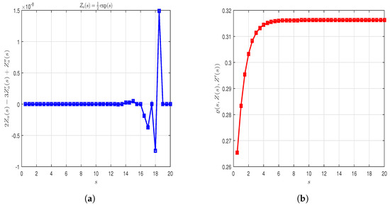
Consider the linear differential equation,

$$2Z\left(s\right)-3Z^{\prime }\left(s\right)+Z^{″}\left(s\right)=\frac{1}{\sqrt{10}+e^{-s}},$$

(29)

with initial conditions $Z\left(0\right)=Z_0=\frac{1}{3}$, $Z^{\prime }\left(0\right)=Z_1=\frac{11}{9}$. We can assert that ${\gamma }_0=2$, ${\gamma }_1=-3$, and

$$\varrho (s,Z\left(s\right),Z^{\prime }\left(s\right))=\frac{1}{\sqrt{10}+e^{-s}}.$$

For $\epsilon =\frac{1}{3}$, it is straightforward to verify that the function $Z_a\left(s\right)=\frac{1}{2}{e}^s$ satisfies

$$\left|2Z\left(s\right)-3Z^{\prime }\left(s\right)+Z^{″}\left(s\right)-\frac{1}{\sqrt{10}+e^{-s}}\right|\le \frac{1}{3},$$

(30)

for each $s>0$, and by employing initial values, we obtain an exact solution to (29):

$$\begin{array}{cc}\hfill Z\left(s\right)& =-{\mathrm{e}}^{2s}\left(e^{-s}-\sqrt{10}ln\left(e^s+\frac{\sqrt{10}}{10}\right)+\sqrt{10}s\right)\hfill \\ \hfill & -e^s\left(ln\left(\frac{\sqrt{10}}{10}+1\right)+\sqrt{10}-\frac{10(1+\sqrt{10})}{\sqrt{10}+10}+\frac{5}{9}\right)\hfill \\ \hfill & -e^{2s}\left(\sqrt{10}ln\left(\frac{\sqrt{10}}{10}+1\right)-\sqrt{10}+\frac{10(1+\sqrt{10})}{\sqrt{10}+10}-\frac{17}{9}\right)\hfill \\ \hfill & -e^s\left(s-ln\left({\mathrm{e}}^s+\frac{\sqrt{10}}{10}\right)\right).\hfill \end{array}$$

(31)

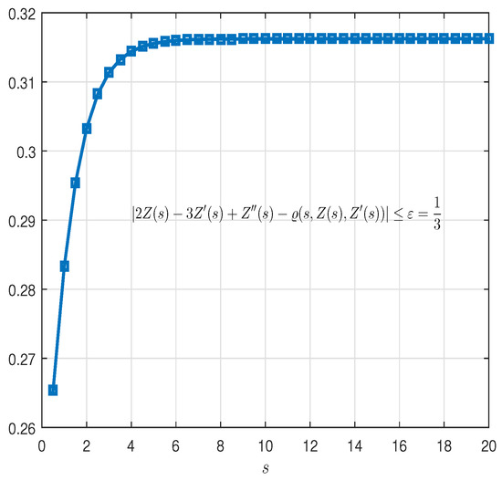
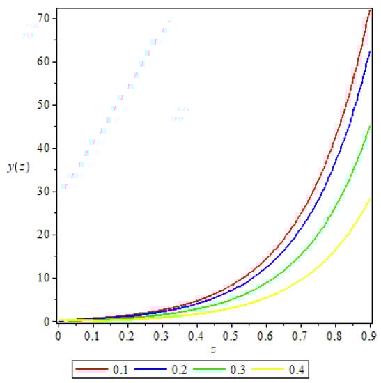
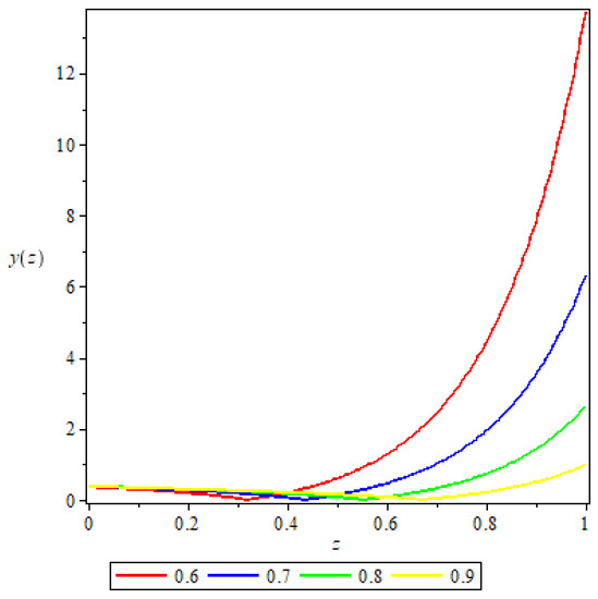
One can see these results in Table 2, and in the graphical representation of $2Z_a\left(s\right)-3Z_a^{\prime }\left(s\right)+Z_a^{″}\left(s\right)$ whenever $Z_a\left(s\right)=\frac{1}{2}{e}^s$, $\varrho (s,Z\left(s\right),Z^{\prime }\left(s\right))$, and Inequality (30) for $s>0$, in Figure 1a,b and Figure 2, respectively; therefore, all the conditions of Theorem 3 are satisfied, and (29) has HUS in class Ψ.

Table 2. Numerical results of $Z_a\left(s\right)$, $\varrho (s,Z\left(s\right),Z^{\prime }\left(s\right))$, and Inequality (30) for $s>0$ in Example 1.

s	${\mathit{Z}}_{\mathit{a}}\left(\mathit{s}\right)$	$\mathit{\varrho }(\mathit{s},\mathit{Z}\left(\mathit{s}\right),{\mathit{Z}}^{\prime }\left(\mathit{s}\right))$	Ineq. (30)	Exact Solution
$0.50$	$0.82436$	$0.26534$	$0.26534$	$1.5525$
$1.00$	$1.35914$	$0.28327$	$0.28327$	$5.4320$
$1.50$	$2.24085$	$0.29539$	$0.29539$	$16.9203$
$2.00$	$3.69453$	$0.30325$	$0.30325$	$49.7102$
$2.50$	$6.09125$	$0.30823$	$0.30823$	$141.4213$
$3.00$	$10.04277$	$0.31133$	$0.31133$	$394.9732$
$3.50$	$16.55773$	$0.31324$	$0.31324$	$1091.2161$
$4.00$	$27.29908$	$0.31441$	$0.31441$	$2995.3715$
$4.50$	$45.00857$	$0.31512$	$0.31512$	$8190.4806$
$5.00$	$74.20658$	$0.31556$	$0.31556$	22,343.7060
$5.50$	$122.34597$	$0.31582$	$0.31582$	60,868.0217
$6.00$	$201.71440$	$0.31598$	$0.31598$	165,673.4726
$6.50$	$332.57082$	$0.31608$	$0.31608$	450,705.1967
$7.00$	$548.31658$	$0.31614$	$0.31614$	1,225,734.1757
$7.50$	$904.02121$	$0.31617$	$0.31617$	3,332,864.5664
$8.00$	$1490.47899$	$0.31619$	$0.31619$	9,061,270.6082
$8.50$	$2457.38442$	$0.31621$	$0.31621$	24,633,734.3046
$9.00$	$4051.54196$	$0.31622$	$0.31622$	66,965,796.7799
$9.50$	$6679.86342$	$0.31622$	$0.31622$	182,039,104.4573
$10.00$	11,013.23290	$0.31622$	$0.31622$	494,845,453.9945
⋮	⋮	⋮	⋮	⋮

Figure 1. 2D plot of $2Z_a\left(s\right)-3Z_a^{\prime }\left(s\right)+Z_a^{″}\left(s\right)$, whenever $Z_a\left(s\right)=\frac{1}{2}{e}^s$, $\varrho (s,Z\left(s\right),Z^{\prime }\left(s\right))$, and Inequality (30) for $s>0$ in Example 1; (a) $2Z_a\left(s\right)-3Z_a^{\prime }\left(s\right)+Z_a^{″}\left(s\right)$; (b) $\varrho (s,Z\left(s\right),Z^{\prime }\left(s\right))$.

Figure 2. 2D plot of Inequality (30) for $s>0$ in Example 1.

6.2. Stability of Nonlinear Differential Equation

Example 2.

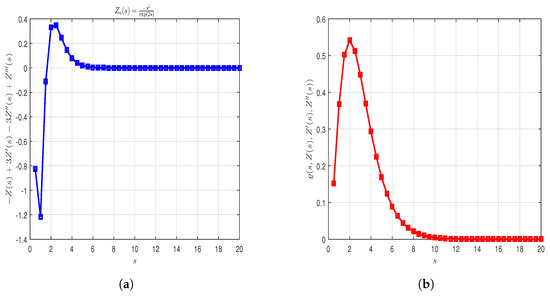
Consider the nonlinear differential equation,

$$-Z\left(s\right)+3Z^{\prime }\left(s\right)-3Z^{\prime \prime }\left(s\right)+Z^{\prime \prime \prime }\left(s\right)=\frac{s^2}{e^{-s}},$$

(32)

with initial conditions $Z\left(0\right)=Z_0=\frac{2}{5}$, $Z^{\prime }\left(0\right)=Z_1=\frac{1}{7}$, and $Z^{″}\left(0\right)=Z_2=\frac{-3}{2}$. We can assert that ${\gamma }_0=-1$, ${\gamma }_1=3$, ${\gamma }_2=-3$, and

$$\varrho (s,Z\left(s\right),Z^{\prime }\left(s\right),Z^{″}\left(s\right))=\frac{s^2}{e^{-s}}.$$

For $\epsilon =\frac{1}{5}$, it is straightforward to verify that the function $Z_a\left(s\right)=\frac{-s^2}{e^{2s}}$ satisfies

$$\left|-Z\left(s\right)+3Z^{\prime }\left(s\right)-3Z^{″}\left(s\right)+Z^{‴}\left(s\right)-\frac{s^2}{e^{-s}}\right|\le \frac{1}{5}\varphi \left(s\right),$$

(33)

for each $s>0$ where $\varphi \left(s\right)=99,999s^4$, and by employing initial values, we obtain an exact solution to (29):

$$\begin{array}{cc}\hfill Z\left(s\right)& =\frac{31e^s}{40}-\frac{159s^2{e}^s}{280}-\frac{e^{-s}\left(16s^4+32s^3+48s^2+48s+24\right)}{64}\hfill \\ \hfill & -\frac{177s{e}^s}{280}+\frac{s{e}^{-s}\left(8s^3+12s^2+12s+6\right)}{16}-\frac{s^2{e}^{-s}\left(4s^2+4s+2\right)}{16}.\hfill \end{array}$$

(34)

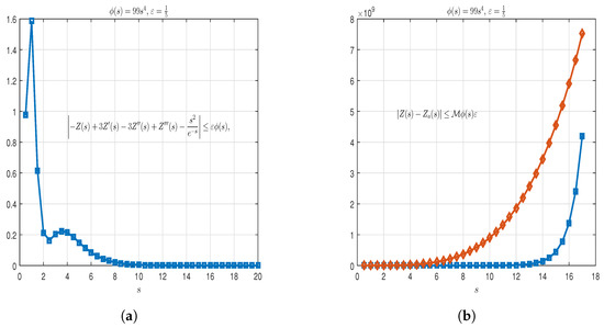
One can see these results in Table 3, and in the graphical representation of

$$-Z\left(s\right)+3Z^{\prime }\left(s\right)-3Z^{\prime \prime }\left(s\right)+Z^{\prime \prime \prime }\left(s\right),$$

whenever $Z_a\left(s\right)=\frac{-s^2}{e^{2s}}$, $\varrho (s,Z\left(s\right),Z^{\prime }\left(s\right),Z^{″}\left(s\right))$, Inequality (33), and $\left|Z\left(s\right)-Z_a\left(s\right)\right|$, for $s>0$ in Figure 3a,b and Figure 4a,b, respectively. Therefore, all the conditions of Theorem 7 are satisfied. Hence, (32) has HUS in the class Ψ.

Table 3. Numerical results of $Z_a\left(s\right)$, $\varrho (s,Z\left(s\right),Z^{\prime }\left(s\right),Z^{″}\left(s\right))$, Inequality (33), and $\left|Z\left(s\right)-Z_a\left(s\right)\right|$, $\mathcal{M}\varphi \left(s\right)\epsilon$ for $s>0$ in Example 2.

s	${\mathit{Z}}_{\mathit{a}}\left(\mathit{s}\right)$	$\mathit{\varrho }(\mathit{s},\mathit{Z}\left(\mathit{s}\right),{\mathit{Z}}^{\prime }\left(\mathit{s}\right))$	Ineq. (30)	Exact Solution	$\left|\mathit{Z}\left(\mathit{s}\right)-{\mathit{Z}}_{\mathit{a}}\left(\mathit{s}\right)\right|$	$\mathcal{M}\mathit{\varphi }\left(\mathit{s}\right)\mathit{\epsilon }$
$0.50$	$-0.09197$	$0.15163$	$0.97936$	$0.1625$	$0.2544$	$5624.9438$
$1.00$	$-0.13534$	$0.36788$	$1.58590$	$-1.4772$	$1.3418$	$\mathrm{89,999.1000}$
$1.50$	$-0.11202$	$0.50204$	$0.61406$	$-6.7744$	$6.6624$	$\mathrm{455,620.4438}$
$2.00$	$-0.07326$	$0.54134$	$0.21166$	$-20.6190$	$20.5457$	$\mathrm{1,439,985.6000}$
$2.50$	$-0.04211$	$0.51303$	$0.16434$	$-53.2201$	$53.1780$	$\mathrm{3,515,589.8438}$
$3.00$	$-0.02231$	$0.44808$	$0.20269$	$-125.3066$	$125.2843$	$\mathrm{7,289,927.1000}$
$3.50$	$-0.01117$	$0.36992$	$0.22425$	$-278.0600$	$278.0489$	$\mathrm{13,505,489.9438}$
$4.00$	$-0.00537$	$0.29305$	$0.21455$	$-591.8759$	$591.8706$	$\mathrm{23,039,769.6000}$
$4.50$	$-0.00250$	$0.22496$	$0.18525$	$-1221.4710$	$1221.4685$	$\mathrm{36,905,255.9438}$
$5.00$	$-0.00114$	$0.16845$	$0.14925$	$-2461.0444$	$2461.0433$	$\mathrm{56,249,437.5000}$
$5.50$	$-0.00051$	$0.12363$	$0.11464$	$-4864.3699$	$4864.3694$	$\mathrm{82,354,801.4438}$
$6.00$	$-0.00022$	$0.08924$	$0.08514$	$-9464.7453$	$9464.7451$	$\mathrm{116,638,833.6000}$
$6.50$	$-0.00010$	$0.06352$	$0.06170$	$-\mathrm{18,175.6012}$	$\mathrm{18,175.6011}$	$\mathrm{160,654,018.4438}$
$7.00$	$-0.00004$	$0.04468$	$0.04388$	$-\mathrm{34,516.5370}$	$\mathrm{34,516.5369}$	$\mathrm{216,087,839.1000}$
$7.50$	$-0.00002$	$0.03111$	$0.03077$	$-\mathrm{64,923.2572}$	$\mathrm{64,923.2572}$	$\mathrm{284,762,777.3438}$
$8.00$	$-0.00001$	$0.02147$	$0.02132$	$-\mathrm{121,101.4220}$	$\mathrm{121,101.4220}$	$\mathrm{368,636,313.6000}$
$8.50$	$0.00000$	$0.01470$	$0.01464$	$-\mathrm{224,240.7191}$	$\mathrm{224,240.7191}$	$\mathrm{469,800,926.9438}$
$9.00$	$0.00000$	$0.01000$	$0.00997$	$-\mathrm{412,533.7924}$	$\mathrm{412,533.7924}$	$\mathrm{590,484,095.1000}$
$9.50$	$0.00000$	$0.00676$	$0.00674$	$-\mathrm{754,550.2155}$	$\mathrm{754,550.2155}$	$\mathrm{733,048,294.4438}$
$10.00$	$0.00000$	$0.00454$	$0.00454$	$-\mathrm{1,372,956.8133}$	$\mathrm{1,372,956.8133}$	$\mathrm{899,991,000.0000}$
⋮	⋮	⋮	⋮	⋮	⋮	⋮

Figure 3. 2D plot of $2Z_a\left(s\right)-3Z_a^{\prime }\left(s\right)+Z_a^{″}\left(s\right)$ whenever $Z_a\left(s\right)=\frac{-s^2}{e^{2s}}$ and $\varrho (s,Z\left(s\right),Z^{\prime }\left(s\right))$ for $s>0$ in Example 2; (a) $-Z\left(s\right)+3Z^{\prime }\left(s\right)-3Z^{\prime \prime }\left(s\right)+Z^{\prime \prime \prime }\left(s\right)$; (b) $\varrho (s,Z\left(s\right),Z^{\prime }\left(s\right),Z^{\prime \prime }\left(s\right))$.

Figure 4. 2D plot of Inequality (33) and $\left|Z\left(s\right)-Z_a\left(s\right)\right|\le \varphi \left(s\right)\epsilon$ for $s>0$ in Example 2; (a) Inequality (33); (b) $\left|Z\left(s\right)-Z_a\left(s\right)\right|\le \mathcal{M}\varphi \left(s\right)\epsilon$.

6.3. Stability of Fractional Differential Equation

In this section, we look at a few fractional differential equation applications of the Tarig transform technique.

We take into account the following general fractional-order linear differential equation:

$${}^c{D}_{0^{+}}^{\mu }\left(\mathfrak{z}\right)=\sum _{\ell =0}^{\phi }{e}_{\ell }{y}^{\left(\ell \right)}\left(\mathfrak{z}\right)+\xi \left(\mathfrak{z}\right),\phi -1<\mu \le \phi ,$$

(35)

subject to the initial condition,

$$y^{\left(\ell \right)}\left(0\right)=c_{\ell },i=0,\dots ,\phi -1,c_{\ell },e_j\in R.$$

(36)

Through the Tarig transform of (35), we obtain

$$\mathsf{{\rm Y}}{(}^c{D}_{0^{+}}^{\mu }\left(\mathfrak{z}\right))=\mathsf{{\rm Y}}\left(\sum _{\ell =0}^{\phi }{e}_{\ell }{y}^{\left(\ell \right)}\left(\mathfrak{z}\right)+\xi \left(\mathfrak{z}\right)\right),\phi -1<\mu \le \phi .$$

Using the linearity of the Tarig transform, we obtain

$$\begin{array}{cc}\hfill \mathsf{{\rm Y}}{(}^c{D}_{0^{+}}^{\mu }\left(\mathfrak{z}\right))& =\mathsf{{\rm Y}}\left(\sum _{\ell =0}^{\phi }{e}_{\ell }{y}^{\left(\ell \right)}\left(\mathfrak{z}\right)\right)+\mathsf{{\rm Y}}\left(\xi \left(\mathfrak{z}\right)\right),\phi -1<\mu \le \phi \hfill \\ \hfill & =e_{0}y\left(\mathfrak{z}\right)+\sum _{\ell =1}^{\phi }{e}_{\ell }\mathsf{{\rm Y}}\left(y^{\left(\ell \right)}\left(\mathfrak{z}\right)\right)+\mathsf{{\rm Y}}\left(\xi \left(\mathfrak{z}\right)\right).\hfill \end{array}$$

Applying the Tarig transform to the derivatives, we obtain

$$\begin{array}{cc}\hfill {\left(\frac{\varphi }{v}\right)}^{\mu }\mathsf{Ḩ}(v,\varphi )-\sum _{k=0}^{\phi -1}{\left(\frac{\varphi }{v}\right)}^{k+1-\mu }{y}^{\left(k\right)}\left(0\right)& =e_0\mathsf{Ḩ}(v,\varphi )+\sum _{\ell =1}^{\phi }{e}_{\ell }\left[{\left(\frac{\varphi }{v}\right)}^{-\ell }\mathsf{Ḩ}(v,\varphi )-\sum _{k=0}^{\ell -1}{\left(\frac{\varphi }{v}\right)}^{k+1-\ell }{y}^{\left(k\right)}\left(0\right)\right]+\mathsf{{\rm Y}}\left(\xi \left(\mathfrak{z}\right)\right)\hfill \\ \hfill {\left(\frac{\varphi }{v}\right)}^{\mu }\mathsf{Ḩ}(v,\varphi )-\sum _{\ell =0}^{\phi -1}{e}_{\ell }{\left(\frac{\varphi }{v}\right)}^{-\ell }\mathsf{Ḩ}(v,\varphi )& =\sum _{k=0}^{\phi -1}{c}_k{\left(\frac{\varphi }{v}\right)}^{k+1-\mu }-\sum _{\ell =1}^{\phi }{e}_{\ell }\sum _{k=0}^{\ell -1}{c}_k{\left(\frac{\varphi }{v}\right)}^{k+1-\ell }+\mathsf{{\rm Y}}\left(\xi \left(\mathfrak{z}\right)\right)\hfill \end{array}$$

$$\begin{array}{cc}\hfill \mathsf{Ḩ}(v,\varphi )& ={\left({\left(\frac{\varphi }{v}\right)}^{\mu }-\sum _{\ell =0}^{\phi -1}{e}_{\ell }{\left(\frac{\varphi }{v}\right)}^{-\ell }\right)}^{-1}\left(\sum _{k=0}^{\phi -1}{c}_k{\left(\frac{\varphi }{v}\right)}^{k+1-\mu }-\sum _{\ell =1}^{\phi }{e}_{\ell }\sum _{k=0}^{\ell -1}{c}_k{\left(\frac{\varphi }{v}\right)}^{k+1-\ell }+\mathsf{{\rm Y}}\left(\xi \left(\mathfrak{z}\right)\right)\right).\hfill \end{array}$$

(37)

Applying the inverse Tarig transform to both sides of Equation (37) yields the solution to Equation (35):

$$\begin{array}{cc}\hfill y\left(\mathfrak{z}\right)& ={\mathsf{{\rm Y}}}^{-1}\left[{\left({\left(\frac{\varphi }{v}\right)}^{\mu }-\sum _{\ell =0}^{\phi -1}{e}_{\ell }{\left(\frac{\varphi }{v}\right)}^{-\ell }\right)}^{-1}\left(\sum _{k=0}^{\phi -1}{c}_k{\left(\frac{\varphi }{v}\right)}^{k+1-\mu }-\sum _{\ell =1}^{\phi }{e}_{\ell }\sum _{k=0}^{\ell -1}{c}_k{\left(\frac{\varphi }{v}\right)}^{k+1-\ell }+\mathsf{{\rm Y}}\left(\xi \left(\mathfrak{z}\right)\right)\right)\right].\hfill \\ \hfill \end{array}$$

(38)

Remark 1.

If $n=1,e_0=-1$ and $e_1=\xi \left(\mathfrak{z}\right)=0$, then

$${}^c{D}^{\mu }y\left(\mathfrak{z}\right)+y\left(\mathfrak{z}\right)=0,0<\mu \le 1,\mathfrak{z}>0$$

(39)

with initial condition

$$y\left(0\right)=1.$$

(40)

Substituting $\phi ,e_0,e_1$ and ξ in (38), we obtain

$$\begin{array}{cc}\hfill y\left(\mathfrak{z}\right)& ={\mathsf{{\rm Y}}}^{-1}\left[{\left({\left(\frac{\varphi }{v}\right)}^{-\mu }-\sum _{\ell =0}^{\phi -1}{e}_{\ell }{\left(\frac{\varphi }{v}\right)}^{-\ell }\right)}^{-1}{\left(\frac{\varphi }{v}\right)}^{1-\mu }\right]\hfill \\ \hfill & ={\mathsf{{\rm Y}}}^{-1}\left[\left(\frac{\varphi }{v}\right)-{\left(1-(-1)\left(\frac{\varphi }{v}\right)\right)}^{-1}\right]\hfill \end{array}$$

and

$$\mathsf{Ḩ}(v,\varphi )=\mathsf{{\rm Y}}\left(E_{\mu }(-{\mathfrak{z}}^{\mu })\right).$$

(41)

Through the inverse Tarig transform of (41), we obtain the exact solution to Equation (39), as follows:

$$y\left(\mathfrak{z}\right)=E_{\mu }(-{\mathfrak{z}}^{\mu }).$$

(42)

Figure 5 and Figure 6 show the two-dimensional surfaces of the exact solution (42) of the differential Equation (35), as well as its graphical results, with regard to μ.

Figure 5. Solution curve $y\left(\mathfrak{z}\right)$ for $\mu =0.1,0.2,0.3,0.4$.

Figure 6. Solution curve $y\left(\mathfrak{z}\right)$ for $\mu =0.6,0.7,0.8,0.9$.

7. Conclusions

This manuscript has discussed the Tarig transform for non-homogeneous and homogeneous linear differential equations. Using this unique integral transform, we resolved higher-order linear differential equations, and we produced the conditions required for HUS, by using the Tarig transform to show that a linear differential equation was stable. This study also demonstrated that the Tarig transform method is more effective for analyzing the stability issue for differential equations with constant coefficients. A discussion of applications followed, to illustrate our approach. Moreover, this paper proposes a new method of investigating the HUS of differential equations. In the future, we will investigate the stability of fractional differential equations.

References

- Debnath, L.; Bhatta, D.D. Integral Transforms and Their Applications, 2nd ed.; Chapman & Hall/CRC: Boca Raton, FL, USA, 2007. [Google Scholar]
- Kılıçman, A.; Gadain, H.E. An application of double Laplace transform and double Sumudu transform. Lobachevskii J. Math. 2009, 30, 214–223. [Google Scholar] [CrossRef]
- Zhang, J. A Sumudu based algorithm for solving differential equations. Comput. Sci. J. Moldova 2007, 15, 303–313. [Google Scholar]
- Eltayeb, H.; Kılıçman, A. A note on the Sumudu transforms and differential equations. Appl. Math. Sci. (Ruse) 2010, 4, 1089–1098. [Google Scholar]
- Kılıçman, A.; Eltayeb, H. A note on integral transforms and partial differential equations. Appl. Math. Sci. (Ruse) 2010, 4, 109–118. [Google Scholar]
- Eltayeb, H.; Kılıçman, A. On some applications of a new integral transform. Int. J. Math. Anal. (Ruse) 2010, 4, 123–132. [Google Scholar]
- Manjarekar, S.; Bhadane, A.P. Applications of Tarig transformation to new fractional derivatives with non singular kernel. J. Fract. Calc. Appl. 2018, 9, 160–166. [Google Scholar]
- Loonker, D.; Banerji, P.K. Fractional Tarig transform and Mittag-Leffler function. Bol. Soc. Parana. Mat. 2017, 35, 83–92. [Google Scholar] [CrossRef]
- Elzaki, T.M.; Elzaki, S.M. On the relationship between Laplace transform and new integral transform “Tarig Transform”. Elixir Appl. Math. 2011, 36, 3230–3233. [Google Scholar]
- Elzaki, T.M.; Elzaki, S.M. On the Connections Between Laplace and Elzaki transforms. Adv. Theor. Appl. Math. 2011, 6, 1–11. [Google Scholar]
- Obłoza, M. Hyers stability of the linear differential equation. Rocznik Nauk.-Dydakt. Prace Mat. 1993, 13, 259–270. [Google Scholar]
- Obłoza, M. Connections between Hyers and Lyapunov stability of the ordinary differential equations. Rocznik Nauk.-Dydakt. Prace Mat. 1997, 14, 141–146. [Google Scholar]
- Alsina, C.; Ger, R. On some inequalities and stability results related to the exponential function. J. Inequal. Appl. 1998, 2, 373–380. [Google Scholar] [CrossRef]
- Huang, J.; Li, Y.J. Hyers-Ulam stability of linear functional differential equations. J. Math. Anal. Appl. 2015, 426, 1192–1200. [Google Scholar]
- Zada, A.; Shah, S.O.; Shah, R. Hyers-Ulam stability of non-autonomous systems in terms of boundedness of Cauchy problems. Appl. Math. Comput. 2015, 271, 512–518. [Google Scholar] [CrossRef]
- Choi, G.; Jung, S.-M. Invariance of Hyers-Ulam stability of linear differential equations and its applications. Adv. Differ. Equ. 2015, 2015, 277. [Google Scholar] [CrossRef]
- Hyers, D.H. On the stability of the linear functional equation. Proc. Natl. Acad. Sci. USA 1941, 27, 222–224. [Google Scholar] [CrossRef]
- Jung, S.-M. Hyers-Ulam stability of linear differential equations of first order. Appl. Math. Lett. 2004, 17, 1135–1140. [Google Scholar] [CrossRef]
- Jung, S.-M. Hyers-Ulam stability of linear differential equations of first order. III. J. Math. Anal. Appl. 2005, 311, 139–146. [Google Scholar] [CrossRef]
- Jung, S.-M. Hyers-Ulam stability of linear differential equations of first order. II. Appl. Math. Lett. 2006, 19, 854–858. [Google Scholar] [CrossRef]
- Li, Y.J.; Shen, Y. Hyers-Ulam stability of nonhomogeneous linear differential equations of second order. Int. J. Math. Math. Sci. 2009, 2009, 576852. [Google Scholar] [CrossRef]
- Li, Y.J.; Shen, Y. Hyers-Ulam stability of linear differential equations of second order. Appl. Math. Lett. 2010, 23, 306–309. [Google Scholar] [CrossRef]
- Miura, T.; Miyajima, S.; Takahasi, S.-E. A characterization of Hyers-Ulam stability of first order linear differential operators. J. Math. Anal. Appl. 2003, 286, 136–146. [Google Scholar] [CrossRef]
- Ulam, S.M. A Collection of Mathematical Problems; Interscience Tracts in Pure and Applied Mathematics, no. 8; Interscience Publishers: New York, NY, USA, 1960. [Google Scholar]
- Wang, G.W.; Zhou, M.R.; Sun, L. Hyers-Ulam stability of linear differential equations of first order. Appl. Math. Lett. 2008, 21, 1024–1028. [Google Scholar] [CrossRef]
Disclaimer/Publisher’s Note: The statements, opinions and data contained in all publications are solely those of the individual author(s) and contributor(s) and not of MDPI and/or the editor(s). MDPI and/or the editor(s) disclaim responsibility for any injury to people or property resulting from any ideas, methods, instructions or products referred to in the content. |
© 2023 by the authors. Licensee MDPI, Basel, Switzerland. This article is an open access article distributed under the terms and conditions of the Creative Commons Attribution (CC BY) license (https://creativecommons.org/licenses/by/4.0/).