Abstract
This paper presents mathematical models to estimate the kinematics and dynamics of wheeled and tracked robots. The models account for the physical–mechanical characteristics of the ground, the influence of the center of gravity displacement on the cornering moment of resistance, and the influence of the interaction of the crawler with the roadway. The results of the models are characterized by defining computational relationships for a robot’s equations of motion, longitudinal forces, transverse forces, and resistive turning moments generated via longitudinal forces and transverse forces.
MSC:
37M05
1. Introduction
The design, construction, experimentation, and functional analysis of wheeled or tracked robots have experienced exponential development over the past 30 years [1,2]; consequently, scientific articles, books, and conference papers have also experienced a veritable explosion, resulting in an immense amount of scientific and technical information concerning the kinematics and dynamics of robots. In specialized works, the kinematics and dynamics of robots are addressed according to the type of robot, which are classified based on two criteria: (1) the type of propulsion, i.e., with wheels [3,4,5], with tracks [6], or with legs [7,8]; (2) the mass of the robot, i.e., light or heavy.
Wheeled robots have widespread applications due to a wide range of advantages, including constructive simplicity, versatility in the layout of the motor-reducer, very high versatility allowing for the configuration of the propulsion in accordance with the specific application, and various possibilities for individual and group control of the wheels.
The structure of the wheel drive is built from a rational technical compromise of the following: moving in a straight direction on terrain with an imposed microgeometry, crossing obstacles, executing a turn (moving on a curvilinear trajectory), and ensuring stability during movement.
Depending on the vertical displacement capacity of the plane containing the wheel axis, the following types of constructive solutions are found for wheeled propulsion systems [1]:
- Propulsion systems where the horizontal plane, which contains the wheel axis, cannot move vertically because, from a physical point of view, the wheel is mounted on the fixed axis of the gearmotor; it is the most often used solution for small-sized wheeled robots intended to move relatively short distances, most often via real-time human control, which allows for avoiding critical situations; from a constructive point of view, the solution is simple, robust, and leads to lower costs; the gearmotor can be arranged by fixing on the platform, or it can be arranged in the wheel.
- Propulsion systems where the horizontal plane, which contains the wheel axis, can move vertically for very short distances (maximum equal to the wheel radius); this is the case for the propulsion systems where the wheels are provided with individual suspension for each wheel to improve the stability of the platform; this is the solution used for medium and large robots intended to move over medium and long distances autonomously on steep terrain.
- Propulsion systems where the horizontal plane, which contains the wheel axis, can move vertically for large distances; these structures have individually articulated wheels at the extremities of planar structures comprised of articulated bars that can be controlled independently (legs).
Depending on the relative position in the space of the wheel centers, there are wheel drive solutions in which the wheel center position is kept constant. These wheel drive solutions have variations within the functional limits of the suspensions or structures in which the wheel center position changes substantially, allowing for the exploitation of the advantage offered in the possibility of changing the turning radius only when traveling at low speeds, which would provide time for the modification of the structure and the use of appropriate systems to change the configuration under conditions where the wheels are in contact with the ground [9,10].
Depending on the number of wheels; the role of the wheels in the movement of the robot; driving, free, or directional wheels; and the execution of the turn via turning or skid steering, the following wheeled thrusters are distinguished: two-wheel propulsion systems [11,12], three-wheel propulsion systems, or four-wheel propulsion systems [13,14].
Four-wheel propulsion systems ensure superior stability in turns and a more favorable distribution of a robot’s weight. As a rule, the wheel centers are grouped two by two to be located in the corners of a rectangle. In the case of robots with the axes of all fixed wheels, the turn is performed by changing the speed of the wheels on one side in relation to the speed of the wheels located on the opposite side (the turn is performed by skidding off the wheels, i.e., skid steering). When the axes of the two wheels coincide, and the respective wheels keep their plane of symmetry, and at the same time, the planes of the other wheels can rotate, the turn is executed by turning the wheels.
Tracked robots are used in multiple military applications or actions with a high degree of danger due to their increased ability to move in an unstructured environment (rough, off-road terrain) but also due to the increased ability of the propulsion system to tackle complex obstacles with a positive contribution to mobility. The vast majority of tracked robots have a structure consisting only of two tracks arranged on one side and the other of the chassis (platform). In the case of tracked robots, the propulsion system is a component of the running system that also includes the suspension system [15]. The main advantages of tracked robots are the simplicity of actuation and control using two electric motors, high maneuverability and wide range of turning radii, low average ground pressure which allows for good mobility on soft soils, high load capacity, high stability, and constructive compactness. The major disadvantages of this type of propulsion are complicated track and drive wheel construction, low efficiency, need for higher drive power, and higher dead weight compared to a wheeled robot.
The novel aspect of our research concerns the exhaustive exemplification of kinematic and dynamic models for wheeled and tracked robotic vehicles. This research has the advantage of presenting in a single, succinct material the advantages and disadvantages of the two propulsion systems. When designing a ground robot and knowing locally where it needs to intervene, the highlighted patterns help to easily identify the best solution. Analytical models are simple and allow for loading them into robot controllers [16,17]. These models allow for the identification of disturbances that occur when making turns. Also, the data coming from navigation sensors can be immediately associated.
This paper is structured as follows: Section 2 presents the general aspects of the kinematics and dynamics of wheeled and tracked Unmanned Ground Vehicles (UGVs); Section 3 presents the study on the kinematics and dynamics of two- and four-wheel drive/directional UGVs; Section 4 describes how four-wheeled UGVs behave when turning and their behavior during skids; Section 5 describes the kinematics and dynamics of tracked UGVs; Section 6 presents the conclusions and potential for further development.
2. Aspects Regarding the Kinematics and Dynamics of Wheeled and Tracked UGVs
Kinematics aims to determine the trajectory on which the robot moves depending on the position of the planes of the guide wheels and the angular velocities of the wheels.
In the case of direct kinematics, the values of the angular velocities of the wheels, their disposition, and the position of the symmetry planes of the steering wheels, as well as the moments applied to the driving wheels, are considered to be known, and the purpose is determining the robot’s trajectory.
In the case of inverse kinematics, the trajectory on which the robot must move is imposed, and the values of the kinematic parameters that allow this are determined.
The absence of slips is considered in the longitudinal plane. In the transverse plane, there may be slips due to the following functional aspects:
- The positioning of the steering wheel planes does not rigorously respect the calculation relationship that conditions the absence of lateral slips;
- Elasticity in the transverse direction of the tires used in the construction of the wheels;
- Executing the turn via skidding (skid steering).
The execution of the turn frequently intervenes in the movement of the robots, aiming to follow the trajectory of the imposed curve, avoid the obstacle, and correct the movement trajectory to minimize the deviations from the imposed trajectory and change the displacement trajectory as a result of the reconfiguration of the imposed trajectory.
In the case of rigid platforms with wheels that do not change their position on the plane of symmetry, the turn is executed only via the method of introducing speed differences for the left-right wheels; this method of executing the turn involves the significant lateral sliding of the wheels, which is known as skid steering [18].
Regarding the propulsion systems where the turn is performed by rotating the plane of symmetry of the wheels, the more frequently used solutions are distinguished in Figure 1a,b [19].
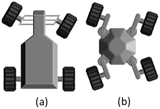
Figure 1.
(a) Ackermann-type steering system; (b) independent wheel steering [19].
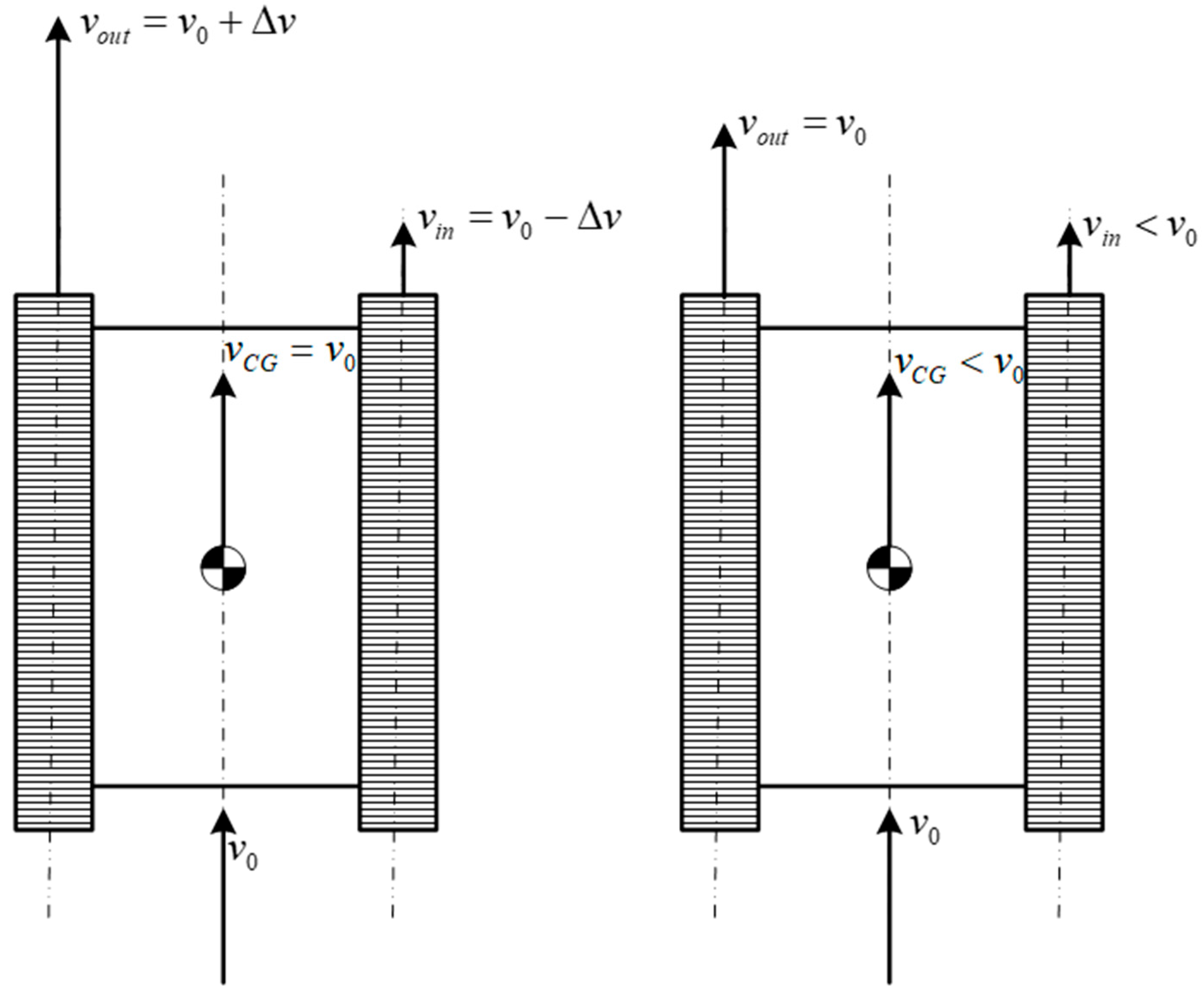
In the case of tracked platforms, the turn is performed by skidding, i.e., by rotating the two tracks at different angular speeds. The following situations can be distinguished (Figure 2) [20]:
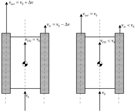
Figure 2.
The turning of tracked robots [20].
- The track that is on the outside of the turn will have a speed Δv higher than the speed at which the platform was traveling before entering the turn, while the track located toward the center of the turn will have a speed lower than the speed of the lower outer track with Δv compared to the speed with which the platform was moving before entering the turn;
- The track on the outside of the turn maintains its speed unchanged, while a track on the inside of the turn decreases its speed, possibly reaching zero.
The execution of the turn via skidding is characterized by the following essential aspects:
- The wheels keep their plane of symmetry unchanged;
- The turning radius depends on the speeds of the wheels on the two sides of the robot;
- The turning process is accompanied by the lateral slipping of the wheels.
A disadvantage of this method of turning is the significant energy consumption required to compensate for the friction generated in the wheel/track skidding process, as well as the control difficulties due to longitudinal slips. The existence of intense wheel-ground relative slips also causes the accelerated wear of the wheel/track contact surface [21,22,23], especially for heavy robots.
In the case of wheeled robots that perform a turn by turning the steering wheels, the trajectory characteristics depend only on the dimensions and structure of the propulsion system and have a weak correlation with the dynamic model, assuming pure rolling of the wheels (no longitudinal/lateral slips).
In contrast to the above situation, in the case of robots performing a skid turn, there is a close correlation between the kinematic model and the dynamic model of the propulsion system. Thus, it is necessary to determine from the dynamic model the forces and moments acting on the wheels/tracks to estimate the longitudinal and lateral slips based on them to determine the characteristics of the robot’s trajectory [24]. The forces and moments that appear in the turn depend, among other factors, on the kinematic characteristics of the movement (speed, turning radius, propulsion dimensions, etc.).
Next, considering the works from the analyzed specialized literature, applied kinematic and dynamic models for wheeled and tracked robots are presented. As demonstrated in [25,26,27], tracked vehicles with power steering are well received via UGV configurations. The analytical models used allow for obtaining a high degree of prediction regarding traversability. Also, the concepts of mobility and stability for non-cohesive terrains can be generalized, with applicability, including for UGVs on wheels.
The authors of [28,29,30] demonstrate the need to achieve very precise control of land robots on wheels and tracks. The control laws and the adaptive and predictive control algorithms must lead to values close to the experimentally obtained values with maximum errors of 2–3% [31,32,33,34]. The kinematic and dynamic representations must allow for the estimation of sideslip angles without increasing the noise level.
By going through the models in [35,36,37,38,39,40,41], it was found that the consideration of slip effects is especially useful, as it does not introduce complexity from dynamic calculations in the loop. The best way to obtain results is a combined method starting from experimental results to form the basis of an optimized kinematic model for tracked and wheeled UGVs, which accounts for the instantaneous centers of rotation (ICR).
Kinematic models focus on the presentation of assumptions, calculation schemes, and main constitutive equations. Dynamic models focus on determining the forces and moments acting on the wheels and the robot and determining the influences that longitudinal and transverse slips have on the travel trajectory.
3. Kinematics and Dynamics Study of Four-Wheeled Robots with Two-Directional Wheels
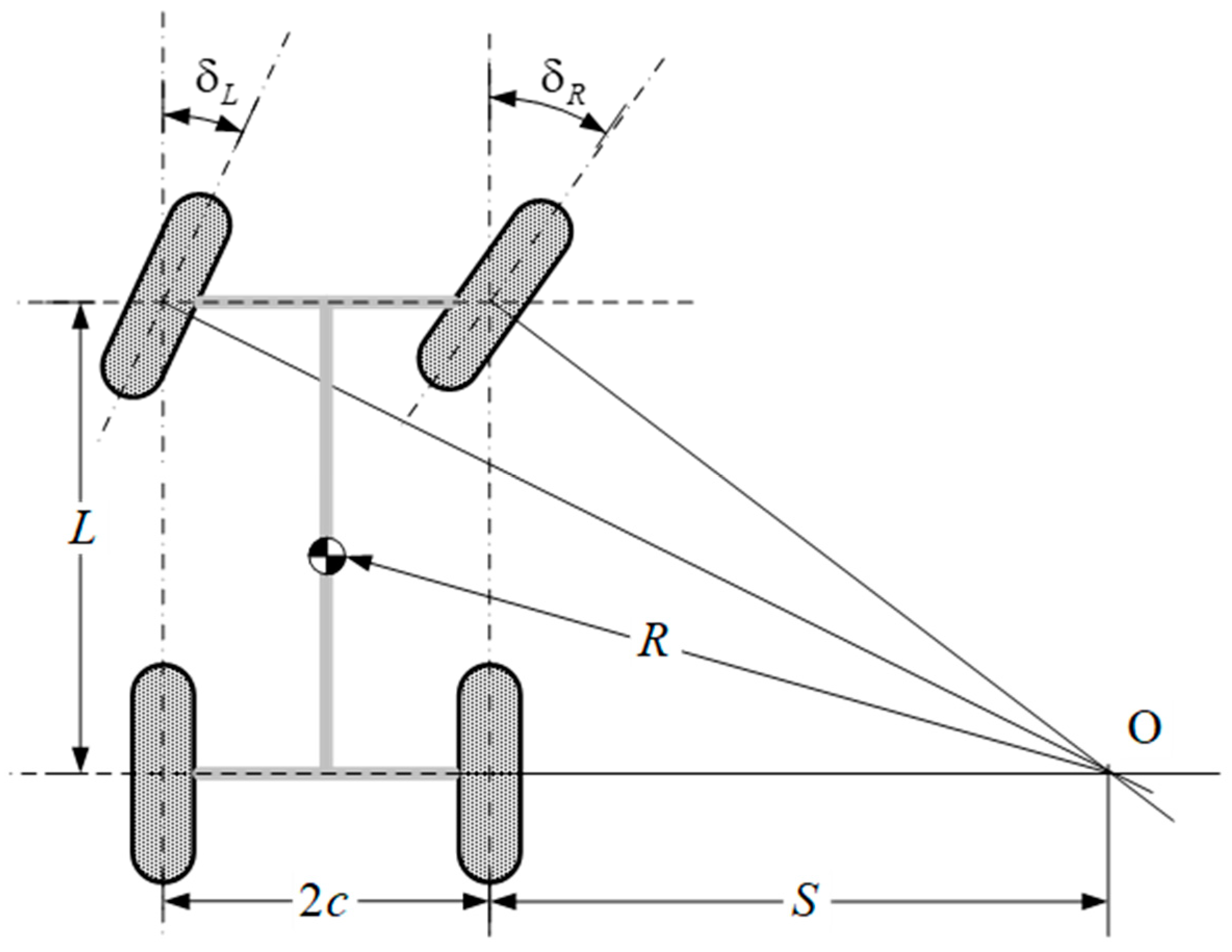
The conditions for executing the turn by rotating the planes of the wheels that belong to the same axle are taken from the kinematics of the turning of the vehicles [36,37,38]. The parameters that define the kinematics are determined based on the scheme in Figure 3 (adapted from [39]), using the following relations:
where O is the instantaneous center of rotation.
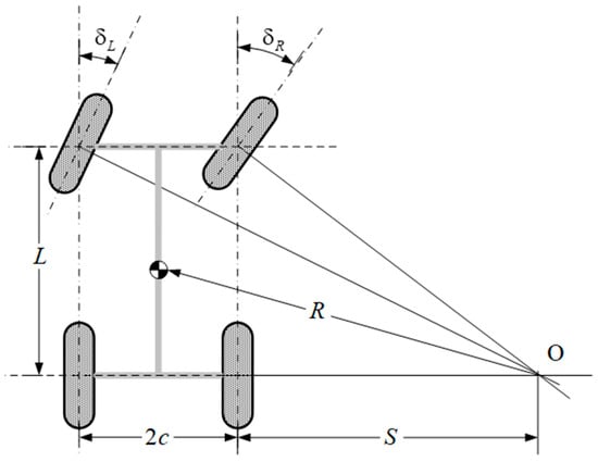
Figure 3.
Diagram of the kinematics of the Ackerman turning system (adapted from [39]).
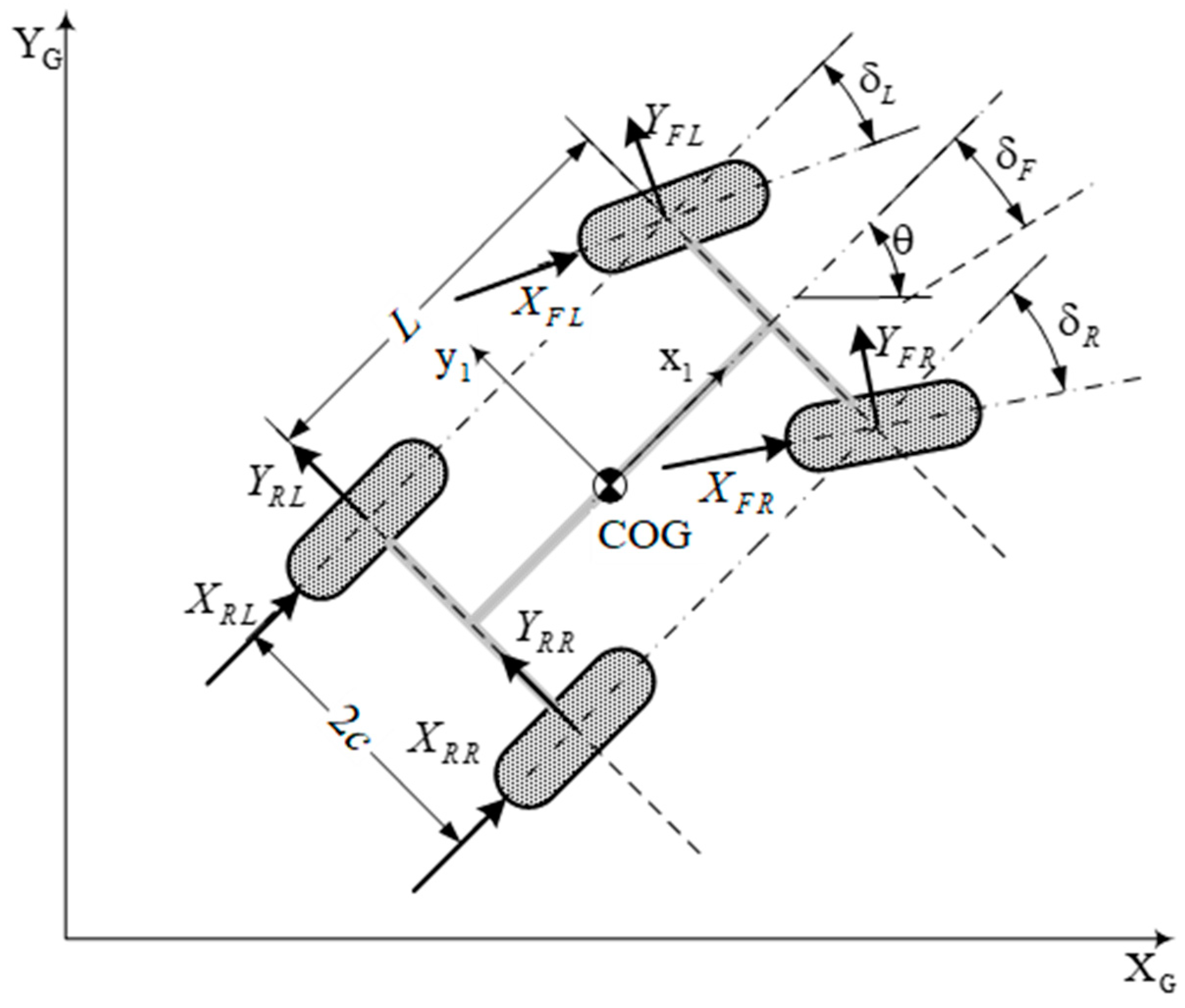
The diagram of the kinematic parameters, as well as the forces acting on the robot, is presented in Figure 4.
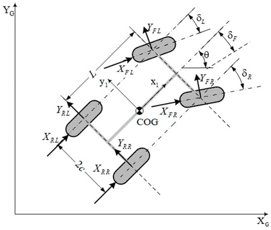
Figure 4.
Calculation scheme for the dynamics of a four-wheeled robot (adapted from [30]).
The robot’s trajectory is defined if its angular acceleration is known relative to the following fixed coordinate system:
The longitudinal forces depend mainly on the moments applied via the electric motors to overcome the forward resistances (rolling resistance, slope resistance, and acceleration resistance), while the transverse forces depend on the cornering conditions, i.e., on the angles of turns denoted as .
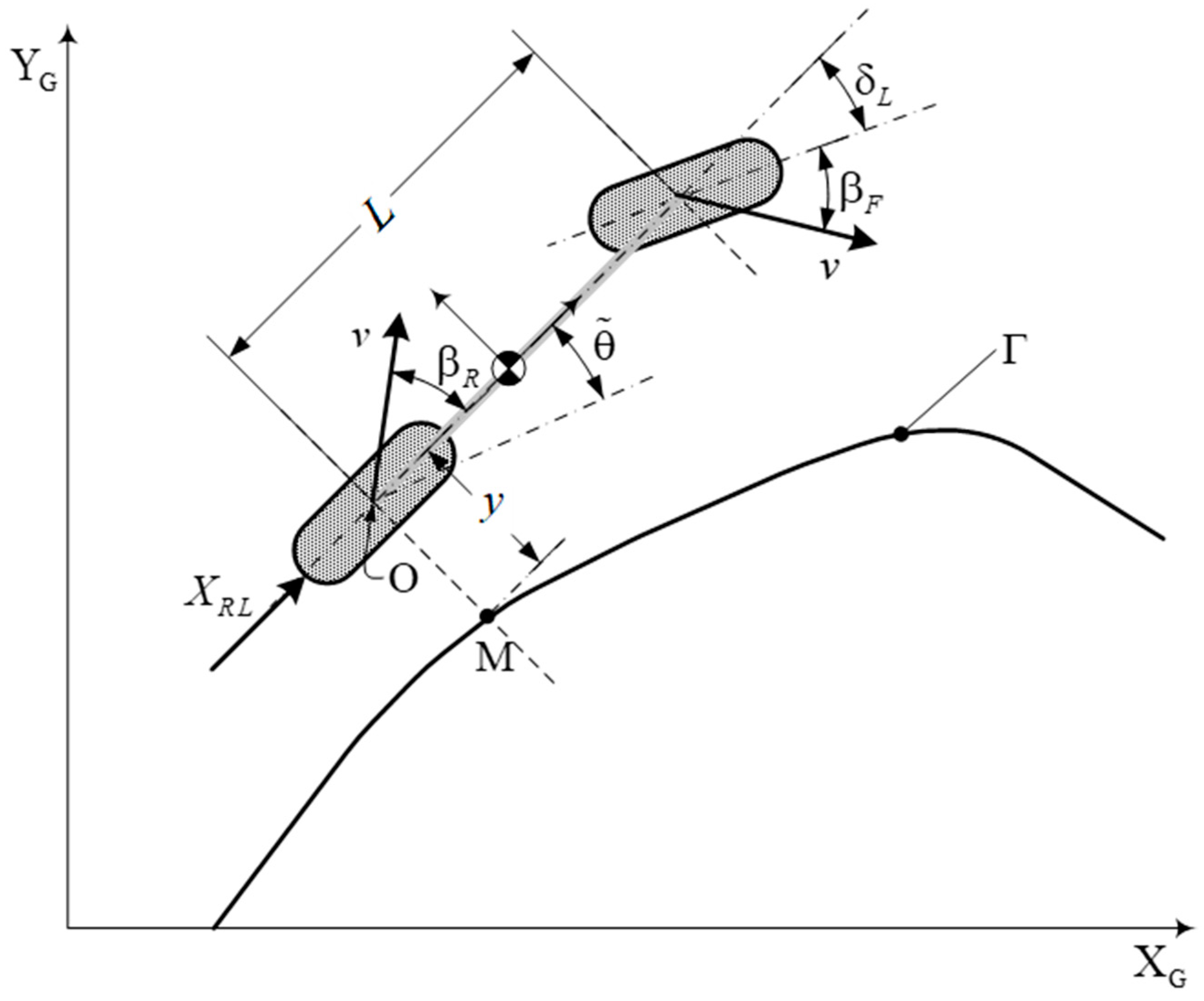
If slips are taken into consideration, as a result of the introduction of lateral slip angles, denoted as , the model can be reduced to the simplified form with only two wheels (Figure 5), where O is the center of the rear wheel subject to the trajectory control action , is the angular deviation from the trajectory , and M is the point located on the trajectory at the smallest distance from O (this point is considered unique).
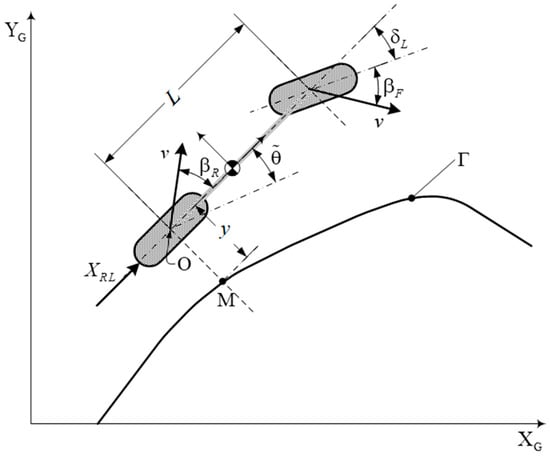
Figure 5.
The simplified kinematic and dynamic model (adapted from [30]).
Based on these notations, the relationships that describe the robot’s kinematics are written as follows [30,31,32,33]:
where and .
The determination of the lateral deviation angles is carried out by initially determining an estimated value that serves as an input variable for an iterative process implemented within the controller [34].
4. Kinematics and Dynamics Study of Four-Wheeled Robots That Execute Skid Turning
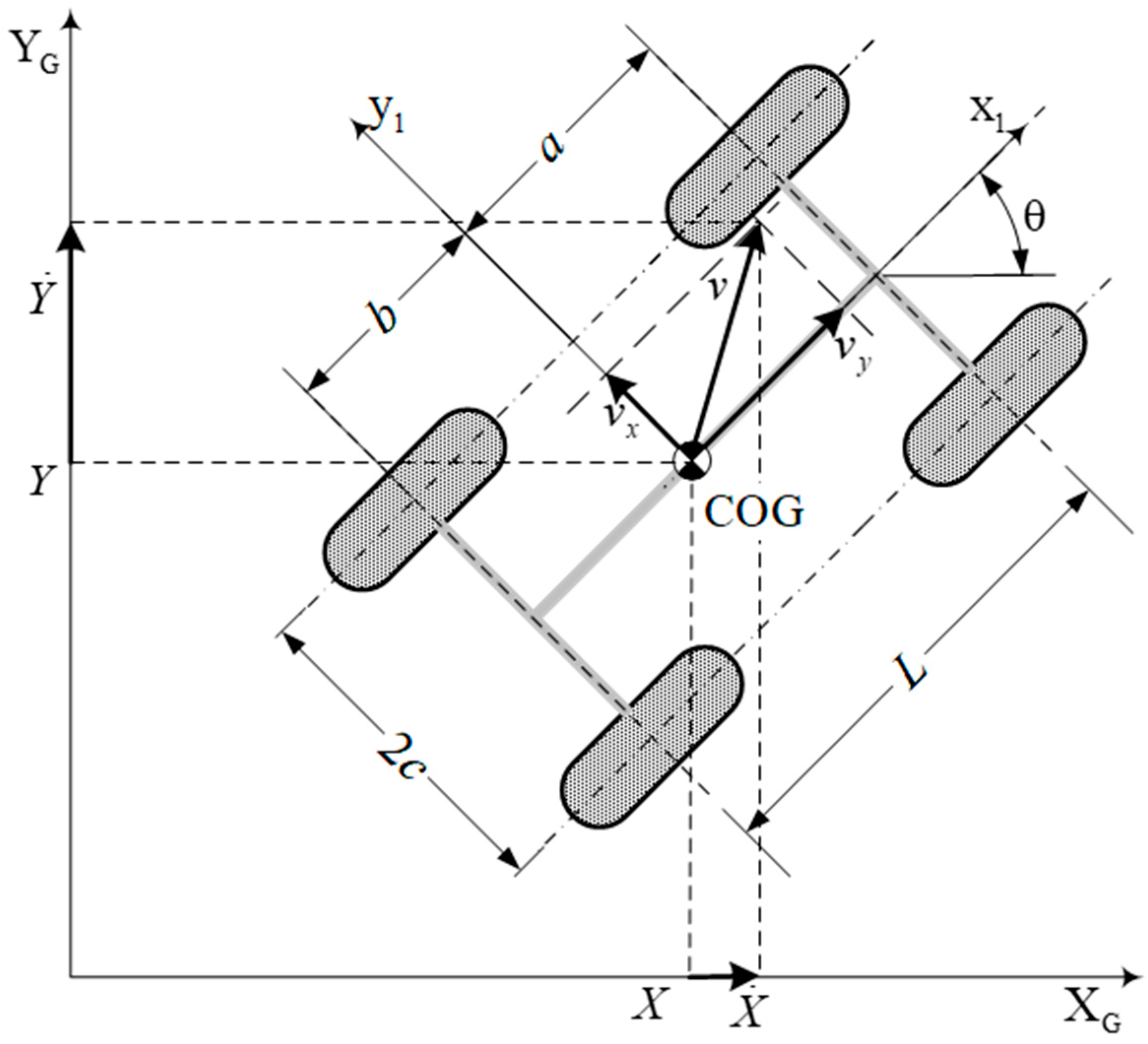
For a four-wheeled robot platform (Figure 6), the absolute speed of the robot, taking into account the hypothesis that it executes a planar movement, is determined using the relation [28] , and the angular velocity with the relation [28] .
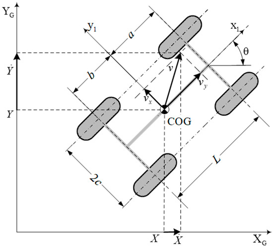
Figure 6.
Center of gravity velocity diagram [28].
If the state vector is , then the velocity vector has the components , as presented schematically in Figure 6.
Since the robot executes a planar motion, the velocities and the angular velocity in the inertial frame of reference (XG, YG) become as follows:
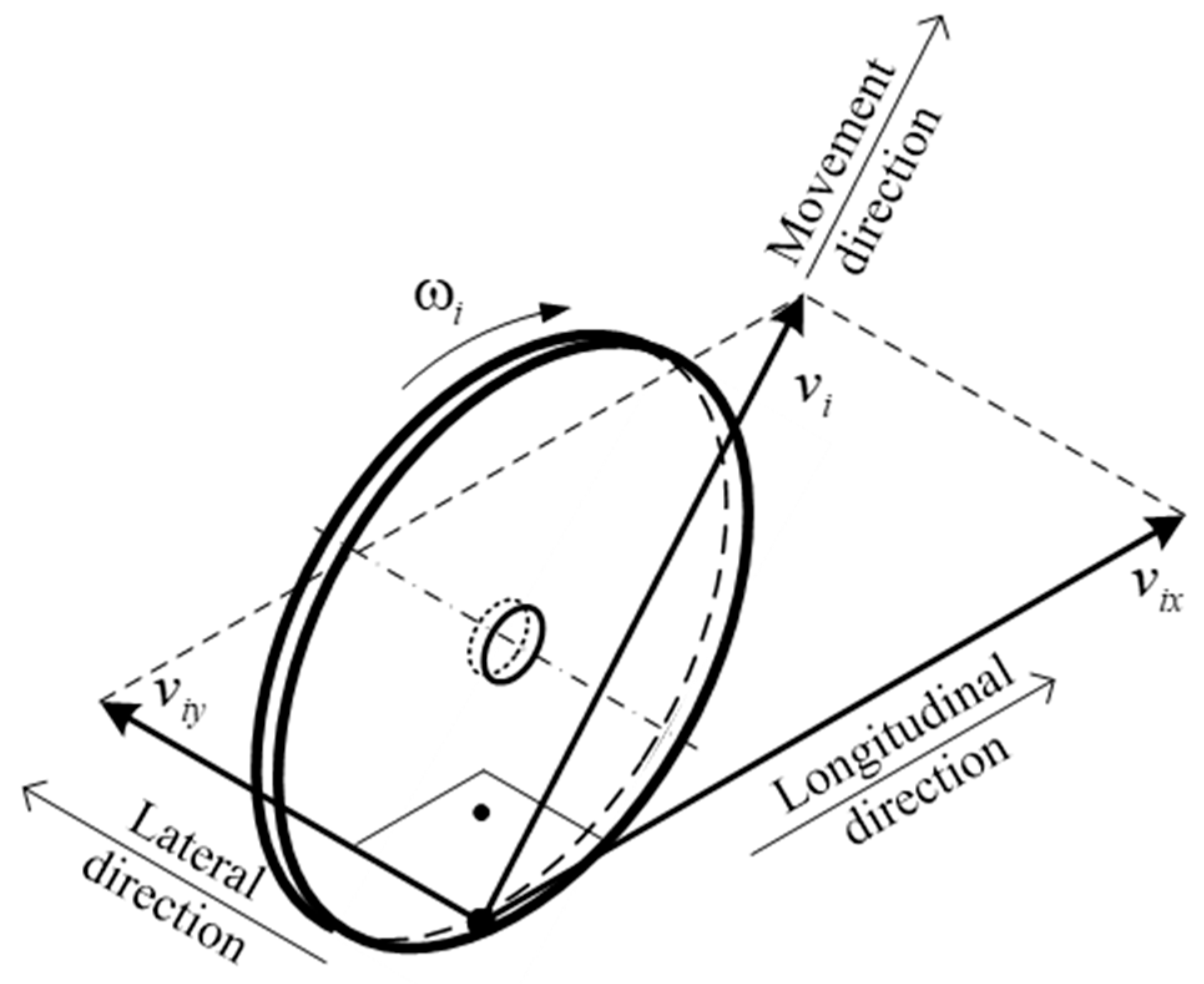
Assuming no longitudinal slippage of the wheel (Figure 7), the longitudinal speed of the wheel (i) is given in the relationship , where (ri) is the wheel radius.

Figure 7.
Wheel velocities (adapted from [28]).
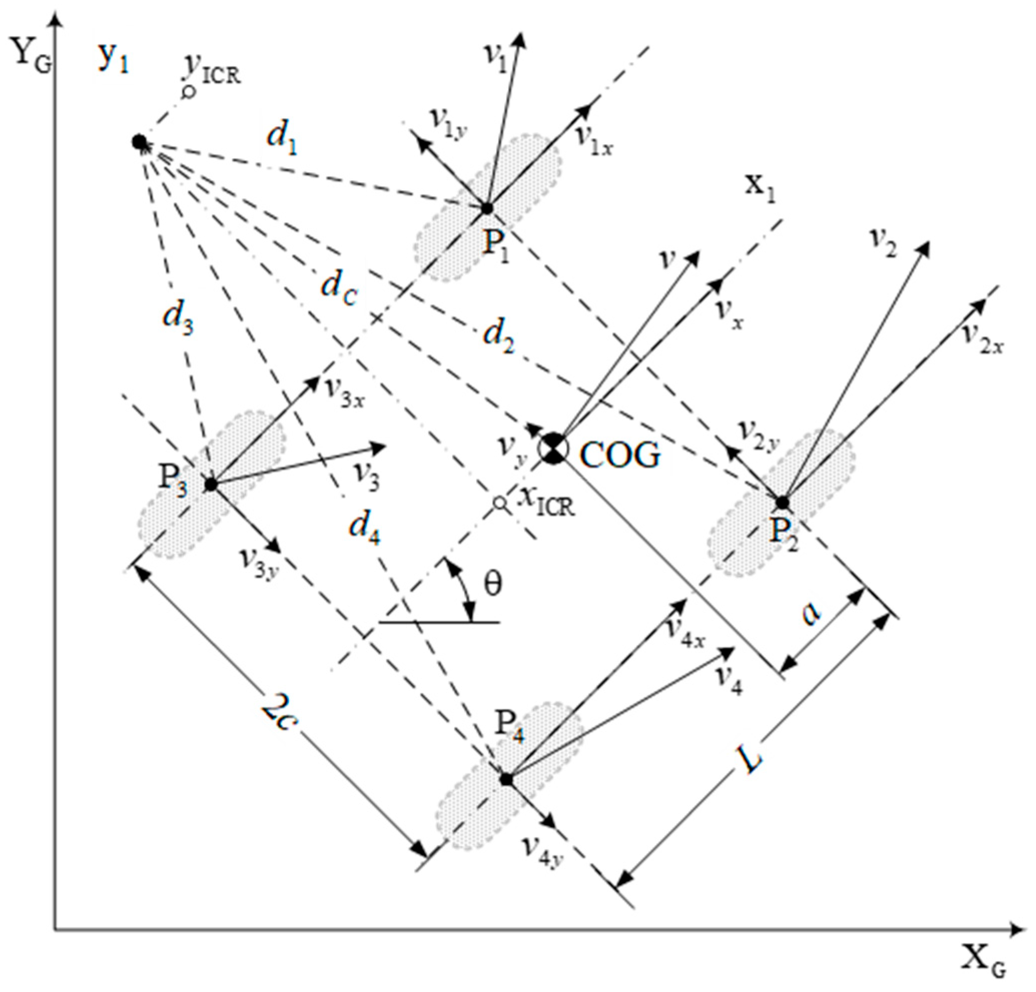
The velocities of all wheels are schematically represented in Figure 8, where ICR is the instantaneous center of rotation, located at the intersection of the perpendiculars to the speed vectors of the four wheels, and COG is the center of mass of the platform, to which the coordinate system is associated.
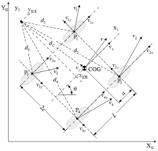
Figure 8.
Diagram for the kinematics of a four-wheeled robot (adapted from [28]).
The vectors of the wheel centers can be defined using their projections , and the position vector of the center of gravity relative to the instantaneous center of rotation is .
The angular velocity of the robot can be written in the following forms:
We consider the coordinates of the center of gravity in the moving frame of reference, and it follows that the relation can be introduced , and, consequently, the expression of the angular velocity takes the following form: .
From the schematization presented in Figure 8, the following relations may be obtained:
By combining the above relations, we finally obtain the following relations for the velocities:
The above relations can be written condensed in the following form [28]:
Consequently, it can be concluded that the above relationship establishes the connection between the wheel speed and the longitudinal speed of the robot, respectively, and the angular speed [40].
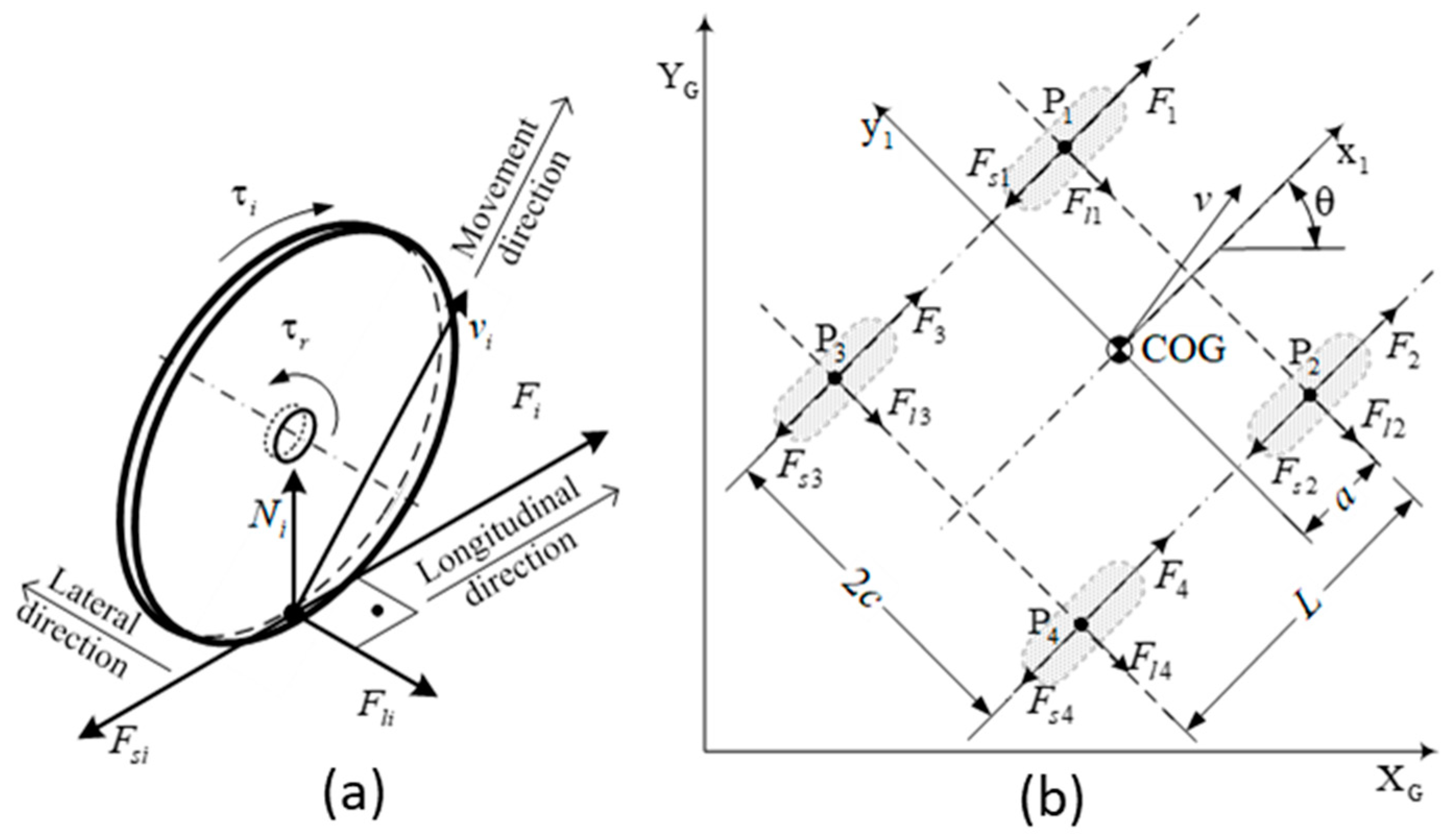
The proposed dynamic model for a four-wheeled robot performing a skid turn aims to evaluate the forces acting on the wheels and, via summation, on the entire robot. The forces acting on one wheel are detailed in Figure 9a, and those acting on all wheels of the robot platform are shown in Figure 9b.
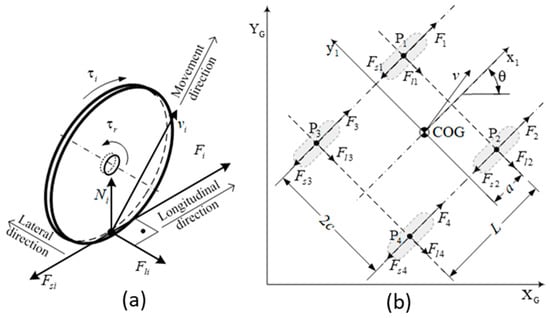
Figure 9.
(a) Forces acting on a wheel; (b) the forces acting on a four-wheeled robot (adapted from [28]).
We assume that the vector results from the rolling resistant moment , and the vector denotes the lateral reactive force.
The longitudinal forces acting on the wheels depend on the moments applied to them via the electric motors, and they are calculated with the following relation:
The normal forces on the roadway and acting on the wheels obey the following relations:
The above relationships form a system that allows the normal forces to be determined as follows:
Lateral forces are considered to result from the Coulombic friction of the wheel with the roadway plus the viscous friction , where is the linear speed, and (N) is the force perpendicular to the surface.
Given the planar motion of the robot, the potential energy variation is zero, so the kinetic energy of the robot is defined with the following relation:
Because , the following expression for the kinetic energy of the robot may be yielded: [28].
Applying the Lagrange method, the derivatives of the total energy of the robot are calculated to determine the inertial forces as follows:
where .
The components in the inertial system of the forces acting on the wheels are expressed as follows:
Consequently, the resisting moment generated by these forces relative to the center of mass is determined via the following relation:
For the approximation of resistance forces, the vector of generalized resistance forces is defined with the relation:
The components of the traction forces in the inertial frame of reference and the active moment that allows the turn to be executed are determined using the following relationship:
It follows that the vector of active forces has the following expression:
Considering that all wheels have the same rolling radius, the vector of active forces becomes as follows:
The notation is introduced, where indices (L) and (R), respectively, refer to the wheels on the left and right side of the robot, and the condensed form is obtained , where (B) denoted the following transformation matrix: .
This results in the following condensed form describing the dynamic model of the robot [28]:
The dynamic model leads to a simple expression of the equation that allows for the determination of the accelerations of the robot according to the moments applied to the wheels. To determine the resistance forces, the model does not take into account the characteristics of the terrain on which the movement is performed.
5. Kinematics and Dynamics Study of Tracked Robots
Characteristics related to the kinematics and dynamics of small-sized tracked propulsion systems are developed starting from the kinematics and dynamics of large-sized tracked vehicles, especially military-tracked vehicles [20,25,26].
For wheeled and tracked vehicles traversing unstructured terrain [1,22,27], approaches based on the generalized Newton Raphson (GNR) method are proposed for the exhaustive identification of the unknown soil parameters necessary to predict the ground force traction [42]. This method takes into account the track slip, soil cohesion, angle of internal soil friction, and soil shear modulus.
The proposed model depends on the soil characteristics and the interaction of the track with the terrain. Thus, for the calculation of the forward resistance and the traction force, the following relations are used:
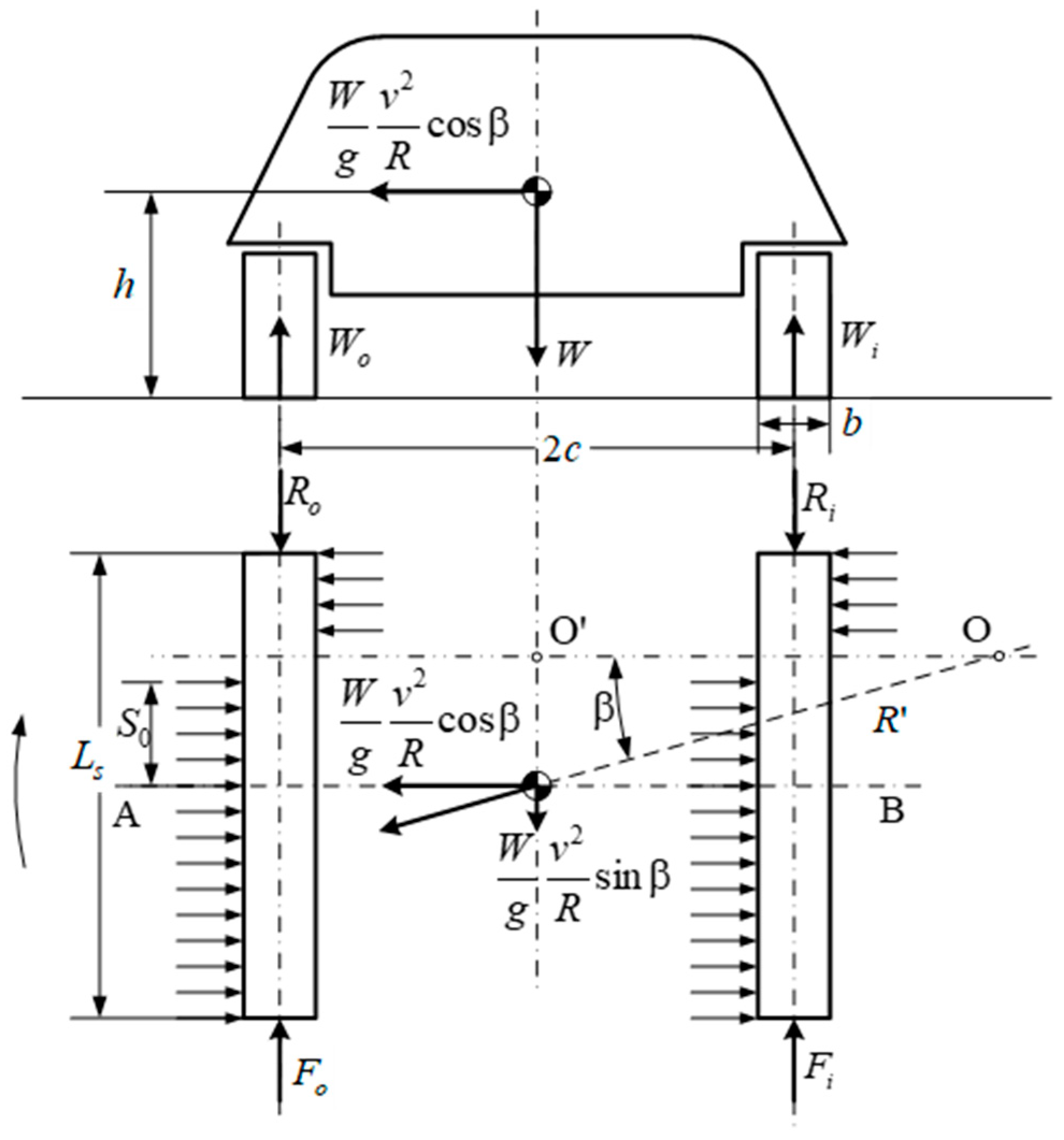
The diagram of the forces and moments acting on a tracked robot during turning is shown in Figure 10.
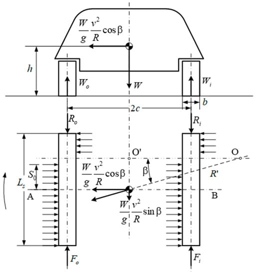
Figure 10.
Diagram of the forces and moments acting on a tracked robot during a turn (adapted from [25]).
The traction forces applied to the two tracks have the following expressions [25]:
where is centrifugal acceleration: ; (V) is longitudinal speed; is longitudinal and transverse resistance coefficients; is the displacement of the turning center expressed as .
The cornering resisting moment is expressed as follows:
The longitudinal resistance coefficient is determined with the relation , or with the empirical relationship , where , where (CI) is the conic index.
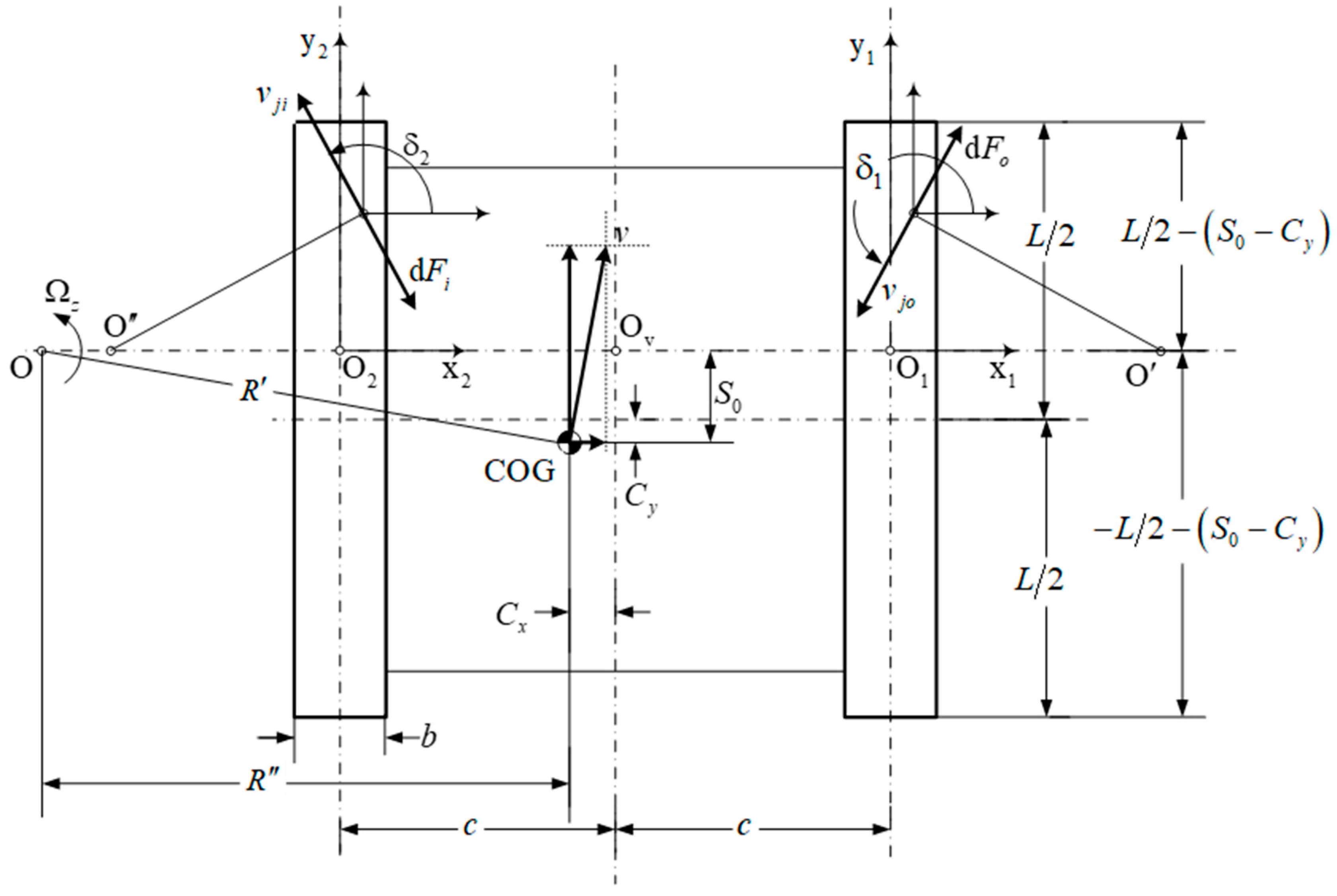
The general diagram of the forces and moments acting on a tracked robot is shown in Figure 11 [25].
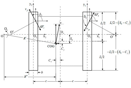
Figure 11.
Calculation scheme for robot kinematics and dynamics (adapted from [25]).
The center of gravity is displaced from the center of symmetry. Also, on the two tracks, two elementary surfaces are considered that slide in relation to the running path.
Under uniform turning conditions, the displacements in the two directions of the fixed X-Y reference system are calculated using the following relations [26]:
The resultant displacement is determined using the following relation:
The relations for the inside track of the turn are also written similarly as follows:
The resultant displacement is determined using the following relation:
The elementary forces acting on the two surfaces considered are expressed as follows:
For the calculation of the unit shear stress, the following generalized relation is used:
The longitudinal forces and the forces in the transverse direction are calculated via the following integration:
The resisting bending moments generated via the longitudinal forces are calculated with the following relations:
Similarly, the resisting moments due to transverse forces are determined as follows:
Angles are determined using the following [25]:
In order to determine the transverse resistance coefficient that intervenes in the relationship with the determination of the resisting moment in the turn, it has to proceed to equalize the resisting moment in the turn with the sum of the resisting moments in the turn generated via the transverse forces as follows:
Eventually, we yield the following equation:
Solving the above equation allows us to calculate the moment of resistance to steering using Equation (22).
This model is based on the basic equations of terramechanics, so it requires knowing the coefficients that allow for the determination of the physical–mechanical characteristics of the soil [43,44]. The real-time determination of soil parameters and their correction within the model leads to improved estimation accuracy and improved trajectory control estimation capability.
6. Conclusions
Within this present work, the kinematic and dynamic models for wheeled and tracked robots were identified and analyzed. The model for estimating the kinematics and dynamics of tracked robots takes into account the physicomechanical characteristics of the ground, the influence of the center of gravity displacement on the cornering moment of resistance, and the interaction of the track with the terrain.
During the development of the model, simplifying calculation assumptions are imposed by which the track is considered to be rigid, the turn is made uniformly and at a constant speed, and the terrain is considered horizontal. Also, for the determination of the resistance forces and the traction force, specific calculation relations of the Wong model and those of the Bekker model for the experimental determination of soil characteristics are used. Consequently, the model requires prior knowledge of the physical–mechanical characteristics of the soil.
The results of the model are characterized by defining the computational relations for a robot’s equations of motion, longitudinal forces, transverse forces, and resistive turning moments generated via longitudinal forces and transverse forces. In the case of tracked robots, some of the power from the inner track is transmitted to the outer track during a turn, thus relieving the traction motor.
The proposed models for estimating the kinematics and dynamics of wheeled robots are specific to four-wheeled robots where turning is achieved by turning the steering wheels or skidding (as in the case of tracked robots). The imposed goal is to determine the radius of the trajectory in the turn knowing the angular velocities of the two tracks or groups of wheels and the position of the planes of the drive wheels, respectively, to determine the forces and moments that load the wheels and the entire robot as a whole.
The execution of a turn via skidding is carried out under the assumption that the wheels keep their plane of symmetry unchanged, the turning radius depends on the speeds of the wheels on the two sides of the robot, and the turning process is accompanied by the lateral skidding of the wheels.
Consequently, due to the influence of the physicomechanical characteristics of the soil on the turning process, a strong correlation between the kinematic and dynamic modes is required. Under these conditions, the dynamic model results in the determination of the expressions for the forces and moments at the wheels, which are later used as input data via the kinematic model to estimate the longitudinal and lateral slips, and based on these, the characteristics of the robot’s trajectory are determined.
In the case of models for robots that perform a turn by turning the directional wheels, the trajectory characteristics depend only on the dimensions and kinematics of the wheel drive and have a weak correlation with the dynamic model, assuming the pure rolling of the wheels, with no longitudinal or lateral slips. Hence, in this case, it is noted that the longitudinal forces depend mainly on the moments applied via the electric motors to overcome the forward resistances, while the transverse forces depend on the cornering conditions, i.e., on the steering angles of the wheels. The trajectory of the robot is given in the centrifugal acceleration of the robot and depends on the longitudinal forces, transverse forces, and steering angles of the wheels.
The proposed models do not take into account the longitudinal slips due to the small size and weight of the configurations of the robotic platforms, but they deal with the problem of the transversal slips of the propulsion system and, consequently, provide the ability to estimate the deviation of the actual trajectory from the theoretical trajectory when walking straight and during turning. Moreover, from the point of view of computational convenience, the models provide relatively simple computational relationships that can be easily implemented in wheeled and tracked robot trajectory estimation algorithms.
Considering models for estimating the kinematics and dynamics of wheeled and tracked ground robots, which consider the physicomechanical characteristics of the ground, we propose, for the future, the instrumenting of ground robots with a system to identify the track profile and position of the center of gravity, which changes due to sinking. Through this sensor system, the sensor system for navigation will be completed, and the validation will be conducted by making a fleet of two robots, one on wheels and one on tracks.
On top of that, we will develop the research starting from the models presented, following their implementation in the NRMM (NATO References Mobility Model) applications (software). Since the mobility of ground robots is becoming as important a topic as the mobility of wheeled and tracked vehicles (including the area of military applications), we will develop a measurement system that will allow us to determine the characteristics of the soils on which we will perform tests.
We also propose an improvement of the models starting from the realization of an analysis process of the interaction of the undercarriage with the ground and from the sensor system that will allow us to identify the position of the robot. With this data, we will make corrections within the formulas used. In this paper, we reviewed the existing models, and we analyzed the kinematics and dynamics of wheeled and tracked vehicles with predefined scenarios. In future research, we intend to create a semi-autonomous/autonomous robot driving system after creating a sensor system to identify the robot’s position and an analysis of the propulsion/deformable terrain interaction. Then, we will use mathematical models that refer to the control theory method.
Author Contributions
Conceptualization, O.A., T.C. and L.Ș.G.; methodology, O.A. and T.C.; software, I.P.; validation, O.A., L.Ș.G. and A.Ș.; formal analysis, A.Ș. and T.L.G.; investigation, T.C.; resources, C.V.; data curation, I.O.; writing—original draft preparation, O.A.; writing—review and editing, I.O.; visualization, C.V.; supervision, O.A.; project administration, I.O. All authors have read and agreed to the published version of the manuscript.
Funding
This work was supported by a grant from the Ministry of Research, Innovation and Digitization, CNCS—UEFISCDI, project number PN-III-P1-1.1-PD-2021-079, within PNCDI III.
Institutional Review Board Statement
Not applicable.
Informed Consent Statement
Not applicable.
Data Availability Statement
Not applicable.
Conflicts of Interest
The authors declare no conflict of interest.
Abbreviations
| Surface area of contact between track and soil | |
| Distance from COG to front axle | |
| Vehicle centrifugal acceleration | |
| Width of the track | |
| Cone index | |
| COG lateral displacement relative to the symmetry center | |
| COG longitudinal displacement relative to the symmetry center | |
| Curvature of the trajectory at point M | |
| Cohesion coefficient | |
| Vehicle tread | |
| Vector of the COG | |
| Vector of the wheel i center, | |
| Longitudinal force acting on the wheel i, | |
| Thrust of the inside track of a tracked vehicle | |
| Thrust of the outside track of a tracked vehicle | |
| Lateral force acting on the wheel i, | |
| Resistance force acting on the wheel i, | |
| Acceleration due to gravity | |
| Height of COG | |
| Moment of inertia of the robot in relation to the center of mass COG | |
| Longitudinal slip of the track | |
| Shear modulus of the soil | |
| Cohesive modulus of terrain deformation | |
| Friction modulus of terrain deformation | |
| Vehicle wheelbase | |
| Length of surface of contact between track and soil | |
| Mass of the vehicle | |
| The normal forces on the roadway acting on the wheel i, | |
| Exponent of terrain deformation | |
| Distance from the instantaneous center of rotation to the COG | |
| Turning radius considering slip | |
| Resistance due to soil compaction | |
| Motion resistance of the inside track of a tracked vehicle | |
| Motion resistance of the outside track of a tracked vehicle | |
| Wheel radius | |
| Turning radius | |
| Displacement of the center of turn | |
| Kinetic energy of the robot | |
| Velocity of vehicle COG | |
| Speed of center of gravity of tracked vehicle | |
| Wheel velocity. Indexes: L—left side; R—right side; F—front wheels; B—rear wheels | |
| Speed of the outer track and the inner track, respectively | |
| Components of vehicle COG velocity in longitudinal and transversal directions, respectively | |
| Speed of the vehicle before steering | |
| Vehicle weight | |
| Longitudinal force acting on wheel. First index: —front wheels; —rear wheels. Second index: —external wheels; —internal wheels. | |
| Lateral force acting on wheel. First index: —front wheels; —rear wheels. Second index: —external wheels; —internal wheels. | |
| Lateral deviation of point O from the trajectory | |
| Vehicle sideslip angle | |
| Lateral slip angles at the front and rear wheels, respectively | |
| External/internal wheel heading (steering angles) | |
| Vehicle heading | |
| Angular deviation from the trajectory | |
| Vehicle heading in presence of wheel slip | |
| Coulomb friction coefficient | |
| Longitudinal resistance coefficient | |
| Viscous friction coefficient | |
| Transverse resistance coefficients | |
| Unit vertical stress of outside and inside track, respectively | |
| Torque acting on wheel i, | |
| Unit share stress of outside and inside track, respectively | |
| Resistant torque acting on wheel i, | |
| Angle of internal shearing resistance | |
| Turning angular speed |
References
- Wong, J.Y. Theory of Ground Vehicles, 3rd ed.; John Willey & Sons: Hoboken, NJ, USA, 2001; ISBN 0-471-35461-9. [Google Scholar]
- Rajamani, R. Vehicle Dynamics and Control, 2nd ed.; Mechanical Engineering Series; Springer: Boston, MA, USA, 2012; ISBN 978-1-4614-1432-2. [Google Scholar] [CrossRef]
- Grigore, L.Ș.; Gorgoteanu, D.; Molder, C.; Alexa, O.; Oncioiu, I.; Ștefan, A.; Constantin, D.; Lupoae, M.; Bălașa, R.-I. A Dynamic Motion Analysis of a Six-Wheel Ground Vehicle for Emergency Intervention Actions. J. Sens. 2021, 21, 1618. [Google Scholar] [CrossRef]
- Huang, D.; Zhai, J.; Ai, W.; Fei, S. Disturbance observer-based robust control for trajectory tracking of wheeled mobile robots. Neurocomputing 2016, 198, 74–79. [Google Scholar] [CrossRef]
- Shojaei, K.; Shahri, A.M.; Tarakameh, A.; Tabibian, B. Adaptive trajectory tracking control of a differential drive wheeled mobile robot. Robotica 2011, 29, 391–402. [Google Scholar] [CrossRef]
- Grigore, L.Ș.; Oncioiu, I.; Priescu, I.; Joița, D. Development and Evaluation of the Traction Characteristics of a Crawler EOD Robot. J. Appl. Sci. 2021, 11, 3757. [Google Scholar] [CrossRef]
- Zhong, Y.; Wang, R.; Feng, H.; Chen, Y. Analysis and research of quadruped robot’s legs: A comprehensive review. Int. J. Adv. Robot. Syst. 2019, 16, 1729881419844148. [Google Scholar] [CrossRef]
- Huang, W.; Xiao, J.; Zeng, F.; Lu, P.; Lin, G.; Hu, W.; Lin, X.; Wu, Y. A Quadruped Robot with Three-Dimensional Flexible Legs. J. Sens. 2021, 21, 4907. [Google Scholar] [CrossRef] [PubMed]
- Lakkad, S. Modeling and Simulation of Steering Systems for Autonomous Vehicles. Master’s Thesis, The Florida State University, Tallahassee, FL, USA, 2004. Available online: https://purl.flvc.org/fsu/fd/FSU_migr_etd-3310 (accessed on 15 June 2023).
- Zhang, W. A robust lateral tracking control strategy for autonomous driving vehicles. Mech. Syst. Signal-Process. 2021, 150, 107238. [Google Scholar] [CrossRef]
- Siegwart, R.; Nourbakhsh, I.R. Introduction to Autonomous Mobile Robots; Bradford Book; MIT Press: Cambridge, MA, USA; London, UK, 2004; ISBN 0-262-19502-X. [Google Scholar]
- Wu, X.; Xu, M.; Wang, L. Differential speed steering control for four-wheel independent driving electric vehicle. In Proceedings of the IEEE International Symposium on Industrial Electronics, Taipei, Taiwan, 28–31 May 2013; pp. 1–6. [Google Scholar] [CrossRef]
- Muir, P.F.; Neuman, C.P. Kinematic Modeling of Wheeled Mobile Robots; Technical Report CMU-RI-TR-86-12; The Robotics Institute, Carnegie-Mellon University: Pittsburg, PA, USA, 1986; Available online: https://www.ri.cmu.edu/pub_files/pub3/muir_patrick_1986_1/muir_patrick_1986_1.pdf (accessed on 10 June 2023).
- Yan, C.; Shao, K.; Wang, X.; Zheng, J.; Liang, B. Reference Governor-Based Control for Active Rollover Avoidance of Mobile Robots. In Proceedings of the 2021 IEEE International Conference on Systems, Man, and Cybernetics (SMC), Melbourne, Australia, 17–20 October 2021; pp. 429–435. [Google Scholar] [CrossRef]
- Jeon, H.; Lee, D. Explicit Identification of Pointwise Terrain Gradients for Speed Compensation of Four Driving Tracks in Passively Articulated Tracked Mobile Robot. Mathematics 2023, 11, 905. [Google Scholar] [CrossRef]
- Fekih, A.; Seelem, S. Effective fault-tolerant control paradigm for path tracking in autonomous vehicles. Syst. Sci. Control Eng. 2015, 3, 177–188. [Google Scholar] [CrossRef]
- Chen, C.-Y.; Li, T.-H.S.; Yeh, Y.-C.; Chang, C.-C. Design and implementation of an adaptive sliding-mode dynamic controller for wheeled mobile robots. Mechatronics 2009, 19, 156–166. [Google Scholar] [CrossRef]
- Domina, Á.; Tihanyi, V. Model Predictive Controller Approach for Automated Vehicle’s Path Tracking. Sensors 2023, 23, 6862. [Google Scholar] [CrossRef]
- Apostolopoulos, D.S. Analytical Configuration of Wheeled Robotic Locomotion. CMU-RI-TR-01-08. Ph.D. Thesis, The Robotics Institute, Carnegie Mellon University, Pittsburgh, PA, USA, April 2001. Available online: https://www.ri.cmu.edu/pub_files/pub2/apostolopoulos_dimitrios_2001_1/apostolopoulos_dimitrios_2001_1.pdf (accessed on 10 June 2023).
- Ciobotaru, T. Engineering of Military Tracked Vehicles, II, Mobility, Tracked Propeller; Publishing House Military Technical Academy Ferdinand I: Bucharest, Romania, 2019; ISBN 978-973-640-296-8. [Google Scholar]
- Golconda, S. Steering Control for a Skid-Steered Autonomous Ground Vehicle at Varying Speed. Master’s Thesis, University Louisiana at Lafayette, Lafayette, LA, USA, 2005. [Google Scholar]
- Hutangkabodee, S.; Zweir, Y.H.; Seneviratne, L.D.; Althoefer, K. Validation of Soil Parameter Identification for Track-Terrain Interaction Dynamics. In Proceedings of the 2007 IEEE/RSJ International Conference on Intelligent Robots and Systems, San Diego, CA, USA, 29 October–2 November 2007. [Google Scholar] [CrossRef]
- Martinez, J.L.; Mandow, A.; Morales, J.; Pedraza, S.; Garcia-Cerezo, A. Approximating Kinematics for Tracked Mobile Robots. Int. J. Robot. Res. 2005, 24, 867–878. [Google Scholar] [CrossRef]
- Lin, L.; Xu, Z.; Zheng, J. Predefined Time Active Disturbance Rejectionfor Nonholonomic Mobile Robots. Mathematics 2023, 11, 2704. [Google Scholar] [CrossRef]
- Said, A.-M.; Seneviratne, L.D.; Althoefer, K. Track–terrain modelling and traversability prediction for tracked vehicles on soft terrain. J. Terramech. 2010, 47, 151–160. [Google Scholar] [CrossRef]
- Amar, F.B.; Grand, C.; Besseron, G.; Lhomme-Desages, D.; Lucet, E. Mobility and stability of robots on rough terrain: Modeling and control. In Proceedings of the IROS, Kompai Robotics, Nice, France, 22–26 September 2008; Available online: https://kompairobotics.com/wp-content/uploads/2018/12/32.pdf (accessed on 11 June 2023).
- Hutangkabodee, S.; Zweir, Y.H.; Seneviratne, L.D.; Althoefer, K. Soil Parameter Identification and Driving Force Prediction for Wheel-Terrain Interaction. Int. J. Adv. Robot. Syst. 2008, 5, 425–432. [Google Scholar] [CrossRef]
- Kozłowski, K.; Pazderski, D. Modeling and control of a 4-wheel skid-steering mobile robot. Int. J. Math. Comput. Sci. 2004, 14, 477–496. Available online: https://eudml.org/doc/207713 (accessed on 8 June 2023).
- Lenain, R.; Thuilot, B.; Cariou, C.; Martinet, P. Mixed kinematic and dynamic sideslip angle observer for accurate control of fast off-road mobile robots. J. Field Robot. 2010, 27, 181–196. [Google Scholar] [CrossRef]
- Lenain, R.; Lucet, E.; Grand, C.; Thuilot, B.; Amar, F.B. Accurate and stable mobile robot path tracking: An integrated solution for off-road and high speed context. In Proceedings of the IEEE/RSJ International Conference on Intelligent Robots and Systems, Taipei, Taiwan, 18–22 October 2010. [Google Scholar] [CrossRef]
- Lenain, R.; Thuilot, B.; Cariou, C.; Martinet, P. High accuracy path tracking for vehicles in presence of sliding: Application to farm vehicle automatic guidance for agricultural tasks. Auton. Robot. 2006, 21, 79–97. [Google Scholar] [CrossRef]
- Cariou, C.; Lenain, R.; Thuilot, B.; Martinet, P. Adaptive control of four-wheel-steering off-road mobile robots: Application to path tracking and heading control in presence of sliding. In Proceedings of the IEEE Eplore International Conference IROS 2008: Intelligent Robots and Systems, Nice, France, 22–26 September 2008. [Google Scholar] [CrossRef]
- Cariou, C.; Lenain, R.; Thuilot, B.; Martinet, P. Path following of a vehicle-trailer system in presence of sliding: Application to automatic guidance of a towed agricultural implement. In Proceedings of the 2010 IEEE/RSJ International Conference on Intelligent Robots and Systems, Taipei, Taiwan, 18–22 October 2010. [Google Scholar] [CrossRef]
- Viana, Í.B.; Kanchwala, H.; Ahiska, K.; Aouf, N. A Comparison of Trajectory Planning and Control Frameworks for Cooperative Autonomous Driving. J. Dyn. Syst. Meas. Control 2021, 143, 71002. [Google Scholar] [CrossRef]
- Mandow, A.; Martinez, J.L.; Morales, J.; Blanco, J.L.; Garcia-Cerezo, A.; Gonzalez, J. Experimental Kinematics for Wheeled Skid-Steer Mobile Robots. In Proceedings of the IEEE/RSJ International Conference on Intelligent Robots and Systems, San Diego, CA, USA, 29 October–2 November 2007; pp. 1222–1227. [Google Scholar] [CrossRef]
- Tagne, G.; Talj, R.; Charara, A. Higher-order sliding mode control for lateral dynamics of autonomous vehicles, with experimental validation. In Proceedings of the 2013 IEEE intelligent vehicles symposium (IV), Gold Coast, Australia, 23–26 June 2013. [Google Scholar] [CrossRef]
- Revueltas, L.; Santos-Sánchez, O.-J.; Salazar, S.; Lozano, R. Optimizing Nonlinear Lateral Control for an Autonomous Vehicle. J. Veh. 2023, 5, 978–993. [Google Scholar] [CrossRef]
- Katriniok, A.; Maschuw, J.P.; Christen, F.; Eckstein, L.; Abel, D. Optimal vehicle dynamics control for combined longitudinal and lateral autonomous vehicle guidance. In Proceedings of the 2013 European Control Conference (ECC), Zurich, Switzerland, 17–19 July 2013; pp. 974–979. [Google Scholar] [CrossRef]
- Shamah, B. Experimental Comparison of Skid Steering vs. Explicit Steering for a Wheeled Mobile Robot. Master’s Thesis, The Robotics Institute, Carnegie Mellon University, Pittsburgh PA, USA, 1999. Available online: https://www.ri.cmu.edu/pub_files/pub1/shamah_benjamin_1999_1/shamah_benjamin_1999_1.pdf (accessed on 12 June 2023).
- Xu, Y.; Tang, W.; Chen, B.; Qiu, L.; Yang, R. A Model Predictive Control with Preview-Follower Theory Algorithm for Trajectory Tracking Control in Autonomous Vehicles. Symmetry 2021, 13, 381. [Google Scholar] [CrossRef]
- Wei, Y.; Collins, E.; Chuy, O. Dynamic Modeling and Power Modeling of Robotic Skid-Steered Wheeled Vehicles. In Proceedings of the 2009 IEEE/RSJ International Conference on Intelligent Robots and Systems, St. Louis, MO, USA, 10–15 October 2009; pp. 4212–4219. [Google Scholar] [CrossRef]
- Wong, J.Y.; Chiang, C.F. A general theory for skid steering of tracked vehicles. Proc. Inst. Mech. Eng. Part D J. Automob. Eng. 2001, 215, 343–355. [Google Scholar] [CrossRef]
- Wong, J.Y. Terramechanics and Off-Road Vehicle Engineering: Terrain Behaviour, Off-Road Vehicle Performance and Design, 2nd ed.; Publish Butterworth Heinemann: Oxford, UK, 2009; p. 488. ISBN 978-0-75-068561-0. [Google Scholar] [CrossRef]
- Ciobotaru, T. Semi-Empiric Algorithm for Assessment of the Vehicle Mobility. Leonardo Electron. J. Pract. Technol. 2009, 8, 19–30. Available online: https://lejpt.academicdirect.org/A15/019_030.pdf (accessed on 12 June 2023).

Disclaimer/Publisher’s Note: The statements, opinions and data contained in all publications are solely those of the individual author(s) and contributor(s) and not of MDPI and/or the editor(s). MDPI and/or the editor(s) disclaim responsibility for any injury to people or property resulting from any ideas, methods, instructions or products referred to in the content. |
© 2023 by the authors. Licensee MDPI, Basel, Switzerland. This article is an open access article distributed under the terms and conditions of the Creative Commons Attribution (CC BY) license (https://creativecommons.org/licenses/by/4.0/).