On a Generalized Wave Equation with Fractional Dissipation in Non-Local Elasticity

Abstract

We analyze wave equation for spatially one-dimensional continuum with constitutive equation of non-local type. The deformation is described by a specially selected strain measure with general fractional derivative of the Riesz type. The form of constitutive equation is assumed to be in strain-driven type, often used in nano-mechanics. The resulting equations are solved in the space of tempered distributions by using the Fourier and Laplace transforms. The properties of the solution are examined and compared with the classical case.

1. Introduction

Differential equations of fractional orders appear in many branches of physics and mechanics. There are numerous solutions to concrete problems collected in the books [1,2,3,4,5,6], for example. Fractional derivatives (FDs) are non-local operators, and, in most applications in mechanics, fractional derivatives, when the independent coordinate is time, are used to model the dissipation and/or memory in the system. If FDs are used to describe memory, physically they represent the (fading) memory of the system. However, when spatial coordinates are used as independent variables, the fractional derivatives model non-local action. As is well known in nano-materials, the non-local action (see [7]) is an important phenomenon that is used to explain many properties that are characteristic of such materials. In solid mechanics in general, and non-local and nano-mechanics in particular, there are two types of constitutive equations that are used: strain- and stress-driven constitutive equations. In the strain-driven form of constitutive equation, that we use in this work, the stress is determined by action of a non-local operator on strain. In this work we shall formulate relevant equations for the spatially one-dimensional body with a linear constitutive equation in a specially selected deformation measure (strain) that is non-local. The use of a general fractional derivative of a displacement field $y(x,t)$ in the form of the so-called truncated power-law kernel (see [8]) is the novelty that we propose here. After we formulate the problem in distributional setting, we shall study some special motions, with the emphasis on wave propagation with or without body forces.

2. Mathematical Model

Consider a rod with straight axis. Let x be a coordinate coinciding with the rod axis. Suppose that the rod occupies a part of the space for which $x\in \left[a,L\right]$, with $a<L.$ We state the definitions of the left and right general fractional derivative (GFD) of the Caputo type (see [9,10]). Throughout, we assume $0<\alpha <1.$ The left GFD derivative of the Caputo type of order $\alpha$ is defined as

$$\left({}_a^C{D}_x^{\alpha ,\lambda }y\right)\left(x\right)=\frac{1}{\mathsf{\Gamma }\left(1-\alpha \right)}{\int }_a^x\frac{exp\left(-\lambda \left(x-\tau \right)\right)y^{\left(1\right)}\left(\tau \right)}{{\left(x-\tau \right)}^{\alpha }}d\tau ,x\in \left(a,L\right),$$

(1)

$$\lambda \ge 0,$$

where $\mathsf{\Gamma }$ is Euler’s gamma function and y is assumed to be absolutely continuous, i.e.,

$$\frac{\partial y\left(x,t\right)}{\partial x}\in L^1,t\ge 0.$$

In writing (1) we used specific kernel $\frac{x^{-\alpha }exp\left(-\lambda x\right)}{\mathsf{\Gamma }\left(1-\alpha \right)},$ suggested for application in continuum mechanics; see [11], p. 6. The kernel $\frac{x^{-\alpha }exp\left(-\lambda x\right)}{\mathsf{\Gamma }\left(1-\alpha \right)}$ is called the truncated power-law kernel and was used earlier for the study of anomalous diffusion in [8] (Equation (2.35)), [12] (Equation (13)) and in [13] (Equation (10)) as a friction kernel for the study of lipid motion in a lipid bilayer system. Similarly, the right GFD derivative of the Caputo type of order $\alpha$ with $0<\alpha <1$ is defined as

$$\left({}_x^C{D}_L^{\alpha ,\lambda }y\right)\left(x\right)=-\frac{1}{\mathsf{\Gamma }\left(1-\alpha \right)}{\int }_x^L\frac{exp\left(-\lambda \left(\tau -x\right)\right)y^{\left(1\right)}\left(\tau \right)}{{\left(\tau -x\right)}^{\alpha }}d\tau ,x\in \left(a,L\right),$$

(2)

$$\lambda \ge 0.$$

Note that $\left({}_a^C{D}_x^{1,\lambda }y\right)\left(x\right)=\frac{dy}{dx}$, $\left({}_x^C{D}_L^{1,\lambda }y\right)\left(x\right)=-\frac{dy}{dx}.$ We need the definitions of Riesz-type GFD. Using (1) and (2), we define

$${\overline{D}}_x^{\alpha ,\lambda }y\left(x\right)=\frac{1}{2}\left[{}_a^C{D}_x^{\alpha ,\lambda }y\left(x\right)-{}_x^C{D}_L^{\alpha ,\lambda }y\left(x\right)\right].$$

(3)

Equation (3) is written as

$${\overline{D}}_x^{\alpha ,\lambda }y\left(x\right)=\frac{1}{2}\frac{1}{\mathsf{\Gamma }\left(1-\alpha \right)}{\int }_a^L\frac{exp\left(-\lambda \left|x-\tau \right|\right)}{{\left|x-\tau \right|}^{\alpha }}{y}^{\left(1\right)}\left(\tau \right)d\tau .$$

(4)

Before we define a new deformation measure, we state the classical strain tensor of linear elasticity (see [14]) that for the three-dimensional body reads

$$E_{ij}\left(x_k,t\right)=\frac{1}{2}\left(\frac{\partial u_i}{\partial x_j}+\frac{\partial u_j}{\partial x_i}\right),i,j,k=1,2,3.$$

(5)

In (5), we denoted by $u_i\left(x_j,t\right)$, $i,j=1,2,3$ components of the displacement vector with respect to a prescribed Cartesian coordinate system with axes $x_j.$ Also, we use t to denote time. Since here we consider one-dimensional bodies only, (5) becomes

$$E\left(x,t\right)=\frac{\partial u\left(x,t\right)}{\partial x}.$$

(6)

Here $u=u_1$ is the only non-zero component of displacement vector. Also, $x=x_1$ is the axis coinciding with the rod axis. Instead of (6), we shall use the following deformation measure

$${\mathcal{E}}^{\alpha ,\lambda }\left(x,t\right)={\overline{D}}_x^{\alpha ,\lambda }u\left(x,t\right).$$

(7)

In (7) we used ${\overline{D}}_x^{\alpha ,\lambda }$ defined by (4). Also, the derivatives are taken with respect to $x.$ We assume that the displacement field is absolutely continuous $u\left(x,t\right)\in AC\left(\mathbb{R}\right)$ in the variable x (absolutely continuous, i.e., $\frac{\partial u\left(x,t\right)}{\partial x}\in L^1,t\ge 0)$. In this case, (1) and (2) exist and

$${\mathcal{E}}^{\alpha ,\lambda }\left(x,t\right)=\frac{1}{2}\frac{1}{\mathsf{\Gamma }\left(1-\alpha \right)}{\int }_a^L\frac{exp\left(-\lambda \left|x-\tau \right|\right)}{{\left|x-\tau \right|}^{\alpha }}\frac{\partial u\left(\tau ,t\right)}{\partial \tau }d\tau ,$$

with $0<\alpha <1$, $\lambda \ge 0$ exists too. The deformation measure, or strain, ${\mathcal{E}}^{\alpha ,\lambda }\left(x,t\right)$ is non-local. Actually ${\mathcal{E}}^{\alpha ,\lambda }\left(x,t\right)$ takes values of the classical strain $\frac{\partial u\left(x,t\right)}{\partial x}$ at all points of the body, with the weighting function equal to $\frac{exp\left(-\lambda \left|x\right|\right)}{{\left|x\right|}^{\alpha }}$.

Remark 1. 

For the case of three-dimensional elasticity theory, one can use the recently defined multidimensional generalized Riesz derivative of the Luchko type, presented in [15], to define generalization of the type (7) for the strain tensor (5).

Next we propose the constitutive equation of the rod. We assume that it is given in strain-driven form, so that with (7) the linear stress-deformation measure relation becomes

$$\sigma \left(x,t\right)=E_0{\mathcal{E}}^{\alpha ,\lambda }\left(x,t\right),$$

(8)

where $\sigma$ is the stress and $E_0$ is a constant (generalized modulus of elasticity). We consider several special cases of (8).

• ${\mathcal{E}}^{\alpha ,0}\left(x,t\right)$ is the strain measure used in [16];
• ${\mathcal{E}}^{1,\lambda }\left(x,t\right)=\frac{\partial u\left(x,t\right)}{\partial x}$, since ${\displaystyle \underset{\alpha \to 1}{lim}}\frac{x^{-\alpha }}{\mathsf{\Gamma }(1-\alpha )}=\delta \left(x\right)$;
• ${\mathcal{E}}^{0,\lambda }\left(x,t\right)$ is the Riesz type of derivative for the Caputo–Fabrizio fractional derivative

  $${\mathcal{E}}^{0,\lambda }\left(x,t\right)={\int }_a^{L}exp\left(-\lambda \left|x-\tau \right|\right)\frac{\partial u\left(\tau ,t\right)}{\partial \tau }d\tau ,$$

  if we take $\lambda =\frac{\alpha }{1-\alpha }$ and add the constant $\frac{2}{1-\alpha }$ in front [17,18].

Suppose that we assume that the displacement field is given as $u\left(x,t\right)=c\left(t\right)$, with $c\left(t\right)$ being arbitrary. This represents the rigid body motion along the axis of the body. Then

$${\mathcal{E}}^{\alpha ,\lambda }\left(x,t\right)=0.$$

Therefore, we conclude that the rigid body motion of the rod, i.e., $u\left(x,t\right)=c\left(t\right)$, with $c\left(t\right)$ being arbitrary, leads to zero strain. This shows that ${\mathcal{E}}^{\alpha ,\lambda }\left(x,t\right)$ can be used as a strain measure. Now we analyze the general problem of motions that result in strain given by (7), that is equal to zero. To do this, we examine the solution to the equation ${\mathcal{E}}^{\alpha ,\lambda }\left(x,t\right)=0$ in general. We consider

$${\int }_a^L\frac{exp\left(-\lambda \left|x-\tau \right|\right)}{{\left|x-\tau \right|}^{\alpha }}\frac{\partial u\left(\tau ,t\right)}{\partial \tau }d\tau =0.$$

(9)

The next Lemma summarizes the result.

Lemma 1. 

For $0<\alpha <1$ the only solution to (9) for $x\in \left(a,L\right)$, $t\ge 0$, is $u\left(x,t\right)=c\left(t\right).$

Proof. 

Let $U\left(x,t\right)$ be a function defined as

$$U\left(x,t\right)=\left\{\begin{array}{cc}\frac{\partial u\left(x,t\right)}{\partial x},& a<x<L,\hfill \\ 0,& x<a\mathrm{or}x>L,\hfill \end{array}\right.t\ge 0.$$

Then

$${\int }_a^L\frac{exp\left(-\lambda \left|x-\tau \right|\right)}{{\left|x-\tau \right|}^{\alpha }}\frac{\partial u\left(\tau ,t\right)}{\partial \tau }d\tau =$$

$$={\int }_{-\infty }^{+\infty }\frac{exp\left(-\lambda \left|x-\tau \right|\right)}{{\left|x-\tau \right|}^{\alpha }}\frac{\partial u\left(\tau ,t\right)}{\partial \tau }d\tau =$$

$$=\left(\frac{exp\left(-\lambda \left|\tau \right|\right)}{{\left|\tau \right|}^{\alpha }}\ast U\left(\tau ,t\right)\right)\left(x,t\right),$$

where ∗ denotes the convolution. Equation (9) now becomes

$$\left(\frac{exp\left(-\lambda \left|\tau \right|\right)}{{\left|\tau \right|}^{\alpha }}\ast U\left(\tau ,t\right)\right)\left(x,t\right)=0,t\ge 0.$$

(10)

Since (10) is an equation represented by convolution of two elements from the space of tempered distribution, one of which is with compact support, we analyze (10) in the space of tempered distribution ${\mathcal{S}}^{\prime }.$ Let $\left[U\left(x,t\right)\right]$ be a regular distribution defined by $U\left(x,t\right).$ $\left[U\left(x,t\right)\right]$ is with the compact support. Distribution $\left[\frac{exp\left(-\lambda \left|\tau \right|\right)}{{\left|\tau \right|}^{\alpha }}\right],$ defined by $\frac{exp\left(-\lambda \left|\tau \right|\right)}{{\left|\tau \right|}^{\alpha }},$ is in ${\mathcal{S}}^{\prime }.$ Consequently, the convolution

$$\left[\frac{exp\left(-\lambda \left|\tau \right|\right)}{{\left|\tau \right|}^{\alpha }}\right]\ast \left[U\left(x,t\right)\right]$$

exists. We now apply the Fourier transform to (10). Firstly, we have, see [19], p. 346,

$$\mathcal{F}\left(\frac{exp\left(-\lambda \left|\tau \right|\right)}{{\left|\tau \right|}^{\alpha }}\right)\left(k\right)=2i\mathsf{\Gamma }(1-\alpha ){\left({\lambda }^2+k^2\right)}^{-\frac{1-\alpha }{2}}cos\left[\left(1-\alpha \right)\mathsf{\Theta }\left(k\right)\right],$$

(11)

where

$$\mathsf{\Theta }\left(k\right)=arctan\frac{k}{\lambda }.$$

(12)

Next, by using (11) in (10) we obtain

$$\left[2i{\left({\lambda }^2+k^2\right)}^{-\frac{1-\alpha }{2}}cos\left[\left(1-\alpha \right)\mathsf{\Theta }\left(k\right)\right]\right]\mathcal{F}\left[U\left(\tau ,t\right)\right]\left(k\right)=0.$$

(13)

Since $\mathcal{F}\left(\left[U\right]\right)\left(k\right)$ is an entire function in $k,t\ge 0,$ from (13) and the uniqueness theorem for the Fourier transform we conclude that $\mathcal{F}\left(U\right)=0$ if $0<\alpha <1,$ or $\frac{\partial u\left(x,t\right)}{\partial x}=0,$ a.e. Thus, $u\left(x,t\right)=c\left(t\right).$ □

We combine (4) and (11) to obtain

$$\mathcal{F}\left({\overline{D}}_x^{\alpha ,\lambda }y\left(x\right)\right)=2i\left|k\right|{\left({\lambda }^2+k^2\right)}^{-\frac{1-\alpha }{2}}cos\left[\left(1-\alpha \right)\mathsf{\Theta }\left(k\right)\right]\mathrm{sgn}\left(k\right)\mathcal{F}\left(y\right)\left(k\right),$$

(14)

where $\mathsf{\Theta }\left(k\right)$ is given by (12).

Equation of motion is

$$\frac{\partial \sigma \left(x,t\right)}{\partial x}+f\left(x,t\right)=\rho \frac{{\partial }^{2}u\left(x,t\right)}{\partial t^2},$$

(15)

where f denotes the prescribed body forces and $\rho$ denotes density. We take body force in the form of friction force, proportional to the Caputo fractional derivative of displacement $u(x,t)$ with respect to time, i.e.,

$$f\left(x,t\right)=-\mu {}_0^C{D}_t^{\beta }u\left(x,t\right)=-\mu \frac{1}{\mathsf{\Gamma }\left(1-\beta \right)}{\int }_0^t\frac{1}{{\left(t-\xi \right)}^{\beta }}\frac{\partial u\left(x,\xi \right)}{\partial \xi }d\xi ,0\le \beta \le 1,$$

(16)

with $\mu \ge 0.$ The form of the body force is taken to be proportional to the Caputo fractional derivative of displacement in order to be able to model viscous force $\beta =1$ and purely elastic resistance force $\beta =0.$ Then, the equation of motion becomes

$$\rho \frac{{\partial }^{2}u}{\partial t^2}=E_0\frac{\partial {\mathcal{E}}^{\alpha ,\lambda }\left(x,t\right)}{\partial x}-\mu {}_0^C{D}_t^{\beta }u\left(x,t\right).$$

(17)

To (17), we prescribe the following initial condition

$$u\left(x,0\right)=C_1\left(x\right),\frac{\partial u}{\partial t}\left(x,0\right)=C_2\left(x\right).$$

(18)

Remark 2. 

Note that

$$\left[{}_0^C{D}_x^{\alpha ,\lambda }u\left(x,t\right)-{}_x^C{D}_L^{\alpha ,\lambda }u\left(x,t\right)\right]=\frac{\partial }{\partial x}{R}^{\alpha ,\lambda }\left(u\right)\left(x,t\right),$$

where

$$R^{\alpha ,\lambda }\left(u\right)\left(x,t\right)=\frac{1}{\mathsf{\Gamma }\left(1-\alpha \right)}{\int }_{-\infty }^{\infty }\frac{u\left(x-\xi ,t\right)exp\left(-\lambda \left|\xi \right|\right)}{{\left|\xi \right|}^{\alpha }}d\xi$$

(19)

is modified Riesz potential (cf. [20]). It reduces to the classical Riesz potential for $\lambda =0.$

3. Notations

In this Section, we present definitions that we shall use in the sequel. The Fourier transform of a tempered distribution $u\in {\mathcal{S}}^{\prime }$ is the tempered distribution $\mathcal{F}u,$ that we denote by $\widehat{u}.$ It is defined by

$$⟨\mathcal{F}u,\phi ⟩=⟨u,\mathcal{F}\phi ⟩,\phi \in \mathcal{S},$$

where

$$\left(\mathcal{F}\phi \right)\left(\omega \right)=\underset{-\infty }{\overset{\infty }{\int }}exp\left(ix\omega \right)\phi \left(x\right)dx.$$

The inverse Fourier transform is

$${\displaystyle \left({\mathcal{F}}^{-1}\psi \right)\left(x\right)=\frac{1}{2\pi }\underset{-\infty }{\overset{\infty }{\int }}exp\left(-ix\omega \right)\psi \left(\omega \right)d\omega ,}$$

where $\phi ,\psi \in \mathcal{S}.$ $\mathcal{F}$ is a homeomorphism of ${\mathcal{S}}^{\prime }$ onto ${\mathcal{S}}^{\prime }.$ Operations $\mathcal{F}$ and ${\mathcal{F}}^{-1}$ are the inverse of each other; see [21,22,23,24].

For the case where $f\in L^1,$ f has the classical Fourier transform $\mathcal{F}f.$ We denote by $\left[f\right]$ the regular distribution defined by function $f.$ Then $\mathcal{F}\left[f\right]=\left[\mathcal{F}f\right]$ and ${\mathcal{F}}^{-1}\left(\mathcal{F}\left[f\right]\right)=\left[f\right].$ In the case where $\mathcal{F}f\in L^1,$ then ${\mathcal{F}}^{-1}\left(\mathcal{F}f\right)=f$ a.e. See [23].

Suppose that $f\in L^2$ and consider $F(\omega ,a)$ defined as

$$F(\omega ,a)=\underset{-a}{\overset{a}{\int }}exp\left(ix\omega \right)f\left(x\right)dx.$$

Then, as $a\to \infty ,F(\omega ,a)$ converges in $L^2$ to a function $F\left(\omega \right)\in L^2$ and

$$f(x,a)=\frac{1}{2\pi }\underset{-a}{\overset{a}{\int }}exp\left(-ix\omega \right)F\left(\omega \right)d\omega ,$$

converges in $L^2$ to $f\left(x\right).$ The functions f and F are connected by the formulae

$$F\left(\omega \right)=\frac{d}{d\omega }\underset{-\infty }{\overset{\infty }{\int }}f\left(x\right)\frac{exp\left(i\omega x\right)-1}{ix}dx,f\left(x\right)=\frac{1}{2\pi }\frac{d}{dx}\underset{-\infty }{\overset{\infty }{\int }}F\left(\omega \right)\frac{exp\left(-ix\omega \right)-1}{(-i\omega )}d\omega ,$$

(20)

for almost all values of x; see [25], p. 69. Then, $F\left(\omega \right)$ is defined as the Fourier transform of $f\in L^2.$ Fourier transform is a linear isometry of $L^2$ onto $L^2$ and $F\left[f\right]=\left[\mathcal{F}f\right]$ see [23], p. 148 and [22], p. 216.

Let $f\in L_{loc}^1$ and suppose that for some $k\in {\mathbb{N}}_0$, $\left|f\left(x\right)\right|\le {M\left|x\right|}^k,$ for $\left|x\right|$ sufficiently large. Then

$$\left[f\right]\in {\mathcal{S}}^{\prime },⟨\left[f\right],\phi ⟩=⟨\mathcal{F}\left[f\right],{\mathcal{F}}^{-1}\phi ⟩=⟨{\mathcal{F}}^{-1}\left[f\right],\mathcal{F}\phi ⟩,$$

where $\phi \in \mathcal{S}$; see [23], p. 159 and 202.

From Fubini’s theorem, it is easily seen that f holds the following additional condition: ${\left(\mathcal{F}f\right)\left(y\right)(1+|y|}^2{)}^{-k},$ $k\in {\mathbb{N}}_0,$ belongs to $L^1,$ then $\mathcal{F}\left[f\right]=\left[\mathcal{F}f\right].$

The GFD derivative of the Caputo type of order $\alpha$, of a function f, $limf\left(x\right)=0$, $\left|x\right|\to \infty$$\left(f\right(\pm \infty )=0)$ and for $0<\alpha <1,$ is defined by (1) and (2). The definitions of the order $\alpha$ GFD of the Caputo type (1) and (2) can be extended on ${\mathcal{S}}^{\prime }$ as follows. For f, $f(\pm \infty )=0,$ we have (see (14)),

$$\mathcal{F}\left({\overline{D}}_x^{\alpha ,\lambda }f\left(x\right)\right)\left(k\right)=2i\left|k\right|{\left({\lambda }^2+k^2\right)}^{-\frac{1-\alpha }{2}}cos\left[\left(1-\alpha \right)\mathsf{\Theta }\left(k\right)\right]\mathrm{sgn}\left(k\right)\mathcal{F}\left(f\right)\left(k\right),$$

where $\mathsf{\Theta }\left(k\right)=arctan\frac{k}{\lambda }.$

Definition 1. 

Let $f\in {\mathcal{S}}^{\prime }$ such that

$$2i\left|k\right|{\left({\lambda }^2+k^2\right)}^{-\frac{1-\alpha }{2}}cos\left[\left(1-\alpha \right)\mathsf{\Theta }\left(k\right)\right]\mathit{sgn}\left(k\right)\mathcal{F}f\in S^{\prime }.$$

Then, we define

$${\overline{D}}_x^{\alpha ,\lambda }f\left(x\right)={\mathcal{F}}^{-1}\left(2i\left|k\right|{\left({\lambda }^2+k^2\right)}^{-\frac{1-\alpha }{2}}cos\left[\left(1-\alpha \right)\mathsf{\Theta }\left(k\right)\right]\mathit{sgn}\left(k\right)\mathcal{F}f\right).$$

(21)

From the definition, it follows that ${\overline{D}}_x^{\alpha ,\lambda }f$ does not exist for every $f\in {\mathcal{S}}^{\prime }.$ For the case where $f\in AC\left(\mathbb{R}\right)$ we have

$${\overline{D}}_x^{\alpha ,\lambda }\left[f\right]=\left[{\mathcal{F}}^{-1}\left(2i\left|k\right|{\left({\lambda }^2+k^2\right)}^{-\frac{1-\alpha }{2}}cos\left[\left(1-\alpha \right)\mathsf{\Theta }\left(k\right)\right]\mathrm{sgn}\left(k\right)\mathcal{F}f\right)\right]=\left[{\overline{D}}_x^{\alpha ,\lambda }f\right].$$

Consequently, using Definition 1 we extended the operator ${\overline{D}}_x^{\alpha ,\lambda }f\left(·\right)$ onto $S^{\prime }$ and for $f\in AC\left(\mathbb{R}\right)$ we determine that ${\overline{D}}_x^{\alpha ,\lambda }f\left(·\right)$ is a regular distribution.

Let

$$S_{+}^{\prime }=\left\{f\in {\mathcal{S}}^{\prime },\mathrm{supp}f\subset [0,\infty )\right\}.$$

The Laplace transform of $f\in S_{+}^{\prime }$ can be defined as

$$\left(\mathcal{L}f\right)\left(s\right)=\left(\mathcal{F}fexp\left(-\sigma x\right)\right)\left(-\omega \right)=⟨f,exp\left(-sx\right)⟩,$$

where $s=\sigma +i\omega$ (cf. [22,24]).

4. Solutions to the Cauchy Problem (17), (18)

To write the relevant system of equations in the distributional form, we note that the system of equations in dimensionless form, describing motion of one-dimensional continuum, consists of the equation of motion, the constitutive equation, and the strain definition (geometrical equation) defined for $x\in \mathbb{R},$ $t\in \mathbb{R}$, and reads

$$\begin{array}{c}\rho {\displaystyle \frac{{\partial }^{2}h(x,t)}{\partial t^2}}={\displaystyle \frac{\partial \sigma (x,t)}{\partial x}}-\mu {}_0^C{D}_t^{\beta }h\left(x,t\right),\\ \sigma \left(x,t\right)=E_0{\mathcal{E}}^{\alpha ,\lambda }\left(x,t\right),t>0,x\in \mathbb{R},\\ \epsilon \left(x,t\right)={\displaystyle \frac{\partial h(x,t)}{\partial x}},\end{array}$$

(22)

where $\sigma \left(x,t\right),$ $h\left(x,t\right)$, $\epsilon \left(x,t\right)$, $x\in \mathbb{R}$, and $t>0$ denote the stress, displacement, and strain at the point x and time $t,$ respectively. The initial and boundary conditions associated with (22) are

$$\begin{array}{c}h(x,0)=C_1\left(x\right),{\partial }_{t}h(x,0)=C_2\left(x\right),\\ \underset{x\to \pm \infty }{lim}h(x,t)=0,\underset{x\to \pm \infty }{lim}\sigma (x,t)=0,t\ge 0.\end{array}$$

(23)

Since we will consider the above equation with initial data over $t\in {\mathbb{R}}_{+}$ (and $x\in \mathbb{R}$), we put for the displacement $u(x,t)=H\left(t\right)h(x,t),$ where H is Heviside distribution, and we consider u as a distribution. This implies

$$\frac{\partial }{\partial t}u(x,t)=\frac{\partial }{\partial t}h(x,t)H\left(t\right)+u_0\left(x\right)\times \delta \left(t\right),$$

$$\frac{{\partial }^2}{\partial t^2}u(x,t)=\frac{{\partial }^2}{\partial t^2}h(x,t)H\left(t\right)+v_0\left(x\right)\times \delta \left(t\right)+u_0\left(x\right)\times {\delta }^{\prime }\left(t\right),$$

where $u_0\left(x\right)=C_1\left(x\right),v_0\left(x\right)=C_2\left(x\right)$, so that the distributional form to (22) becomes

$$\frac{{\partial }^{2}u(x,t)}{\partial t^2}=B^2\frac{\partial }{\partial x}{\mathcal{E}}^{\alpha ,\lambda }\left(x,t\right)-b{}_0^C{D}_t^{\beta }u\left(x,t\right)+C_1\left(x\right)\times {\delta }^{\prime }\left(t\right)+C_2\left(x\right)\times \delta \left(t\right),$$

with $0<\alpha <1$, $\lambda \ge 0$ and where we used $B^2=\frac{E_0}{\rho }$ and $b=\frac{\mu }{\rho }$.

The equation in ${\mathcal{S}}^{\prime }\left({\mathbb{R}}^2\right)$ which corresponds to (17) and (18) is

$$D_t^{2}u=B^2{D}_x{\overline{D}}_x^{\alpha ,\lambda }u-b{}_0^C{D}_t^{\beta }u+C_1\left(x\right)\times {\delta }^{\left(1\right)}\left(t\right)+C_2\left(x\right)\times \delta \left(t\right),$$

(24)

where $0<\alpha <1$, $u\in {\mathcal{S}}^{\prime }\left({\mathbb{R}}^2\right)$, $\mathrm{supp}u\subset [0,\infty )\times \mathbb{R}$ and $C_1,C_2\in {\mathcal{S}}^{\prime }\left(\mathbb{R}\right).$ Also, $D_t$ and $D_x$ denote the partial derivatives in the sense of distributions. We first sought the solutions to (24) that are regular distributions $u=\left[u(x,t)\right]$. Our main result is the following theorem.

Theorem 1. 

Let $0<\alpha <1$. Suppose that $C_1\left(x\right)$ and $C_2\left(x\right)$ have Fourier transforms ${\widehat{C}}_1\left(\omega \right)$ and ${\widehat{C}}_2\left(\omega \right)$, respectively, such that ${(-i\omega )}^{\alpha }{\widehat{C}}_i\left(\omega \right)\in S^{\prime }$, $i=1,2,$ and ${\widehat{C}}_i\left(\omega \right)$, $i=1,2$, are regular distributions or measures. Then the distributions u given by:

• $b>0$

  $$\begin{array}{cc}\hfill u(x,t)& ={\mathcal{F}}^{-1}\left({\widehat{C}}_1\left(k\right)\sum _{m=0}^{\infty }{\left(-1\right)}^m\sum _{j=0}^m\left(\genfrac{}{}{0pt}{}{m}{j}\right)\frac{b^j{\mathcal{K}}^{\left(m-j\right)}\left(k\right)t^{2m-\beta j}}{\mathsf{\Gamma }\left(2m+1-\beta j\right)}\right)\left(x,t\right)\hfill \\ \hfill & +{\mathcal{F}}^{-1}\left({\widehat{C}}_2\left(k\right)\sum _{m=0}^{\infty }{\left(-1\right)}^m\sum _{j=0}^m\left(\genfrac{}{}{0pt}{}{m}{j}\right)\frac{b^j{\mathcal{K}}^{\left(m-j\right)}\left(k\right)t^{2m+1-\beta j}}{\mathsf{\Gamma }\left(2\left(m+1\right)-\beta j\right)}\right)\left(x,t\right);\hfill \end{array}$$

  (25)
• $b=0$

  $$u(x,t)={\mathcal{F}}^{-1}\left({\widehat{C}}_1\left(k\right)\left[cos\left(a\right(\left|k\right|\left)t\right)\right]\right)+{\mathcal{F}}^{-1}\left({\widehat{C}}_2\left(k\right)\left[\frac{sin\left(a\right(\left|k\right|\left)t\right)}{a\left(\right|k\left|\right)}\right]\right),$$

  (26)
  with

  $$a^2\left(\right|k\left|\right)=\mathcal{K}\left(k\right)=B^2{\left|k\right|}^2{\left({\lambda }^2+{\left|k\right|}^2\right)}^{-\frac{1-\alpha }{2}}cos\left[\left(1-\alpha \right)\mathsf{\Theta }\left(k\right)\right],$$
  and where

  $$\mathsf{\Theta }\left(k\right)=arctan\frac{k}{\lambda };$$
• $b\ne 0$, $\beta =1$

  $$\begin{array}{ccc}\hfill u(x,t)& =& {\mathcal{F}}^{-1}(exp\left(\frac{bt}{2}\right)\left[{\widehat{C}}_1\left(k\right)cos\left(t\sqrt{\mathcal{K}\left(k\right)-\frac{b^2}{4}}\right)\right.\hfill \\ & & \left.+\frac{{\widehat{C}}_2\left(k\right)+\frac{b}{2}{\widehat{C}}_1\left(k\right)}{\sqrt{\mathcal{K}\left(k\right)-\frac{b^2}{4}}}sin\left(t\sqrt{\mathcal{K}\left(k\right)-\frac{b^2}{4}}\right)\right]);\hfill \end{array}$$

  (27)

are solutions to (24).

Proof. 

First we look for solutions $u=\left[u\right(x,t\left)\right]$ that are regular tempered distributions defined by the function $u(x,t)$, $u(\pm \infty ,t)=0$, $t\ge 0.$ By applying the Fourier and Laplace transforms to (24) (cf. Section 3), we obtain

$$s^2\left(\mathcal{L}\mathcal{F}u\right)(k,s)=-B^2{k}^2{\left({\lambda }^2+k^2\right)}^{-\frac{1-\alpha }{2}}cos\left[\left(1-\alpha \right)\mathsf{\Theta }\left(k\right)\right]\mathcal{L}\mathcal{F}u-b{s}^{\beta }\mathcal{L}\mathcal{F}u+{\widehat{C}}_1\left(k\right)s+{\widehat{C}}_2\left(k\right),$$

(28)

where ${\widehat{C}}_i\left(k\right)=\mathcal{F}{C}_i$, $i=1,2.$ Consequently,

$$\mathcal{L}\mathcal{F}u(k,s)=\frac{{\widehat{C}}_1\left(k\right)s+{\widehat{C}}_2\left(k\right)}{s^2+b{s}^{\beta }+B^2{k}^2{\left({\lambda }^2+k^2\right)}^{-\frac{1-\alpha }{2}}cos\left[\left(1-\alpha \right)\mathsf{\Theta }\left(k\right)\right]}.$$

(29)

We write (29) as

$$\mathcal{L}\mathcal{F}u(k,s)=\frac{{\widehat{C}}_1\left(k\right)s+{\widehat{C}}_2\left(k\right)}{s^2+b{s}^{\beta }+\mathcal{K}\left(k\right)},$$

(30)

where

$$\mathcal{K}\left(k\right)=B^2{k}^2{\left({\lambda }^2+k^2\right)}^{-\frac{1-\alpha }{2}}cos\left[\left(1-\alpha \right)\mathsf{\Theta }\left(k\right)\right].$$

Note that

$$\mathcal{K}\left(k\right)\ge 0,k\in \mathbb{R}.$$

(31)

The inverse Laplace transform of (30), with (31), is given in [26], Equation (38), and reads

$$\begin{array}{cc}\hfill \mathcal{F}u(k,t)& ={\mathcal{L}}^{-1}\left[\frac{{\widehat{C}}_1\left(k\right)s+{\widehat{C}}_2\left(k\right)}{s^2+b{s}^{\beta }+\mathcal{K}\left(k\right)}\right]\left(k,t\right)=\hfill \\ \hfill & ={\widehat{C}}_1\left(k\right)\sum _{m=0}^{\infty }{\left(-1\right)}^m\sum _{j=0}^m\left(\genfrac{}{}{0pt}{}{m}{j}\right)\frac{b^j{\mathcal{K}}^{\left(m-j\right)}\left(k\right)t^{2m-\beta j}}{\mathsf{\Gamma }\left(2m+1-\beta j\right)}+\hfill \\ \hfill & +{\widehat{C}}_2\left(k\right)\sum _{m=0}^{\infty }{\left(-1\right)}^m\sum _{j=0}^m\left(\genfrac{}{}{0pt}{}{m}{j}\right)\frac{b^j{\mathcal{K}}^{\left(m-j\right)}\left(k\right)t^{2m+1-\beta j}}{\mathsf{\Gamma }\left(2(m+1)-\beta j\right)},\hfill \end{array}$$

which proves (25). To obtain other forms of the solution, we consider the following special cases:

• Let $b=0.$ Then, we have

  $$\mathcal{F}u(k,t)={\widehat{C}}_1\left(k\right)\left[cos\left(a\right(\left|k\right|\left)t\right)\right]+{\widehat{C}}_2\left(k\right)\left[\frac{sin\left(a\right(\left|k\right|\left)t\right)}{a\left(\right|k\left|\right)}\right],$$

  with

  $$a^2\left(\right|k\left|\right)=\mathcal{K}\left(k\right)=B^2{\left|k\right|}^2{\left({\lambda }^2+{\left|k\right|}^2\right)}^{-\frac{1-\alpha }{2}}cos\left[\left(1-\alpha \right)\mathsf{\Theta }\left(k\right)\right],$$

  where $\mathsf{\Theta }=arctan\frac{k}{\lambda }.$ Now the solution corresponding to $b=0,$ becomes

  $$u(x,t)={\mathcal{F}}^{-1}\left({\widehat{C}}_1\left(k\right)\left[cos\left(a\right(\left|k\right|\left)t\right)\right]\right)+{\mathcal{F}}^{-1}\left({\widehat{C}}_2\left(k\right)\left[\frac{sin\left(a\right(\left|k\right|\left)t\right)}{a\left(\right|k\left|\right)}\right]\right).$$

  (32)
  Since $D_t^2$ and $D_x$ exist for every tempered distribution, the distribution u given by (32) is a solution to (24) if and only if ${(-i\omega )}^{\alpha }\left(\mathcal{F}u\right)\left(\omega \right)\in {\mathcal{S}}^{\prime }.$ This follows from Definition 1 and the fact that the functions $cos\left(a\right(\left|k\right|\left)t\right)$ and $sin\left(a\right(\left|k\right|\left)t\right)$ are bound on $\mathbb{R}.$
• Let $b>0$, $\beta =1.$ In this case, we have

  $$\mathcal{LF}\left(u\right)(k,s)=\frac{{\widehat{C}}_1\left(k\right)s+{\widehat{C}}_2\left(k\right)}{s^2+bs+\mathcal{K}\left(k\right)}.$$

  (33)
  The inverse Laplace transform of (33) is

  $$\begin{array}{ccc}\hfill \mathcal{F}\left(u\right)\left(k,t\right)& =& exp\left(\frac{bt}{2}\right)\left[{\widehat{C}}_1\left(k\right)cos\left(t\sqrt{\mathcal{K}\left(k\right)-\frac{b^2}{4}}\right)\right.\hfill \\ & +& \left.\frac{{\widehat{C}}_2\left(k\right)+\frac{b}{2}{\widehat{C}}_1\left(k\right)}{\sqrt{\mathcal{K}\left(k\right)-\frac{b^2}{4}}}sin\left(t\sqrt{\mathcal{K}\left(k\right)-\frac{b^2}{4}}\right)\right].\hfill \end{array}$$

  (34)
  Therefore

  $$\begin{array}{ccc}\hfill u(x,t)& =& \frac{1}{2\pi }\underset{-\infty }{\overset{\infty }{\int }}exp\left(-ixk\right)exp\left(\frac{bt}{2}\right)\left[{\widehat{C}}_1\left(k\right)cos\left(t\sqrt{\mathcal{K}\left(k\right)-\frac{b^2}{4}}\right)\right.\hfill \\ & +& \left.\frac{{\widehat{C}}_2\left(k\right)+\frac{b}{2}{\widehat{C}}_1\left(k\right)}{\sqrt{\mathcal{K}\left(k\right)-\frac{b^2}{4}}}sin\left(t\sqrt{\mathcal{K}\left(k\right)-\frac{b^2}{4}}\right)\right]dk.\hfill \end{array}$$

  (35)
  Note that when $\mathcal{K}\left(k\right)-\frac{b^2}{4}<0$, we have in (35)

  $$\begin{array}{ccc}\hfill cos\left(t\sqrt{\mathcal{K}\left(k\right)-\frac{b^2}{4}}\right)& =& cosh\left(t\sqrt{\frac{b^2}{4}-\mathcal{K}\left(k\right)}\right),\hfill \\ \hfill \frac{sin\left(t\sqrt{\mathcal{K}\left(k\right)-\frac{b^2}{4}}\right)}{\sqrt{\mathcal{K}\left(k\right)-\frac{b^2}{4}}}& =& \frac{1}{\sqrt{\frac{b^2}{4}-\mathcal{K}\left(k\right)}}sinh\left(t\sqrt{\frac{b^2}{4}-\mathcal{K}\left(k\right)}\right).\hfill \end{array}$$

So, theorem is proved. □

Remark 3. 

Suppose that $b=\lambda =0.$ In this case, we have

$$\mathcal{K}\left(k\right)=B^2{\left|k\right|}^{1+\alpha }cos\left[\left(1-\alpha \right)\frac{\pi }{2}\right]=B{\left|k\right|}^{1+\alpha }sin\frac{\alpha \pi }{2},$$

so that

$$\mathcal{L}\mathcal{F}u=\frac{{\widehat{C}}_1\left(k\right)s+{\widehat{C}}_2\left(k\right)}{s^2+B^2{\left|k\right|}^{1+\alpha }sin\frac{\alpha \pi }{2}}.$$

We have this case treated in [16]. The inverse Laplace transform gives

$$\mathcal{F}u={\widehat{C}}_1\left(k\right)\left[cos\left(\right|k{|}^{\gamma }at)\right]+{\widehat{C}}_2\left(k\right)\left[\frac{sin\left(\right|k{|}^{\gamma }at)}{{a\left|k\right|}^{\gamma }}\right],$$

(36)

where $a^2=B^{2}sin\frac{\alpha \pi }{2}$ and ${\displaystyle \gamma =\frac{1+\alpha }{2}}$; see [27], p. 171. From (36), it follows that ${\widehat{C}}_i$, $i=1,2,$ could only be a regular distribution or a measure (distribution of order zero) because the products in the both two addends of (36) have to exist. Finally,

$$u={\mathcal{F}}^{-1}\left({\widehat{C}}_1\left(k\right)\left[cos\left(\right|k{|}^{\gamma }at)\right]\right)+{\mathcal{F}}^{-1}\left({\widehat{C}}_2\left(k\right)\left[\frac{sin\left(\right|k{|}^{\gamma }at)}{{a\left|k\right|}^{\gamma }}\right]\right),$$

(37)

which is the result presented in [16].

5. Numerical Examples

(A) As a first specific example, we take generalization of the problem treated in [16]. Let $b=0$ and

$${\displaystyle C_1\left(x\right)=\frac{1}{x^2+d^2},C_2\left(x\right)=0,x\in \mathbb{R}.}$$

Then

$${\displaystyle {\widehat{C}}_1\left(\omega \right)=\frac{\pi }{d}exp\left(-d\left|k\right|\right),d>0,}$$

so that (32) becomes

$${\displaystyle u={\mathcal{F}}^{-1}\left(\frac{\pi }{d}exp\left(-d\left|k\right|\right)\left[cos\left(a\right(\left|k\right|\left)t\right)\right]\right),}$$

(38)

where

$$a\left(\right|k\left|\right)={\left[B^2{\left|k\right|}^2{\left(\lambda +{\left|k\right|}^2\right)}^{-\frac{1-\alpha }{2}}cos\left[\left(1-\alpha \right)\mathsf{\Theta }\left(k\right)\right]\right]}^{\frac{1}{2}},\mathsf{\Theta }=arctan\frac{k}{\lambda }.$$

Since $\widehat{u}(\omega ,t)$ is even, we have from (38)

$$u(x,t)=\frac{1}{d}\underset{0}{\overset{\infty }{\int }}exp\left(-d\left|k\right|\right)cos\left(xk\right)cos\left({\left[B^2{\left|k\right|}^2{\left(\lambda +{\left|k\right|}^2\right)}^{-\frac{1-\alpha }{2}}cos\left[\left(1-\alpha \right)\mathsf{\Theta }\left(k\right)\right]\right]}^{\frac{1}{2}}t\right)dk.$$

(39)

In the Figure 1 and Figure 2 we show solution given by (39) for the same set of parameters except for values of $\lambda .$ It is seen that increase in $\lambda$ leads to a decrease in the amplitude of the propagating wave. However, an increase in $\lambda$ leads to the increase in speed of propagation of the maximum of the wave. This is a rather unexpected effect of $\lambda$.

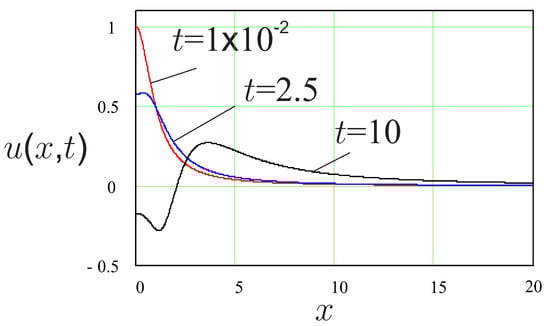
Figure 1. Solution (39) at three time instants for $B=1$, $\alpha =0.1,b=0$, and $\lambda =1\times {10}^{-4}$.

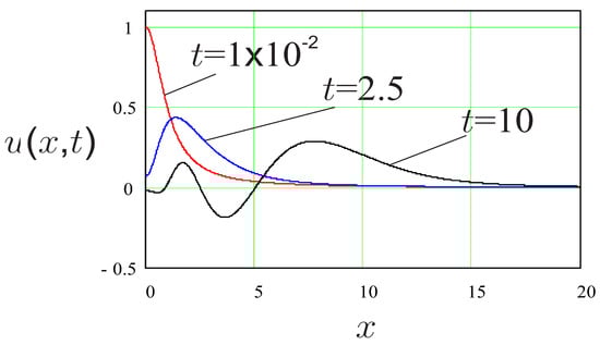
Figure 2. Solution (39) at three time instants for $B=1$, $\alpha =0.1,b=0$, and $\lambda =1$.

(B) As a second example we take $C_1\left(x\right)=\delta \left(x\right)$, $C_2\left(x\right)=0$, for $\alpha =1,b=0.$ Since $\mathcal{F}\left(\delta \right)\left(k\right)=1,$ the Equation (32) becomes

$$u(x,t)=\frac{1}{2\pi }\underset{-\infty }{\overset{\infty }{\int }}cos\left(xk\right)cos\left(B\right|k\left|t\right)dk,$$

(40)

or

$$u(x,t)=\delta (x-Bt).$$

(41)

Equation (41) shows that in this case we have the classical wave equation with the speed of propagation B.

(C) Next, we take $b=1$, $\alpha =0.1$, $\lambda =0.1$, $\beta =0.1$ and $C_1\left(x\right)=\delta \left(x\right)$, $C_2\left(x\right)=0$. By solving (25), we obtain the result shown in Figure 3.

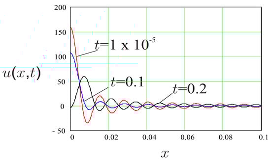
Figure 3. Solution (25) at three time instants for $B=1$, $\alpha =0.1$, $\beta =0.1,b=1$, and $\lambda =0.1$.

(D) Finally we present the solution to (35). We take $B=1$, $C_1\left(x\right)=\delta \left(x\right)$, $C_2\left(x\right)=0$, for $\alpha =0.1$, $b=1$, $\lambda =0.1$ $\beta =1.$ Since $\mathcal{F}\left(\delta \right)\left(k\right)=1,$ the Equation (35) becomes

$$\begin{array}{ccc}\hfill u(x,t)& =& \frac{1}{2\pi }\underset{-\infty }{\overset{\infty }{\int }}exp\left(-ixk\right)exp\left(\frac{bt}{2}\right)\left[cos\left(t\sqrt{\mathcal{K}\left(k\right)-\frac{b^2}{4}}\right)\right.\hfill \\ & +& \left.\frac{\frac{b}{2}}{\sqrt{\mathcal{K}\left(k\right)-\frac{b^2}{4}}}sin\left(t\sqrt{\mathcal{K}\left(k\right)-\frac{b^2}{4}}\right)\right]dk.\hfill \end{array}$$

(42)

From the Figure 3 and Figure 4, we conclude that, for the case where other parameters have fixed values, the order of fractional derivative that models external dissipation $\beta$ has small influence on the waves at the beginning of motion. It decreases the amplitude of waves for larger times.

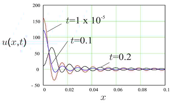
Figure 4. Solution (35) at three time instants for $B=1$, $\alpha =0.1,b=1$, $\beta =1$, and $\lambda =0.1$.

6. Conclusions

In this work, we formulated a new wave equation with non-local action with fractional type of dissipation (24). The solution to the equation is given for several special cases. Our main conclusions are:

1.

We introduced a new measure of deformation, generalizing the classical one-dimensional strain. It is non-local and contains two parameters, $\alpha$ and $\lambda .$ In the special case $\lambda =0$, it is reduced to classical or the strain measure or the generalized strain measure used in [16]. We note that a similar formalism was used in [28] in the context of classical particle mechanics, i.e., a finite number of degrees of freedom.

2.

The solution is a regular distribution. The explicit form of the solution is given with (25)–(27).

3.

The obtained solution shows dissipation in the sense that amplitude is decreasing. However, there is no periodicity/quasiperiodicity of the solution. This is explained by the known property of the fractional derivative: the fractional derivative of a periodic function is not periodic; see [29,30].

References

- Oldham, K.B.; Spanier, J. The Fractional Calculus; Academic Press: New York, NY, USA, 1974. [Google Scholar]
- Miller, K.S.; Ross, B. An Introduction to the Fractional Calculus and Fractional Differential Equations; John Wiley & Sons: New York, NY, USA, 1993. [Google Scholar]
- Gorenflo, R.; Mainardi, F. Fractional Calculus, Integral and Differential Equations of Fractional Order. In Fractional Calculus in Continuum Mechanics; Carpinteri, A., Mainardi, F., Eds.; Springer: Berlin/Heidelberg, Germany, 1977; pp. 223–276. [Google Scholar]
- Samko, S.G.; Kilbas, A.A.; Marichev, O.I. Fractional Integrals and Derivatives; Gordon and Breach: Amsterdam, The Netherlands, 1993. [Google Scholar]
- Podlubny, I. Fractional Differential Equations; Academic Press: San Diego, CA, USA, 1999. [Google Scholar]
- Kilbas, A.A.; Srivastava, H.M.; Trujillo, J.I. Theory and Applications of Fractional Differential Equations; Elsevier: Amsterdam, The Netherlands, 2006. [Google Scholar]
- Lazopulos, K.A. Non-local Continuum Mechanics and Fractional Calculus. Mech. Res. Commun. 2006, 33, 753–757. [Google Scholar] [CrossRef]
- Sandev, T.; Chechkin, A.; Kantz, H.; Metzler, R. Diffusion and Fokker-Planck-Smoluchowski equations with Generalized memory kernel. Fract. Calc. Appl. Anal. 2015, 18, 1006–1038. [Google Scholar] [CrossRef]
- Tarasov, V.E. General Fractional Dynamics. Mathematics 2021, 9, 1464. [Google Scholar] [CrossRef]
- Diethelm, K.; Kiryakova, V.; Luchko, Y.; Tenreiro Machado, J.A.; Tarasov, T.E. Trends, directions for further research, and some open problems of fractional calculus. Nonlinear Dyn. 2022, 107, 3245–3270. [Google Scholar] [CrossRef]
- Tarasov, V.E. General Non-Local Continuum Mechanics: Derivation of Balance Equations. Mathematics 2022, 10, 1427. [Google Scholar] [CrossRef]
- Sandev, T.; Sokolov, I.M.; Metzler, R.; Chechkin, A. Beyond monofractional kinetics. Chaos Solitons Fractals 2017, 102, 210–217. [Google Scholar] [CrossRef]
- Molina-Garcia, D.; Sandev, T.; Safdari, H.; Pagnini, G.; Chechkin, A.; Metzler, R. Crossover from anomalous to normal diffusion: Truncated power-law noise correlations and applications to dynamics in lipid bilayers. New J. Phys. 2018, 20, 103027. [Google Scholar] [CrossRef]
- Atanackovic, T.M.; Guran, A. Theory of Elasticity for Scientists and Engineers; Birkhauser: Boston, MA, USA, 2000. [Google Scholar]
- Tarasov, V.E. General Fractional Calculus in Multi-Dimensional Space: Riesz Form. Mathematics 2023, 11, 1651. [Google Scholar] [CrossRef]
- Atanackovic, T.M.; Stankovic, B. Generalized Wave Equation in Non-local Elasticity. Acta Mech. 2009, 208, 1–10. [Google Scholar] [CrossRef]
- Caputo, M.; Fabrizio, M. A New Definition of Fractional Derivative without Singular Kernel. Prog. Fract. Differ. Appl. 2015, 1, 73–85. [Google Scholar]
- Atanackovic, T.M.; Pilipovic, S.; Zorica, D. Properties of the Caputo–Fabrizio Fractional Derivative and Its Distributional Settings. Fract. Calc. Appl. Anal. 2018, 21, 29–44. [Google Scholar] [CrossRef]
- Gradshteyn, I.S.; Ryzhik, I.M. Table of Integrals, Series and Products; Academic Press: Amsterdam, The Netherlands, 2007. [Google Scholar]
- Stein, E.M. Singular Integrals and Differentiability Properties of Functions; Princeton University Press: Princeton, NJ, USA, 1970. [Google Scholar]
- Schwartz, L. Théorie des Distributions; Hermann: Paris, France, 1957. [Google Scholar]
- Schwartz, L. Méthodes Mathématiques pour les Sciences Physiques; Hermann: Paris, France, 1961. [Google Scholar]
- Szmydt, Z. Fourier Transformation and Linear Differential Equations; Reidel Publishing Company: Dordrecht, The Netherlands, 1977. [Google Scholar]
- Vladimirov, V.S. Generalized Functions in Mathematical Physics; Mir Publishers: Moscow, Russia, 1979. [Google Scholar]
- Titchmarsh, E.C. Introduction to the Theory of Fourier Integrals; Clarendon Press: Oxford, UK, 1948. [Google Scholar]
- Baclic, B.S.; Atanackovic, T.M. Stability and Creep of a Fractional Derivative Order Viscoelastic Rod. Bulletin 2000, 25, 115–131. [Google Scholar]
- Magnus, W.; Oberhettinger, F. Formeln und Sätze für die Speziellen Funktionen der Mathematischen Physik; Springer: Berlin/Heidelberg, Germany, 1948. [Google Scholar]
- Klimek, M. Fractional Sequential Mechanics—Models with Symmetric Fractional Derivative. Czechoslov. J. Phys. 2001, 51, 1348–1354. [Google Scholar] [CrossRef]
- Area, I.; Losada, J.; Nieto, J.J. On Fractional Derivatives and Primitives of Periodic Functions. Abstr. Appl. Anal. 2014, 2014, 392598. [Google Scholar]
- Garrappa, R.; Kaslik, E.; Popolizio, M. Evaluation of Fractional Integrals and Derivatives of Elementary Functions: Overview and Tutorial. Mathematics 2019, 7, 407. [Google Scholar]
Disclaimer/Publisher’s Note: The statements, opinions and data contained in all publications are solely those of the individual author(s) and contributor(s) and not of MDPI and/or the editor(s). MDPI and/or the editor(s) disclaim responsibility for any injury to people or property resulting from any ideas, methods, instructions or products referred to in the content. |
© 2023 by the authors. Licensee MDPI, Basel, Switzerland. This article is an open access article distributed under the terms and conditions of the Creative Commons Attribution (CC BY) license (https://creativecommons.org/licenses/by/4.0/).