Start-Up Strategy-Based Resilience Optimization of Onsite Monitoring Systems Containing Multifunctional Sensors

Abstract

In nonrepairable multifunctional systems, the lost function of a component can be restored by the same function from another component; therefore, the activation mechanism of redundant functions illustrates that multifunctional systems have resilience features. This study evaluates the resilience of multifunctional systems and analyzes the properties of system resilience first. To determine the optimal start-up strategy, a resilience-oriented start-up strategy optimization model for onsite monitoring systems (OMSs) is established to maximize system resilience under a limited budget. In this study, real-time reliability is regarded as the system performance to evaluate the system resilience, and a two-stage local search based genetic algorithm (TLSGA) is proposed to solve the resilience optimization problem. The results of our numerical experiments show that the TLSGA can more effectively solve the problems for OMSs, with high function failure rates and low component failure rates compared with classical genetic algorithms under 48 systems. Moreover, the optimal combinations of unmanned aerial vehicles (UAVs) for an OMS under a limited budget shows that UAVs with a higher carrying capacity should be given priority for selection. Therefore, this study provides an effective solution for determining the optimal start-up strategy to maximize the resilience of OMSs, which is beneficial for OMS configuration.

1. Introduction

As technology continues to advance, a component can perform multiple functions, and such components usually have a basic function with one or more additional capabilities. Multifunctional systems are widely used in various engineering fields, including power transmission [1], energy storage and conversion [2,3], 3D manufacturing [4,5], and water quality monitoring [6]. A multifunctional system containing multifunctional components aims to provide several functions required to complete one task; however, all the functions or components are nonrepairable. If a function in a component is lost, the corresponding functions of other components are activated and connected to the system to ensure the required functions. Multifunctional systems do not fail until a function is completely lost; thus, the multifunctional system can resist external interference. Some researchers have focused on the reliability analysis of multifunctional systems. Moreover, researchers are focusing on the ability of complex systems to resist external disruptive events, among which resilience is an important indicator for evaluating system performance. Many complex systems should consider resilience because system suspension will cause substantial economic losses, especially in major engineering systems such as interdependent infrastructures [7], transportation systems [8], power systems [9], and container ports [10], oil and gas supply chain management [11], logistics systems [12], international trade [13], the large-scale optimization of damage functions [14], UAV networks [15], and epidemic vaccination [16]. The automatic replenishment of failed functions in a multiple functional system indicates the resistance ability of the system; therefore, it is necessary to analyze the resilience of multifunctional systems with multifunctional components.

Resilience has become an important consideration in system design, evaluation, and optimization [17]. Many scholars have focused on evaluating and enhancing system resilience to resist external risks. Several evaluation methods are available to quantify the resistance of complex systems. In a smart grid, the resilience of a power system can be quantitatively measured by the total load of the service [18]. Wu et al. [19] reviewed the optimization methods for cyber-physical power system resilience from three perspectives. For a comprehensive performance management system, a DEA framework of data envelopment analysis for a dynamic network was proposed to assess the performance of a supply chain based on resilience over time [20]. A figure of merit-based method was developed to determine system resilience according to the constituent elements of the tradespace processes that are currently used to select the preferred design alternatives [21]. Under the resilience evaluation framework, a sequential Monte Carlo simulation method was proposed to integrate the real-time weather condition [22]. Considering the influence of hurricane wind, a fully probabilistic and analytical measurement framework has been proposed to evaluate the resilience of a linear power distribution system [23]. A full probabilistic and analytical measurement framework has been designed to assess the resilience of linear power distribution systems affected by hurricane wind [24]. A twofold procedure based on data envelopment analysis and the Tobit model has been proposed to evaluate the effect of resilience conditions on the energy sector [25]. Supply chain resilience is an increasing concern for diverse types of disturbances in quantitative methods, including analysis frameworks [26]. Moreover, some scholars have focused on enhancing system resilience to reduce the degradation process. The upgradation and repair of network poles have been developed as hardening strategies to improve the resilience of the distribution network [9]. Improving network resilience is often associated with reducing vulnerability by using a tri-level optimization method [27]. To maximize infrastructure resilience, limited budgets and resources must be wisely allocated to components to reduce the consequences of low-probability high-impact events [28]. The optimal defense strategy of reconfigurable systems was obtained using a genetic algorithm to maximize the defensive capability for resisting external risks [29]. Resilience enhancement strategies can be obtained using a fast non-dominated sorting genetic algorithm to minimize costs and maximize system resilience [30]. The location selection strategy of emergency rescue facilities in a multimodal transport network was obtained using a cooperative coverage model to improve system resilience [31]. In summary, considerable work has been devoted to quantifying and describing resilience from different perspectives; however, there are no universal metrics for evaluating the resilience of different systems under different hazards. Resilience optimization is one of the most popular topics in the field of system performance optimization under external risks. Based on the research reported in the literature, a gap analysis for system resilience is summarized in

Table 1. Research gap analysis for system resilience.

References	System Performance Indexes	Optimization Algorithms
[18]	Integrated response	✗
[19]	The disaster probability, caused damage, and response measures in grid	Generation decomposition algorithm
[20]	Failure time and recovery probability	Segmentation algorithm
[21]	Scale function	✗
[22]	Recovery curve	Network topology optimization
[23]	Fuzzy logical relationship	✗
[24]	Probability for decision making	Monte Carlo simulation algorithm
[25]	Energy efficiency and energy security	✗
[26]	Analog derivation	✗
[27]	Failure time and recovery rate	✗
[28]	Examination time and functional level	✗
[29]	defensive capability	Genetic algorithm
[30]	Examination time and functional level	✗
[31]	Cooperative coverage model	✗

from the perspectives of the system performance index and optimization algorithms. Different indices were selected to evaluate system performance; however, system reliability was not selected as the performance index. Many studies have focused on resilience evaluation instead of resilience optimization; however, the optimization algorithms consist of some classical algorithms, including genetic algorithms and Monte Carlo simulations. Therefore, it is necessary to develop a new system performance index and effective optimization algorithms.

Many scholars have analyzed and evaluated the performance of multifunctional systems. The reliability of a one-shot system containing multifunctional components was analyzed using an integrated analysis of component reliability, function reliability, and the interrelationship among the components and functions [32]. A new goal-oriented method was presented to analyze the reliability of repairable systems with multifunctional components [33]. The functional resonance analysis method was used to determine the risk of multifunctional flood defenses [34]. A reliability evaluation methodology was presented for multifunctional processes that use a reliability-centered maintenance approach and modify general power generation functions in a large-scale manufacturing environment [35]. The reliability of a multifunctional inverter was analyzed by considering actual industrial reactive power curve injection [36]. The safety of multifunctional flood-defined systems has been evaluated based on the failure probability of multiple reinforcement strategies [37]. A continuous-time Markov chain method was developed to evaluate the time-dependent reliability of a multifunctional system using a known start-up strategy [38]. The reliability of multifunctional complex systems has been presented using hazard rate matrix and Markovian approximation [39]. In addition, some researchers have studied the performance optimization of multifunctional systems. A multifunctional automatized forging station with a supervisory system for process and production management was developed in [40] to produce high-quality and low-price forgings. A reliability optimization model for multifunctional systems with multistate units was built to minimize system cost in [41]. By considering multifunctional maintenance windows, a state-based maintenance decision problem was introduced but the authors of [42] to ensure a flexible balance of inspection and spare parts. A validated thermodynamic model was established to determine the optimal energy and exergy configurations of a two-stage multifunctional hybrid open absorption system [43]. An effective metaheuristic algorithm model was established to reduce the total cost and solve the problem of preventive maintenance scheduling based on production planning and reliability [44]. A sequential quadratic programming algorithm was designed to solve the reliability optimization problem of multistage supply chains [45]. In summary, many scholars have focused on the reliability evaluation of multifunctional systems; however, few scholars have focused on the resilience evaluation and optimization of multifunctional systems.

The aim of this study is to evaluate the real-time reliability of a multifunctional system for quantifying system resilience. Unlike in the reported study, the real-time reliability analysis of a multifunctional system must consider when and how the start-up strategy changes before a specific point in time, making the problem more complicated. Once a component fails, all of its functions can no longer be used. Determining the reliability of components or functions according to their lifetime distributions is difficult because of the dependency between a component and its functions. The evaluation of system resilience mainly depends on changes in the actual system performance over time, which is one of the most important processes for calculating system resilience. Obtaining an optimal start-up strategy for multifunctional systems is another challenge.

The remainder of this paper is organized as follows: Section 2 introduces the definition, assumptions, and resilience evaluation of a nonrepairable multifunctional system containing multifunctional components. Section 3 describes the resilience-oriented start-up strategy optimization of multifunctional systems. In Section 4, a two-stage local search-based genetic algorithm is developed to solve the optimization problem. Section 5 presents two experiments to illustrate the performance of the proposed algorithm and optimal start-up strategy for onsite monitoring systems under a limited budget. Finally, concluding remarks and directions for future research are provided in Section 6.

2. Resilience Analysis of Onsite Monitoring Systems

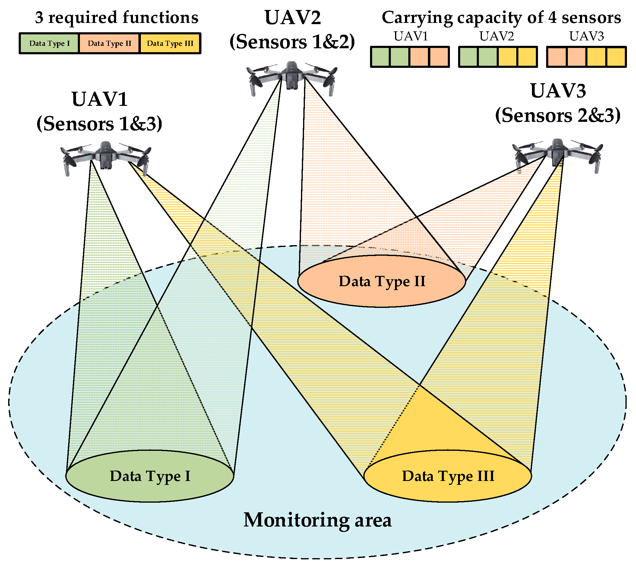
2.1. Onsite Monitoring Systems Containing Multifunctional Sensors

An onsite monitoring system (OMS) consists of multifunctional sensors, and they are used to complete one task with several required monitoring functions. In onsite monitoring systems, the required functions are satisfied by combining the multifunctional sensors with components. Maintenance activities cannot be implemented when the system is operating, and the lost function of one component can be supplemented with the same function of the other components. The system fails when a required function is lost and cannot be complemented by other components. The structure of an onsite monitoring system with m components and n required functions is shown in Figure 1.

To better understand the structure, an onsite monitoring system consisting of three UAVs, each carrying two different types of sensors, was introduced to collect onsite information in a certain area, as shown in Figure 2. As shown in Figure 2, each UAV can be regarded as a component with a carrying capacity of four sensors, and this system should collect the three types of data (Types I, II, and III) via the coordination of three UAVs, which are three required functions. If sensor 2 in UAV3 fails, the system loses the required Type II data temporarily. UAV2 can activate carrying sensor 2 to complement the lost function, but the system fails if sensor 2 in UAV2 fails. The system fails if no functions that can complement the required functions are available from the other components.

The start-up strategy includes the initial selection of functions and the redundancy level, which is the number of functions for all components. An available start-up strategy should select a subset of functions from the components to satisfy the required functions. Moreover, the complementary mechanism of the OMS is important for guaranteeing the required functions. Therefore, it is necessary to determine the optimal start-up strategy to extend system survival time.

2.2. Assumptions of OMSs

Some reasonable assumptions that can be made to better evaluate the resilience and start-up strategy optimization of OMSs are summarized as follows:

• In a multifunctional system, the failure of one component does not affect the failure of other components, and a functional failure does not affect the failure of another function in the same component.
• The failure of one component can cause all the functions of this component to be activated regardless of the conditions of the functions.
• If any function of a component is activated, the component is used.
• If no components can provide one of the required functions, the system will fail.
• Considering that sensors are electronic components, the lifetime of the components and their functions follow exponential distributions.
• Information on hazardous events, including the occurrence time and effect of events on components and their functions, is known, and the failure rates of the affected components or functions are larger.

2.3. Resilience Evaluation of OMSs

2.3.1. Real-Time Reliability Analysis of OMSs

To better analyze the real-time reliability of the OMS, changes in the start-up strategy in a specified time duration should be considered; however, it is difficult to enumerate all failure or activation situations. Furthermore, the usage time of components or functions is difficult to determine; therefore, the reliability of components or functions is difficult to obtain. Therefore, a new reliability evaluation method for evaluating the real-time reliability of OMSs should be considered. Considering the lifetime distribution assumptions, the reliability analysis method based on continuous-time Markov chain (CTMC) can be used to determine the state transition process by considering the activation and redundancy level of functions [46]. However, the difficulty of the CTMC model lies in defining the system states and evaluating the transition probability by carrying out the following: (1) Define all the possible system states of the OMSs. (2) Generate all possible states based on the redundancy levels and initial selection of functions. (3) Analyze the transition rates between any two states by considering the failure of components or functions. (4) Calculate system reliability based on the Kolmogorov equations. The detailed process we used is summarized as follows:

• The OMS states were defined. For an OMS containing m components with n required functions, $x_{ij}=1\left(i=1,\cdots ,m;j=1,\cdots ,n\right)$ indicates that function j in component i is initially selected in the start-up strategy; otherwise, $x_{ij}=0$. All possible system states can be represented by a $m\times 2n$ matrix, which includes the initial selection of functions, where the redundancy levels $y_{ij}$ represents the redundancy levels of function j in component i, and $y_{ij}=0$ indicates that the function is lost. Once all elements in column j in the redundancy level part are 0, the system fails because no component can provide the required functions.
• Generate all possible states of the OMS based on a two-step iterative method. Set all the non-zero redundancy levels as one and generate all the system states based on the start-up strategy. Then, consider the combination of real redundancy levels $y_{ij}$ to enumerate all the system states.
• Evaluation of transition rates between different states: To better analyze the transition probability between the different states, the transition rates from state u to state v can be divided into four situations. Situation 1 indicates that state u cannot be transferred to state v by considering the failure of a function or a component, and the transition rates in Situation 1 are 0. Situation 2 indicates that state u can be transferred to state v by considering the failure of a component, and the transition rates are the failure rates of the components. Situation 3 indicates that state u can transfer to state v by considering the failure of a function, and the transition rates are the product of the function’s failure rate and its redundancy levels under state u. Situation 4 indicates that state u can transfer to state v by considering the failure of a component or a function whose redundancy level is 1 for state u, and the transition rates are the sum of the function’s failure rate and the component’s failure rate. In summary, the transition rate $q_{uv}(u\ne v)$ can be determined using the above four situations, and $q_{uu}=-{\displaystyle {\sum }_{u=1,u\ne v}^{N_B}{q}_{uv}},(u=v)$. The transition rate matrix is represented by all $q_{uv}$.
• Calculation of real-time system reliability: Let $E$ contain all the system states, and let $W$ be the set of all the working states. The probability that the system state is u at time t can be denoted as $P_u(t)=\mathrm{Pr}\{X(t)=u\},$$u\in E$ or $P_1(0)=1, P_{u,u\ne 1}(0)=0$. According to the Kolmogorov equations, $P^{\prime }(t)=P(t)Q$, and the probability of all states can be obtained using $P(t)=P(0)e^{Qt}$. Therefore, the system reliability $R(t)$ of OMS can be evaluated by the sum of the probabilities that the system is in the working states, as shown in Equation (1).

  $$R(t)={\displaystyle {\sum }_{v\in W}{P}_v(t)},$$

  (1)

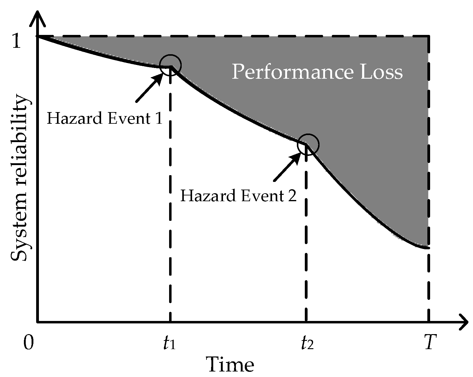
2.3.2. Resilience Definition for OMSs

Under hazardous events, system resilience can be defined as the ability of a system to resist the external environment and reduce system performance losses [47]. When hazardous events occur, system performance will degrade over time. The classical evaluation method for system resilience is equal to the ratio of the area enclosed by the real performance curve and time axis to the area enclosed by the ideal performance and time axes [48], as shown in Figure 3.

If system reliability is selected as the index of system performance, the resilience of OMSs can be evaluated by the ratio of the area enclosed by the real performance curve and time axis $S_{real}$ to the area enclosed by the ideal performance curve and time axis $S_{ideal}$. $S_{real}$ is equal to ${\displaystyle {\int }_0^{T}R(t)}dt$, and $S_{ideal}$ is rectangular. Therefore, in $f_{SR}(T)$, the system resilience at time T can be calculated as

$$f_{SR}(T)=\frac{S_{real}}{S_{ideal}}=\frac{{\displaystyle {\int }_0^{T}R(t)}dt}{T}$$

(2)

${\displaystyle {\int }_0^{T}R(t)}dt$ can be directly evaluated using the differential element method, though this can be time-consuming. With the consideration of evaluating $R(t)$ via CTMC, ${\displaystyle {\int }_0^{T}R(t)}dt$ can be easily calculated using ${\displaystyle {\int }_0^{\infty }R(t)}dt-{\displaystyle {\int }_{t_0}^{\infty }R(t)}dt$, which could reduce time. The detailed derivation of ${\displaystyle {\int }_0^{T}R(t)}dt$, which is the expected residual lifetime after t₀, is listed in Proof of Proposition 1.

Proposition 1. 

According to the assumptions of nonrepairable multifunctional systems, the expected residual lifetime after t0 of this type of system can be calculated using ${\displaystyle {\int }_{t_0}^{\infty }R(t)}dt=-P_W(t_0)B^{-1}{e}_W$.

In this study, we only considered the resistance ability of a multifunctional system under several hazardous events without considering the restoration process because the aforementioned multifunctional systems are nonrepairable. The effects of each hazardous event on the components or functions are known, meaning that the real-time system reliability in the interval $[t_l,t_{l+1}](l=0,1,\cdot \cdot \cdot ,n_d)$ is recorded as $R_{l+1}(t)$, which can be evaluated using Equation (1), where $t_l$ is the occurrence time of the l-th hazardous event, $B_{l+1}$ is the transition matrix between all working states from $t_l$ to $t_{l+1}$, and $e_W$ is a column vector whose elements are one, and the number of elements is equal to the number of working states. The proof of Proposition 1 is as follows.

Proof of Proposition 1. 

The block matrix form of the Kolmogorov equation can be shown as follows:

$$({P^{\prime }}_W(t),{P^{\prime }}_F(t))=(P_W(t),P_F(t))\left(\begin{array}{cc}B& C\\ D& E\end{array}\right)$$

where $P_W(t)=(P_1(t),P_2(t),\cdot \cdot \cdot ,P_N(t))$; $P_F(t)=(P_{N+1}(t),P_{N+2}(t),\cdot \cdot \cdot ,P_{N_0}(t))$; $B$, $C$, $D$, $E$ are the corresponding block matrix forms of transition rates matrix $Q$. For the nonrepairable system, ${P^{\prime }}_W(t)=P_W(t)B$.

To solve this equation quickly, a Laplace transform was introduced to derive the final result. The Laplace form of $P_i(t)$ can be represented as follows:

$$P_i{}^{\ast }(s)={\displaystyle {\int }_0^{\infty }{e}^{-st}{P}_i(t)dt}, s>0, i=1,2,\cdot \cdot \cdot N$$

The Laplace transform of ${P^{\prime }}_W(t)=P_W(t)B$ can be shown as follows:

$${\displaystyle {\int }_0^{\infty }{e}^{-st}{P^{\prime }}_W(t)dt}={\displaystyle {\int }_0^{\infty }{e}^{-st}{P}_W(t)dt}\cdot B, s>0$$

The left side of the above equation can be derived using partial integration as follows:

$$\begin{array}{l}{\displaystyle {\int }_0^{\infty }{e}^{-st}{P^{\prime }}_W(t)dt}=e^{-st}{P}_W(t){|}_0^{\infty }+{\displaystyle {\int }_0^{\infty }{e}^{-st}{P}_W(t)dt}\\ =-P_W(0)+s{\displaystyle {\int }_0^{\infty }{e}^{-st}{P}_W(t)dt}\end{array}$$

Through substituting the result of the two equations above, we can obtain the following:

$$P_W{}^{\ast }(s)={\displaystyle {\int }_0^{\infty }{e}^{-st}{P}_W(t)dt}=P_W(0){(sI-B)}^{-1}$$

The expected lifetime of a nonrepairable system is equal to the meantime to the first failure; thus, ${\displaystyle {\int }_0^{\infty }R(t)dt}=P_W{}^{\ast }(0)=-P_W(0)B^{-1}{e}_W$. $R(t)=P_W(t)e_W$ can be used to obtain ${\displaystyle {\int }_0^{\infty }R(t)dt} = {\displaystyle {\int }_0^{\infty }{P}_W(t)e_{W}dt} = {\displaystyle {\int }_0^{\infty }{P}_W(t)dt}\cdot e_W$. These two equations can get the same results. Therefore, we can conclude that ${\displaystyle {\int }_0^{\infty }{P}_W(t)dt}=-P_W(0)B^{-1}$. □

Based on the above expression, the expected residual lifetime of a nonrepairable system after time t₀ can be calculated as follows:

$$\begin{array}{l}{T}_r={\displaystyle {\int }_{t_0}^{\infty }R(\tau )d\tau } \begin{array}{c}\underset{\_}{\underset{\_}{\mathrm{set} t=\tau -t_0}}\\ \end{array} {\displaystyle {\int }_0^{\infty }R(t+t_0)dt} = {\displaystyle {\int }_0^{\infty }{P}_W(t+t_0)e_{W}dt}\\ ={\displaystyle {\int }_0^{\infty }{P}_W(t+t_0)dt}\cdot e_W={\displaystyle {\int }_0^{\infty }{P}_W(t)e^{B{t}_0}dt}\cdot e_W={\displaystyle {\int }_0^{\infty }{P}_W(t)dt}\cdot e^{B{t}_0}{e}_W\\ \begin{array}{c}\underset{\_}{\underset{\_}{{\displaystyle {\int }_0^{\infty }{P}_W(t)dt}=-P_W(0)B^{-1}}}\\ \end{array}-P_W(0)B^{-1}\cdot e^{B{t}_0}{e}_W=-P_W(t_0)B^{-1}{e}_W\end{array}$$

Proposition 2. 

The expected lifetime of a multifunctional system in the interval [t₀, T], (t₀ = 0), under known $n_d$ hazardous events can be calculated as

$${\displaystyle {\int }_{t_0}^{T}R(t)}dt=P_W(T)B_{n_d+1}{}^{-1}{e}_W-P_W(t_0)B_1{}^{-1}{e}_W+{\displaystyle {\sum }_{l=1}^{n_d}[P_W(t_l)(B_l{}^{-1}-B_{l+1}{}^{-1})e_W]}$$

Proof of Proposition 2. 

The expected lifetime of a nonrepairable onsite monitoring system is the meantime to the first failure. Thus,

$$\begin{array}{l}{\displaystyle {\int }_{t_0}^{T}R(t)}dt={\displaystyle {\sum }_{l=0}^{n_d-1}{\displaystyle {\int }_{t_l}^{t_l+1}{R}_{l+1}(t)}dt}+{\displaystyle {\int }_{t_{n_d}}^{T}R{(t)}_{n_d+1}}dt\\ ={\displaystyle {\sum }_{l=0}^{n_d-1}({\displaystyle {\int }_{t_l}^{\infty }{R}_{l+1}(t)}dt-{\displaystyle {\int }_{t_{l+1}}^{\infty }{R}_{l+1}(t)}dt)}+{\displaystyle {\int }_{t_{n_d}}^{\infty }R{(t)}_{n_d+1}}dt-{\displaystyle {\int }_T^{\infty }R{(t)}_{n_d+1}}dt\\ ={\displaystyle {\sum }_{l=0}^{n_d-1}(-P_W(t_l)B_{l+1}{}^{-1}{e}_W+P_W(t_{l+1})B_{l+1}{}^{-1}{e}_W)}+P_W(t_{n_d})B_{n_d+1}{}^{-1}{e}_W)-P_W(T)B_{n_d+1}{}^{-1}{e}_W\\ =P_W(T)B_{n_d+1}{}^{-1}{e}_W-P_W(t_0)B_1{}^{-1}{e}_W+{\displaystyle {\sum }_{l=1}^{n_d}[P_W(t_l)(B_l{}^{-1}-B_{l+1}{}^{-1})e_W]}\end{array}$$

□

Through combining Equation (2) and Proposition 2, the system resilience at T under $n_d$ hazardous events can be evaluated as follows:

$$f_{SR}(T|n_d)=\frac{P_W(T)B_{n_d+1}{}^{-1}{e}_W-P_W(t_0)B_1{}^{-1}{e}_W+{\displaystyle {\sum }_{l=1}^{n_d}[P_W(t_l)(B_l{}^{-1}-B_{l+1}{}^{-1})e_W]}}{T}$$

(3)

Corollary 1: 

The system resilience at T without hazardous events can be evaluated using $f_{SR}(T|0)=(P_W(T)-P_W(t_0))B_1{}^{-1}{e}_W/T$.

2.4. Resilience Properties of OMSs

2.4.1. Monotonic Analysis of System Resilience

According to the definition of system resilience in Equation (3), the monotonic properties of $f_{SR}(t)$ are summarized in Proposition 3.

Proposition 3. 

If the system reliability of the OMSs $R(t)$ is known, the resilience of the multifunctional system $f_{SR}(t)$ decreases with an increase in t, and the range of $f_{SR}(t)$ is [0, 1].

Proof of Proposition 3. 

(1) Proof of system resilience bounds: In Section 2.3.1, $R(t)$ is a decreasing and continuous function of time. We obtain $\underset{x\to \infty }{\lim }R(t)=0$ and $\underset{x\to \infty }{\lim }R(t)=0$.

Through using $f_{SR}(t)={\displaystyle {\int }_0^{t}R(t)dt}/t$, we can obtain the corresponding limitation of $f_{SR}(t)$.

When $t\to 0$, $\underset{t\to 0}{\lim }{f}_{SR}(t)=\underset{t\to 0}{\lim }\frac{{\displaystyle {\int }_0^{t}R(t)dt}}{t}\underset{\_}{\underset{\_}{L’Hospital’s Rule}}\underset{t\to 0}{\lim }\frac{R(t)}{1}=R(0)=1$.

Because $R(t)$ in the interval $[0,\infty ]$ decreases and bounces, $R(t)$ is integrable, and ${\displaystyle {\int }_0^{t}R(t)dt}$ is finite. Using $t\to \infty$, we can obtain $\underset{t\to \infty }{\lim }{f}_{SR}(t)=0$. Therefore, the lower bounce of $f_{SR}(t)$ is zero, and the upper bounce of $f_{SR}(t)$ is one.

(2) Proof of monotonicity for system resilience: Because $t\ne 0$ when $t>0$, ${f^{\prime }}_{SR}(t)=\left(tR(t)-{\displaystyle {\int }_0^{t}R(t)dt}\right)/t^2$. Set $g(t)=tR(t)-{\displaystyle {\int }_0^{t}R(t)dt}$; the purpose is to determine whether $g(t)$ is less than 0. Moreover, $R(t)$ is differentiable and decreasing so that $R^{\prime }(t)<0$ . We can obtain $g^{\prime }(t)=t{R}^{\prime }(t)<0$, and $g(t)$ will decrease as time increases. At the same time, $g(t){|}_{t=0}=0$. Therefore, $g(t)<0,t>0$. It is easy to find that ${f^{\prime }}_{SR}(t)<0$, which means that $f_{SR}(t)$ decreases with an increase in time t. □

2.4.2. Changes in System Resilience as the Number of Hazardous Events Increases

System resilience is closely related to the number of hazardous events, and it is not difficult to find that the higher the number of hazardous events, the lower the system resilience. To illustrate the effect of the number of hazardous events, the change in system resilience over time with different numbers of hazards when the start-up strategy is fixed is shown in Figure 4. The occurrence times of the hazardous events were $t_1=5$, $t_2=10$, and $t_3=15$.

From Figure 4, it is easy to observe that the system resilience without any hazardous events is much greater than that of a system with hazardous events. At t = 50, the difference between the system resilience at $n_d=0$ and system resilience at $n_d=1$ was approximately 0.12. However, the difference in system resilience narrowed with an increase in hazardous events. For example, the system resilience when $n_d=2$ is very close to that at $n_d=3$, and the difference between them is no greater than 0.0115. Therefore, the system resilience with the same start-up strategy decreases with an increase in the occurrence of hazardous events; however, the difference between system resilience is very close when the number of hazardous events is large.

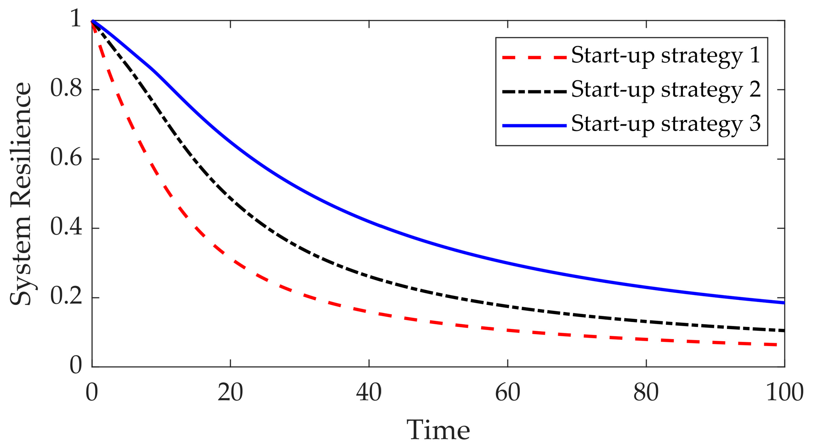
2.4.3. Changes in System Resilience as Start-Up Strategy Adjusts

When the number of hazardous events and parameters of components and functions are determined, different start-up strategies can cause significant differences in system resilience. For a multifunctional system, the number of required functions is 5, and the number of components is 3. From Figure 5, we can observe that the differences between the three different start-up strategies are significant.

From Figure 5, we can see that the system with start-up strategy 3 has the highest resilience over time compared with the systems with the other two start-up strategies. Compared with these three start-up strategies, start-up strategy 3 has two activated components in the initial selection of function, while start-up strategies 1 and 2 have three activated components. We can also conclude that a smaller number of activated components can generate higher system resilience when the redundancy levels of the functions are similar [37]. To maximize the system resilience at a specific time point, the optimal start-up strategy should be determined to increase the ability of a multifunctional system to resist the decrease of system performance.

3. Resilience-Oriented Start-Up Strategy Optimization of Onsite Monitoring Systems

Start-up strategy optimization determines the start-up strategy for maximizing the resilience of an onsite monitoring system with known hazardous events. The occurrence time and effects of all of the hazardous events are known.

The objective is to maximize system resilience under a limited budget. The decision variables are the start-up strategy, including the initial selection of functions and the redundancy levels of all functions. The mathematical model was established as follows:

$$\max f_{SR}(X,Y|n_d)$$

(4)

s.t.

$$x_{ij}=\{0,1\},(i=1,2,\cdot \cdot \cdot ,m; j=1,2,\cdot \cdot \cdot ,n)$$

(5)

$${\displaystyle {\sum }_{i=1}^m{x}_{ij}}=1,(j=1,2,\cdot \cdot \cdot ,n)$$

(6)

$$y_{ij}\ge x_{ij},y_{ij}\in Z,(i=1,2,\cdot \cdot \cdot ,m; j=1,2,\cdot \cdot \cdot ,n)$$

(7)

$${\displaystyle {\sum }_{j=1}^n{y}_{ij}}\le n_0,(i=1,2,\cdot \cdot \cdot ,m)$$

(8)

$$m{C}_0+{\displaystyle {\sum }_{j=1}^n{\displaystyle {\sum }_{i=1}^m{c}_{ij}{y}_{ij}}}\le C_{\max }$$

(9)

Constraints (5) and (6) are related to the initial selection of the start-up strategy. In Constraint (5), $x_{ij}=1 (i=1,\cdot \cdot \cdot ,m;j=1,\cdot \cdot \cdot ,n)$ indicates that function j in component i is initially selected; otherwise, $x_{ij}=0$. Constraint (6) indicates that each function must be selected from a single component. Constraints (7) and (8) define the limits of the redundancy levels of functions. Constraint (7) shows that $x_{ij}$ must equal zero if $y_{ij}=0$ (i.e., component i does not have function j), and the redundancy levels must be integers. Constraint (8) describes the carrying capacity of each UAV, which means that the total redundancy levels of each UAV should be less than or equal to $n_0$. Constraint (9) illustrates the cost limitation of the UAVs, and the corresponding redundancy of functions is supposed to be less than the budget $C_{\max }$, where $C_0$ is the unit cost of the UAV.

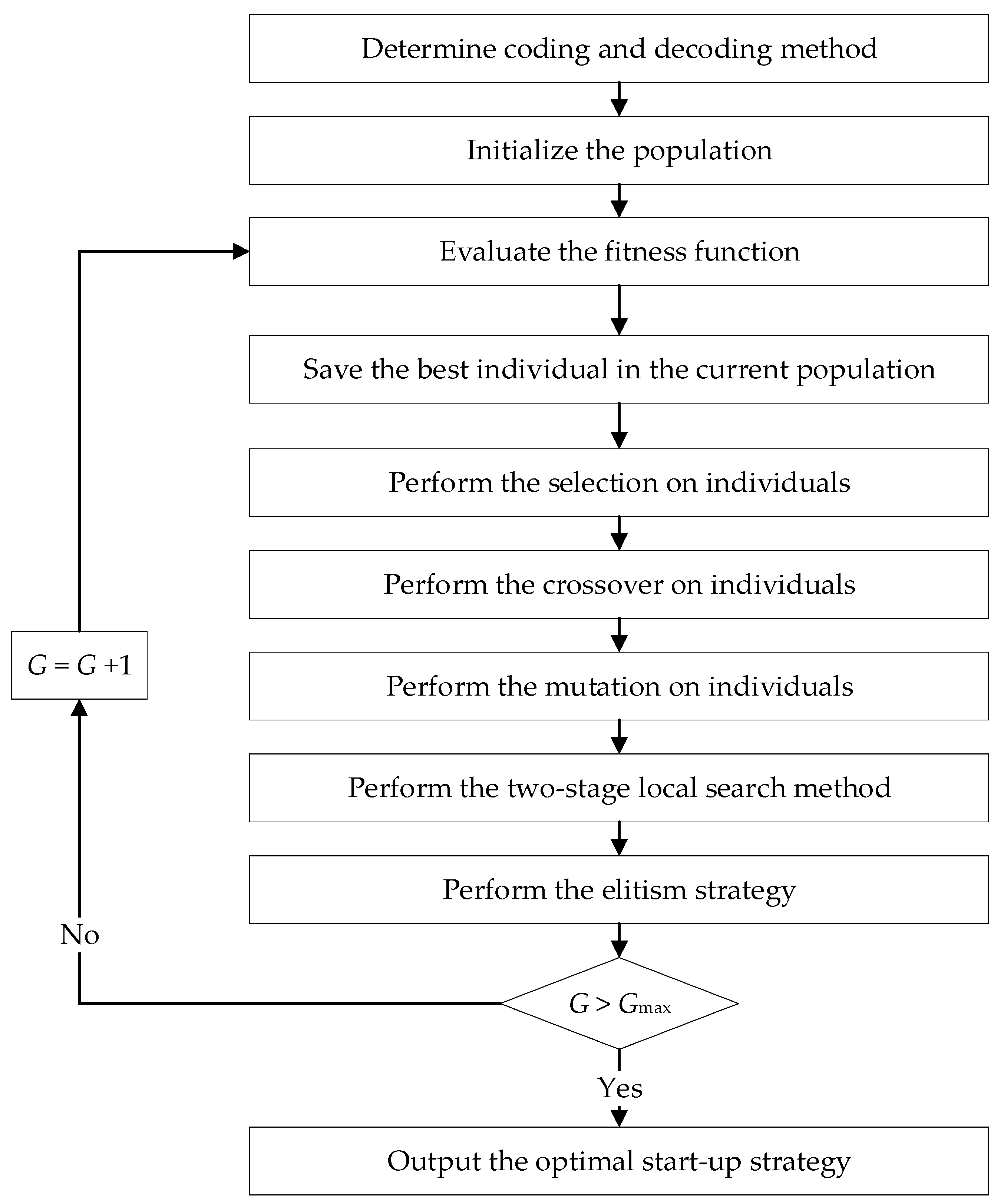
4. Solving Algorithm

A genetic algorithm (GA) is a remarkable meta-heuristic algorithm that utilizes the survival of the fittest idea to determine the optimal solution [49]. GA has good global search ability because it can dynamically increase the diversity of population via crossover and mutation; however, GA has weak local search ability [50]. Considering the advantages of importance measures on the local search ability, a two-stage local search was developed to enhance the local search ability of the GA [51]. To determine the optimal start-up strategy model for onsite monitoring systems, a two-stage local search-based genetic algorithm (TLSGA) was developed by adding a two-stage local search process to improve the GA.

4.1. Two-Stage Local Search Method

Considering the advantage of the importance measure for finding the weakest links of a system, it can potentially cost-effectively improve the system performance by increasing the maintenance resources for the components with the highest importance [52]. The local search method is used to update the start-up strategy by adjusting the start-up strategy to maximize system resilience, which involves two stages: the first stage is the redundancy adjustment of a component based on the redundancy importance measure; the second stage is the adjustment of the initial selection for a function. By considering the constraints of the initial selection and redundancy level, the detailed ideas of the local search method can be summarized as follows:

(1) To adjust the redundancy level, each component has a limit of carrying functions, which is less than n₀; a component is selected by removing and adding one redundant function to maximize the improvement in system resilience under the unchanged carrying capacity of the component. The detailed redundancy adjustment process of component i* is as follows:

• Choose the function $j_1{}^{*}=\arg \min \left\{j\right|f_{SR}(T|X,Y_i^j)-f_{SR}(T|X,Y_i^j-1),j=1,\cdot \cdot \cdot ,n\}$ with minimum resilience reduction when removing its redundant function by one.
• Choose the function $j_2{}^{*}=\arg \max \left\{j\right|f_{SR}(T|X,Y_i^j+1)-f_{SR}(T|X,Y_i^{j_1{}^{*}}),j=1,\cdot \cdot \cdot ,n\}$ with maximum resilience increase when adding its redundant function by one.
• Determine the component i^* with the maximum improvement of system resilience by $i^{*}=\arg \max \left\{j\right|f_{SR}(T|X,Y_i^{j_2{}^{*}}+1)-f_{SR}(T|X,Y_i^{j_1{}^{*}}-1),i=1,\cdot \cdot \cdot ,m\}$.

(2) To adjust the initial selection of functions, the same function from other components should be considered to replace the current function; therefore, the component with the maximum improvement in system resilience should be selected to provide the same function. Thus, the detailed process of start-up strategy function adjustment can be summarized as follows:

• Find the component with the maximum improvement in system resilience by adjusting the start-up strategy of function j according to $i_s{}^{*}(j)=\arg \max \left\{i\right|f_{SR}(T|X_i^{j^{*}}-1,Y)-f_{SR}(T|X_i^j+1,Y),j=1,\cdot \cdot \cdot ,n\}$.
• Determine the function of the component by maximizing the improvement in system resilience by $j_s{}^{*}=\arg \max \left\{j\right|i_s^{*}(j),j=1,\cdot \cdot \cdot ,n\}$.

In summary, we should choose the optimal component redundancy and start-up strategy adjustment to maximize the improvement in system resilience.

4.2. TLSGA Procedures

The TLSGA takes advantage of the better global search ability of the GA and better local search ability of the two-stage local search method. The procedures of the TLSGA are similar to those of the GA, which is a classical meta-heuristic algorithm with a standard process that includes initialization, selection, crossover, and mutation. The real number encoding method is used to represent the start-up strategy in the TLSGA, which is an $m\times 2n$ matrix. The difference between the TLSGA and GA is that the local search process is added after the mutation process in the TLSGA. A flow chart of the TLSGA procedures is shown in Figure 6.

5. Numerical Experiments

5.1. Performance Comparison between TLSGA and GA

5.1.1. Experimental Design

The performance of the TLSGA and GA in different systems was compared in an experiment (Experiment 1). For Experiment 1, the high and low failure rates of components and their functions were categorized into four groups: low ${\lambda }_f$ and low ${\lambda }_c$, high ${\lambda }_f$ and low ${\lambda }_c$, low ${\lambda }_f$ and high ${\lambda }_c$, and high ${\lambda }_f$ and high ${\lambda }_c$. For each group, there are 12 systems, the symbols of which are listed in

Table 2. The symbols of the 12 systems with different parameters.

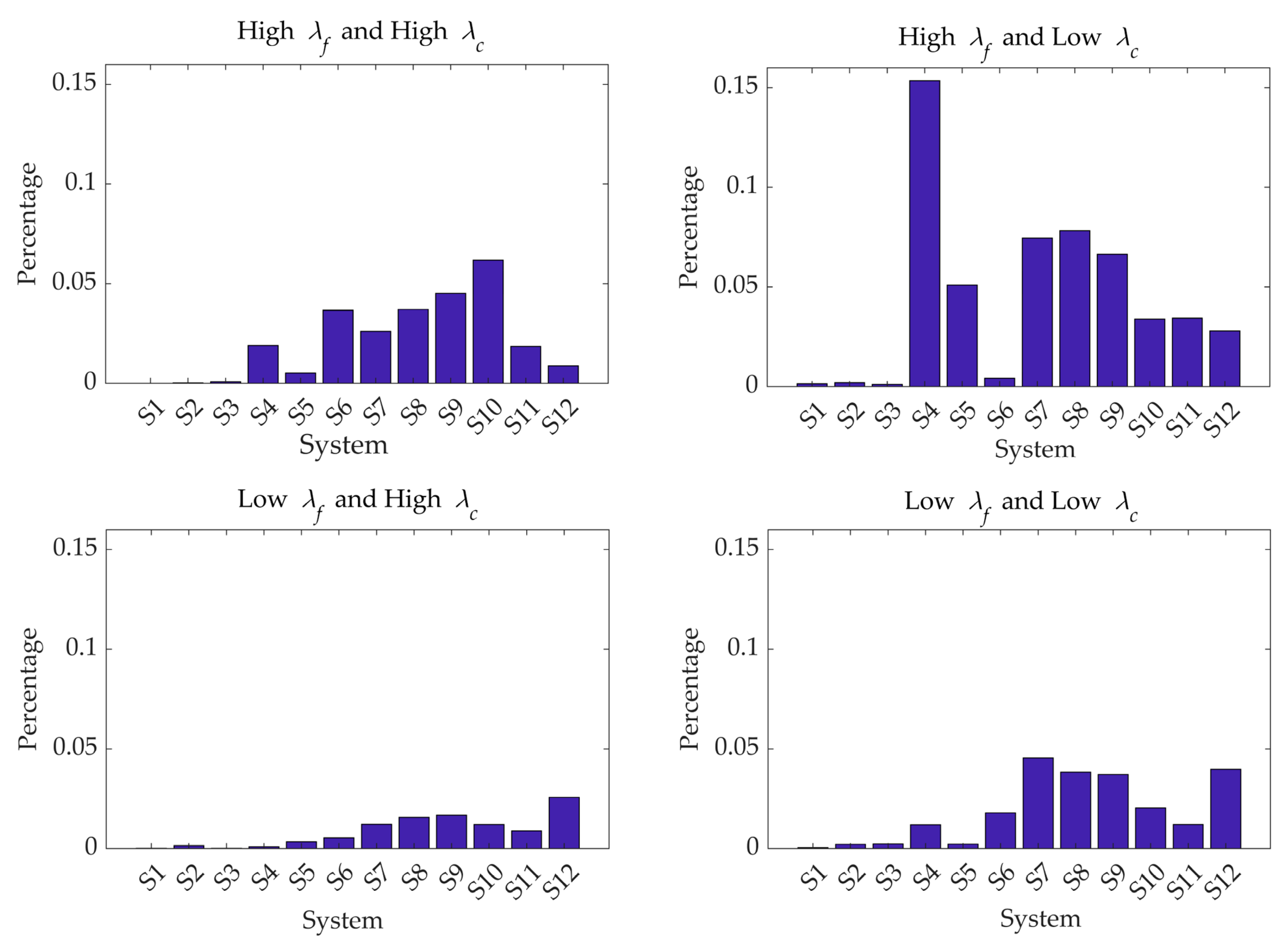
System #	Component Number m	The Number of Required System Functions n	Carrying Capacity of Component n0	The Number of Hazardous Events nd
1	2	3	4	0
2	2	3	4	1
3	2	3	4	2
4	3	3	2	0
5	3	3	2	1
6	3	3	2	2
7	3	3	4	0
8	3	3	4	1
9	3	3	4	2
10	3	5	4	0
11	3	5	4	1
12	3	5	4	2

; each system has a different component number m, required number of system functions n, carrying capacity of component n₀, and number of hazardous events n_d.

The UAV fails more easily than the sensors; therefore, the failure rate of the components is higher than that of the functions. A low ${\lambda }_c$ is randomly selected from the interval [0.1, 0.3], and a high ${\lambda }_c$ ${\lambda }_c$ is randomly selected from [0.8, 1]; a low ${\lambda }_f$ ${\lambda }_c$ is randomly selected from [0.01, 0.02], and a high ${\lambda }_f$ ${\lambda }_c$ is randomly selected from [0.08, 0.1]. Hazardous events occur at the 3rd and 7th hour, respectively. Moreover, the parameters of the TLSGA and GA included a population size of 100, a maximum number of generations of 200, a crossover probability of 0.9, and a mutation probability of 0.1. For each system, the TLSGA and GA were employed 50 times.

Two indices were used to analyze the performance of the TLSGA and GA: the improved number (IN) and the mean ratio of system resilience (MRSR). IN is used to count the number for which the result of the TLSGA is not less than that of the GA, and MRSR is the average ratio of the system resilience obtained by the TLSGA to that obtained by the GA. A higher IN or higher MRSR indicates that the performance of the TLSGA is better than that of the GA. Moreover, the applicability of the TLSGA can be analyzed using the average percentage improvement in system resilience. The improvement percentage $P_{isr}$ can be evaluated using Equation (10) as follows:

$$P_{isr}=\frac{R_{TLSGA}-R_{GA}}{R_{GA}}$$

(10)

where $R_{TLSGA}$ is the system resilience obtained by the TLSGA, and $R_{GA}$ is the system resilience obtained by the GA.

5.1.2. Experimental Results

The experimental results are listed in

Table 3. The simulation results of Experiment 1.

System #	$\mathbf{High} {\mathit{\lambda }}_{\mathit{f}}$$\mathbf{and} \mathbf{High} {\mathit{\lambda }}_{\mathit{c}}$		$\mathbf{High} {\mathit{\lambda }}_{\mathit{f}}$$\mathbf{and} \mathbf{Low} {\mathit{\lambda }}_{\mathit{c}}$		$\mathbf{Low} {\mathit{\lambda }}_{\mathit{f}}$$\mathbf{and} \mathbf{High} {\mathit{\lambda }}_{\mathit{c}}$		$\mathbf{Low} {\mathit{\lambda }}_{\mathit{f}}$$\mathbf{and} \mathbf{Low} {\mathit{\lambda }}_{\mathit{c}}$
	IN	MRSR	IN	MRSR	IN	MRSR	IN	MRSR
S1	50	1.0001	50	1.0015	50	1.0001	50	1.0005
S2	50	1.0002	50	1.0022	50	1.0015	50	1.0023
S3	50	1.0009	50	1.0012	50	1.0002	50	1.0027
S4	50	1.0194	50	1.1854	50	1.0009	49	1.0140
S5	50	1.0064	50	1.0539	49	1.0035	50	1.0023
S6	49	1.0434	50	1.0045	50	1.0070	50	1.0192
S7	47	1.0274	46	1.0868	41	1.0127	49	1.0491
S8	47	1.0398	47	1.0923	47	1.0163	49	1.0409
S9	49	1.0489	48	1.0754	48	1.0175	48	1.0400
S10	49	1.0736	49	1.0362	47	1.0145	44	1.0228
S11	45	1.0211	46	1.0381	48	1.0106	47	1.0135
S12	48	1.0093	46	1.0297	47	1.0321	45	1.0463

. Table 3 shows that IN decreased with an increase in the scale of the systems. The INs are almost 50 for systems S1–S6 in these four groups, but the INs become smaller for systems S7–S12. The lowest IN was 45, which means that at least 90% of the results obtained by the TLSGA were better than those of the GA. By analyzing the MRSR, we found that the performance of the TLSGA and the GA were similar when the system scale is small, as is the case in S1, S2, and S3. However, the MRSR in S1, S2, and S3 is smaller than that in the other systems, which means that the performance of the TLSGA improves with an increase in n. Therefore, the performance of the TLSGA is generally better than that of the GA.

The average percentage improvement in the resilience of each system can be used to discuss the performance of the TLSGA in four different groups to analyze its applicability. The average improvement percentages are shown in Figure 7. Although the improvement percentage is lower in systems with low ${\lambda }_f$ and high ${\lambda }_c$, the performance of the TLSGA is better than that of the GA because the percentage is positive. A positive percentage indicates that the TLSGA can achieve a higher system resilience than the GA. From Figure 7, it can be seen that the TLSGA is more suitable for solving systems with high ${\lambda }_f$ and low ${\lambda }_c$ because the improvement percentage is much higher than that of the other three groups. Regarding the improvement percentage, the TLSGA and the GA in systems with high ${\lambda }_f$ and ${\lambda }_c$ have similar performances in systems with low ${\lambda }_f$ and ${\lambda }_c$. Therefore, the TLSGA can solve the optimization model and obtain a better solution than the GA, especially for systems with high ${\lambda }_f$ and low ${\lambda }_c$.

5.2. Numerical Case for Onsite Monitoring Systems

The optimal design of the onsite monitoring system determines the optimal combinations of the number of UAVs m and the carrying capacity of a UAV n₀ to maximize the system resilience. Once the number of required system functions and the maximum budget are determined, the optimal system resilience with different m and n₀ can be obtained using the TLSGA. The hazardous event occurs on the third hour, and its effect was recorded. The maximum budget was USD 55,000, the unit price of the sensors was USD 1000, and the unit price of the UAV depended on the carrying capacity of the sensors, which was equal to 1000n₀. The maximum system resilience at t = 10 h was obtained by the TLSGA. Therefore, the optimal system resilience with different combinations of m and n₀ can be obtained using the TLSGA.

From Figure 8, we can see that the maximum system resilience is 0.2003 when t = 10 h, and the optimal combination occurs when the number of UAVs is three and the carrying capacity of each UAV is five. When the maximum budget is USD 55,000, the system resilience increases with an increase in the carrying capacity when m = 3 and 4. Similarly, system resilience increases with an increase in the number of UAVs when n₀ = 2 and 3 because the carrying capacity of each UAS is small. With an increase in the number of UAs, the redundancy of the entire system will increase; thus, the system resilience will increase. However, the system resilience decreases when m is 5 and n₀ is greater than 3. To some extent, the sensors in the UAV may have lower redundancy when they carry more types of sensors, which may decrease the system resilience. From the results of Experiment 2, the maximum budget cannot provide sufficient sensors with an increase in m and n₀; therefore, some UAVs may carry sensors whose amount does not reach the maximum carrying capability. From our experimental results, we can observe that the number of UAVs cannot be too large because of the limited budget, and a UAV with a higher carrying capacity should be selected first. Moreover, the TLSGA can determine the optimal configuration of OMSs under a limited budget by considering the combination of the number of UAVs and carrying capability to maximize system resilience. The TLSGA can be applied to integer program problems under nonlinear constraints in practical engineering by adjusting the initialization method and fitness function.

6. Conclusions

This study evaluated the resilience of OMSs by considering real-time reliability and system performance, and the novelty of this study lies in the fact that we evaluated real-time system reliability based on CIMC. A TLSGA was developed to effectively solve the resilience-oriented start-up strategy optimization problem, especially for systems with high ${\lambda }_f$ and low ${\lambda }_c$. Moreover, under a limited budget, a UAV with a higher carrying capacity should be selected first to determine the optimal combinations of m and n₀. The proposed method focuses on exponential distribution and known risk situations. In Future, more research works should focus on complex and uncertain risk situations and other types of distributions of components and their functions.

References

- Chen, Z.; Li, X.; Li, H. Multifunction Transformer With Adjustable Magnetic Stage Based on Nanocomposite Semihard Magnets. IEEE Trans. Ind. Electron. 2020, 67, 4226–4234. [Google Scholar] [CrossRef]
- Adam, T.J.; Liao, G.; Petersen, J.; Geier, S.; Finke, B.; Wierach, P.; Kwade, A.; Wiedemann, M. Multifunctional Composites for Future Energy Storage in Aerospace Structures. Energies 2018, 11, 335. [Google Scholar] [CrossRef]
- Liu, Y.-L.; Shi, Y.; Yang, C.-L. Two-Dimensional MoSSe/g-GeC van Der Waals Heterostructure as Promising Multifunctional System for Solar Energy Conversion. Appl. Surf. Sci. 2021, 545, 148952. [Google Scholar] [CrossRef]
- Guo, X.; Xue, Z.; Zhang, Y. Manufacturing of 3D multifunctional microelectronic devices: Challenges and opportunities. NPG Asia Mater. 2019, 11, 29. [Google Scholar] [CrossRef]
- Yang, Y.; Vervust, T.; Dunphy, S.; Van Put, S.; Vandecasteele, B.; Dhaenens, K.; Degrendele, L.; Mader, L.; De Vriese, L.; Martens, T.; et al. 3D Multifunctional Composites Based on Large-Area Stretchable Circuit with Thermoforming Technology. Adv. Electron. Mater. 2018, 4, 1800071. [Google Scholar] [CrossRef]
- Akhter, F.; Siddiquei, H.R.; Alahi, M.E.E.; Jayasundera, K.P.; Mukhopadhyay, S.C. An IoT-Enabled Portable Water Quality Monitoring System With MWCNT/PDMS Multifunctional Sensor for Agricultural Applications. IEEE Internet Things J. 2022, 9, 14307–14316. [Google Scholar] [CrossRef]
- Nipa, T.J.; Kermanshachi, S. Resilience measurement in highway and roadway infrastructures: Experts’ perspectives. Prog. Disaster Sci. 2022, 14, 100230. [Google Scholar] [CrossRef]
- Twumasi-Boakye, R.; Sobanjo, J.O. A Computational Approach for Evaluating Post-Disaster Transportation Network Resili-ence. Sustain. Resilient Infrastruct. 2021, 6, 235–251. [Google Scholar] [CrossRef]
- Tari, A.N.; Sepasian, M.S.; Kenari, M.T. Resilience assessment and improvement of distribution networks against extreme weather events. Int. J. Electr. Power Energy Syst. 2021, 125, 106414. [Google Scholar] [CrossRef]
- Almutairi, A.; Collier, Z.A.; Hendrickson, D.; Palma-Oliveira, J.M.; Polmateer, T.L.; Lambert, J.H. Stakeholder Mapping and Disruption Scenarios with Application to Resilience of a Container Port. Reliab. Eng. Syst. Saf. 2019, 182, 219–232. [Google Scholar] [CrossRef]
- Khezeli, M.; Najafi, E.; Molana, M.H.; Seidi, M. A sustainable and resilient supply chain (RS-SCM) by using synchronisation and load-sharing approach: Application in the oil and gas refinery. Int. J. Syst. Sci.-Oper. Logist. 2023, 10, 2198055. [Google Scholar] [CrossRef]
- Nezhadroshan, A.M.; Fathollahi-Fard, A.M.; Hajiaghaei-Keshteli, M. A scenario-based possibilistic-stochastic programming approach to address resilient humanitarian logistics considering travel time and resilience levels of facilities. Int. J. Syst. Sci.-Oper. Logist. 2020, 8, 321–347. [Google Scholar] [CrossRef]
- Sayarshad, H.R. International Trade Resilience with Applied Welfare Economics: An Analysis on Personal Protective Equip-ment. Int. J. Syst. Sci.-Oper. 2023, 10, 2199131. [Google Scholar] [CrossRef]
- Li, X.-Q.; Song, L.-K.; Choy, Y.-S.; Bai, G.-C. Multivariate ensembles-based hierarchical linkage strategy for system reliability evaluation of aeroengine cooling blades. Aerosp. Sci. Technol. 2023, 138, 108325. [Google Scholar] [CrossRef]
- Lamri, M.A.; Abilov, A.; Vasiliev, D.; Kaisina, I.; Nistyuk, A. Application Layer ARQ Algorithm for Real-Time Multi-Source Data Streaming in UAV Networks. Sensors 2021, 21, 5763. [Google Scholar] [CrossRef]
- Meng, X.; Cai, Z.; Si, S.; Duan, D. Analysis of epidemic vaccination strategies on heterogeneous networks: Based on SEIRV model and evolutionary game. Appl. Math. Comput. 2021, 403, 126172. [Google Scholar] [CrossRef]
- Zuo, M. System reliability and system resilience. Front. Eng. Manag. 2021, 8, 615–619. [Google Scholar] [CrossRef]
- Wu, G.; Li, Z.S. Cyber—Physical Power System (CPPS): A review on measures and optimization methods of system resilience. Front. Eng. Manag. 2021, 8, 503–518. [Google Scholar] [CrossRef]
- Huang, G.; Wang, J.; Chen, C.; Qi, J.; Guo, C. Integration of Preventive and Emergency Responses for Power Grid Resilience Enhancement. IEEE Trans. Power Syst. 2017, 32, 4451–4463. [Google Scholar] [CrossRef]
- Ramezankhani, M.; Torabi, S.A.; Vahidi, F. Supply chain performance measurement and evaluation: A mixed sustainability and resilience approach. Comput. Ind. Eng. 2018, 126, 531–548. [Google Scholar] [CrossRef]
- Ferris, T.L.J. A Resilience Measure to Guide System Design and Management. IEEE Syst. J. 2019, 13, 3708–3715. [Google Scholar] [CrossRef]
- Li, Y.; Xie, K.; Wang, L.; Xiang, Y. Exploiting network topology optimization and demand side management to improve bulk power system resilience under windstorms. Electr. Power Syst. Res. 2019, 171, 127–140. [Google Scholar] [CrossRef]
- Kadan, M.; Özkan, G.; Özdemir, M.H. Resilience Measurement System: A Fuzzy Approach. In Intelligent and Fuzzy Techniques: Smart and Innovative Solutions; Springer: Berlin/Heidelberg, Germany, 2021; Volume 1197, pp. 576–581. [Google Scholar]
- Sharma, P.; Chen, Z. Probabilistic Resilience Measurement for Rural Electric Distribution System Affected by Hurricane Events. ASCE-ASME J. Risk Uncertain. Eng. Syst. Part A Civ. Eng. 2020, 6, 04020021. [Google Scholar] [CrossRef]
- Aldieri, L.; Gatto, A.; Vinci, C.P. Evaluation of energy resilience and adaptation policies: An energy efficiency analysis. Energy Policy 2021, 157, 112505. [Google Scholar] [CrossRef]
- Ribeiro, J.P.; Barbosa-Povoa, A. Supply Chain Resilience: Definitions and quantitative modelling approaches—A literature review. Comput. Ind. Eng. 2018, 115, 109–122. [Google Scholar] [CrossRef]
- Ghorbani-Renani, N.; González, A.D.; Barker, K.; Morshedlou, N. Protection-Interdiction-Restoration: Tri-Level Optimization for En-hancing Interdependent Network Resilience. Reliab. Eng. Syst. Saf. 2020, 199, 106907. [Google Scholar] [CrossRef]
- Najarian, M.; Lim, G.J. Optimizing infrastructure resilience under budgetary constraint. Reliab. Eng. Syst. Saf. 2020, 198, 106801. [Google Scholar] [CrossRef]
- Zhao, J.; Zhang, Z.; Xu, T.; Cao, X.; Wang, Q.; Cai, Z. Defensive strategy optimization of consecutive-k-out-of-n systems under deterministic external risks. Eksploat. Niezawodn.–Maint. Reliab. 2022, 24, 306–316. [Google Scholar] [CrossRef]
- Liu, X.; Fang, Y.-P.; Zio, E. A Hierarchical Resilience Enhancement Framework for Interdependent Critical Infrastructures. Reliab. Eng. Syst. Saf. 2021, 215, 107868. [Google Scholar] [CrossRef]
- Guo, J.; Du, Q.; He, Z. A method to improve the resilience of multimodal transport network: Location selection strategy of emergency rescue facilities. Comput. Ind. Eng. 2021, 161, 107678. [Google Scholar] [CrossRef]
- Xu, Y.; Liao, H. Reliability Analysis and Redundancy Allocation for a One-Shot System Containing Multifunctional Compo-nents. IEEE Trans. Rel. 2016, 65, 1045–1057. [Google Scholar] [CrossRef]
- Yi, X.-J.; Shi, J.; Mu, H.-N.; Dong, H.-P.; Zhang, Z. Reliability Analysis of Repairable System with Multiple-Input and Multi-Function Component Based on Goal-Oriented Methodology. ASCE-ASME J. Risk Uncert. Engrg. Sys. Part B Mech. Engrg. 2017, 3, 014501. [Google Scholar] [CrossRef]
- Anvarifar, F.; Voorendt, M.Z.; Zevenbergen, C.; Thissen, W. An application of the Functional Resonance Analysis Method (FRAM) to risk analysis of multifunctional flood defences in the Netherlands. Reliab. Eng. Syst. Saf. 2017, 158, 130–141. [Google Scholar] [CrossRef]
- López-Campos, M.; Kristjanpoller, F.; Viveros, P.; Pascual, R. Reliability Assessment Methodology for Massive Manufacturing Using Multi-Function Equipment. Complexity 2018, 2018, 1–8. [Google Scholar] [CrossRef]
- Callegari, J.; Silva, M.; de Barros, R.; Brito, E.; Cupertino, A.; Pereira, H. Lifetime evaluation of three-phase multifunctional PV inverters with reactive power compensation. Electr. Power Syst. Res. 2019, 175, 105873. [Google Scholar] [CrossRef]
- Marijnissen, R.; Kok, M.; Kroeze, C.; van Loon-Steensma, J. Re-evaluating safety risks of multifunctional dikes with a probabilistic risk framework. Nat. Hazards Earth Syst. Sci. 2019, 19, 737–756. [Google Scholar] [CrossRef]
- Zhao, J.; Si, S.; Cai, Z.; Liao, H. Time-dependent Reliability Analysis of a Nonrepairable Multifunctional System Containing Multifunctional Components. In Proceedings of the 2020 Asia-Pacific International Symposium on Advanced Reliability and Maintenance Modeling (APARM), Vancouver, BC, Canada, 20–23 August 2020; pp. 1–6. [Google Scholar] [CrossRef]
- Zhou, D.; Sun, C.; Du, Y.-M.; Guan, X. Degradation and reliability of multi-function systems using the hazard rate matrix and Markovian approximation. Reliab. Eng. Syst. Saf. 2020, 218, 108166. [Google Scholar] [CrossRef]
- Hawryluk, M.; Kaszuba, M.; Gronostajski, Z.; Sadowski, P. Systems of supervision and analysis of industrial forging processes. Eksploat. Niezawodn.-Maint. Reliab. 2016, 18, 315–324. [Google Scholar] [CrossRef]
- Yi, X.; Dhillon, B.S.; Shi, J.; Mu, H.; Hou, P. Reliability Optimization Allocation Method for Multifunction Systems with Mul-tistate Units Based on Goal-Oriented Methodology. ASCE-ASME J. Risk Uncert. Engrg. Sys. Part B Mech. Engrg. 2017, 3, 041010. [Google Scholar] [CrossRef]
- Zhang, Z.; Yang, L. State-Based Opportunistic Maintenance With Multifunctional Maintenance Windows. IEEE Trans. Reliab. 2021, 70, 1481–1494. [Google Scholar] [CrossRef]
- Shahzad, M.K.; Ding, Y.; Xuan, Y.; Gao, N.; Chen, G. Performance analysis of a novel double stage multifunctional open absorption heat pump system: An industrial moist flue gas heat recovery application. Energy Convers. Manag. 2022, 254, 115224. [Google Scholar] [CrossRef]
- Gharoun, H.; Hamid, M.; Torabi, S.A. An Integrated Approach to Joint Production Planning and Reliability-Based Multi-Level Preventive Maintenance Scheduling Optimization for a Deteriorating System Considering Due-Date Satisfaction. Int. J. Syst. Sci.-Oper. 2022, 9, 489–511. [Google Scholar]
- Gharaei, A.; Amjadian, A.; Shavandi, A. An integrated reliable four-level supply chain with multi-stage products under shortage and stochastic constraints. Int. J. Syst. Sci.-Oper. Logist. 2023, 10, 1958023. [Google Scholar] [CrossRef]
- Zhao, J.-B.; Hou, P.-Y.; Cai, Z.-Q.; Li, Y.; Guo, P. Research of Mission Success Importance for a Multi-State Repairable k-out-of-n System. Adv. Mech. Eng. 2018, 10, 168781401876220. [Google Scholar] [CrossRef]
- Yodo, N.; Wang, P.; Rafi, M. Enabling Resilience of Complex Engineered Systems Using Control Theory. IEEE Trans. Reliab. 2018, 67, 53–65. [Google Scholar] [CrossRef]
- Nan, C.; Sansavini, G. A quantitative method for assessing resilience of interdependent infrastructures. Reliab. Eng. Syst. Saf. 2017, 157, 35–53. [Google Scholar] [CrossRef]
- Holland, J.H. Genetic algorithms. Sci. Am. 1992, 267, 66–73. [Google Scholar] [CrossRef]
- Katoch, S.; Chauhan, S.S.; Kumar, V. A review on genetic algorithm: Past, present, and future. Multimed. Tools Appl. 2021, 80, 8091–8126. [Google Scholar] [CrossRef]
- Javidi, M.M.; Kermani, F.Z. Utilizing the advantages of both global and local search strategies for finding a small subset of features in a two-stage method. Appl. Intell. 2018, 48, 3502–3522. [Google Scholar] [CrossRef]
- Si, S.; Zhao, J.; Cai, Z.; Dui, H. Recent advances in system reliability optimization driven by importance measures. Front. Eng. Manag. 2020, 7, 335–358. [Google Scholar] [CrossRef]