Abstract
The study of fuzzy geometry and its different components has grown in recent years, establishing the formal foundations for its development. This paper is devoted to addressing some metric relations in the fuzzy right triangle; in particular, a version of the Pythagorean theorem and geometric mean theorem are provided in analytical fuzzy geometry. The main results show, under certain conditions of the fuzzy vertices, a subset relation between the fuzzy distances associated with the fuzzy right triangle, which is very similar to the classical statements of the Pythagorean theorem and the geometric mean in Euclidean geometry.
MSC:
94D05; 03E72
1. Introduction
The aim of this paper is to study some metric relations in a fuzzy right triangle following the ideas from [1,2]. Particularly, we provide a version of the altitude and Pythagorean theorems in analytical fuzzy plane geometry.
Set theory was born, as a separate mathematical discipline, with the work developed by Georg Cantor in 1874 [3]. The elegance of this theory led current mathematics to consider it an essential pillar of the foundations of this science. The idea of using sets to formalize mathematics is to define all mathematical objects as sets: numbers, functions, algebras, geometric figures, etc. However, the strict dichotomy of belonging or not belonging to a set can make certain tasks or decisions complicated. In particular, determining what belongs or does not belong to a set that uses unclear, fuzzy, or vague terms, such as determining the objects in the set of beautiful colors, can be difficult. Sometimes, drastic decisions are made based on these classifications, which are not always easy to make.
In the mid-1960s, Lotfi A. Zadeh introduced the notions of fuzzy sets in his famous paper, entitled “Fuzzy sets” [4]. His aim was to represent, in a mathematical way, the uncertainty generated by the vague definition of some sets, using values between 0 and 1 to represent how much an object belongs to a set (with 1 meaning that it certainly belongs, 0 meaning that it certainly does not belong, and intermediate values meaning that it partially belongs). Formally, a fuzzy set consists of ordered pairs such that
where is the membership function of the set and (see [4,5]).
Fuzzy set theory has advanced in various ways and across many disciplines. Applications of this theory are found, for example, in artificial intelligence, computer science, decision theory, control theory, logic, management science, and robotics. See, for instance [6,7,8,9,10,11].
Ideas about fuzzy geometric notions have been proposed by many researchers, providing notions of point, line, angle, plane, area, perimeter, and shapes; see, for example, the references [12,13,14,15,16,17,18,19]. However, only Buckley and Eslami, in the papers [1,2], gave some ideas on the construction and representation of basic fuzzy geometric entities in a mathematical framework. Subsequently, Ghosh and Chakraborty, based on the works [1,2], provided different contributions to analytical fuzzy plane geometry (see, for instance, [20,21]). Moreover, Ghosh et al. also contributed to analytical fuzzy space geometry (see [22,23]), as did Qiu and Zhang in [24].
The aim of this paper is to study some metric relations in a fuzzy right triangle following the ideas from [1,2]. Particularly, we use the definitions of fuzzy distance, fuzzy point, and fuzzy triangle provided in the paper [1]. Since the fuzzy distance between two fuzzy points is a fuzzy number (see Section 2.2), the metric relations that are stated are naturally inclusion relations. Specifically, we provide a version of the altitude and Pythagorean theorems considering fuzzy points that define cones with circular bases in fuzzy geometry. It is worth noting that the sense of the inclusion relation changes, as it depends on the radii associated with the circular bases (see Theorems 1 and 2), or there may not even be a relation of inclusion (see Example 3). In the case where all radii are congruent, inclusion is only possible in each statement; more accurately, we state that , and , where , and are the fuzzy distances associated to a fuzzy right triangle (see Corollaries 1 and 2, respectively).
To achieve the aforementioned objective, we present a general characterization of the -cut set of fuzzy distance denoted by between two fuzzy points. Furthermore, we show that if two fuzzy points, and , define a cone with circular bases of radii and , respectively, then , where a is the Euclidean distance between the points in that have membership function equal to 1 (for more details, see Section 3). We utilize some definitions and results of convex sets, since the -cut set of a fuzzy point is a compact and convex subset of (Definition 7).
The paper is organized as follows: Section 2.1 contains generalities about fuzzy sets, fuzzy numbers, and the -cut set. Section 2.2 recalls the basic definitions of fuzzy geometry, which are fuzzy point, fuzzy line segment, fuzzy distance, and fuzzy triangle.
Section 3 provides, in a general way, the -cut set of fuzzy distance . In Section 4, we deal with two metric relations in the fuzzy right triangle. Specifically, a version of the geometric mean and Pythagorean theorems is provided in fuzzy geometry. To state the geometric mean theorem, it is necessary to introduce the altitude definition of a fuzzy triangle. Section 5 is devoted to illustrating some examples from Section 4. Finally, in Section 6, some comments and conclusions are presented.
2. Preliminaries
In this section, some definitions and results that come from [1,2,4,5] are reviewed.
2.1. Fuzzy Set and Fuzzy Number
The following are definitions of fuzzy sets and fuzzy numbers.
Definition 1
(Fuzzy set [4]). Let X be a classical set. Then, the set of order pairs
is called a fuzzy set on X. The evaluation function is called membership function or grade of membership of x in .
Definition 2
(-Cut set [25]). For a fuzzy set , its α-cut is denoted by and is defined by
Notice that the -cut set is not a fuzzy set.
To represent the construction of the membership function of a fuzzy set , we adopt the notation , which means .
Proposition 1.
For all , the following apply:
- 1.
- if and only if .
- 2.
- if and only if .
The proof of the above proposition can be found in [21].
Definition 3.
The support of a fuzzy set , denoted by , is defined as
Definition 4
(Core [5]). The core of a fuzzy set , denoted by , is defined as . When the core has at least one element, we have a normal fuzzy set.
Definition 5
(Convex fuzzy set [5]). A fuzzy set is convex if all its α-cuts are convex.
Definition 6
(Fuzzy number [5]). A fuzzy set is a fuzzy number if and only if is convex, is normalized, and has bounded support, and its α-cuts are closed intervals for .
Since the -cuts of fuzzy numbers are always closed and bounded intervals, the arithmetic of fuzzy numbers is defined in terms of their -cuts (for more details, see [5]).
Let us consider intervals and , subsets of . Then, the following apply:
- Addition
- Multiplicationwhere and
2.2. Fuzzy Geometry
The following are definitions of fuzzy geometry and come from [1,2].
Definition 7
(Fuzzy point [1]). A fuzzy point at , denoted by , is defined by its membership function, which satisfies the following conditions:
- 1.
- is upper semi-continuous;
- 2.
- ;
- 3.
- is a compact and convex subset of .
If there is no confusion, fuzzy point is simply denoted by .
From the above definition, we can see that can be considered a surface on , which is the graph of (see Example 1).
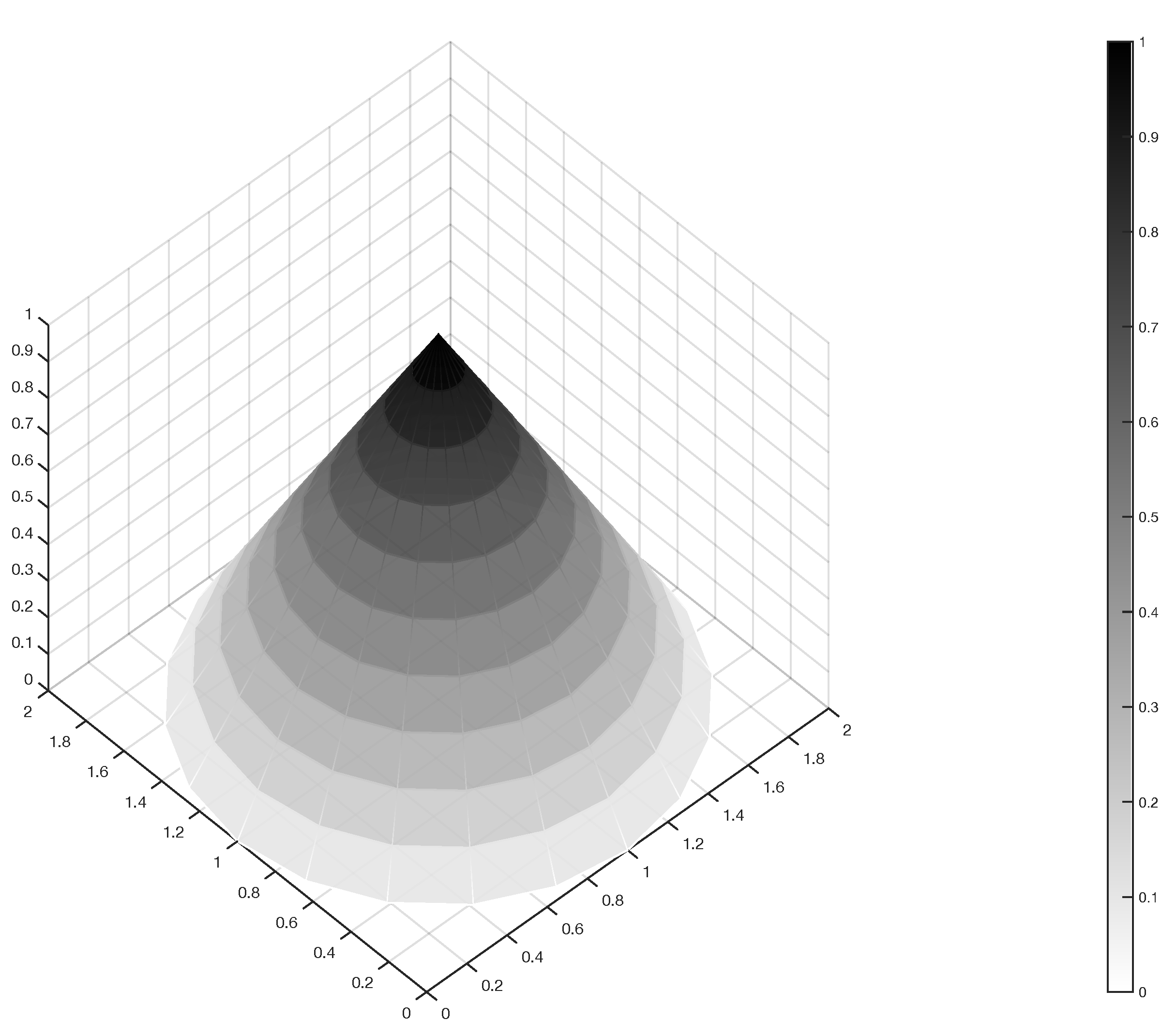
Example 1.

Figure 1.
Fuzzy point at .
We denote by the usual Euclidean distance metric on .
Definition 8
(Fuzzy distance [1]). Fuzzy distance between two fuzzy points and is defined by its membership function
The authors in [1] show that is a fuzzy number in .
Remark 1.
The previous definition of fuzzy distance is different from the one in [20]. The support of the fuzzy distance proposed in [20] must always be a subset of the fuzzy distance introduced by Bluckley and Eslami in [1]. However, their cores are identical.
In order to define a fuzzy line segment, we denote by the line segment defined by points X and Y belonging to .
Definition 9
(Fuzzy line segment [1]). Fuzzy line segment between two fuzzy points and is defined by its membership function
If there is no confusion, fuzzy line segment is simply denoted by .
Let be three distinct points in that define a triangle, and let be a fuzzy point at , with .
Definition 10
(Fuzzy triangle [1]). Let be fuzzy segments between and , and , and , respectively. Then, the fuzzy set
is a fuzzy triangle, and it is defined by its membership function
Moreover, we say that the fuzzy triangle is strongly non-degenerate if , , are pairwise disjoint. Finally, we say that is a fuzzy right triangle at if and only if core is a right triangle at .
Throughout this paper, the phrase fuzzy right triangle always means “strongly non-degenerate fuzzy right triangle”.
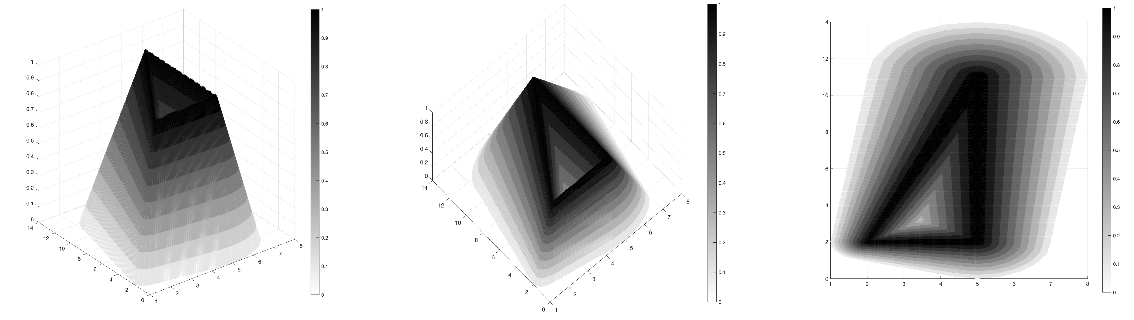
Example 2.

Let , and be three fuzzy points defined by their membership functions
respectively. Then, fuzzy triangle is a fuzzy right triangle at . We can see the graph of in Figure 2.
Figure 2.
On the left and at the center, two views of the fuzzy triangle. On the right side, a level set of .
3. -Cut Set of Fuzzy Distance
In this section, we will define the -cut set of fuzzy distance between two fuzzy points. For the latter, we will set some notations, and since each -cut set of a fuzzy point is a compact and convex subset of (Definition 7), we will recall a few elements about convex sets. The description of will be helpful in Section 4, where the main results are presented.
We consider endowed with the classical Euclidean distance, denoted by . The distance, denoted by d, between a point y and a set is defined as . Furthermore, the distance between two sets X and Y, denoted by , is defined as . Finally, the boundary of a subset is denoted by .
Remark 2.
In general, does not satisfy the positiveness property, and it does not satisfy the triangle inequality property either; hence, is not really a distance function; however, it is usually called distance. For more details, see [26].
The following propositions can be found in [27] or [28].
Proposition 2.
Let X be a closed non-empty and convex subset of . For each , there exists a unique point that minimizes the distance from y, i.e., .
Proposition 3.
Let X be a closed non-empty and convex subset of . If , then .
From the previous propositions, .
Let be two distinct points in , and let and be two fuzzy points at and , respectively, such that and are pairwise disjoint and .
Let us remember that Definition 8 determines the fuzzy distance between fuzzy points and as
where
where denotes the boundary of , with .
In what follows, we will show that and can be expressed in terms of .
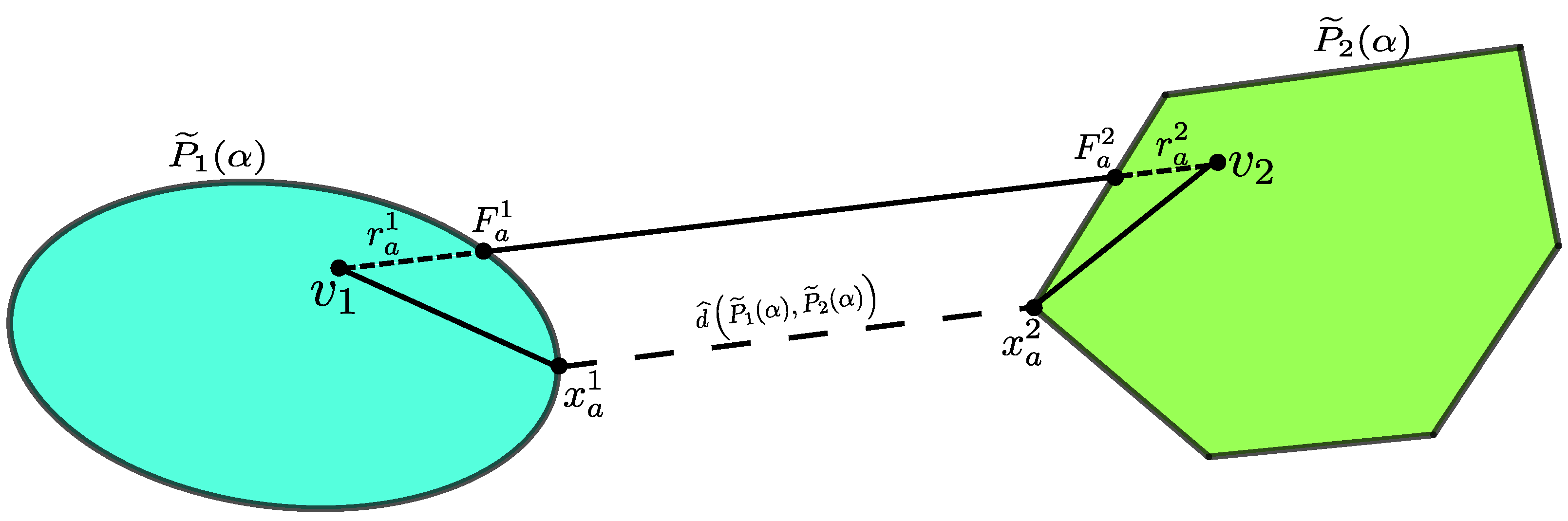
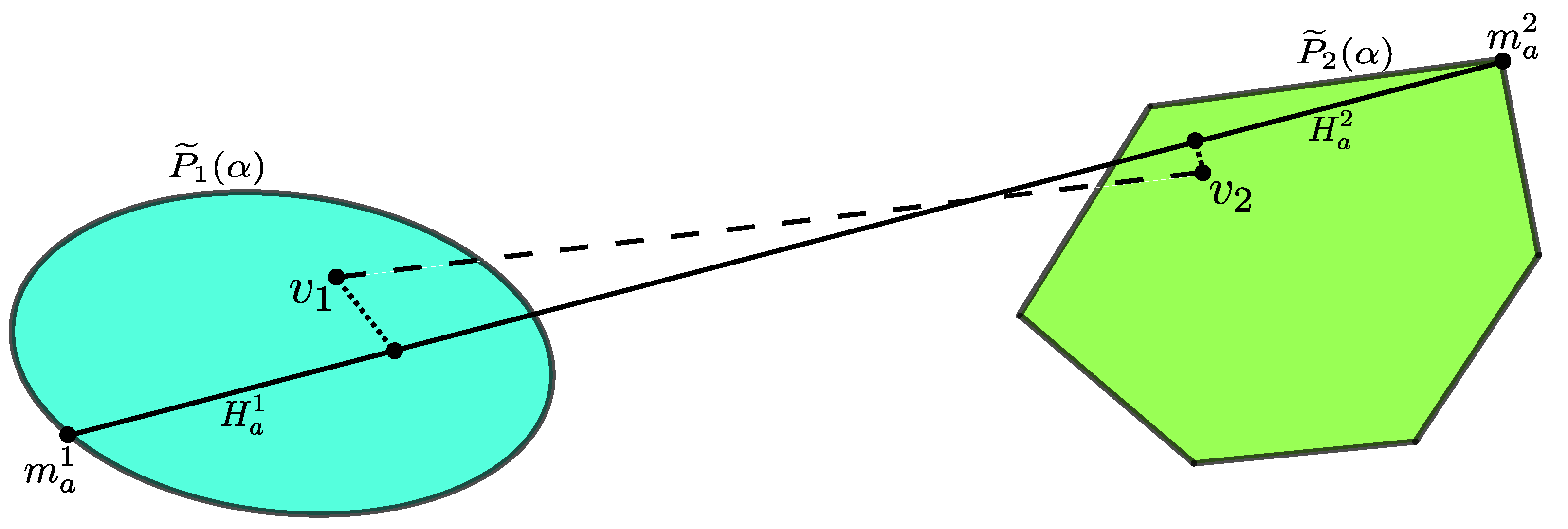
We denote by and the points belonging to and , respectively, such that , and by and the points of intersection between line segment and the boundaries of and , respectively, that is,
Finally, we set
For all of the above, see Figure 3.
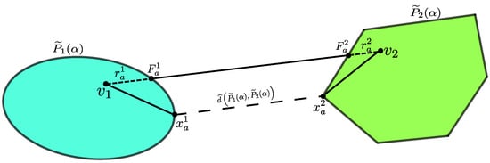
Figure 3.
Minimum distance between the -cut sets of fuzzy points and .
Remark 3.
It is clear that , , , , , and depend on α. However, to simplify the notation, we simply denote them without the α reference.
Since and are the points that define the distance between and , ; hence, we can identify two points, denoted by and , between and onto , such that (see Figure 4). We set and . Then, we have
hence, we obtain
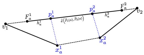
Figure 4.
Projection of and onto .
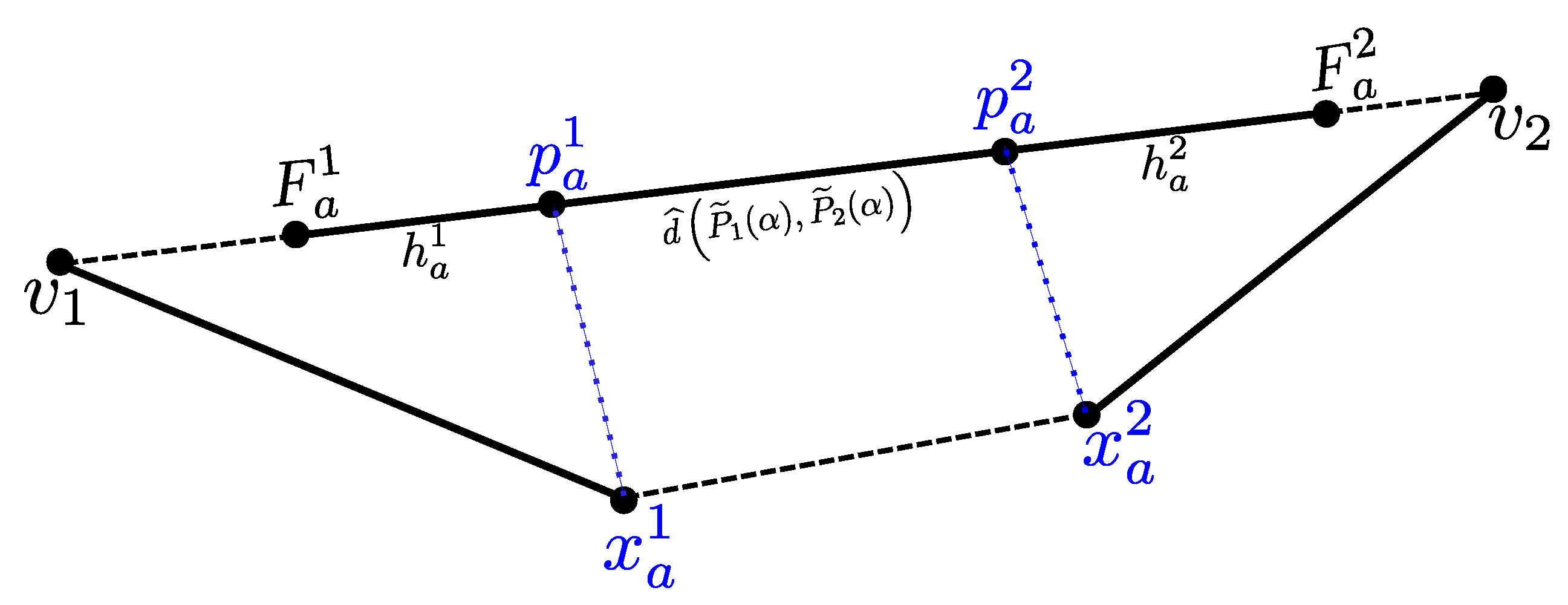
On the other hand, we denote by and the points that define the maximum distance between and . Since , we can identify two points, denoted by and , between and such that . We set and (see Figure 5). Then,
Therefore, by Equations (1) and (2), we have
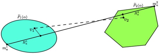
Figure 5.
Projection of and onto the segment defined by and .
Remark 4.
In general, identifying or is a very interesting subject, but it is outside the scope of this paper. However, when the fuzzy points define cones of circular bases, these elements are easy to identify, as we will show in the next section.
4. Some Metric Relations
In this section, we address two metric relations in the fuzzy right triangle, which are the Pythagorean theorem and the geometric mean theorem (also known as Euclidean theorem).
From the above section, it is clear that many different and complicated cases can occur with respect to the form of a 0-cut set of a fuzzy point, so it is necessary to limit ourselves to a few cases. Hereinafter, we consider the following statements: Let be three distinct points in such that , , and . Without losing generality, we assume that .
Let be a fuzzy point at , with , such that they define a fuzzy right triangle at . Moreover, let , , and , i.e., the fuzzy distances associated to each pair of fuzzy points.
We also assume that defines a cone of circular base of radius , with . The membership function for each is given by
with . Moreover,
that is, the boundary of the -cut for is a circle around the core with radius .
Remark 5.
- 1.
- Since is a fuzzy right triangle, , are pairwise disjoint; this implies that , , and .
- 2.
4.1. Fuzzy Pythagorean Theorem
The famous Pythagorean theorem remembered by the majority of students has been extended in different ways and in different geometries. In a very simple way, the law of cosines is one of them. Other versions on different spaces and geometries can be found, for example, in [29,30,31,32].
The above shows that this mathematical result has attracted and still attracts the attention of many researchers who try to generalize or extend the ideas to different geometries or spaces. In this section, we study a version of the Pythagorean theorem in fuzzy geometry considering the conditions of the previous section; that is, we consider fuzzy points defining cones of circular base.
Proposition 4
(Necessary condition). With the previous notation, we have the following:
- 1.
- If , then
- 2.
- If , then
Proof.
From Proposition 4, we have two necessary conditions for two possible inclusions. Then, we can state the following result.
Theorem 1.
With the previous notation, we have the following:
- 1.
- if and only if
- 2.
- if and only if
Proof.
- We can prove item 2 in the same way.
□
Notice that if , then it can only be stated that , since implies , and this is always true in any triangle.
In the case where , we obtain the following result.
Corollary 1.
Let , , and be three fuzzy points defining a fuzzy right triangle at such that , , and . If each is a cone of circular base of radius , then
Proof.
If each is a cone of circular base of radius and they define a fuzzy right triangle, then are pairwise disjoint; this implies that (see Remark 5). On the other hand, by Theorem 1 item 1, if and only if . The latter inequality is always true. The following Lemma is useful to prove it.
Lemma 1.
Let be a right triangle in C, and let , and c be the lengths of the legs and the hypotenuse, respectively, with . If , then .
Proof of Lemma 1.
We assume that . Since , we obtain that . Considering , we obtain . But . In consequence, . □
Then, by Lemma 1, , and since , we conclude that .
4.2. Altitude Theorem or Geometric Mean Theorem
The following metric relation we address is the altitude theorem or geometric mean theorem, also known as Euclidean theorem. For that, it is necessary to define the altitude of a fuzzy triangle. This secondary element of the fuzzy triangle must be a fuzzy segment with one end at one vertex and the other on one side of the triangle. In particular, the ends are vertex and a point on the fuzzy hypotenuse, that is, fuzzy line segment . The following definition is about the containment of a fuzzy point on a fuzzy line segment.
Definition 11
(Containment of a fuzzy point on a fuzzy line segment [1]). We will say that a fuzzy point is contained on a fuzzy line segment if and only if for all .
In [20], a measurement of the degree to which belongs to only when was proposed. Of course, Definition 11 implies the above condition. In Section 6, we provide some comments about the proposal given in [20].
Let be a fuzzy point contained in such that and are disjoint, with We denote by the fuzzy line segment defined by fuzzy points and .
Definition 12.
We will say that is the altitude of fuzzy right triangle from if and only if is perpendicular to .
Other ways of defining altitude can be obtained by following the ideas proposed in [33].
Let be points in such that , , and . Let be a fuzzy point at contained in such that defines a cone of circular base of radius ; and are disjoint, with . Let be the altitude of fuzzy right triangle from , that is, the fuzzy line segment defined by fuzzy points and . Finally, we denote by , , and the fuzzy distances between fuzzy points and , and , and and , respectively.
Proposition 5
(Necessary condition. With the previous notation, we have the following:
- 1.
- If , then
- 2.
- If , then
Proof.
In the same way as in the proof of Proposition 4. □
Another metric relation that relates to the altitude theorem is that the squared measure of a leg is the product between the measure of the leg projection and the hypotenuse measure, i.e., and . We also provide a necessary condition about these relations.
Proposition 6
(Necessary condition. With the previous notation, we have the following:
- 1.
- If , then
- 2.
- If , then
- 3.
- If , then
- 4.
- If , then
Proof.
In the same way as in the proof of Proposition 4. □
As in the previous subsection, the subset relation may vary, giving rise to two cases in each statement. The following result summarizes this fact.
Theorem 2.
With the previous notation, we have the following:
- 1.
- if and only if
- 2.
- if and only if
- 3.
- if and only if
- 4.
- if and only if
- 5.
- if and only if
- 6.
- if and only if
Proof.
In the same way as in the proof of Theorem 1, but using Proposition 5 or Proposition 6. □
Let us notice that if , then we only have a possibility of inclusion in each classical statement. The following result summarizes this fact.
Corollary 2.
Let , , and be three fuzzy points defining a fuzzy right triangle at , and let be the altitude of from to , such that , , , , , and .
If each is a cone of circular base of radius and so is , then the following apply:
- 1.
- .
- 2.
- .
- 3.
- .
Proof.
By Theorem 2 item 1, if and only if
If , then inequality (11) is equivalent to . The latter is always true, because .
Items 2 and 3 are proved in the same way, considering that and for each item, respectively. □
5. Examples
In this section, we provide three examples. The first and second ones show the necessary condition of Proposition 4 and Proposition 6, respectively. To finish, Example 5 shows a fuzzy right triangle satisfying Theorem 2.
Example 3.
Let , and be three fuzzy points defined by their membership functions
respectively, and defining a fuzzy right triangle at , with , , , , , and . Hence, . However, , because and . This illustrates that the condition of Proposition 4 is not sufficient. Furthermore, notice that ; then, ; then, Theorem 1 is not satisfied.
Example 4.
Let us consider fuzzy points , and defining a fuzzy right triangle, denoted by , at . The membership functions of each fuzzy point are defined by
respectively. Let be the fuzzy point contained in with membership function
Let be the altitude of from . In this case, we have , , , , , , , and . From straightforward computations, we obtain that and , this implies that . According to Proposition 6, . Indeed, .
Example 5.

Let us consider the fuzzy points of Example 4. We know from the previous example that . Notice that the necessary and sufficient condition of Theorem 2 item 1 is satisfied, that is, Indeed, , and from Example 4, . See Figure 6.
Figure 6.
Fuzzy points of Example 5.
6. Conclusions and Comments
In this paper, two metric relations of the right triangle were extended from Euclidean geometry to fuzzy geometry. More precisely, a version of the Pythagorean theorem and a version of the altitude theorem were provided in analytical fuzzy geometry. For this, the membership function for each fuzzy point was considered to be a right circular cone. The stated metric relations are inclusion relations that depend on the cone radii, which have a very similar form to the classical statements (or the crisp statements) in Euclidean geometry.
This condition imposed on the fuzzy points is due to the complexity of establishing a simple condition that implies some inclusion relation; for instance, in a general way, if and only if and , for all , where
More accurately, from Section 3, Equation (3), if and only if
and . Then, imposing the condition on the fuzzy points such that their membership functions are right circular cones helps us to reduce some variables in the above inequalities.
As we mentioned in Section 4.2, Ghosh and Chakraborty proposed in [20] a measure of the degree to which a fuzzy point belongs to a fuzzy line segment only when . Although this containment proposal is more accurate than the one given by Buckley and Eslami in [1], we did not consider it, since assuming one or the other definition to compute the fuzzy distance between two fuzzy points, where one of them is contained in a fuzzy line segment and the other is a fuzzy point defining the fuzzy line segment, is the same. For instance, we see Figure 7. Let be a fuzzy line segment defined by fuzzy points and . According to [20], fuzzy point is fuzzily contained in with the membership value of , because . Then, for all . The latter is the same if .
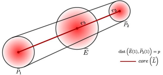
Figure 7.
Fuzzy point is fuzzily contained in .
In future research, we want to compare our results with those obtained by considering the definitions of fuzzy distance and fuzzy line segment that depend on the definitions of inverse points and same points with respect to continuous fuzzy points given in [20]. Moreover, we plan to define other secondary elements of a fuzzy triangle and study their properties or how to extend them from Euclidian geometry to analytical fuzzy geometry.
Funding
This research was funded by Universidad de Playa Ancha de Ciencias de la Educación, regular research grant 2021–2022, key project CNE 07-2223 and UPLA Foundation Projects within the framework of Execution of Diplomado Bases de la Investigación Científica.
Data Availability Statement
Not applicable.
Conflicts of Interest
The author declares no conflict of interest.
References
- Buckley, J.; Eslami, E. Fuzzy Plane Geometry. 1. Points and Lines. Fuzzy Sets Syst. 1997, 86, 179–187. [Google Scholar] [CrossRef]
- Buckley, J.; Eslami, E. Fuzzy Plane Geometry. 2. Circles and Polygons. Fuzzy Sets Syst. 1997, 87, 79–85. [Google Scholar] [CrossRef]
- Cantor, G. On a property of the class of all real algebraic numbers. Crelle’S J. Math. 1874, 77, 258–262. [Google Scholar] [CrossRef]
- Zadeh, L. Fuzzy Sets. Inf. Control 1965, 8, 338–353. [Google Scholar] [CrossRef]
- Lee, K. First Course on Fuzzy Theory and Applications; Advances in Intelligent and Soft Computing; Springer: Berlin/Heidelberg, Germany, 2005; Volume 27. [Google Scholar]
- Ahuja; Davis; Milgram; Rosenfeld. Piecewise Approximation of Pictures Using Maximal Neighborhoods. IEEE Trans. Comput. 1978, C-27, 375–379. [Google Scholar] [CrossRef]
- Clark, T.; Larson, J.; Mordeson, J.; Potter, J.; Wierman, M. Applying Fuzzy Mathematics to Formal Models in Comparative Politics; Studies in Fuzziness and Soft Computing; Springer: Berlin/Heidelberg, Germany, 2008; Volume 225. [Google Scholar]
- Egusa, Y.; Akahori, H.; Morimura, A.; Wakami, N. An Application of Fuzzy Set Theory for an Electronic Video Camera Image Stabilizer. IEEE Trans. Fuzzy Syst. 1995, 3, 351–356. [Google Scholar] [CrossRef]
- Lingala, M.; Joe Stanley, R.; Rader, R.; Hagerty, J.; Rabinovitz, H.; Oliviero, M.; Choudhry, I.; Stoecker, W. Fuzzy Logic Color Detection: Blue Areas in Melanoma Dermoscopy Images. Comput. Med. Imaging Graph. 2014, 38, 403–410. [Google Scholar] [CrossRef] [PubMed]
- Yoshimura, S.; Mochizuki, Y.; Yagawa, G. Automated Structural Design Based on Knowledge Engineering and Fuzzy Control. Eng. Comput. 1995, 12, 593–608. [Google Scholar] [CrossRef]
- Zimmermann, H. Fuzzy Control. In Fuzzy Set Theory and Its Applications; Springer: Berlin/Heidelberg, Germany, 2001; pp. 223–264. [Google Scholar]
- Bogomolny, A. On the Perimeter and Area of Fuzzy Sets. Fuzzy Sets Syst. 1987, 23, 257–269. [Google Scholar] [CrossRef]
- Guha, D.; Chakraborty, D. A New Approach to Fuzzy Distance Measure and Similarity Measure between Two Generalized Fuzzy Numbers. Appl. Soft Comput. 2010, 10, 90–99. [Google Scholar] [CrossRef]
- Gupta, K.; Ray, S. Fuzzy Plane Projective Geometry. Fuzzy Sets Syst. 1993, 54, 191–206. [Google Scholar] [CrossRef]
- Li, Q.; Guo, S. Fuzzy Geometric Object Modelling. In Proceedings of the Fuzzy Information and Engineering; Cao, B., Ed.; Springer: Berlin/Heidelberg, Germany, 2007; pp. 551–563. [Google Scholar]
- Löffler, M.; Kreveld, M. Geometry with Imprecise Lines. In Proceedings of the 24th European Workshop on Computational Geometry, Nancy, France, 18–20 March 2008; Volume 40, pp. 133–136. [Google Scholar]
- Rosenfeld, A. The Diameter of a Fuzzy Set. Fuzzy Sets Syst. 1984, 13, 241–246. [Google Scholar] [CrossRef]
- Rosenfeld, A. Fuzzy Plane Geometry: Triangles. Pattern Recognit. Lett. 1994, 15, 1261–1264. [Google Scholar] [CrossRef]
- Rosenfeld, A. Fuzzy Geometry: An Updated Overview. Inf. Sci. 1998, 110, 127–133. [Google Scholar] [CrossRef]
- Ghosh, D.; Chakraborty, D. Analytical Fuzzy Plane Geometry I. Fuzzy Sets Syst. 2012, 209, 66. [Google Scholar] [CrossRef]
- Ghosh, D.; Chakraborty, D. An Introduction to Analytical Fuzzy Plane Geometry; Springer: Berlin/Heidelberg, Germany, 2019. [Google Scholar]
- Ghosh, D.; Gupta, D.; Som, T. Analytical Fuzzy Space Geometry I. Fuzzy Sets Syst. 2021, 421, 77–110. [Google Scholar] [CrossRef]
- Ghosh, D.; Gupta, D.; Som, T. Analytical Fuzzy Space Geometry II. Fuzzy Sets Syst. 2022, 459, 144–181. [Google Scholar] [CrossRef]
- Qiu, J.; Zhang, M. Fuzzy Space Analytic Geometry. In Proceedings of the 2006 International Conference on Machine Learning and Cybernetics, Dalian, China, 13–26 August 2006; pp. 1751–1755. [Google Scholar] [CrossRef]
- Dubois, D.; Prade, H. Fuzzy Sets and Systems: Theory and Applications; Academic Press: New York, NY, USA, 1980; Volume 144. [Google Scholar]
- Conci, A.; Kubrusly, C. Distances between Sets. Sci. Appl. 2017, 26, 1–18. [Google Scholar]
- Gardner, R. Geometric Tomography; Cambridge University Press: Cambridge, UK, 1995; Volume 6. [Google Scholar]
- Schneider, R. Convex Bodies: The Brunn–Minkowski Theory; Number 151 in Encyclopedia of Mathematics and Its Applications; Cambridge University Press: Cambridge, UK, 2014. [Google Scholar]
- Alber, Y. Generalized Projections, Decompositions, and the Pythagorean-type Theorem in Banach Spaces. Appl. Math. Lett. 1998, 11, 115–121. [Google Scholar] [CrossRef]
- Amari, S. Information Geometry and Its Applications: Convex Function and Dually Flat Manifold. In Emerging Trends in Visual Computing. ETVC 2008; Lecture Notes in Computer Science; Nielsen, F., Ed.; Springer: Berlin/Heidelberg, Germany, 2009; Volume 5416, pp. 75–102. [Google Scholar] [CrossRef]
- Conant, D.; Beyer, W. Generalized Pythagorean Theorem. Am. Math. Mon. 1974, 81, 262–265. [Google Scholar] [CrossRef]
- Ungar, A. The Hyperbolic Pythagorean Theorem in the Poincaré Disc Model of Hyperbolic Geometry. Am. Math. Mon. 1999, 106, 759–763. [Google Scholar] [CrossRef]
- Chakraborty, D.; Das, S. Fuzzy Geometry: Perpendicular to Fuzzy Line Segment. Inf. Sci. 2018, 468, 213–225. [Google Scholar] [CrossRef]


Disclaimer/Publisher’s Note: The statements, opinions and data contained in all publications are solely those of the individual author(s) and contributor(s) and not of MDPI and/or the editor(s). MDPI and/or the editor(s) disclaim responsibility for any injury to people or property resulting from any ideas, methods, instructions or products referred to in the content. |
© 2023 by the author. Licensee MDPI, Basel, Switzerland. This article is an open access article distributed under the terms and conditions of the Creative Commons Attribution (CC BY) license (https://creativecommons.org/licenses/by/4.0/).