Surface Family with Bertrand Curves as Joint Asymptotic Curves in 3D Galilean Space

Abstract

The primary objective of this work is to discuss a surface family with the similarity of Bertrand curves in 3D Galilean space. Subsequently, by applying the Serret–Frenet frame, we estimate the sufficient and necessary statuses of a surface family with Bertrand curves as joint asymptotic curves. The dilation to ruled surfaces is also summarized. Meanwhile, the epitomes are illustrated to provide an explanation of the theoretical results.

1. Introduction

The geometric design of a surface is the quintessence of meaning in Computer-Aided Geometric Design. Nowadays, considerable studies are being undertaken to design a surface family with a specific curve. In Euclidean 3-space ${\mathbb{E}}^3$, Wang et al. [1] considered a surface family with a joint geodesic. The diverse marching-scale functions are examined in [2]. Li et al. defined a surface family and a developable surface family with a joint curvature line, respectively, in [3,4]. Bayram et al. [5] and Liu et al. [6] examined a surface family and a developable surface family with a joint asymptotic curve, respectively. Further, some distinctive curves have been addressed to design a surface family, e.g., the Smarandache curve is considered to be geodesic to design a surface family with various frames in [7,8]. Bayram [9] specified a surface family with an involute curve to be an asymptotic curve. Guler [10] considered an offset surface family with a joint asymptotic curve. Atalay [11,12] defined a surface family with Mannheim curves to be asymptotic curves and geodesic, respectively. R. A. Abdel-Baky and N. Alluhaib [13] examined a surface family and developable surface family with a joint geodesic curve.

Galilean geometry is the simplest model of semi-Euclidean geometry in which the isotropic cone reduces to a plane. It is demonstrated as a bridge from Euclidean geometry to special relativity. The prime divergence of Galilean geometry is its private gravity, as it allows the scientist to explore it in detail without losing a large amount of time and debater energy. Put differently, the visibility of Galilean geometry forms its growth with a simple question, and overall extension of a new geometric organization is essential for its effective rapprochement with Euclidean geometry. Also, overall development is feasible to provide the scientist the psychological assurance of the consistency of the examined structure [14]. In the $3\mathbb{D}$ (three-dimensional) Galilean space ${\mathbb{G}}_3$, reports on the appropriate steps on surfaces with an asymptotic curve are scarce. This is a significant and enchanting issue in functional applications. Artikbaev and Saitova [15] gave essential concepts of the geometry of 3D spaces in vector formulation in an affine vector space $A_n$. Dede et al. [16,17] resolved tub surfaces and the descriptions of parallel surfaces. Yuzbas et al. [18,19] considered a surface family with a curve that is joint asymptotic curve and geodesic, respectively. Jiang et al. [20] considered a surface pencil pair with a Bertrand pair as joint asymptotic curves. Almoneef and Abdel-Baky [21] designed a surface family with Bertrand curves to be geodesic curves. AL-Jedani and Abdel-Baky [22] inspected a surface family and developable surface family with a joint geodesic curve.

In this paper, we adopt an elegant manner for designing a surface family with a Bertrand pair as joint asymptotic curves. Given the allowable curves, we initially question a condition that is both sufficient and necessary for the specified curves to be asymptotic Bertrand curves. In the procedure of conclusion, the sufficient and necessary conditions when the resulting surface family is a ruled surface family are also analyzed. Meanwhile, different representative curves are selected to confirm the manner. The paramount point to note here is the manner we have utilized (compared with [20]).

2. Basic Concepts

The $3\mathbb{D}$ (three-dimensional) Galilean space ${\mathbb{G}}_3$ is a Cayley–Klein geometry contributed via the projective metric of signature $(0,0,+,+)$ [14,23,24]. The absolute figure of the Galilean space is contingent on the arranged triad {$\omega$, f, I}, where $\omega$ is the (absolute) plane in the real 3D projective space ${\mathbb{P}}^3$($\mathbb{R}$), f is the line (absolute line) in $\omega$, and I the steady elliptic involution of points of f. Homogeneous coordinates in ${\mathbb{G}}_3$ are offered in such a way that the absolute plane $\omega$ is specified by $x_0=0$, the absolute line f by $x_0=x_1=0$, and the elliptic involution by $(0:0:x_2:x_3)\to (0:0:x_3:-x_2)$. A plane is named Euclidean if it contains f; on the other hand, it is named isotropic—that is, if planes x = const. are Euclidean—as is the plane $\omega$. Other planes are isotropic. Further, an isotropic plane does not involve any isotropic orientation.

For any $\mathit{\gamma }=\left({\gamma }_1,{\gamma }_2,{\gamma }_3\right)$ and $\mathit{\beta }$ $=\left({\beta }_1,{\beta }_2,{\beta }_3\right)\in {\mathbb{G}}_3$, their scalar Galilean product is

$$<\mathit{\gamma },\mathit{\beta }>=\left\{\begin{array}{c}{\gamma }_1{\beta }_1,\mathrm{if}{\gamma }_1\ne 0\vee {\beta }_1\ne 0\hfill \\ {\gamma }_2{\beta }_2+{\gamma }_3{\beta }_3,\mathrm{if}{\gamma }_1=0\wedge {\beta }_1=0,\hfill \end{array}\right.$$

(1)

and their vector Galilean product is

$$\mathit{\gamma }\times \mathit{\beta }=\left\{\begin{array}{c}\left|\begin{array}{ccc}\mathbf{0}\hfill & \mathit{j}\hfill & \mathit{k}\hfill \\ {\gamma }_1\hfill & {\gamma }_2\hfill & {\gamma }_3\hfill \\ {\beta }_1\hfill & {\beta }_2\hfill & {\beta }_3\hfill \end{array}\right|,\mathrm{if}{\gamma }_1\ne 0\vee {\beta }_1\ne 0,\\ \left|\begin{array}{ccc}\mathit{i}\hfill & \mathit{j}\hfill & \mathit{k}\hfill \\ 0\hfill & {\gamma }_2\hfill & {\gamma }_3\hfill \\ 0\hfill & {\beta }_2\hfill & {\beta }_3\hfill \end{array}\right|,\mathrm{if}{\gamma }_1=0\wedge {\beta }_1=0.\end{array}\right.$$

(2)

where $\mathit{i}=(1,0,0)$, $\mathit{j}=(0,1,0)$, and $\mathit{k}=(0,0,1)$ are the standard basis vectors in ${\mathbb{G}}_3$.

A curve $\mathit{\beta }$$\left(u\right)=\left({\beta }_1\left(u\right),{\beta }_2\left(u\right),{\beta }_3\left(u\right)\right);u\in I\subseteq \mathbb{R}$. A curve is said to be an allowable curve if it has no inflection points, $\stackrel{.}{\mathit{\beta }}\times \stackrel{..}{\mathit{\beta }}\ne \mathbf{0}$, and no isotropic tangents, $\stackrel{.}{{\beta }_1}\ne 0$. An allowable curve is similar to a smooth curve in Euclidean space. For an allowable curve $\mathit{\beta }$: $I\subseteq \mathbb{R}\to {\mathbb{G}}_3$ represented by the Galilean invariant arc-length s, we have

$$\mathit{\beta }\left(s\right)=\left(s,{\beta }_2\left(s\right),{\beta }_3\left(s\right)\right).$$

(3)

The curvature $\kappa \left(s\right)$ and torsion $\tau \left(s\right)$ of the curve $\mathit{\beta }$$\left(s\right)$ are

$$\begin{array}{ccc}\hfill \kappa \left(s\right)& =& ∥{\mathit{\beta }}^{{}^{″}}\left(s\right)∥=\sqrt{{\left({\beta }_2^{{}^{″}}\left(s\right)\right)}^2+{\left({\beta }_3^{{}^{″}}\left(s\right)\right)}^2},\hfill \\ \hfill \tau \left(s\right)& =& \frac{1}{{\kappa }^2\left(s\right)}det\left({\mathit{\beta }}^{\prime },{\mathit{\beta }}^{″},{\mathit{\beta }}^{‴}\right).\hfill \end{array}$$

(4)

Note that an allowable curve has $\kappa \left(s\right)\ne 0$. The affiliated Serret–Frenet vectors are

$$\begin{array}{ccc}\hfill \mathit{\upsilon }\left(s\right)& =& {\mathit{\beta }}^{{}^{\prime }}\left(s\right)=\left(1,{\beta }_2^{{}^{\prime }}\left(s\right),{\beta }_3^{{}^{\prime }}\left(s\right)\right),\hfill \\ \hfill \mathit{\varsigma }\left(s\right)& =& \frac{1}{\kappa \left(s\right)}{\mathit{\beta }}^{{}^{\prime }}\left(s\right)=\frac{1}{\kappa \left(s\right)}\left(0,{\beta }_2^{{}^{″}}\left(s\right),{\beta }_3^{{}^{″}}\left(s\right)\right),\hfill \\ \hfill \mathit{\eta }\left(s\right)& =& \frac{1}{\tau \left(s\right)}\left(0,{\left(\frac{1}{\kappa \left(s\right)}{\beta }_2^{{}^{″}}\left(s\right)\right)}^{{}^{\prime }},{\left(\frac{1}{\kappa \left(s\right)}{\beta }_3^{{}^{″}}\left(s\right)\right)}^{{}^{\prime }}\right),\hfill \end{array}$$

(5)

where $\mathit{\upsilon }\left(s\right)$, $\mathit{\varsigma }$$\left(s\right)$, and $\mathit{\eta }$$\left(s\right)$, respectively, are the tangent, principal normal, and binormal vectors. For every point of $\mathit{\beta }$$\left(s\right)$, the Serret–Frenet formulae read

$$\left(\begin{array}{c}{\mathit{\upsilon }}^{{}^{\prime }}\hfill \\ {\mathit{\varsigma }}^{{}^{\prime }}\hfill \\ {\mathit{\eta }}^{{}^{\prime }}\hfill \end{array}\right)=\left(\begin{array}{ccc}0\hfill & \kappa \left(s\right)\hfill & 0\hfill \\ 0\hfill & 0\hfill & \tau \left(s\right)\hfill \\ 0\hfill & -\tau \left(s\right)\hfill & 0\hfill \end{array}\right)\left(\begin{array}{c}\mathit{\upsilon }\hfill \\ \mathit{\varsigma }\hfill \\ \mathit{\eta }\hfill \end{array}\right).$$

(6)

The planes that match to the subspaces $Sp\{\mathit{\upsilon },$ $\mathit{\varsigma }$}, $Sp\{$$\mathit{\varsigma }$, $\mathit{\eta }$}, and $Sp\{$$\mathit{\eta }$, $\mathit{\upsilon }\}$, respectively, are named the osculating plane, normal plane, and rectifying plane.

Definition 1

([20,21,22]). Let β$\left(s\right)$ and $\widehat{\mathit{\beta }}\left(s\right)$ be two allowable curves in ${\mathbb{G}}^3$. Both curves in the pair {$\widehat{\mathit{\beta }}\left(s\right)$, β$\left(s\right)$} are named Bertrand curves (mates) if the principal normals, ς$\left(s\right)$ of β$\left(s\right)$ and $\widehat{\mathit{\varsigma }}\left(s\right)$ of $\widehat{\mathit{\beta }}\left(s\right)$, are linearly dependent—that is,

$$\widehat{\mathit{\beta }}\left(s\right)=\mathit{\beta }\left(s\right)+f\mathit{\varsigma }\left(s\right).$$

(7)

where f is a constant.

We signalize a surface M in ${\mathbb{G}}_3$ by

$$M:\mathit{y}(s,\chi )=\left(y_1\left(s,\chi \right),y_2\left(s,\chi \right),y_3\left(s,\chi \right)\right),(s,\chi )\in \mathbb{D}\subseteq {\mathbb{R}}^2.$$

(8)

If ${\mathit{y}}_j(s,\chi )=\frac{\partial y}{\partial j}$, the isotropic surface normal is

$$\mathit{\xi }(s,\chi )={\mathit{y}}_s\wedge {\mathit{y}}_{\chi },$$

(9)

which is perpendicular to each of the vectors ${\mathit{y}}_s$ and ${\mathit{y}}_{\chi }$.

Definition 2

([20,21,22]). A curve on a surface is asymptotic if and only if the surface normal is parallel to the binormal vector of the curve.

An isoparametric curve is a curve $\mathit{\beta }$$\left(s\right)$ on a surface $\mathit{y}(s,\chi )$ that has a stationary s- or $\chi$-parameter value. In other words, there exists a parameter ${\chi }_0$ such that $\mathit{\beta }$$\left(s\right)=\mathit{y}(s,{\chi }_0)$ or $\mathit{\beta }$$\left(\chi \right)=\mathit{y}(s_0,\chi )$. Given a parametric curve $\beta \left(s\right)$, we call it an isoasymptote of the surface $\mathit{y}(s,\chi )$ if it is both an asymptotic and parameter curve on $\mathit{y}(s,\chi )$.

3. Main Results

This section displays an approach to organizing a surface family with two Bertrand curves as joint asymptotic curves. Therefore, we take into computation the Bertrand curves such that the tangent planes of the surface family are concomitant with the osculating planes of the two curves.

Let {$\widehat{\mathit{\beta }}\left(s\right)$, $\mathit{\beta }$$\left(s\right)$} be allowable Bertrand curves, and $\{\widehat{\mathit{\beta }};$ $\widehat{\mathit{\upsilon }},\widehat{\mathit{\varsigma }},\widehat{\mathit{\eta }}\}$ are declared in Equations (3)–(6). By making the surface tangent plane coincide with the curve osculating plane, the surface M with $\mathit{\beta }$$\left(s\right)$ is expounded by

$$M:\mathit{y}(s,\chi )=\mathit{\beta }\left(s\right)+a(s,\chi )\mathit{\upsilon }\left(s\right)+b(s,\chi )\mathit{\varsigma }(s);0\le \chi \le \chi .$$

(10)

Similarly, the surface $\widehat{M}$ with $\widehat{\mathit{\beta }}\left(s\right)$ is expounded by

$$\widehat{M}:\widehat{\mathit{y}}(s,\chi )=\widehat{\mathit{\beta }}\left(s\right)+a(s,\chi )\widehat{\mathit{\upsilon }}\left(s\right)+b(s,\chi )\widehat{\mathit{\varsigma }}\left(s\right);0\le \chi \le \chi .$$

(11)

Here, $a(s,\chi )$ and $b(s,\chi )$ are named as directed marching-scale functions with $b(s,\chi )\ne 0$. The paramount point to note here is the manner we have utilized (compared with [20]).

In order to manifest that $\mathit{\beta }$$\left(s\right)$ is an asymptotic curve on M, via Equation (10), we investigate what the marching-scale functions should satisfy. Thus, we have

$$\left.\begin{array}{c}{\mathit{y}}_s(s,\chi )=(1+a_s)\mathit{\upsilon }+(a\kappa +{\eta }_s)\mathit{\varsigma }+\tau b\mathit{\eta },\hfill \\ {\mathit{y}}_{\chi }(s,\chi )=a_{\chi }\mathit{\upsilon }+b_{\chi }\mathit{\varsigma }.\hfill \end{array}\right\}$$

(12)

The normal vector of M can be expounded by

$$\mathit{\xi }(s,\chi ):={\mathit{y}}_s\times {\mathit{y}}_{\chi }=\tau b{a}_{\chi }\mathit{\upsilon }+\left[(1+a_s)b_{\chi }-(\kappa a+{\eta }_s)a_{\chi }\right]\mathit{\eta }.$$

(13)

Also, since the curve $\mathit{\beta }$$\left(s\right)$ is isoparametric on the surface, there exists a parameter $\chi ={\chi }_0\in [0,\chi ]$ such that $\mathit{y}(s,{\chi }_0)=$ $\mathit{\beta }$$\left(s\right)$—that is,

$$a(s,{\chi }_0)=b(s,{\chi }_0)=0,a_s(s,{\chi }_0)=b_s(s,{\chi }_0)=0.$$

(14)

Thus, when $\chi ={\chi }_0$—i.e., over the curve $\mathit{\beta }$$\left(s\right)$—the surface normal is

$$\mathit{\xi }(s,{\chi }_0)=b_{\chi }(s,{\chi }_0)\mathit{\eta }\left(s\right).$$

(15)

Coincidence of the surface normal $\mathit{\xi }$ with the binormal $\mathit{\eta }$$\left(s\right)$ identifies the curve as an asymptotic curve. We set {$\widehat{M}$, M} to symbolize the surface family. Hence, combining Equations (13) and (14), the next theorem is given:

Theorem 1.

{M, $\widehat{M}$} interpolate { β$\left(s\right)$, $\widehat{\mathit{\beta }}\left(s\right)$} as joint asymptotic Bertrand curves if and only if

$$\left.\begin{array}{c}a(s,{\chi }_0)=b(s,{\chi }_0)=0,0\le {\chi }_0\le \chi ,0\le s\le L,\hfill \\ (1+a_s(s,{\chi }_0))b_{\chi }(s,{\chi }_0)-b_s(s,{\chi }_0)a_{\chi }(s,{\chi }_0)\ne 0.\hfill \end{array}\right\}$$

(16)

Noteworthily, any surface M ($\widehat{M}$) described by Equations (10) and (11) and fulfilling Equation (16) is a constituent of the surface family with asymptotic curve $\mathit{\beta }$$\left(s\right)$ ($\widehat{\mathit{\beta }}\left(s\right))$. Equation (16) is more convenient and elegant for implementations than that reported in [1]. In order to resolve the situations in Theorem 1 simply, the functions $a(s,\chi ),$ and $b(s,\chi )$ can be expounded by

$$\begin{array}{c}a(s,\chi )=l\left(s\right)A\left(\chi \right),\\ b(s,\chi )=m\left(s\right)B\left(\chi \right).\end{array}$$

(17)

Here $l\left(s\right)$, $m\left(s\right),A\left(\chi \right)$, and $B\left(\chi \right)$ are $C^1$ functions that are not identically zero. Hence, from Theorem 1, we can give the following corollary.

Corollary 1.

{M, $\widehat{M}$} interpolate {β$\left(s\right)$, $\widehat{\mathit{\beta }}\left(s\right)$} as joint asymptotic Bertrand curves if and only if

$$\left.\begin{array}{c}A\left({\chi }_0\right)=B\left({\chi }_0\right)=0,l\left(s\right)=const.,m\left(s\right)=const.\ne 0,\hfill \\ \frac{db\left({\chi }_0\right)}{d\chi }=const.\ne 0,0\le {\chi }_0\le \chi ,0\le s\le L.\hfill \end{array}\right\}$$

(18)

Now, we establish other sorts of marching-scale functions:

(1) If

$$\left\{\begin{array}{c}a(s,\chi )=\underset{k=1}{\stackrel{p}{\Sigma }}{a}_{1k}l{\left(s\right)}^{k}A{\left(\chi \right)}^k,\\ b(s,\chi )=\underset{k=1}{\stackrel{p}{\Sigma }}{b}_{1k}m{\left(s\right)}^{k}B{\left(\chi \right)}^k,\end{array}\right.$$

(19)

then

$$\left\{\begin{array}{c}A\left({\chi }_0\right)=B\left({\chi }_0\right)=0,\\ b_{11}\ne 0,m\left(s\right)\ne 0,\mathrm{and}\frac{dV\left({\chi }_0\right)}{d\chi }\ne 0,\end{array}\right.$$

(20)

where $l\left(s\right),$ $m\left(s\right),$ $A\left(\chi \right),$ and $\eta \left(\chi \right)$ are $C^1$ functions; $a_{ij}$, $b_{ij}\in \mathbb{R}$$(i=1,2;j=1,2,...,p)$; and $l\left(s\right)$ and $m\left(s\right)$ are not identically zero.

(2) If

$$\left\{\begin{array}{c}a(s,\chi )=f\left(\underset{k=1}{\stackrel{p}{\Sigma }}{a}_{1k}{l}^k\left(s\right)A^k\left(\chi \right)\right),\\ b(s,\chi )=g\left(\underset{k=1}{\stackrel{p}{\Sigma }}{b}_{1k}{m}^k\left(s\right)B^k\left(\chi \right)\right),\end{array}\right.$$

(21)

then

$$\left\{\begin{array}{c}A\left({\chi }_0\right)=B\left({\chi }_0\right)=a\left({\chi }_0\right)=f\left(0\right)=g\left(0\right)=0,\\ b_{11}\ne 0,\frac{db\left({\chi }_0\right)}{d\chi }=const\ne 0,m\left(s\right)\ne 0,g^{{}^{\prime }}\left(0\right)\ne 0,\end{array}\right.$$

(22)

where $l\left(s\right),$ $m\left(s\right),$ $A\left(\chi \right),$ $B\left(\chi \right)$, f, and g are $C^1$ functions. Since there are no constraints joined to the specified curve in Equations (18), (20), or (22), the set {$\widehat{M}$, M} interpolating {$\mathit{\beta }\left(s\right)$, $\widehat{\mathit{\beta }}\left(s\right)$} as common asymptotic Bertrand curves can permanently be offered by choosing convenient marching-scale functions.

Example 1.

Let β$\left(s\right)$ be an allowable helix pointed by

$$\mathit{\beta }\left(s\right)=(s,sins,coss),0\le s\le 2\pi .$$

Then,

$$\begin{array}{ccc}\hfill {\mathit{\beta }}^{{}^{\prime }}\left(s\right)& =& (1,coss,-sins),\hfill \\ \hfill {\mathit{\beta }}^{{}^{″}}\left(s\right)& =& (0,-sins,-coss),\hfill \\ \hfill {\mathit{\beta }}^{{}^{{}^{‴}}}\left(s\right)& =& (0,-coss,sins).\hfill \end{array}$$

Use Equations (3)–(5) to gain $\kappa \left(s\right)=1,\tau \left(s\right)=1$, and

$$\begin{array}{ccc}\hfill \mathit{\upsilon }(s)& =& (1,coss,-sins),\hfill \\ \hfill \mathit{\varsigma }(s)& =& (0,-sins,-coss),\hfill \\ \hfill \mathit{\eta }(s)& =& (0,coss,-sins).\hfill \end{array}$$

Let $f=2$ in Equation (7); we obtain $\widehat{\mathit{\beta }}\left(s\right)=(s,-sins,-coss)$ and

$$\begin{array}{ccc}\hfill \widehat{\mathit{\upsilon }}\left(s\right)& =& (1,-coss,sins),\hfill \\ \hfill \widehat{\mathit{\varsigma }}\left(s\right)& =& (0,sins,coss),\hfill \\ \hfill \widehat{\mathit{\eta }}\left(s\right)& =& (0,-coss,sins).\hfill \end{array}$$

According to Corollary 1, we have the following:

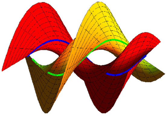
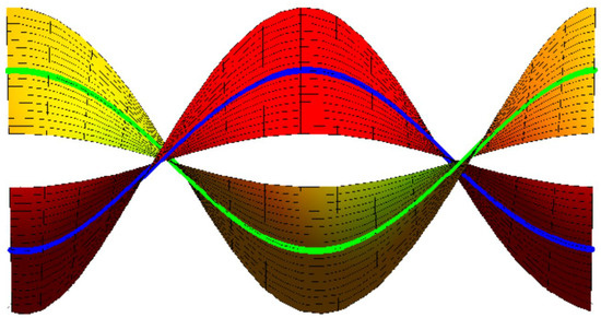
(A). If $a(s,\chi )=\chi$, $b(s,\chi )=2\chi$, and ${\chi }_0=0$, Equation (18) is fulfilled. The set {M, $\widehat{M}$} interpolating {β$\left(s\right)$, $\widehat{\mathit{\beta }}\left(s\right)$} as joint asymptotic Bertrand curves is (Figure 1)

$$\left\{\begin{array}{c}M:\mathit{y}(s,\chi )=(s+\chi ,(1-2\chi )sins+\chi coss,(1-2\chi )coss-\chi sins),\\ \widehat{M}:\widehat{\mathit{y}}(s,\chi )=(s+\chi ,-(1-2\chi )sins-\chi coss,-(1-2\chi )coss+\chi sins),\end{array}\right.$$

where the blue curve depicts β$\left(s\right)$, the green curve is $\widehat{\mathit{\beta }}\left(s\right)$, $-1\le$$\chi \le 1$, and $0\le$ $s\le 2\pi$.

Figure 1. M, yellow; $\widehat{M}$, red.

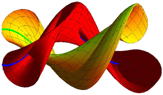
(B). If $a(s,\chi )=1-cot\chi$, $b(s,\chi )=sin\chi$, and ${\chi }_0=0$, Equation (18) is fulfilled. The set {M, $\widehat{M}$} interpolating {β$\left(s\right)$, $\widehat{\mathit{\beta }}\left(s\right)$} as joint asymptotic Bertrand curves is (Figure 2)

$$M:\mathit{y}(s,\chi )=\left(\begin{array}{c}s+1-cot\chi \\ sins+\left(sin\chi +1-cot\chi \right)coss\\ coss-\left(sin\chi +1-cot\left(\chi \right)\right)sins\end{array}\right),$$

and

$$\widehat{M}:\widehat{\mathit{y}}(s,\chi )=\left(\begin{array}{c}s+1-cot\chi \\ -sins-\left(sin\chi +1-cot\chi \right)coss\\ coss-\left(-sin\chi +1-cot\left(\chi \right)\right)sins\end{array}\right),$$

where the blue curve depicts β$\left(s\right)$, the green curve is $\widehat{\mathit{\beta }}\left(s\right)$, $0\le$ s, and $\chi \le 2\pi$.

Figure 2. M, yellow; $\widehat{M}$, red.

It should be noted that we could extend this sequence of surfaces by selecting yet another characteristic curve combination or number of curves to interpolate.

Ruled Surface Family with Joint Bertrand Asymptotic Curves

Suppose ${\mathit{y}}_i(s,\chi )$ is a ruled surface with the directrix $\mathit{\beta }$${}_i\left(s\right)$ and $\mathit{\beta }$${}_i\left(s\right)$ is an isoparametric curve of ${\mathit{y}}_i(s,\chi )$; then, there exists ${\chi }_0$ such that ${\mathit{y}}_i(s,{\chi }_0)=$ $\mathit{\beta }$${}_i\left(s\right)$. This means that the surface can be stated as

$$M_i:{\mathit{y}}_i(s,\chi )-{\mathit{y}}_i(s,{\chi }_0)=(\chi -{\chi }_0){\mathit{e}}_i\left(s\right),0\le s\le L,\mathrm{with}\chi ,{\chi }_0\in [0,\chi ],$$

where ${\mathit{y}}_i(s,{\chi }_0)=$ $\mathit{\beta }$${}_i\left(s\right)$ ($i=1,2,3)$ and ${\mathit{e}}_i\left(s\right)$ defines the direction of the rulings. According to Equation (10), we have

$$(\chi -{\chi }_0){\mathit{e}}_i\left(s\right)=a(s,\chi ){\mathit{\upsilon }}_i\left(s\right)+b(s,\chi ){\mathit{\varsigma }}_i\left(s\right),0\le s\le L,\mathrm{with}\chi ,{\chi }_0\in [0,\chi ],$$

(23)

which is a system of two equations with two unknown functions $a(s,\chi )$ and $b(s,\chi )$. To solve $a(s,\chi )$ and $b(s,\chi )$, we have

$$\begin{array}{c}a(s,\chi )=(\chi -{\chi }_0)<{\mathit{e}}_i\left(s\right),{\mathit{\upsilon }}_i\left(s\right)>,\\ b(s,\chi )=(\chi -{\chi }_0)<{\mathit{e}}_i\left(s\right),{\mathit{\varsigma }}_i\left(s\right)>.\end{array}$$

(24)

The above equations are just the necessary and sufficient conditions for which ${\mathit{y}}_i(s,\chi )$ is a ruled surface with a directrix $\mathit{\beta }$${}_i\left(s\right)$; $i=1,2,3$.

In Galilean 3-space ${\mathbb{G}}_3$, it is demonstrated that there exist only three types of ruled surfaces, specified as follows [24]:

Type I.

Non-conoidal or conoidal ruled surfaces with a striction curve that does not lie in a Euclidean plane.

Type II.

Ruled surfaces with a striction curve in a Euclidean plane.

Type III.

Conoidal ruled surfaces with an absolute line as the oriented line in infinity.

We now check if the curve $\mathit{\beta }$${}_i\left(s\right)$ is also asymptotic on these three types:

Type I.

$\mathit{\beta }$${}_1\left(s\right)=(s,y\left(s\right),z\left(s\right))$ does not lie in a Euclidean plane and ${\mathit{e}}_1\left(s\right)=(1,e_2\left(s\right),e_3\left(s\right))$ is non-isotropic. The associated Serret–Frenet frame is identified by

$$\begin{array}{ccc}\hfill {\mathit{\upsilon }}_1\left(s\right)& =& \left(1,y^{{}^{\prime }}\left(s\right),z^{{}^{\prime }}\left(s\right)\right),\hfill \\ \hfill {\mathit{\varsigma }}_1\left(s\right)& =& \frac{1}{\kappa \left(s\right)}\left(0,y^{{}^{″}}\left(s\right),z^{{}^{″}}\left(s\right)\right),\hfill \\ \hfill {\mathit{\eta }}_1\left(s\right)& =& \frac{1}{\kappa \left(s\right)}\left(0,-z^{{}^{″}}\left(s\right),y^{{}^{″}}\left(s\right)\right),\hfill \end{array}$$

(25)

where $\kappa \left(s\right)=\sqrt{{\left(y^{{}^{″}}\left(s\right)\right)}^2+{\left(z^{{}^{″}}\left(s\right)\right)}^2}$. From Equations (18) and (19), we have

$$a(s,\chi )=(\chi -{\chi }_0),b(s,\chi )=0,$$

(26)

which does not fulfill Theorem 1.

Type II.

$\mathit{\beta }$${}_2\left(s\right)=(0,y\left(s\right),z\left(s\right))$ lies in a Euclidean plane and ${\mathit{e}}_2\left(s\right)=(1,e_2\left(s\right),e_3\left(s\right))$ is non-isotropic. Similarly, we have

$$\begin{array}{ccc}\hfill {\mathit{\upsilon }}_2\left(s\right)& =& \left(0,y^{{}^{\prime }}\left(s\right),z^{{}^{\prime }}\left(s\right)\right),\hfill \\ \hfill {\mathit{\varsigma }}_2\left(s\right)& =& \frac{1}{\kappa \left(s\right)}\left(0,y^{{}^{″}}\left(s\right),z^{{}^{″}}\left(s\right)\right),\hfill \\ \hfill {\mathit{\eta }}_2\left(s\right)& =& \frac{1}{\kappa \left(s\right)}\left(0,0,0\right),\hfill \end{array}$$

(27)

where $\kappa \left(s\right)=\sqrt{{\left(y^{{}^{″}}\left(s\right)\right)}^2+{\left(z^{{}^{″}}\left(s\right)\right)}^2}$. From Equations (18) and (21), we have

$$a(s,\chi )=b(s,\chi )=0,$$

(28)

which does not fulfill Theorem 1.

Corollary 2.

There is no ruled surface family of type I and II with joint Bertrand asymptotic curves in ${\mathbb{G}}_3$.

Type III.

β${}_3\left(s\right)=(s,y\left(s\right),0)$ does not lie in a Euclidean plane and ${\mathit{e}}_3\left(s\right)=(0,e_2\left(s\right),e_3\left(s\right))$ is non-isotropic. Then,

$$\begin{array}{ccc}\hfill {\mathit{\upsilon }}_3\left(s\right)& =& \left(1,y^{\prime }\left(s\right),0\right),\hfill \\ \hfill {\mathit{\varsigma }}_3\left(s\right)& =& \frac{1}{\kappa \left(s\right)}\left(0,y^{″}\left(s\right)0\right),\hfill \\ \hfill {\mathit{\eta }}_3\left(s\right)& =& \frac{1}{\kappa \left(s\right)}\left(0,0,y^{″}\left(s\right)\right),\hfill \end{array}$$

(29)

where $\kappa \left(s\right)=\left|y^{″}\left(s\right)\right|$. From Equations (18) and (24), we have

$$\left.\begin{array}{c}a(s,\chi )=0,b(s,\chi )=ϵ(\chi -{\chi }_0)e_2\left(s\right),\hfill \\ \\ e_2\left(s\right)\ne 0,{\chi }_0\ne 0,\hfill \end{array}\right\}$$

(30)

where

$$ϵ=\left\{\begin{array}{c}1,\mathrm{if}{y}^{{}^{″}}\left(s\right)>0,\\ -1,\mathrm{if}{y}^{{}^{″}}\left(s\right)<0.\end{array}\right.$$

(31)

Equation (30) fulfills Theorem 1. Similarity, the ruled surfaces $\widehat{M}$ of type III also have the curve $\mathit{\beta }$${}_3\left(s\right)$ as a joint asymptotic curve.

Hence, we have the following corollary:

Corollary 3.

The ruled surface family of type III has joint Bertrand asymptotic curves.

Now, we seek the engagements of the ruled surface family of type III. Let $\mathit{\beta }$$\left(s\right)=(s,y(s),0)$, $0\le s\le L$ be a curve with $\mathit{\beta }$${}^{{}^{″}}\left(s\right)\ne 0$ from Equations (7), (29), and (30); the Bertrand mate of $\mathit{\beta }$$\left(s\right)$ is $\widehat{\mathit{\beta }}\left(s\right)=(s,y\left(s\right)+ϵf,0)$. From Equations (10), (11), and (31), the ruled surface family of type III with joint Bertrand asymptotic curves is

$$\left\{\begin{array}{c}M:\mathit{y}(s,\chi )=(s,y\left(s\right),0)+(\chi -{\chi }_0)e_2\left(s\right)(0,1,0).\\ \widehat{M}:\widehat{\mathit{y}}(s,\chi )=(s,y\left(s\right)+f,0)+ϵ(\chi -{\chi }_0)e_2\left(s\right)(0,1,0)\end{array}\right.$$

(32)

where f is a constant, $ϵ$ fulfills Equation (31), $e_2\ne 0$, and ${\chi }_0\ne 0$.

Example 2.

In view of Example 1, we have the following:

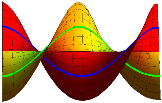
(a). If $a(s,\chi )=0$, $b(s,\chi )=sin\chi$. The ruled {M, $\widehat{M}$} interpolating {β$\left(s\right)$, $\widehat{\mathit{\beta }}\left(s\right)$} as joint asymptotic Bertrand curves is (Figure 3)

$$\left\{\begin{array}{c}M:\mathit{y}(s,\chi )=(s,sins,coss)+(0,-sins,-coss)sin\chi ,\\ \widehat{M}:\widehat{\mathit{y}}(s,\chi )=(s,-sins,-coss)+(0,sins,coss)sin\chi ,\end{array}\right.$$

where the blue curve depicts β$\left(s\right)$, the green curve is $\widehat{\mathit{\beta }}\left(s\right)$, $0\le s$, and $\chi \le 2\pi$.

Figure 3. M, yellow; $\widehat{M}$, red.

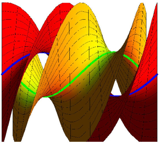
(b). If $a(s,\chi )=0$, $b(s,\chi )=\chi$. The ruled {M, $\widehat{M}$} interpolating {β$\left(s\right)$, $\widehat{\mathit{\beta }}\left(s\right)$} as joint asymptotic Bertrand curves is (Figure 4)

$$\left\{\begin{array}{c}M:\mathit{y}(s,\chi )=(s,sins,coss)+\chi (0,-sins,-coss),\\ \widehat{M}:\widehat{\mathit{y}}(s,\chi )=(s,-sins,-coss)+\chi (0,sins,coss),\end{array}\right.$$

where the blue curve depicts β$\left(s\right)$, the green curve is $\widehat{\mathit{\beta }}\left(s\right)$, $-3\le \chi \le 3$, and $0\le$$s,\chi \le 2\pi$.

Figure 4. M, yellow; $\widehat{M}$, red.

(c). If $a(s,\chi )=0$, $b(s,\chi )=-\chi$. The ruled {M, $\widehat{M}$} interpolating {β$\left(s\right)$, $\widehat{\mathit{\beta }}\left(s\right)$} as joint asymptotic Bertrand curves is (Figure 5)

$$\left\{\begin{array}{c}M:\mathit{y}(s,\chi )=(s,sins,coss)-\chi (0,-sins,-coss),\\ \widehat{M}:\widehat{\mathsf{y}}(s,\chi )=(s,-sins,-coss)-\chi (0,sins,coss),\end{array}\right.$$

where the blue curve depicts β$\left(s\right)$, the green curve is $\widehat{\mathit{\beta }}\left(s\right)$, $-0.7\le$$\chi \le 0.7$, and $0\le$ $s\le 2\pi$.

Figure 5. M, yellow; $\widehat{M}$, red.

4. Conclusions

In this work, we established the surface family and ruled surface family interpolating Bertrand curves as joint asymptotic curves in Galilean space ${\mathbb{G}}_3$. For any allowable curve, there only exists a ruled surface family of type III interpolating the curve as joint asymptotic curves. Meantime, some curves are selected to organize the surface family and ruled surface family that interpolate the Bertrand pair {$\widehat{\mathit{\beta }}\left(s\right)$, $\mathit{\beta }$$\left(s\right)$} as joint asymptotic curves. We hope that our results will be helpful to physicists and those researching general relativity. There are a lot of opportunities for further study where these results will be beneficial to anyone working in the field of computer-aided manufacturing. A parallel of the issue addressed in this paper may be plausible for the pseudo-Galilean geometry.

References

- Wang, G.J.; Tang, K.; Tai, C.L. Parametric representation of a surface pencil with a common spatial geodesic. Comput. Aided Des. 2004, 36, 447–459. [Google Scholar] [CrossRef]
- Kasap, E.; Akyldz, F.T.; Orbay, K. A generalization of surfaces family with common spatial geodesic. Appl. Math. Comput. 2008, 201, 781–789. [Google Scholar] [CrossRef]
- Li, C.Y.; Wang, R.H.; Zhu, C.G. Parametric representation of a surface pencil with a common line of curvature. Comput. Aided Des. 2011, 43, 1110–1117. [Google Scholar] [CrossRef]
- Li, C.Y.; Wang, R.H.; Zhu, C.G. An approach for designing a developable surface through a given line of curvature. Comput. Aided Des. 2013, 45, 621–627. [Google Scholar] [CrossRef]
- Bayram, E.; Guler, F.; Kasap, E. Parametric representation of a surface pencil with a common asymptotic curve. Comput. Aided Des. 2012, 44, 637–643. [Google Scholar] [CrossRef]
- Liu, Y.; Wang, G.J. Designing developable surface pencil through given curve as its common asymptotic curve. J. Zhejiang Univ. 2013, 47, 1246–1252. [Google Scholar]
- Atalay, G.S.; Kasap, E. Surfaces family with common Smarandache geodesic curve. J. Sci. Arts. 2017, 4, 651–664. [Google Scholar]
- Atalay, G.S.; Kasap, E. Surfaces family with common Smarandache geodesic curve according to Bishop frame in Euclidean space. Math. Sci. Appl. 2016, 4, 164–174. [Google Scholar] [CrossRef]
- Bayram, E. Surface family with a common involute asymptotic curve. Int. J. Geom. Methods Mod. Phys. 2016, 13, 447–459. [Google Scholar] [CrossRef]
- Guler, F.; Bayram, E.; Kasap, E. Offset surface pencil with a common asymptotic curve. Int. J. Geom. Methods Modern Phys. 2018, 15, 1850195. [Google Scholar] [CrossRef]
- Atalay, G.S. Surfaces family with a common Mannheim asymptotic curve. J. Appl. Math. Comput. 2018, 2, 143–154. [Google Scholar]
- Atalay, G.S. Surfaces family with a common Mannheim geodesic curve. J. Appl. Math. Comput. 2018, 2, 155–165. [Google Scholar]
- Abdel-Baky, R.A.; Alluhaib, N. Surfaces family with a common geodesic curve in Euclidean 3-Space . Int. J. Math. Anal. 2019, 13, 433–447. [Google Scholar] [CrossRef]
- Yaglom, I.M. A Simple Non-Euclidean Geometry and Its Physical Basis; Springer: New York, NY, USA, 1979. [Google Scholar]
- Artikbaev, A.; Saitova, S.S. Interpretation of Geometry on Manifolds as a Geometry in a Space with Projective Metric. J. Math. Sci. 2022, 265, 1–10. [Google Scholar] [CrossRef]
- Dede, M. Tubular surfaces in Galilean space. Math. Commun. 2013, 18, 209–217. [Google Scholar]
- Dede, M.; Ekici, C.; Coken, A.C. On the parallel surfaces in Galilean space. Hacet. J. Math. Stat. 2013, 42, 605–615. [Google Scholar] [CrossRef]
- Yuzbası, Z.K. On a family of surfaces with joint asymptotic curve in the Galilean space . J. Nonlinear Sci. Appl. 2016, 9, 518–523. [Google Scholar] [CrossRef][Green Version]
- Yuzbası, Z.K.; Bektas, M. On the construction of a surface family with joint geodesic in Galilean space . Open Phys. 2016, 14, 360–363. [Google Scholar] [CrossRef]
- Jiang, X.; Jiang, P.; Meng, J.; Wang, K. Surface pencil pair interpolating Bertrand pair as joint asymptotic curves in Galilean space. Int. J. Geom. Methods Modern Phys. 2021, 18, 2150114. [Google Scholar] [CrossRef]
- Almoneef, A.A.; Abdel-Baky, R.A. Surface family pair with Bertrand pair as joint geodesic curves in Galilean 3-space . Mathematics 2023, 11, 2391. [Google Scholar] [CrossRef]
- Al-Jedani, A.; Abdel-Baky, R.A. A surface family with a mutual geodesic curve in Galilean 3-space . Mathematics 2023, 11, 2971. [Google Scholar] [CrossRef]
- Roschel, O. Die Geometrie des Galileischen Raumes; Habilitationsschrift: Leoben, Austria, 1984. [Google Scholar]
- Divjak, B. Geometrija Pseudogalilejevih Prostora. Ph.D. Thesis, University of Zagreb, Zagreb, Croatia, 1997. [Google Scholar]
Disclaimer/Publisher’s Note: The statements, opinions and data contained in all publications are solely those of the individual author(s) and contributor(s) and not of MDPI and/or the editor(s). MDPI and/or the editor(s) disclaim responsibility for any injury to people or property resulting from any ideas, methods, instructions or products referred to in the content. |
© 2023 by the authors. Licensee MDPI, Basel, Switzerland. This article is an open access article distributed under the terms and conditions of the Creative Commons Attribution (CC BY) license (https://creativecommons.org/licenses/by/4.0/).