
Statistical Analysis of Inverse Weibull Constant-Stress Partially Accelerated Life Tests with Adaptive Progressively Type I Censored Data


Abstract
:1. Introduction
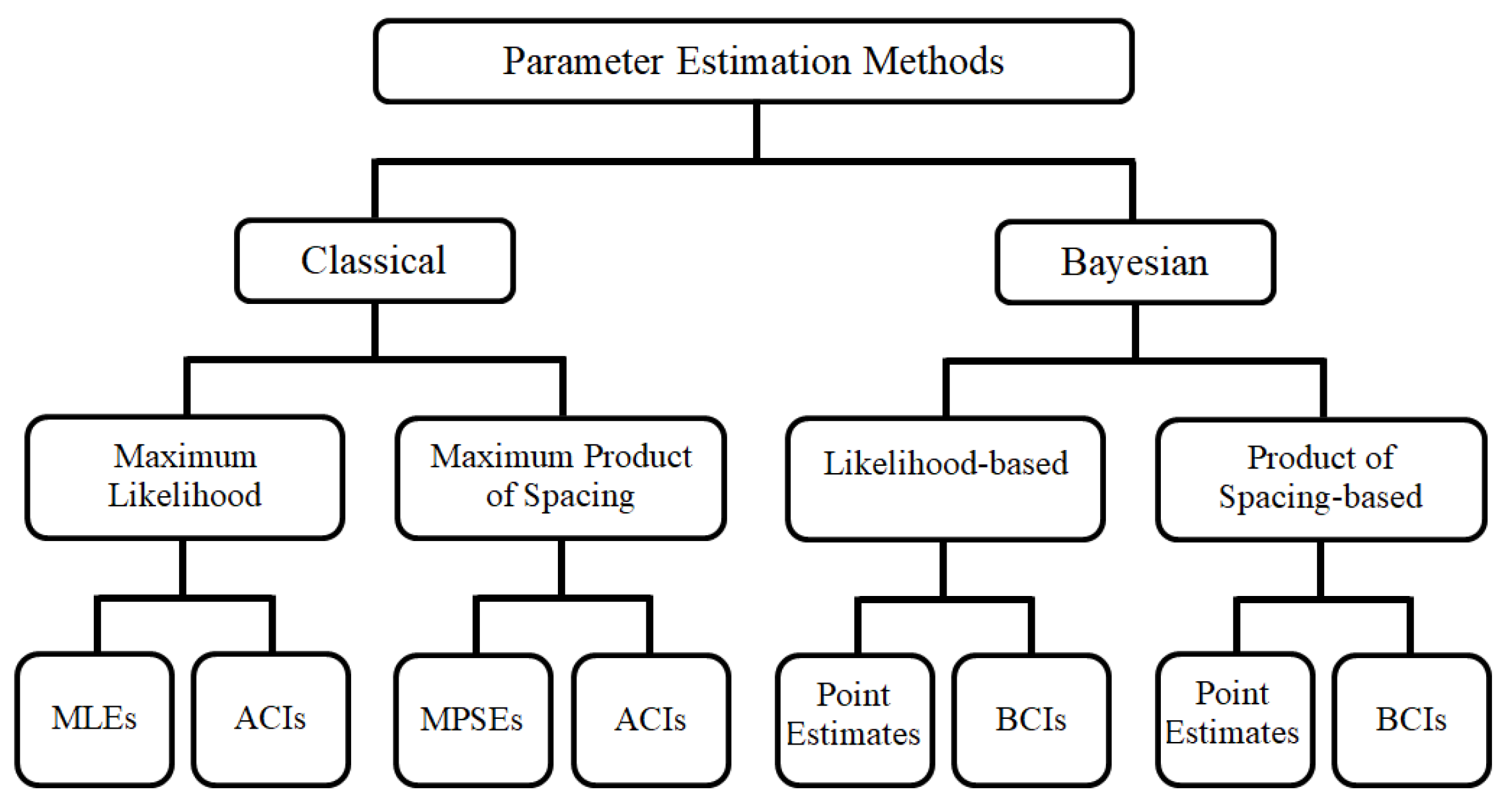
2. Model Description
3. Maximum Likelihood Estimation
4. Maximum Product of Spacing Estimation
5. Bayesian Estimation
5.1. Bayesian Estimation Using LF-based
- Step 1.
- Put and determine the start values as .
- Step 2.
- Generate from evaluated at , and .
- Step 3.
- Employ MH steps to obtain from with NPD .
- Step 4.
- Use MH steps to acquire from with NPD .
- Step 5.
- Set .
- Step 6.
- Redo steps 2–5 M times to obtain .
5.2. Bayesian Estimation Using PSF-Based
- Step 1.
- Set and determine the initial values as .
- Step 2.
- Generate from using the MH steps using .
- Step 3.
- Generate from using the MH steps using .
- Step 4.
- Generate from using the MH steps using .
- Step 5.
- Set .
- Step 6.
- Redo steps 2–5 M times to acquire .
6. Monte Carlo Simulations
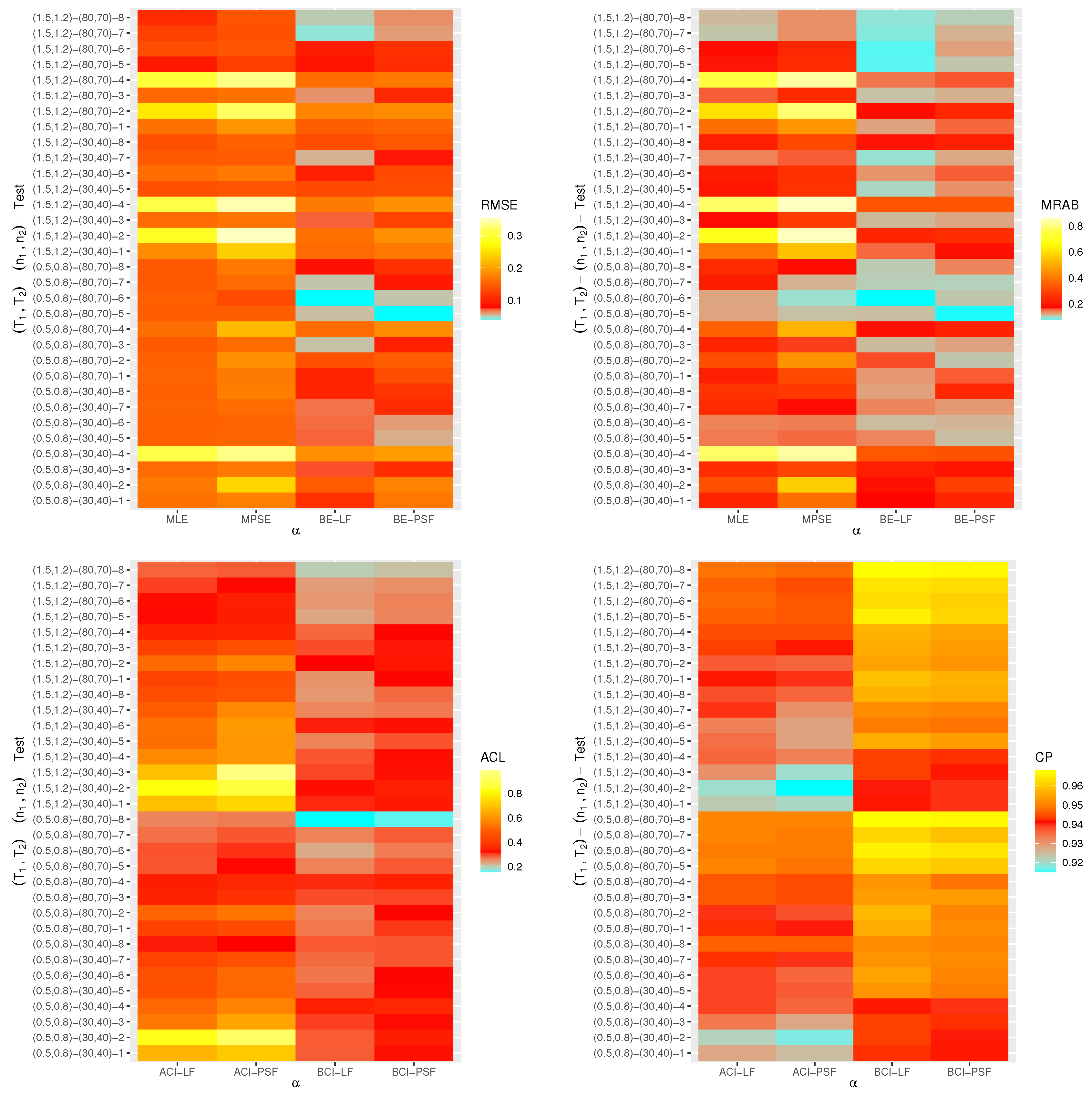
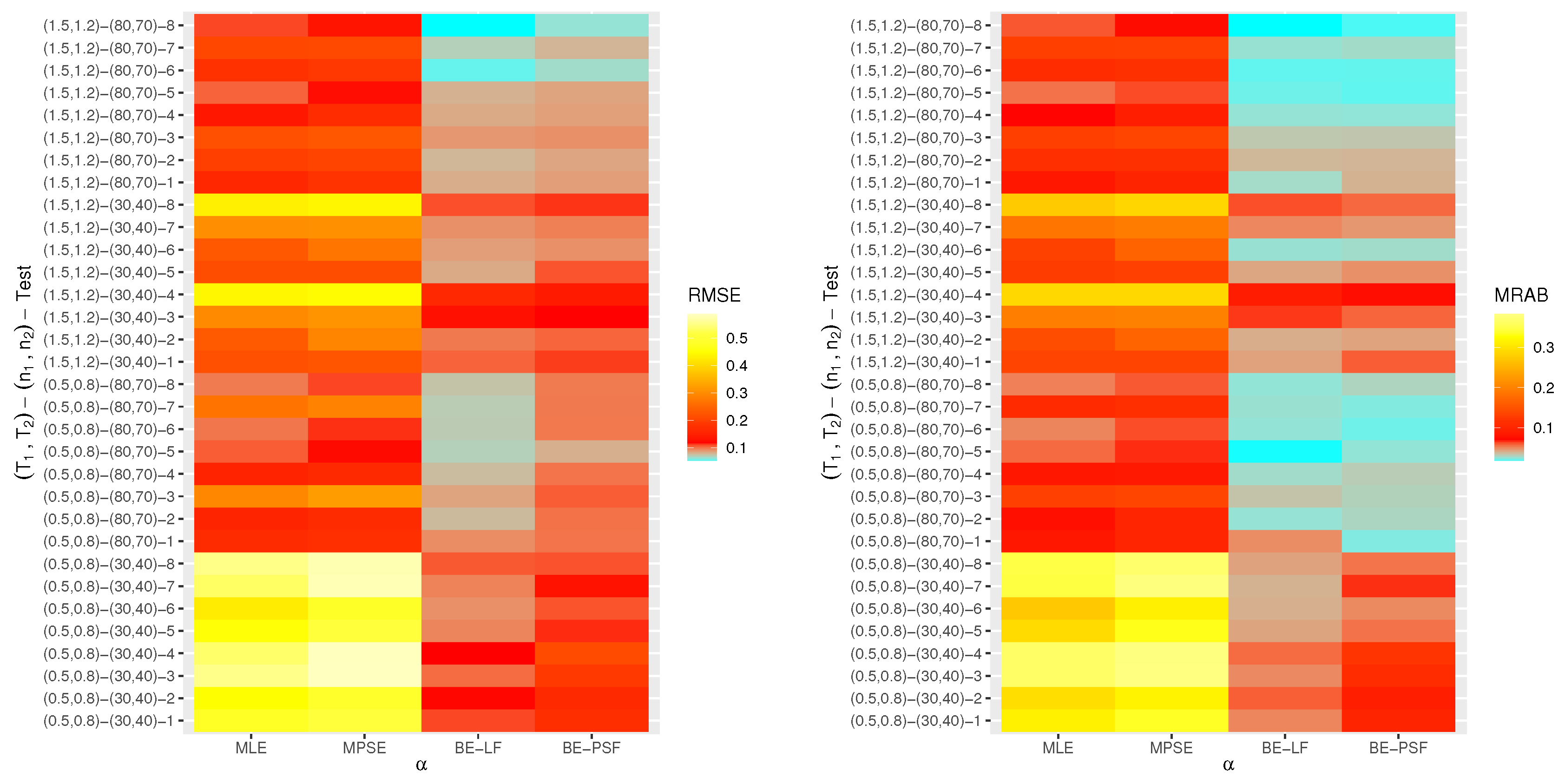
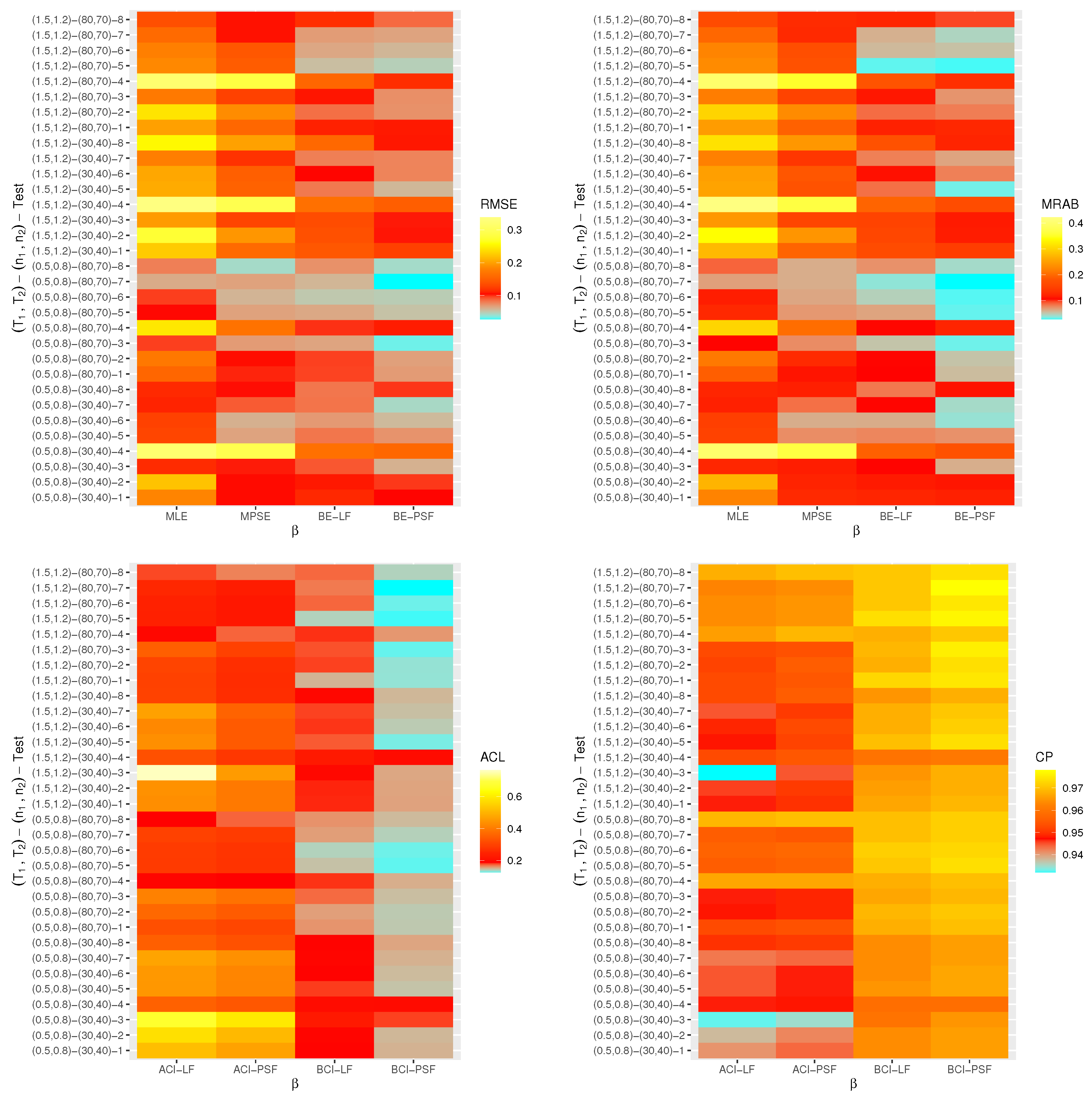
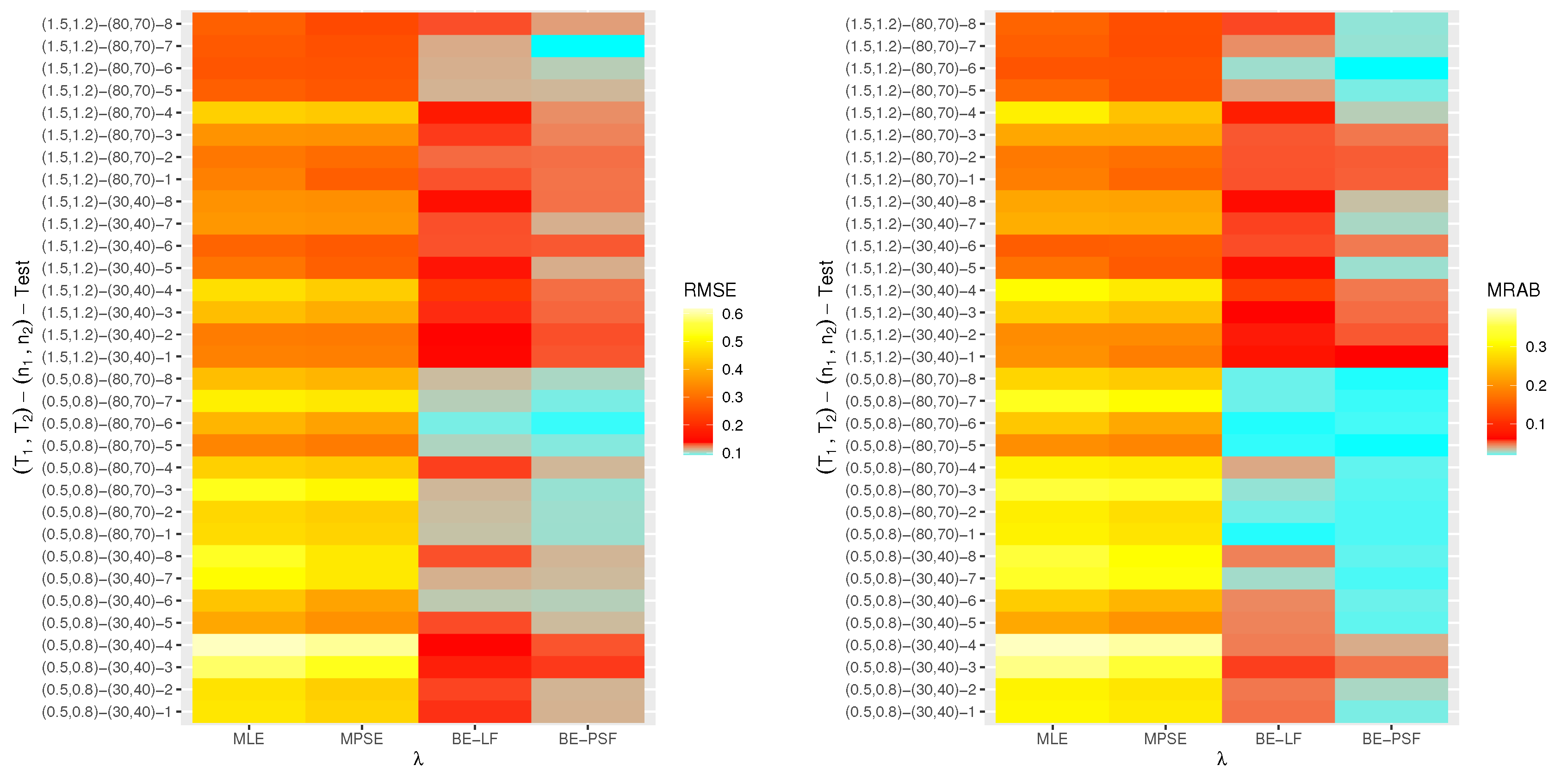
- The proposed point (or interval) estimates of , , and have shown good performance based on both given parameter sets.
- As (or ) increases, all suggested estimates function satisfactorily, which satisfies the consistency feature of the acquired estimates. Equivalent behavior is also noted when decrease.
- The Bayes estimates developed by LF-based (or PSF-based) methods provide higher performance compared to the frequentist estimates of all unknown parameters because the Bayesian point (or interval) estimates involve more priority information on the unknown parameters than the classical estimates.
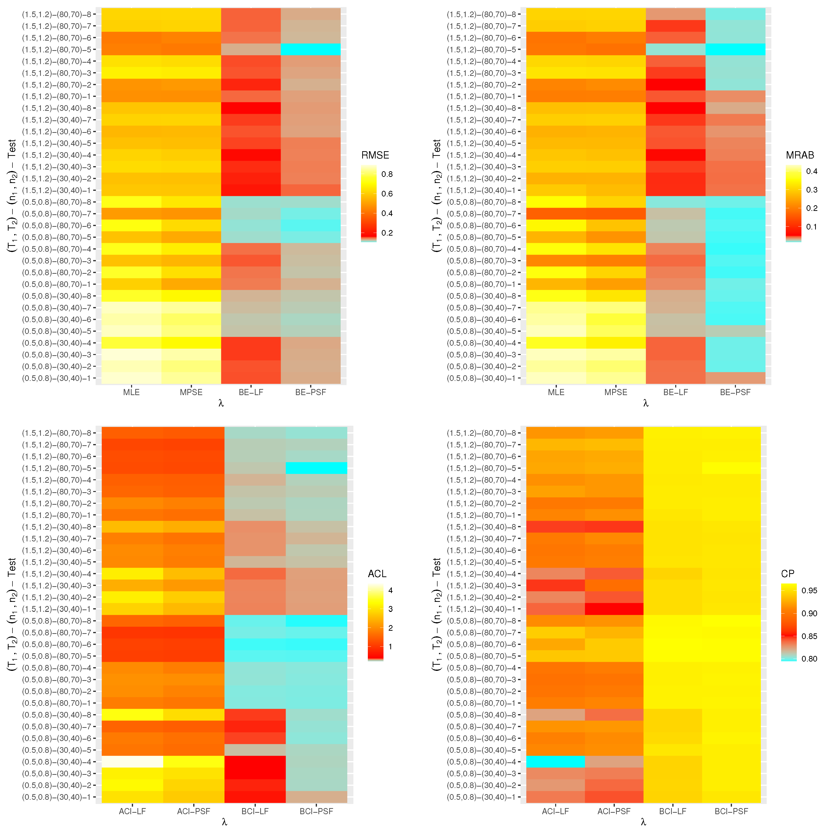
- The RMSEs and MRABs of all estimates of and grow as increase under Set 1, but those linked to the acceleration factor decrease (in the case of frequentist estimation) and increase (in the case of Bayesian estimation).
- The RMSEs and MRABs of all estimates for decrease, while those of grow as increase under Set 2. In the case of Set 1, the same pattern of as in Set 2 is shown.
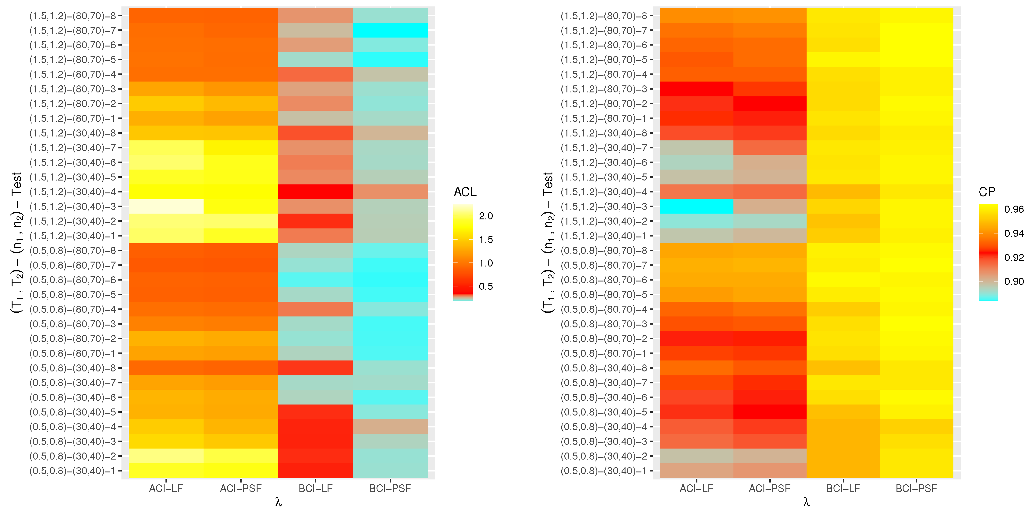
- The ACLs of all estimates of and grow, while those connected with decrease, and the opposite tendency is shown in terms of their CPs as increase under Set 1.
- As increase under Set 2, in most cases, the ACLs of and decrease (in the case of frequentist estimation) and increase (in the case of Bayesian estimation), while those associated with decrease based on all proposed methods. The opposite behavior is also observed in terms of their CPs.
- As increase, for each , the RMSEs, MRABs and ACLs of and increase, while those values associated with increase (in the case of frequentist estimation) and decrease (in the case of Bayesian estimation). Similarly, the opposite behavior is also noted in terms of their CPs.
- It is evident from comparing the four different estimation techniques, for both Sets 1 and 2, that the point/interval estimates of derived from the ML and BE-LF approaches behave better than the other estimates, while the estimates of and derived from the MPS and BE-PSF methods behave better than the other estimates.
- The point and interval estimates of the unknown parameters in the case of uniform (or left) censoring perform better than the others when comparing the effects of different progressive censoring plans.
- In conclusion, the simulation results suggested that the Bayes LF-based approach via the MH-within-Gibbs algorithm is the best for estimating the unknown shape parameter , while the Bayes PSF-based approach via the MH algorithm is the best for estimating the unknown parameters and .
7. Real Data Applications
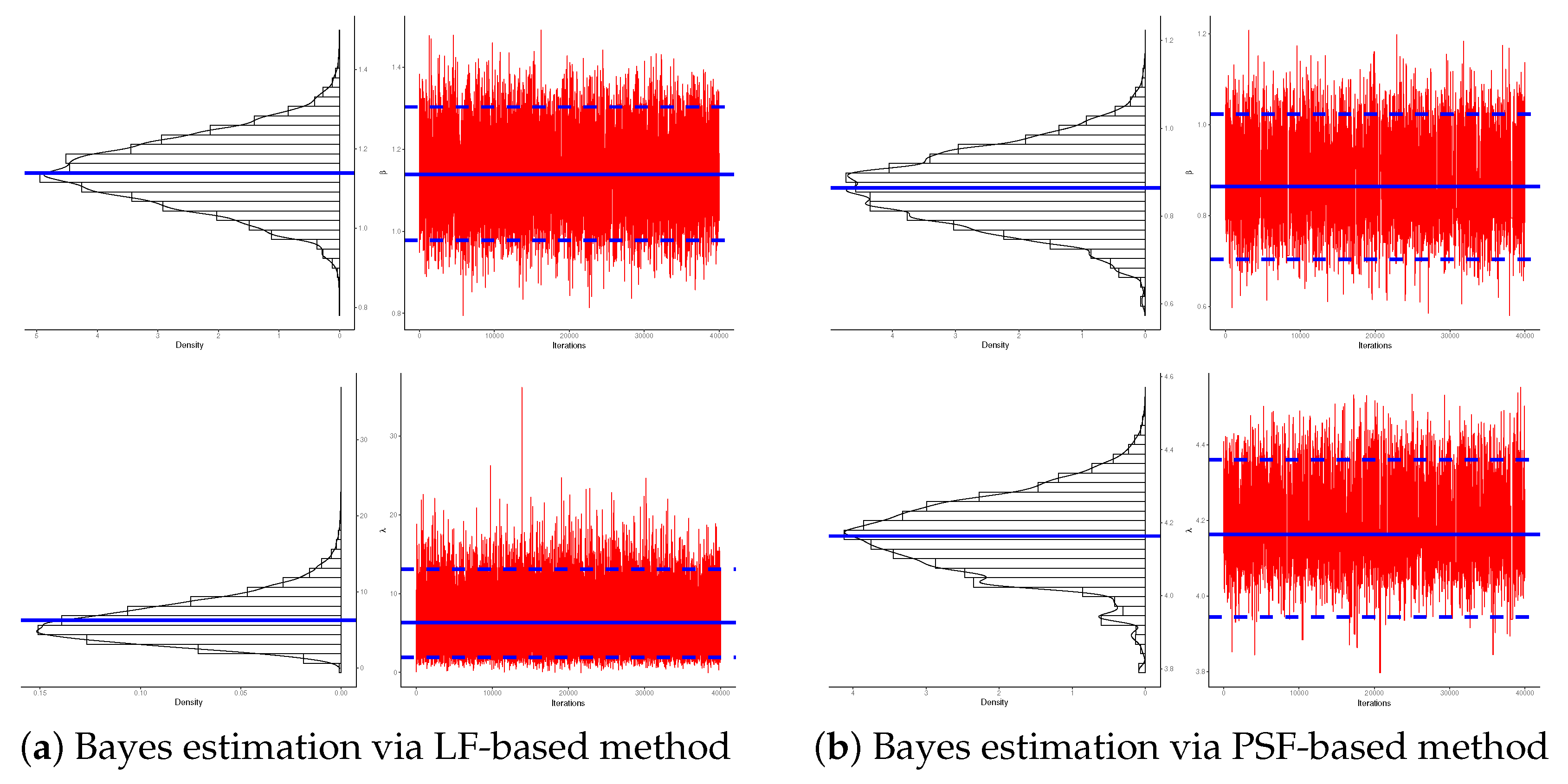
7.1. Micro-Droplets
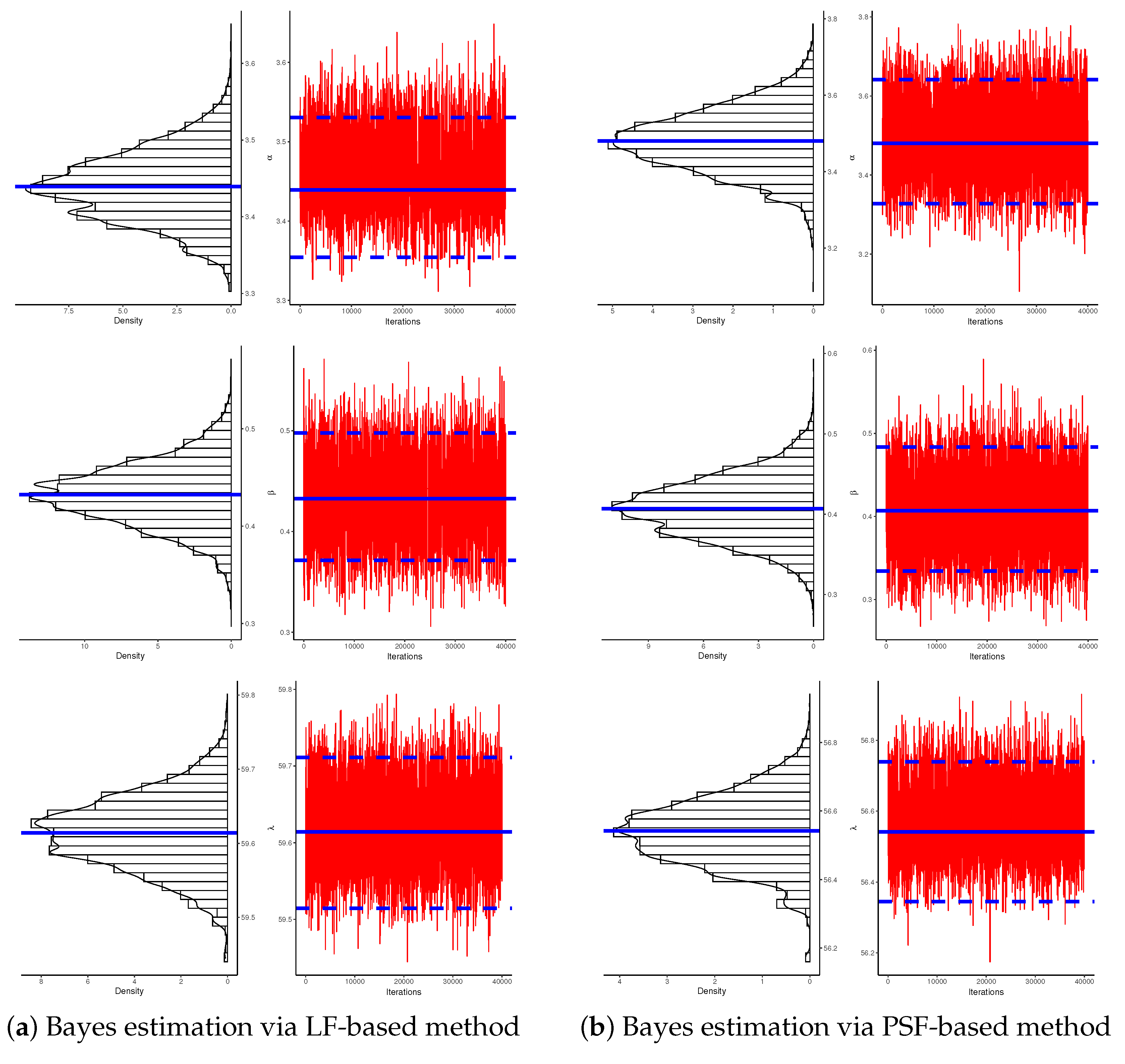
7.2. Light-Emitting Diodes
8. Concluding Remarks
Author Contributions
Funding
Institutional Review Board Statement
Informed Consent Statement
Data Availability Statement
Acknowledgments
Conflicts of Interest
References
- Ahmad, A.E.B.A.; Soliman, A.A.; Yousef, M.M. Bayesian estimation of exponentiated Weibull distribution under partially acceleration life tests. Bull. Malays. Math. Sci. Soc. 2016, 39, 227–244. [Google Scholar] [CrossRef]
- Dey, S.; Wang, L.; Nassar, M. Inference on Nadarajah–Haghighi distribution with constant stress partially accelerated life tests under progressive type-II censoring. J. Appl. Stat. 2022, 49, 2891–2912. [Google Scholar] [CrossRef]
- Wang, B.X.; Yu, K.; Sheng, Z. New inference for constant-stress accelerated life tests with Weibull distribution and progressively type-II censoring. IEEE Trans. Reliab. 2014, 63, 807–815. [Google Scholar] [CrossRef]
- Wang, L. Inference of constant-stress accelerated life test for a truncated distribution under progressive censoring. Appl. Math. Model. 2017, 44, 743–757. [Google Scholar] [CrossRef]
- El-Din, M.M.; Abd El-Raheem, A.M.; Abd El-Azeem, S.O. Inference for a constant-stress accelerated life testing for power generalized Weibull distribution under progressive type-II censoring. J. Stat. Appl. Probab. 2019, 8, 201–216. [Google Scholar]
- Dey, S.; Nassar, M. Classical methods of estimation on constant stress accelerated life tests under exponentiated Lindley distribution. J. Appl. Stat. 2020, 47, 975–996. [Google Scholar] [CrossRef]
- Sief, M.; Liu, X.; Abd El-Raheem, A.E.R.M. Inference for a constant-stress model under progressive type-I interval censored data from the generalized half-normal distribution. J. Stat. Comput. Simul. 2021, 91, 3228–3253. [Google Scholar] [CrossRef]
- Kumar, D.; Nassar, M.; Dey, S.; Alam, F.M.A. On estimation procedures of constant stress accelerated life test for generalized inverse Lindley distribution. Qual. Reliab. Eng. Int. 2022, 38, 211–228. [Google Scholar] [CrossRef]
- Abdel-Hamid, A.H.; AL-Hussaini, E.K. Estimation in step-stress accelerated life tests for the exponentiated exponential distribution with type-I censoring. Comput. Stat. Data Anal. 2009, 53, 1328–1338. [Google Scholar] [CrossRef]
- Hamada, M.S. Bayesian analysis of step-stress accelerated life tests and its use in planning. Qual. Eng. 2015, 27, 276–282. [Google Scholar] [CrossRef]
- Nassar, M.; Okasha, H.; Albassam, M. E-Bayesian estimation and associated properties of simple step–stress model for exponential distribution based on type-II censoring. Qual. Reliab. Eng. Int. 2021, 37, 997–1016. [Google Scholar] [CrossRef]
- Amleh, M.A.; Raqab, M.Z. Inference in simple step-stress accelerated life tests for type-II censoring Lomax data. J. Stat. Theory Appl. 2021, 20, 364–379. [Google Scholar] [CrossRef]
- Hyun, S.; Lee, J. Constant-stress partially accelerated life testing for log-logistic distribution with censored data. J. Stat. Appl. Probab. 2015, 4, 193–201. [Google Scholar]
- Ahmadini, A.A.H.; Mashwani, W.K.; Sherwani, R.A.K.; Alshqaq, S.S.; Jamal, F.; Miftahuddin, M.; Abbas, K.; Razaq, F.; Elgarhy, M.; Al-Marzouki, S. Estimation of Constant Stress Partially Accelerated Life Test for Frechet Distribution with Type-I Censoring. Math. Probl. Eng. 2021, 2021, 9957944. [Google Scholar] [CrossRef]
- Mohamed, N.M. Estimation on kumaraswamy-inverse weibull distribution with constant stress partially accelerated life tests. Appl. Math. Inf. Sci. 2021, 15, 503–510. [Google Scholar]
- Nassar, M.; Alam, F.M.A. Analysis of Modified Kies Exponential Distribution with Constant Stress Partially Accelerated Life Tests under Type-II Censoring. Mathematics 2022, 10, 819. [Google Scholar] [CrossRef]
- Lin, C.T.; Huang, Y.L. On progressive hybrid censored exponential distribution. J. Stat. Comput. Simul. 2012, 82, 689–709. [Google Scholar] [CrossRef]
- Lin, C.T.; Chou, C.C.; Huang, Y.L. Inference for the Weibull distribution with progressive hybrid censoring. Comput. Stat. Data Anal. 2012, 56, 451–467. [Google Scholar] [CrossRef]
- Ismail, A.A. Statistical inference for a step-stress partially-accelerated life test model with an adaptive Type-I progressively hybrid censored data from Weibull distribution. Stat. Pap. 2016, 57, 271–301. [Google Scholar] [CrossRef]
- Okasha, H.; Mustafa, A. E-Bayesian estimation for the Weibull distribution under adaptive type-I progressive hybrid censored competing risks data. Entropy 2020, 22, 903. [Google Scholar] [CrossRef]
- Nassar, M.; Dobbah, S.A. Analysis of reliability characteristics of bathtub-shaped distribution under adaptive Type-I progressive hybrid censoring. IEEE Access 2020, 8, 181796–181806. [Google Scholar] [CrossRef]
- Nelson, W.B. Applied Life Data Analysis; Wiley: New York, NY, USA, 1982. [Google Scholar]
- Cheng, R.C.H.; Amin, N.A.K. Estimating parameters in continuous univariate distributions with a shifted origin. J. R. Stat. Soc. B 1983, 45, 394–403. [Google Scholar] [CrossRef]
- Anatolyev, S.; Kosenok, G. An alternative to maximum likelihood based on spacings. Econ. Theory 2005, 21, 472–476. [Google Scholar] [CrossRef]
- Ng, H.K.T.; Luo, L.; Hu, Y.; Duan, F. Parameter estimation of three parameter Weibull distribution based on progressively Type-II censored samples. J. Stat. Comput. Simul. 2012, 82, 1661–1678. [Google Scholar] [CrossRef]
- Wang, S.; Chen, W.; Chen, M.; Zhou, Y. Maximum likelihood estimation of the parameters of the inverse Gaussian distribution using maximum rank set sampling with unequal samples. Math. Popul. Stud. 2021. [Google Scholar] [CrossRef]
- Basu, S.; Singh, S.K.; Singh, U. Bayesian inference using product of spacings function for progressive hybrid Type-I censoring scheme. Statistics 2018, 52, 345–363. [Google Scholar] [CrossRef]
- Basu, S.; Singh, S.K.; Singh, U. Estimation of inverse Lindley distribution using product of spacings function for hybrid censored data. Methodol. Comput. Appl. Probab. 2019, 21, 1377–1394. [Google Scholar] [CrossRef]
- Okasha, H.; Nassar, M. Product of spacing estimation of entropy for inverse Weibull distribution under progressive type-II censored data with applications. J. Taibah Univ. Sci. 2022, 16, 259–269. [Google Scholar] [CrossRef]
- Abushal, T.A.; Soliman, A.A. Estimating the Pareto parameters under progressive censoring data for constant-partially accelerated life tests. J. Stat. Comput. Simul. 2015, 85, 917–934. [Google Scholar] [CrossRef]
- Mahmoud, M.A.; El-Sagheer, R.M.; Abou-Senna, A.M. Estimating the Modified Weibull Parameters in Presence of Constant-Stress Partially Accelerated Life Testing. J. Stat. Theory Appl. 2018, 17, 242–260. [Google Scholar] [CrossRef] [Green Version]
- Coolen, F.P.A.; Newby, M.J. Bayesian estimation of location parameters in life distributions. Reliab. Eng. Syst. Saf. 1994, 45, 293–298. [Google Scholar] [CrossRef]
- Singh, U.; Singh, S.K.; Singh, R.K. Product spacings as an alternative to likelihood for Bayesian inferences. J. Stat. Appl. Probab. 2014, 3, 179–188. [Google Scholar] [CrossRef]
- Nassar, M.; Dey, S.; Wang, L.; Elshahhat, A. Estimation of Lindley constant-stress model via product of spacing with Type-II censored accelerated life data. Commun.-Stat.-Simul. Comput. 2021. [Google Scholar] [CrossRef]
- Henningsen, A.; Toomet, O. maxLik: A package for maximum likelihood estimation in R. Comput. Stat. 2011, 26, 443–458. [Google Scholar] [CrossRef]
- Plummer, M.; Best, N.; Cowles, K.; Vines, K. CODA: Convergence diagnosis and output analysis for MCMC. R News 2006, 6, 7–11. [Google Scholar]
- Gelman, A.; Rubin, D.B. Inference from Iterative Simulation Using Multiple Sequences. Stat. Sci. 1992, 7, 457–511. [Google Scholar] [CrossRef]
- Brooks, S.P.; Gelman, A. General Methods for Monitoring Convergence of Iterative Simulations. J. Comput. Graph. Stat. 1997, 7, 434–455. [Google Scholar]
- Aliabadi, A.A.; Rogak, S.N.; Green, S.I.; Bartlett, K.H. CFD simulation of human coughs and sneezes: A study in droplet dispersion, heat, and mass transfer. ASME Int. Mech. Eng. Congr. Expo. 2010, 44441, 1051–1060. [Google Scholar]
- Asadi, S.; Panahi, H.; Swarup, C.; Lone, S.A. Inference on adaptive progressive hybrid censored accelerated life test for Gompertz distribution and its evaluation for virus-containing micro droplets data. Alex. Eng. J. 2022, 61, 10071–10084. [Google Scholar] [CrossRef]


| Test | |||
|---|---|---|---|
| (30,40) | 1 | (15,20) | |
| 2 | |||
| 3 | |||
| 4 | |||
| 5 | (24,32) | ||
| 6 | |||
| 7 | |||
| 8 | |||
| (80,70) | 1 | (40,35) | |
| 2 | |||
| 3 | |||
| 4 | |||
| 5 | (64,56) | ||
| 6 | |||
| 7 | |||
| 8 |
| Normal use condition (0.35 m/s) | |||||||||
| 0.94 | 1.08 | 1.10 | 1.60 | 1.92 | 2.28 | 2.48 | 2.60 | 2.76 | 3.00 |
| 3.22 | 3.22 | 3.40 | 3.58 | 3.60 | |||||
| Accelerated stress condition (0.20 m/s) | |||||||||
| 1.60 | 1.80 | 1.94 | 2.02 | 2.18 | 2.30 | 2.30 | 2.30 | 2.36 | 2.44 |
| 2.50 | 2.54 | 2.58 | 2.60 | 2.62 | 2.68 | 2.72 | 2.74 | 2.80 | |
| Condition | Par. | MLE (SE) | KS (p-Value) |
|---|---|---|---|
| Normal use | 3.3465 (0.9741) | 0.2222 (0.449) | |
| 2.1103 (0.3994) | |||
| Accelerated stress | 85.363 (56.411) | 0.2323 (0.253) | |
| 5.7663 (0.9130) |
| Sample | Generated Data | |||
|---|---|---|---|---|
| 1 | 2.50(6) | 4 | 0.94, 1.08, 1.10, 1.60, 1.92, 2.48 | |
| 2.45(8) | 7 | 1.60, 1.80, 1.94, 2.02, 2.18, 2.30, 2.36, 2.44 | ||
| 2 | 3.10(9) | 3 | 0.94, 1.08, 1.10, 1.60, 1.92, 2.28, 2.48, 2.76, 3.00 | |
| 2.65(13) | 4 | 1.60, 1.80, 1.94, 2.02, 2.18, 2.30, 2.36, 2.44, 2.50, 2.54, 2.58, 2.60, 2.62 | ||
| 3 | 3.60(10) | 1 | 0.94, 1.08, 1.10, 1.60, 1.92, 2.28, 2.60, 3.00, 3.22, 3.58 | |
| 2.75(15) | 1 | 1.60, 1.80, 1.94, 2.02, 2.18, 2.30, 2.30, 2.30, 2.36, 2.44, 2.50, 2.54, 2.60, 2.68, 2.74 |
| Sample | Par. | MLE | BE-LF | ACI-LF | BCI-LF | ||||||
|---|---|---|---|---|---|---|---|---|---|---|---|
| MPSE | BE-PSF | ACI-PSF | BCI-PSF | ||||||||
| Est. | SE. | Est. | SE. | Lower | Upper | Length | Lower | Upper | Length | ||
| 1 | 5.5147 | 0.9999 | 5.3973 | 0.1516 | 3.5549 | 7.4745 | 3.9196 | 5.2100 | 5.5896 | 0.3796 | |
| 4.6872 | 0.8179 | 4.5855 | 0.1369 | 3.0841 | 6.2904 | 3.2063 | 4.4184 | 4.7714 | 0.3530 | ||
| 1.1620 | 0.2567 | 1.1390 | 0.0874 | 0.6589 | 1.6651 | 1.0062 | 0.9782 | 1.3031 | 0.3249 | ||
| 0.9410 | 0.2353 | 0.8639 | 0.1126 | 0.4797 | 1.4023 | 0.9225 | 0.7041 | 1.0234 | 0.3194 | ||
| 4.2236 | 2.3062 | 6.2978 | 3.5571 | 0.0000 | 8.7437 | 8.7437 | 1.8902 | 13.093 | 11.203 | ||
| 4.2622 | 2.3245 | 4.1635 | 0.1417 | 0.0000 | 8.8182 | 8.8182 | 3.9449 | 4.3603 | 0.4154 | ||
| 2 | 6.2496 | 1.1053 | 6.1308 | 0.1548 | 4.0833 | 8.4159 | 4.3326 | 5.9275 | 6.3234 | 0.3960 | |
| 5.3074 | 0.9784 | 5.2047 | 0.1378 | 3.3898 | 7.2251 | 3.8353 | 5.0369 | 5.3908 | 0.3539 | ||
| 1.3490 | 0.2274 | 1.3408 | 0.0798 | 0.9033 | 1.7947 | 0.8914 | 1.1857 | 1.4957 | 0.3101 | ||
| 1.1684 | 0.2182 | 1.1003 | 0.1033 | 0.7407 | 1.5961 | 0.8554 | 0.9427 | 1.2500 | 0.3074 | ||
| 4.9442 | 2.2856 | 9.0071 | 5.1519 | 0.4645 | 9.4239 | 8.9594 | 3.9441 | 16.253 | 12.309 | ||
| 4.7308 | 2.1924 | 4.6332 | 0.1401 | 0.4337 | 9.0279 | 8.5942 | 4.4238 | 4.8288 | 0.4050 | ||
| 3 | 6.2349 | 1.1476 | 6.1303 | 0.1434 | 3.9857 | 8.4841 | 4.4983 | 5.9373 | 6.3230 | 0.3857 | |
| 5.2030 | 1.8537 | 5.1008 | 0.1376 | 1.5699 | 8.8361 | 7.2663 | 4.9328 | 5.2878 | 0.3550 | ||
| 1.5898 | 0.2480 | 1.4999 | 0.1198 | 1.1038 | 2.0759 | 0.9722 | 1.3500 | 1.6569 | 0.3069 | ||
| 1.4036 | 0.3375 | 1.3322 | 0.1079 | 0.7420 | 2.0652 | 1.3232 | 1.1751 | 1.4889 | 0.3138 | ||
| 4.2551 | 1.8731 | 6.0161 | 3.7458 | 0.5839 | 7.9262 | 7.3423 | 1.2022 | 13.897 | 12.695 | ||
| 3.9316 | 2.1488 | 3.8345 | 0.1399 | 0.0000 | 8.1432 | 8.1432 | 3.6194 | 4.0297 | 0.4103 | ||
| Normal use condition |
| 0.18, 0.19, 0.19, 0.34, 0.36, 0.40, 0.44, 0.44, 0.45, 0.46, |
| 0.47, 0.53, 0.57, 0.57, 0.63, 0.65, 0.70, 0.71, 0.71, 0.75, |
| 0.76, 0.76, 0.79, 0.80, 0.85, 0.98, 1.01, 1.07, 1.12, 1.14, |
| 1.15, 1.17, 1.20, 1.23, 1.24, 1.25, 1.26, 1.32, 1.33, 1.33, |
| 1.39, 1.42, 1.50, 1.55, 1.58, 1.59, 1.62, 1.68, 1.70, 1.79, |
| 2.00, 2.01, 2.04, 2.54, 3.61, 3.76, 4.65, 8.97 |
| Accelerated stress condition |
| 0.13, 0.16, 0.20, 0.20, 0.21, 0.25, 0.26, 0.28, 0.28, 0.30, |
| 0.31, 0.33, 0.35, 0.35, 0.35, 0.39, 0.50, 0.52, 0.58, 0.60, |
| 0.60, 0.62, 0.63, 0.67, 0.71, 0.73, 0.75, 0.75, 0.78, 0.80, |
| 0.80, 0.86, 0.90, 0.91, 0.93, 0.93, 0.94, 0.98, 0.99, 1.01, |
| 1.03, 1.06, 1.06, 1.10, 1.22, 1.22, 1.24, 1.28, 1.39, 1.39, |
| 1.46, 1.48, 1.52, 1.74, 1.95, 2.46, 3.02, 5.16 |
| Condition | Par. | MLE (SE) | KS (p-Value) |
|---|---|---|---|
| Normal use | 0.5960 (0.0967) | 0.1189 (0.385) | |
| 1.3385 (0.1253) | |||
| Accelerated stress | 0.3709 (0.0718) | 0.1497 (0.149) | |
| 1.3563 (0.1305) |
| Sample | Generated Data | |||
|---|---|---|---|---|
| 1 | 1.55(25) | 4 | 0.18, 0.19, 0.34, 0.40, 0.45, 0.47, 0.53, 0.57, 0.63, 0.71, | |
| 0.75, 0.76, 0.79, 0.80, 0.85, 0.98, 1.01, 1.14, 1.15, 1.20, | ||||
| 1.26, 1.32, 1.33, 1.39, 1.50 | ||||
| 0.95(23) | 6 | 0.13, 0.16, 0.20, 0.25, 0.28, 0.28, 0.30, 0.31, 0.33, 0.35, | ||
| 0.39, 0.50, 0.52, 0.58, 0.60, 0.60, 0.62, 0.71, 0.75, 0.80, | ||||
| 0.80, 0.93, 0.94 | ||||
| 2 | 1.75(25) | 8 | 0.18, 0.19, 0.36, 0.44, 0.45, 0.47, 0.57, 0.63, 0.70, 0.71, | |
| 0.76, 0.79, 0.85, 1.01, 1.12, 1.15, 1.20, 1.24, 1.26, 1.33, | ||||
| 1.39, 1.50, 1.58, 1.62, 1.70 | ||||
| 1.25(24) | 10 | 0.13, 0.20, 0.21, 0.26, 0.28, 0.31, 0.35, 0.35, 0.50, 0.58, | ||
| 0.60, 0.63, 0.71, 0.75, 0.78, 0.80, 0.90, 0.93, 0.94, 0.99, | ||||
| 1.03, 1.06, 1.22, 1.24 | ||||
| 3 | 1.25(29) | 0 | 0.18, 0.19, 0.19, 0.34, 0.36, 0.40, 0.44, 0.44, 0.45, 0.46, | |
| 0.47, 0.53, 0.57, 0.57, 0.63, 0.65, 0.70, 0.71, 0.71, 0.75, | ||||
| 0.76, 0.76, 0.79, 0.80, 0.85, 0.98, 1.01, 1.14, 1.23 | ||||
| 0.95(29) | 0 | 0.13, 0.16, 0.20, 0.20, 0.21, 0.25, 0.26, 0.28, 0.28, 0.30, | ||
| 0.31, 0.33, 0.35, 0.35, 0.35, 0.39, 0.50, 0.52, 0.58, 0.60, | ||||
| 0.60, 0.62, 0.63, 0.67, 0.75, 0.78, 0.80, 0.86, 0.94 |
| Sample | Par. | MLE | BE-LF | ACI-LF | BCI-LF | ||||||
|---|---|---|---|---|---|---|---|---|---|---|---|
| MPSE | BE-PSF | ACI-PSF | BCI-PSF | ||||||||
| Est. | SE. | Est. | SE. | Lower | Upper | Length | Lower | Upper | Length | ||
| 1 | 3.5146 | 0.1635 | 3.4394 | 0.0879 | 3.1941 | 3.8352 | 0.6411 | 3.3543 | 3.5306 | 0.1763 | |
| 3.5368 | 0.1503 | 3.4803 | 0.0987 | 3.2422 | 3.8314 | 0.5892 | 3.3280 | 3.6414 | 0.3133 | ||
| 0.4510 | 0.0465 | 0.4326 | 0.0368 | 0.3598 | 0.5422 | 0.1824 | 0.3713 | 0.4977 | 0.1264 | ||
| 0.4141 | 0.0447 | 0.4069 | 0.0385 | 0.3266 | 0.5017 | 0.1751 | 0.3341 | 0.4834 | 0.1493 | ||
| 59.639 | 9.5397 | 59.614 | 0.0554 | 40.941 | 78.336 | 37.395 | 59.514 | 59.711 | 0.1968 | ||
| 56.640 | 2.1141 | 56.542 | 0.1396 | 52.497 | 60.784 | 8.2871 | 56.345 | 56.739 | 0.3948 | ||
| 2 | 1.2970 | 0.1776 | 1.3088 | 0.0740 | 0.9489 | 1.6450 | 0.6962 | 1.1695 | 1.4523 | 0.2827 | |
| 1.3067 | 0.1738 | 1.2539 | 0.0919 | 0.9661 | 1.6474 | 0.6813 | 1.1069 | 1.4047 | 0.2978 | ||
| 0.7949 | 0.0894 | 0.7687 | 0.0641 | 0.6197 | 0.9702 | 0.3505 | 0.6556 | 0.8844 | 0.2289 | ||
| 0.7282 | 0.0848 | 0.7050 | 0.0631 | 0.5619 | 0.8944 | 0.3325 | 0.5931 | 0.8214 | 0.2283 | ||
| 2.8352 | 0.8257 | 2.8734 | 0.6418 | 1.2169 | 4.4535 | 3.2367 | 1.7761 | 4.2653 | 2.4892 | ||
| 2.7867 | 0.7785 | 2.6833 | 0.1430 | 1.2609 | 4.3125 | 3.0516 | 2.4912 | 2.8778 | 0.3866 | ||
| 3 | 1.6269 | 0.1779 | 1.5894 | 0.0584 | 1.2782 | 1.9756 | 0.6975 | 1.5010 | 1.6776 | 0.1766 | |
| 1.6662 | 0.1389 | 1.6300 | 0.0816 | 1.3939 | 1.9384 | 0.5444 | 1.4882 | 1.7766 | 0.2884 | ||
| 0.7578 | 0.0741 | 0.7315 | 0.0448 | 0.6126 | 0.9031 | 0.2905 | 0.6612 | 0.8020 | 0.1408 | ||
| 0.7046 | 0.0677 | 0.6976 | 0.0486 | 0.5719 | 0.8373 | 0.2655 | 0.6045 | 0.7920 | 0.1875 | ||
| 15.993 | 4.9913 | 15.965 | 0.0573 | 6.2106 | 25.776 | 19.565 | 15.872 | 16.064 | 0.1929 | ||
| 15.024 | 2.1670 | 14.924 | 0.1419 | 10.777 | 19.271 | 8.4943 | 14.725 | 15.119 | 0.3946 | ||
Disclaimer/Publisher’s Note: The statements, opinions and data contained in all publications are solely those of the individual author(s) and contributor(s) and not of MDPI and/or the editor(s). MDPI and/or the editor(s) disclaim responsibility for any injury to people or property resulting from any ideas, methods, instructions or products referred to in the content. |
© 2023 by the authors. Licensee MDPI, Basel, Switzerland. This article is an open access article distributed under the terms and conditions of the Creative Commons Attribution (CC BY) license (https://creativecommons.org/licenses/by/4.0/).
Share and Cite
Nassar, M.; Elshahhat, A. Statistical Analysis of Inverse Weibull Constant-Stress Partially Accelerated Life Tests with Adaptive Progressively Type I Censored Data. Mathematics 2023, 11, 370. https://doi.org/10.3390/math11020370
Nassar M, Elshahhat A. Statistical Analysis of Inverse Weibull Constant-Stress Partially Accelerated Life Tests with Adaptive Progressively Type I Censored Data. Mathematics. 2023; 11(2):370. https://doi.org/10.3390/math11020370
Chicago/Turabian StyleNassar, Mazen, and Ahmed Elshahhat. 2023. "Statistical Analysis of Inverse Weibull Constant-Stress Partially Accelerated Life Tests with Adaptive Progressively Type I Censored Data" Mathematics 11, no. 2: 370. https://doi.org/10.3390/math11020370