Integral Models in the Form of Volterra Polynomials and Continued Fractions in the Problem of Identifying Input Signals

Abstract

The paper discusses the prospect of using a combined model based on finite segments (polynomials) of the Volterra integral power series. We consider a case when the problem of identifying the Volterra kernels is solved. The predictive properties of the classic Volterra polynomial are improved by adding a linear part in the form of an equivalent continued fraction. This technique allows us to distinguish an additional parameter—the connection coefficient $\alpha$, which is effective in adapting the constructed integral model to changes in technical parameters at the input of a dynamic system. In addition, this technique allows us to take into account the case of perturbing the kernel of the linear term of the Volterra polynomial in the metric $C[0,T]$ by a given value $\delta$, implying the ideas of Volterra regularizing procedures. The problem of choosing the connection coefficient is solved using a special extremal problem. The developed algorithms are used to solve the problem of identifying input signals of test dynamic systems, among which, in addition to mathematical ones, thermal power engineering devices are used.

1. Introduction

Present-day methods of mathematical modeling of nonlinear dynamic systems include extensive theoretical and algorithmic tools, including the Volterra functional integral power series, Wiener functional series, Hammerstein and Wiener–Hammerstein models, self-organization algorithms, genetic algorithms, and neural networks. In the theory of mathematical modeling of dynamic systems, methods are widespread that use, firstly, a priori information about the internal structure of the simulated objects, secondly, observed data on the behavior of the object under study and, finally, the joint use of information of the first and second types. An insufficiency of a priori data about the structure of the object of study, as a rule, lead researchers to use approaches that, on the one hand, take into account information about the object at the stage of constructing a mathematical model, for example, using a training sample, and on the other hand, carry out “adjustment” of parameters and formation of models based on both current and retrospective information directly when using the model [1].

To identify the dynamic characteristics of a nonlinear system under conditions of a priori uncertainty about the internal structure, various methods have been developed (see, for example, [2]), among which Volterra functional series occupy a worthy place.

In the scientific literature, see for example [3,4], the universal properties of the Volterra integral power series and their applicability for various technical objects are noted. The monograph ([5], p. 247) states that “analytical study of nonlinear systems using functional power series of the Volterra type is equivalent to the analysis of nonlinear systems using experimental data”.

Note that there are diametrically opposed points of view when assessing the effectiveness and relevance of this mathematical tool. In particular, in the monographs [3,6,7,8], this method seems quite promising, and in [9,10], the opposite point of view is presented. The strengths mentioned are, first of all, the applicability for various modes of the object under study and interaction with a wide class of technical systems. The weakness mentioned is the limitation of the degree of nonlinearity of the system. In the review ([11], p. 358), authors noted that, currently, the “Volterra series is mainly used for the analysis and modeling of nonlinear systems in the simulation or laboratory stage”. Therefore, the development of new methods for constructing Volterra integral models and their modifications still remains an urgent problem.

Constructing a model of nonlinear dynamics in the form of the Volterra polynomial

$$y\left(t\right)=\sum _{n=1}^N\underset{0}{\overset{t}{\int }}\dots \underset{0}{\overset{t}{\int }}{K}_n(s_1,\dots ,s_n)\prod _{i=1}^{n}x(t-s_i)d{s}_i,t\in [0,T],$$

(1)

consists of determining the required number of terms of the series (1) and estimating the Volterra kernels of the corresponding orders. Here, the functions $K_n$ (due to the scalarity of the input signal $x\left(t\right)$) are symmetric with respect to their variables $s_1,\dots ,s_n$. Authors, as a rule, use a segment of the Volterra series (polynomial) at $N=2,3$. The limitation to two or three terms is effective only in the case of weak nonlinearity, for example, when the input signals of the system are small.

If the amplitude (height) of the input signals is relatively large, then sufficient accuracy can only be ensured by a set of models built for certain domains of change in the input signals. As noted in [10], the kernels in (1) “become dependent on the approximation domain, i.e., on the levels and duration of the signals.” Thus, the effectiveness of using Volterra series depends on solving the problem of identifying the first two or three terms of the series (1) and, in addition, on algorithms for constructing integral models in real time.

One of the common ways to construct dynamic integral models is to move from (1) to the discrete form [12,13,14,15]:

$$y\left(t\right)=\sum _{n=1}^P\sum _{i_1=1}^L\cdots \sum _{i_n=1}^L{h}_n\left(i_1,\dots ,i_n\right)x(t-i_1)\dots x(t-i_n)+e\left(t\right),$$

(2)

where $h_n$ is a discrete analogue of the Volterra kernel, L is finite memory, P is the order of the polynomial, $e\left(t\right)$ is some error (noise). The ratio (2) is considered as a functional polynomial regression model (see, for example, [16,17,18]).

Constructing a Volterra regression model involves a number of difficulties. They are associated, in particular, with the choice of the number L, which determines the system memory, as well as with the presence of errors in the source data (as noted in [19], “the identification problem by the least squares method is one of the incorrect ones”). Therefore, it is no coincidence that research in this direction continues to the present day [20].

In practice, a situation of insufficient training data often arises. In a series of papers [21,22,23,24], a new method for solving the identification problem with small amounts of input and output data is considered, based on the introduction of randomized models in which parameters are treated as random variables.

The papers [23,24] propose a method for determining statistical dependencies between input and output data based on linear and power randomized models. Their construction involves estimating probabilistic characteristics. This approach was later developed in [21,22] to simulate a dynamic system, the output of which is measured with an error, using a randomized model of the form

$$y\left(t\right)=\sum _{n=1}^N\sum _{(s_1,\dots ,s_n)=0}^m{K}^{\left(n\right)}(s_1,\dots ,s_n)\prod _{i=1}^{n}x(t-s_i)+\xi \left(t\right),$$

where $t\in [m,m+l]$, l is the number of measurements, $s_i\in [0,m]$, $x\left(t\right)$ is the input (measured exactly), functions $K^{\left(n\right)}$ are random, $\xi \left(t\right)$ is random additive noise.

These approaches are based on the use of basic knowledge about the object at the preliminary training stage, which is performed during an active or passive experiment.

Among modern intelligent techniques of mathematical modeling of technological processes, there are known schemes for controlling algorithms for setting up models based on current data, i.e., the possibility of additional training of models during the functioning of dynamic systems and objects is provided [25]. This approach is characterized by taking into account all retrospective knowledge about the object, which leads to increased modeling accuracy. Models based on the Volterra integral power series (1) and their modifications have wide application possibilities in intelligent systems for modeling and controlling dynamic objects (see, for example, [26,27,28,29]). In this case, both tools for constructing an IT management infrastructure [27] and management principles of model predictive control [28,29] are used. In relation to (1), it is natural to perceive Volterra kernels as functions specified with some error. An additional parameter introduced into such a model will allow the response to be adjusted taking into account the current source data (input signals). Thus, the design of the modified Volterra polynomial should include, in addition to the transient characteristics (Volterra kernels), taking into account the range of test sets of input–output signals, an additional parameter that takes into account the deviation of the current signals from their previous values from the training set. In relation to (1), this idea can be implemented through a combination with continued fractions, the use of which makes it possible to apply the perturbation method and, thereby, take into account the stochastic nature of the dynamics of objects.

In recent decades, the tool for continued fractions has been actively developing in the field of studying their properties [30,31]. Issues of applied application of continued fractions for problems of structural-parametric identification of models of linear dynamic objects were considered in works [32,33,34]. In [34], to approximate a continuous transfer function based on the theory of continued fractions, the authors use the results of measurements of input and output influences. The stated topics also include work on fractional differentiation [35,36,37].

In this paper, we propose a technique for using continued fractions, which consists of replacing the linear integral term in (1) with its equivalent in the form of an associated continued fraction and choosing the connection coefficient using a special extremal problem. The results of implementing the proposed approach are presented for some dynamic systems, including the problem of modeling the response of an element of a heat exchange unit [38]. The contents of the paper include the following sections: Section 2 contains the statement of the problem, Section 3 considers the solution to the problem of identifying the parameter $\alpha$, Section 4 includes the solution to the problem of identifying input signals. Section 3 and Section 4 also present the results of computational experiments for test dynamic systems, including the heat exchanger element. Section 5 contains conclusions and future research directions.

2. Problem Statement

Consider a polynomial (1) with $N=2,3$, the right-hand side of which meets the smoothness requirements for carrying out calculations, $y\left(0\right)=0$, kernels $K_i$, $i=1,2,3$ are continuous functions, in addition, $K_1\left(t\right)\ne 0$, $t\in [0,T]$, ${\left(K_1\left(t\right)\right)}_t^{\prime }\in C[0,T]$.

Let the following inequality hold:

$$\alpha +\underset{0}{\overset{t}{\int }}{K}_1\left(s_1\right)x(t-s_1)d{s}_1\ne 0,$$

(3)

where $\alpha \ne 0$, for all $t\in [0,T]$. Using the idea of continued fractions, under assumption (3), it is easy to obtain

$${\displaystyle \frac{\alpha }{{\displaystyle 1-\frac{\underset{0}{\overset{t}{\int }}{K}_1\left(s_1\right)x(t-s_1)d{s}_1}{\alpha +\underset{0}{\overset{t}{\int }}{K}_1\left(s_1\right)x(t-s_1)d{s}_1}}}-\alpha .}$$

(4)

Reducing fraction (4) to a common denominator will give the first term in (1):

$$\underset{0}{\overset{t}{\int }}{K}_1\left(s_1\right)x(t-s_1)d{s}_1.$$

(5)

Thus, replacing (5) in (1) with the expression (4) gives the modified model

$${\displaystyle \frac{\alpha }{{\displaystyle 1-\frac{\underset{0}{\overset{t}{\int }}{K}_1\left(s_1\right)x(t-s_1)d{s}_1}{\alpha +\underset{0}{\overset{t}{\int }}{K}_1\left(s_1\right)x(t-s_1)d{s}_1}}}-\alpha +\sum _{n=2}^N\underset{0}{\overset{t}{\int }}\dots \underset{0}{\overset{t}{\int }}{K}_n(s_1,\dots ,s_n)\prod _{i=1}^{n}x(t-s_i)d{s}_i=y\left(t\right).}$$

(6)

Further, we assume that the problem of identifying Volterra kernels for constructing models of the form (1) and (6) has been solved. We introduce the integral operator ${\displaystyle \mathbf{K}x:=\underset{0}{\overset{t}{\int }}{K}_1\left(s_1\right)x(t-s_1)d{s}_1}$ and the perturbed operator $\tilde{\mathbf{K}}x$ in which instead of $K_1\left(s_1\right)$ a function ${\tilde{K}}_1\left(s_1\right)$ is known that deviates in the metric $C[0,T]$ from $K_1\left(s_1\right)$ by a given value $\delta$. We will use the standard conditions regarding the kernel $K_1$ indicated at the beginning of this Section and the notation ${\tilde{K}}_1\left(t\right)=K_1\left(t\right)+\delta$, where $\delta$ is small positive parameter. Extensive literature addresses the issues of numerical solution of integral Volterra equations, including under the conditions of a perturbed operator. An important part of this line of research is the results obtained by M.M. Lavrentiev, A.M. Denisov, and A.S. Apartsyn. Using ideas from [39,40], instead of (6), consider a model of the following form:

$${\displaystyle \frac{\alpha }{{\displaystyle 1-\frac{\underset{0}{\overset{t}{\int }}{\tilde{K}}_1\left(s_1\right)x(t-s_1)d{s}_1}{\alpha +\underset{0}{\overset{t}{\int }}{K}_1\left(s_1\right)x(t-s_1)d{s}_1}}}-\alpha +\sum _{n=2}^N\underset{0}{\overset{t}{\int }}\dots \underset{0}{\overset{t}{\int }}{K}_n(s_1,\dots ,s_n)\prod _{i=1}^{n}x(t-s_i)d{s}_i=y_N\left(t\right),}$$

(7)

where $y_N\left(t\right)$ is the response of the integral model for a fixed value $N\ge 2$ and a given value $\delta$, and the expression ${\displaystyle -\alpha +\delta \underset{0}{\overset{t}{\int }}x\left(s\right)ds\ne 0}$ holds.

Remark 1. 

We do not consider the case when, in (4), everywhere instead of $K_1\left(t\right)$ there is ${\tilde{K}}_1\left(t\right)$. This is because under the assumption (3) with respect to ${\tilde{K}}_1\left(t\right)$, it degenerates into

$$\underset{0}{\overset{t}{\int }}{\tilde{K}}_1\left(s_1\right)x(t-s_1)d{s}_1+\sum _{n=2}^N\underset{0}{\overset{t}{\int }}\dots \underset{0}{\overset{t}{\int }}{K}_n(s_1,\dots ,s_n)\prod _{i=1}^{n}x(t-s_i)d{s}_i=\tilde{y}\left(t\right),$$

and thus, the problem of selecting the associated parameter α, taking into account the deviation of the current indicators $(x\left(t\right),\tilde{y}\left(t\right))$ from their previous values from the training set, is excluded from consideration.

Assuming that a model of the form (7) is built for some fixed value N, consider the problem of finding an input signal $x\left(t\right)$ that corresponds to a known response $y_N\left(t\right)$. This formulation arises in connection with the construction of a nonlinear automatic control system for a technical object ([5], p. 242). Given $\alpha$, $y\left(t\right)$, $K_i(i=1,2,\dots ,n)$, ${\tilde{K}}_1\left(t\right)$ the Equation (7) is N-th power (polynomial) Volterra equation of the first kind with respect to $x\left(t\right)$.

Note that to construct a model of the form (7), in contrast to (6), it is necessary to additionally solve the problem for identification of parameter $\alpha$. We will pay special attention to this issue in the next section.

3. On Choosing the Parameter $\mathbf{\alpha }$

We emphasize that the choice of parameter $\alpha \ne 0$ is limited by conditions that ensure that the denominators in (4) and (7) differ from zero. These conditions preserve the arbitrariness in the choice of $\alpha$. At the same time, the residual between $y_{et}\left(t\right)$ and $y_N\left(t\right)$ depends on the choice of this parameter. Note that the choice of the value of the connected parameter $\alpha$ affects the predictive properties of the integral model (7) and, accordingly, the accuracy of the response under an arbitrary perturbation $\delta$. Let us denote the response of model (7) at a certain value of $\alpha$ by $y_N^{\alpha }\left(t\right)$.

We formulate the problem of optimal (in some natural sense) choice of value $\alpha$. We will take the absolute value of the residual between $y_{et}\left(t\right)$ and $y_N^{\alpha }\left(t\right)$ as the objective function for a fixed $\delta$:

$$\left|\epsilon \left(t\right)\right|=|y_{et}\left(t\right)-y_N^{\alpha }\left(t\right)|,$$

where $y_{et}\left(t\right)$ is the response of the dynamic object (or its simulation model). Selecting $x\left(t\right)$ from the feasible family of signals $X\left(t\right)$, we set the accuracy criterion (7) in the form

$$\underset{x\left(t\right)\in X\left(t\right)}{max}|y_{et}\left(t\right)-y_N^{\alpha }\left(t\right)|\to \underset{\alpha \in R}{min}.$$

In fact, the $\epsilon \left(t\right)$ is some function depending on the parameters t and $\alpha$, so that $\epsilon \left(t\right)=\overline{\epsilon }(\alpha ,t)$. Then, the problem of parametric identification of the connection coefficient $\alpha$ for construction (7) can be reduced to solving an extremal problem: find a value of ${\alpha }^{\ast }$ that provides the minimum of maximum values $|\overline{\epsilon }(\alpha ,t)|$ on the set of feasible $t\in [0,T]$, $\alpha \in R$, i.e.,

$${\alpha }^{\ast }=arg\underset{\alpha \in R}{min}\{\underset{t\in [0,T]}{max}|\overline{\epsilon }(\alpha ,t)\left|\right\}.$$

(8)

Thus, we formulated the optimization problem (8) to remove the arbitrariness in choosing the connected coefficient $\alpha$. Now, we consider its solution using the example of some dynamic system.

Example 1. 

Let us illustrate the solution to the problem (8) when describing the response of a heat exchange unit element [38,41]:

$$\Delta i\left(t\right)=\frac{{\lambda }_1{\lambda }_2}{{\lambda }_2-{\lambda }_1}\underset{0}{\overset{t}{\int }}\left(\Delta Q\left(\eta \right)-\frac{Q_0}{D_0}\Delta D\left(\eta \right)\right)\gamma (t,\eta )d\eta ,$$

(9)

$$\gamma (t,\eta )=e^{-{\lambda }_1\underset{0}{\overset{t}{\int }}D\left(\xi \right)d\xi }-e^{-{\lambda }_2\underset{0}{\overset{t}{\int }}D\left(\xi \right)dxi},$$

where t is time, s; D is substance consumption, kg/s; Q is total heat load, kW; ${\lambda }_1$, ${\lambda }_2$ are some constants; the symbol “Δ” is increment, for example, $D\left(t\right)=D_0+\Delta D\left(t\right)$; the index “0” denotes the initial parameters $D_0=0.16$ kg/s; $Q_0=100$ kW; $i_0=1059$ kJ/kg.

To select the time range $t\in [0,T]$, we use the recommendations of [41]. The methodological role of the model is also noted there (9).

Note that according to (9), the change in $\Delta i\left(t\right)$ linearly depends on the input signal $\Delta Q\left(t\right)$. Therefore, without loss of generality, in this section, when identifying the parameter $\alpha$ in (7), we consider the case when $\Delta Q\left(t\right)=0$. Then, in terms of the model (7) $y_{et}\left(t\right)=\Delta i\left(t\right)$, $x\left(t\right)=\Delta D\left(t\right)$. Let us limit ourselves to (7) $N=2$. The procedure for identifying Volterra kernels in (7), where $t\in [0,20]$, is implemented using the technique from [40], the height (amplitude) of test signals from the training set is $\beta =25\%D_0=$0.04.

Now, we present the results of a computational experiment to solve the problem of parametric identification $\alpha$. To illustrate the effectiveness of the proposed model (7), we choose the input signal $x\left(t\right)=\xi e\left(t\right)$, where $\xi \ne \beta$, $e\left(t\right)$ is the Heaviside function. Let the kernel $\tilde{K}\left(t\right)$ in (7) be specified with an error of $\delta =0.1$. The maximum of $|\overline{\epsilon }(\alpha ,t)|$ is achieved either inside the interval under study at point $t_1$: $0<t_1<T$, or on the right boundary $t_2=T$. The parameter $\alpha$ is selected from the matching condition

$$|\overline{\epsilon }(\alpha ,t_1)|=|\overline{\epsilon }(\alpha ,t_2)|.$$

(10)

In particular, for $\xi =0.041$, the value of ${\alpha }^{\ast }$ obtained by solving the problems (8) and (10) was $-2.20331$, while $t_1=4.42713$, $t_2=20$, and $t^{\ast }=13.38662$; so,

$$|\overline{\epsilon }(-2.20331,4.42713)|=|\overline{\epsilon }(-2.20331,20)|=7.42245,$$

$$|\overline{\epsilon }(-2.20331,13.38662)|=0.$$

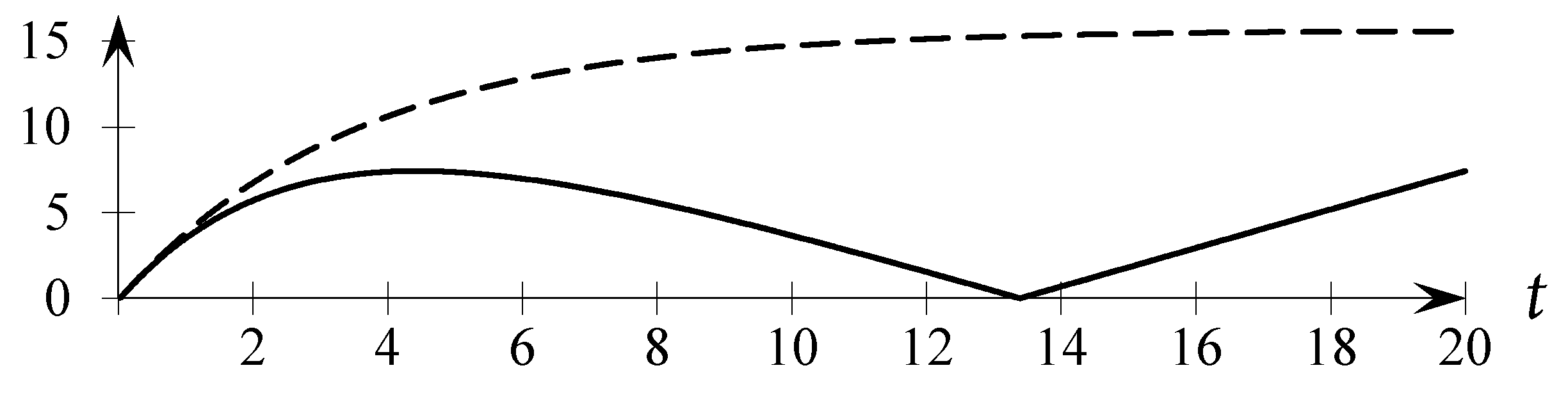
A comparison of the residuals $|\overline{\epsilon }({\alpha }^{\ast },t)|$ and $|y_{et}\left(t\right)-\tilde{y}\left(t\right)|$ is shown in Figure 1.

Figure 1. Graphs of functions $|\overline{\epsilon }({\alpha }^{\ast },t)|$ (solid line) and $|y_{et}\left(t\right)-\tilde{y}\left(t\right)|$ (dotted line).

The maximum values of response modeling errors (9) are reached at the end of the transient process, while

$$\underset{t\in [0,T]}{max}|y_{et}\left(t\right)-\tilde{y}\left(t\right)|=15.58662,\underset{t\in [0,T]}{max}|y_{et}\left(t\right)-y_2\left(t\right)|=7.42245,$$

$$\underset{0}{\overset{20}{\int }}|y_{et}\left(s\right)-\tilde{y}\left(s\right)|ds=257.7766,\underset{0}{\overset{20}{\int }}|y_{et}\left(s\right)-y_2\left(s\right)|ds=87.4427,$$

and the maximum relative application error (7) for the selected signal $x\left(t\right)=0.041$ is $1.2$%. Results of comparison of residuals $|\overline{\epsilon }({\alpha }^{\ast },T)|$ and $|y_{et}\left(T\right)-\tilde{y}\left(T\right)|$ for $\xi$ from the range $0.041÷0.045$ are given in Table 1.

Table 1. Results of a computational experiment for $\delta =0.1$.

$\mathit{\beta }$	${\mathit{\alpha }}^{\ast }$	$|{\mathit{y}}_{\mathbf{et}}\left(\mathit{T}\right)-\tilde{\mathit{y}}\left(\mathit{T}\right)|$	$|\overline{\mathit{\epsilon }}({\mathit{\alpha }}^{\ast },\mathit{T})|$
$0.041$	$-2.20331$	$15.58664$	$7.42245$
$0.042$	$-1.11759$	$31.17325$	$14.66873$
$0.043$	$-0.75644$	$46.75987$	$21.73701$
$0.044$	$-0.57593$	$62.34649$	$28.62992$
$0.045$	$-0.46761$	$77.93312$	$35.35023$

The table shows that the use of a modified model (7) involving the minimax problems (8) and (10) made it possible (for the selected range of technical characteristics) to reduce the modeling error by half.

Assuming further that a model of the form (7) has been constructed, let us consider the specifics of solving the polynomial equation that arises in the problem of reconstructing input signals.

4. On Identifying the Input Signal $\mathbf{x}\left(\mathbf{t}\right)$ in (7)

The theory and numerical methods for solving Volterra polynomial Equations (1) for $N=1$ and $N\ge 2$ have significant differences. In [42], it is shown that (1) for $N,\ge 2$ has a solution in the class of generalized functions. The publication [43] addresses further study of this issue. In this work, we will focus on studying the continuous solution to (7), $N\ge 2$.

In the works [41,44,45], there is a brief overview of the results of studies of polynomial Equations (1) for $N=2,3$, where $x\left(t\right)$ is a scalar function of time. Their most important feature is the locality of the solution in $C[0,T]$ (by locality we mean the smallness of the right end of the segment $\overline{t}<T$, where T cannot be replaced by a larger number). Since (1) has an exact solution only in special cases that correspond to $N=2,3$, let us dwell on the specifics of (7) for the indicated values of N.

Remark 2. 

The methodology for studying the continuous solution of Volterra polynomial Equations (1) and estimating the value of the parameter $\overline{t}$ is based on majorant estimates of special nonlinear integral inequalities introduced in [46,47]. These inequalities play the same role for (1) at a given $N>1$ as the Gronwall–Bellman inequality does for a linear Volterra equation of the first kind.

Let us move on to studying the Volterra polynomial equation of the first kind (7) ($N=2$). For simplicity, we choose the case of constant kernels $K_i\left(s\right)=k_i$, $k_i>0$, $i=1,2$. Without loss of generality, we set $k_1=1$, so that (7) for $N=2$, taking into account the notation, takes the form

$${\displaystyle \frac{\alpha }{{\displaystyle 1-\frac{(1+\delta )Q\left(t\right)}{\alpha +Q\left(t\right)}}}-\alpha +k_2{Q}^2\left(t\right)=y_2\left(t\right),}$$

(11)

where ${\displaystyle Q\left(t\right)=\underset{0}{\overset{t}{\int }}x\left(s\right)ds}$, $\alpha +Q\left(t\right)\ne 0$, $-\alpha +\delta Q\left(t\right)\ne 0$, $\delta >0$, $t\in [0,\overline{t}]$, $\alpha \in R$. In contrast to the quadratic polynomial Equation (1) for $N=2$, the Equation (11) ((7) for $N=2$) is cubic with respect to $Q\left(t\right)$. The exact solution (11)

$$Q^3\left(t\right)-\frac{\alpha }{\delta }{Q}^2\left(t\right)-\frac{y\left(t\right)\delta +\alpha (1+\delta )}{k_2\delta }Q\left(t\right)+\frac{y\left(t\right)\delta }{k_2\delta }=0$$

(12)

can be found by replacing the unknown in (12)

$$Q\left(t\right)=z\left(t\right)+\frac{\alpha }{3\delta }$$

and applying the Cardano formula [48] for the equation equivalent to (12)

$$z^3\left(t\right)+p\left(t\right)z\left(t\right)+q\left(t\right)=0,$$

(13)

where

$$p\left(t\right)=-\frac{y\left(t\right)+\alpha }{k_2}-\frac{\alpha }{k_2\delta }-\frac{{\alpha }^2}{3{\delta }^2},$$

$$q\left(t\right)=\frac{\alpha }{3k_2\delta }(2y\left(t\right)-\alpha )-\frac{1}{3}\frac{{\alpha }^2}{k_2{\delta }^2}-\frac{2}{27}\frac{{\alpha }^3}{{\delta }^3}.$$

Condition

$$D\left(t\right)=\frac{q^2\left(t\right)}{4}+\frac{p^3\left(t\right)}{27}\le 0,$$

guarantees the realness of the roots of (13). Thus, the critical value $\overline{t}$ is the smallest root of the equation $D\left(t\right)=0$$\forall t\ge 0$.

Let us illustrate the specifics of (11)–(13) with an example.

Example 2. 

Let the response of the dynamic system have the following form:

$$y_{et}\left(t\right)=\sum _{m=1}^{N_{et}}\frac{1}{m!}{\left(\underset{0}{\overset{t}{\int }}x\left(s\right)ds\right)}^m,N_{et}=3,t\in [0,T],T=1.$$

(14)

Applying the Volterra kernel identification technique for constructing (1) with $N=2$, as outlined in [40], we obtain

$$K_1\left(s_1\right)=1+\frac{s_1^2}{2},K_2(s_1,s_2)=\frac{1}{2}.$$

The response (7) to the signal $x\left(t\right)=e\left(t\right)$ is equal to $y_2\left(t\right)$, whence ${\displaystyle \overline{\epsilon }(\alpha ,t)=\frac{t\delta (\alpha +t+\frac{1}{6}{t}^3)}{\delta t-\alpha }}$. Solution to the problems (8), (10), in which ${\displaystyle y_2\left(t\right)=\frac{t\alpha (1+\frac{1}{6}{t}^3+\delta )}{\alpha -\delta t}+\frac{t^2}{2},t\in [0,T]}$, for a fixed $\delta =0.1$ is determined by the value $\alpha =-0.94048$. For definiteness, we choose the indicated values of $\delta$ and $\alpha$ and, for simplicity, limit ourselves to the case of constant kernels, choosing in (11)

$$k_1=\underset{0\le s_1\le 1}{min}|1+\frac{s_1^2}{2}|=1,k_2=\frac{1}{2}$$

and the desired right-hand side in the form $\frac{t^2}{2}+\frac{t^4}{8}-2t^3$.

Remark 3. 

Obviously, (14) is a partial sum of the series for the function ${\displaystyle exp\left(\underset{0}{\overset{t}{\int }}x\left(s\right)ds\right)}$. The choice of the value $k_1$ in this example is dictated by condition (12) from [47].

Note that even in the simplest case of constant kernels, the continuous solution to (1) for $N=2$, generally speaking, has a local character. The values $k_1$, $k_2$ are chosen to demonstrate this fact.

Besides, under the assumptions made, the solution to the polynomial Equation (1) is determined by the formula

$$x^{\ast }\left(t\right)=\frac{t(2-12t+t^2)}{\sqrt{4+4t^2-16t^3+t^4}}$$

for all $t\in [0,{\overline{t}}_1)$, where ${\overline{t}}_1=0.74036$. Moving on to the solution (1) with the perturbed kernel ${\tilde{k}}_1=k_1+\delta =1.1$, we have a solution $x^{\ast \ast }$ of the form

$$x^{\ast \ast }\left(t\right)=\frac{5t(2-12t+t^2)}{\sqrt{121+100t^2-400t^3+25t^4}}$$

for all $t\in [0,{\overline{t}}_2)$, where ${\overline{t}}_2=0.78241$. Here, ${\overline{t}}_1$ and ${\overline{t}}_2$ are the minimal positive roots of the equations $D_1=0$ and $D_2=0$, where $D_1$, $D_2$ is the corresponding expression under the radical. Using further Formulas (12) and (13) to solve (11), using the MAPLE computer system, we obtain that the real root of (11) $x^{\ast \ast \ast }\left(t\right)$ can be found for all $t\in [0,{\overline{t}}_3)$, where ${\overline{t}}_3=0.86210$. At the same time, by decreasing the value of $\alpha$, the value of ${\overline{t}}_3$ decreases, approaching the value of ${\overline{t}}_2$. In particular, when choosing $\alpha =-{10}^4$, ${\overline{t}}_3=0.78241$ coincides with ${\overline{t}}_2$ up to the fifth decimal place.

Let us present the results of a computational experiment, comparing the values of the roots of polynomial equations at the nodes $t_i=0.1÷0.9$. We use the symbol ${\ast }_j$$(j=1,2,3)$ to mark situations where the inequalities $t_i<{\overline{t}}_j$, which guarantee the realness of the roots, are violated.

Table 2 shows (see the second and third columns) that the influence of the error boundary layer is reflected in the values of $x^{\ast }\left(t_i\right)$, $x^{\ast \ast }\left(t_i\right)$ at $t_i=0.7$. Since in this example ${\overline{t}}_3>{\overline{t}}_2>{\overline{t}}_1$, the boundary layer affects the value of $x^{\ast \ast \ast }\left(t_i\right)$ at $t=0.8$. Comparing the value in the third and fourth columns of the table for $t_i=0.1÷0.6$, we can conclude that the solutions to Equations (1) and (11) and with perturbed kernel ${\tilde{k}}_1$ are quite close to each other.

Table 2. Values $x^{\ast }$, $x^{\ast \ast }$, $x^{\ast \ast \ast }$.

${\mathit{t}}_{\mathit{i}}$	${\mathit{x}}^{\ast }\left({\mathit{t}}_{\mathit{i}}\right)$	${\mathit{x}}^{\ast \ast }\left({\mathit{t}}_{\mathit{i}}\right)$	${\mathit{x}}^{\ast \ast \ast }\left({\mathit{t}}_{\mathit{i}}\right)$
$0.1$	$0.04038$	$0.03673$	$0.03675$
$0.2$	$-0.03585$	$-0.03261$	$-0.03264$
$0.3$	$-0.22833$	$-0.20728$	$-0.20696$
$0.4$	$-0.55337$	$-0.49882$	$-0.49419$
$0.5$	$-1.07143$	$-0.94914$	$-0.92311$
$0.6$	$-1.99749$	$-1.68974$	$-1.57229$
$0.7$	$-4.90247$	$-3.32067$	$-2.68428$
$0.8$	${\ast }_1$	${\ast }_2$	$-5.57908$
$0.9$	${\ast }_1$	${\ast }_2$	${\ast }_3$

It should be noted that the transition to (7) at $N=3$ involves the use of the Ferrari method and requires separate consideration.

5. Conclusions

The paper discusses the problem of modeling nonlinear dynamics using Volterra polynomials, associated with the problem of identifying input signals of a dynamic system. The approach proposed by the authors makes it possible to generate a modified integral model in a certain vicinity of the technical range of input influences. The formation of a modified model is based on the use of the tool of continued fractions and the subsequent solving an extremal problem of a special type to identify the associated parameter. Computational experiments have shown the effectiveness of a new type of integral model in describing nonlinear dynamics. The results of solving the problem of identifying input signals on a dynamic test system are comparable in accuracy to those discussed earlier in [45]. In addition, the use of modified integral models made it possible to expand the range of existence of a solution to a multilinear integral equation. This result was obtained experimentally (see Table 2) and requires further theoretical research.

References

- Bakhtadze, N.N. Virtual Analyzers: Identification Approach. Autom. Remote Control 2004, 65, 1691–1709. [Google Scholar] [CrossRef]
- Giannakis, G.B.; Serpedin, E. A bibliography on nonlinear system identification. Signal Process. 2001, 81, 533–580. [Google Scholar] [CrossRef]
- Volkov, N.V. Functional Series in Problems of Dynamics of Automated Systems; Janus-K: Moscow, Russia, 2001. (In Russian) [Google Scholar]
- Tsibizova, T.Y. Methods for identifying nonlinear control systems. Mod. Probl. Sci. Educ. 2015, 1–1, 109–116. (In Russian) [Google Scholar]
- Solodovnikov, V.V. (Ed.) Technical Cybernetics. Theory of Automatic Control; Mashinostroenie: Moscow, Russia, 1969; Volume 2. (In Russian) [Google Scholar]
- Venikov, V.A.; Sukhanov, O.A. Cybernetic Models of Electrical Systems; Energoizdat: Moscow, Russia, 1982. (In Russian) [Google Scholar]
- Danilov, L.V.; Mathanov, P.N.; Fillipov, E.S. Theory of Nonlinear Electrical Circuits; Energoizdat: Leningrad, Russia, 1990. (In Russian) [Google Scholar]
- Deich, A.M. Methods for Identifying Dynamic Objects; Energya: Moscow, Russia, 1979. (In Russian) [Google Scholar]
- Pupkov, K.A.; Shmykova, N.A. Analysis and Calculation of Nonlinear Systems Using Functional Power Series; Mashinostroenie: Moscow, Russia, 1989. (In Russian) [Google Scholar]
- Bobreshov, A.M.; Mymrikova, N.N. The problems of strongly nonlinear analysis for electron circuits based on Volterra series. Proc. Voronezh State Univ. Ser. Phys. Math. 2013, 2, 15–25. (In Russian) [Google Scholar]
- Cheng, C.M.; Peng, Z.K.; Zhang, W.M.; Meng, G. Volterra-series-based nonlinear system modeling and its engineering applications: A state-of-the-art review. Mech. Syst. Signal Process. 2017, 87, 340–364. [Google Scholar] [CrossRef]
- Alper, P. Consideration of the Discrete Volterra Series. IEEE Trans. Atom. Control 1965, 10, 322–327. [Google Scholar] [CrossRef]
- Schreues, D.; Schreues, D.; O’Droma, M.; Goacher, A.A.; Gadringer, M. RF Power Amplifier Be havioral Modeling; Cambrige University Press: Cambrige, UK, 2008. [Google Scholar]
- Wang, T.; Brazil, T.J. Volterra-Mapping-Based Behavioral Modeling of Nonlinear Circuitsand Systems for High Frequencies. IEEE Trans. Microw. Theory Tech. 2007, 51, 1433–1440. [Google Scholar] [CrossRef]
- Zhu, Q.; Dooley, J.; Brazil, T.J. Simplified Volterra Series Based Behavioral Modeling of RF Power Amplifiers Using Deviation—Reduction. In Proceedings of the 2006 IEEE MTT-S International Microwave Symposium Digest, San Francisco, CA, USA, 11–16 June 2006; pp. 1113–1116. [Google Scholar]
- Fatuev, V.A.; Khrapova, A.G. D-optimal sequential identification procedure for the dynamic Volterra regression model. Eurasian Union Sci. 2015, 4, 20–24. (In Russian) [Google Scholar]
- Franz, M.; Schölkopf, B. A unifying view of Wiener and Volterra theory and polynomial kernel regression. Neural Comput. 2006, 18, 3097–3118. [Google Scholar] [CrossRef]
- Kekatos, V.; Giannakis, G.B. Sparse Volterra and polynomial regression models: Recoverability and estimation. IEEE Trans. Signal Process. 2011, 59, 5907–5920. [Google Scholar] [CrossRef]
- Kapalin, V.I.; Popovich, D.E.; Kyong, N.M. Nonparametric identification of objects and solution of Volterra integral equations of the first order. Sci. Bull. Belsu. Ser. Comput. Sci. Appl. Math. 2006, 2, 37–41. (In Russian) [Google Scholar]
- Chinarro, D. System Identification Techniques. In System Engineering Applied to Fuenmayor Karst Aquifer (San Julian de Banzo, Huesca) and Collins Glacier (King George Island, Antarctica); Springer: Berlin/Heidelberg, Germany, 2014; pp. 11–51. [Google Scholar]
- Popkov, A.Y.; Popkov, Y.S. Parametric and nonparametric estimation for characteristics of randomized models under limited data (entropy approach). Math. Mod. 2015, 27, 63–85. (In Russian) [Google Scholar]
- Popkov, Y.S.; Popkov, A.Y.; Lysak, Y.N. Estimating the characteristics of randomized dynamic data models (the entropy-robust approach). Autom. Remote Control 2014, 75, 872–879. [Google Scholar] [CrossRef]
- Popkov, Y.S.; Popkov, A.Y.; Lysak, Y.N. Estimation of characteristics of randomized static models of data (entropy-robust approach. Autom. Remote Control 2013, 74, 1863–1877. [Google Scholar] [CrossRef]
- Popkov, Y.S.; Popkov, A.Y. Robust entropic estimation of randomized data models. Proc. Inst. Syst. Anal. Ras 2012, 62, 38–44. (In Russian) [Google Scholar]
- Bakhtadze, N.; Chereshko, A.; Elpashev, D.; Suleykin, A.; Purtov, A. Predictive associative models of processes and situations. IFAC-PapersOnLine 2022, 55, 19–24. [Google Scholar] [CrossRef]
- Popkov, Y.S. Controlled Positive Dynamic Systems with an Entropy Operator: Fundamentals of the Theory and Applications. Mathematics 2021, 9, 2585. [Google Scholar] [CrossRef]
- Pavlenko, V.; Shamanina, T. Application Volterra Model of the Oculo-Motor System for Personal Identification. In Proceedings of the 2022 IEEE 3rd KhPI Week on Advanced Technology (KhPIWeek), Kharkiv, Ukraine, 3–7 October 2022; pp. 1–6. [Google Scholar]
- Medina-Ramos, C.; Carbonel-Olazabal, D.; Betetta-Gomez, J.; Tafur-Anzualdo, I. Global Temperature Anomaly by Volterra-Laguerre Model from CO2 Emission, Solar Irradiance, Population, and the Oceans Heat Content. In Proceedings of the IEEE Biennial Congress of Argentina (ARGENCON), San Juan, Argentina, 7–9 September 2022; pp. 1–8. [Google Scholar]
- Medina-Ramos, C.; Betetta-Gomez, J.; Carbonel-Olazabal, D.; Pilco-Barrenechea, M. System identification and MPC based on the Volterra-Laguerre model for improvement of the laminator systems performance. In Proceedings of the 2013 IEEE International Symposium on Sensorless Control for Electrical Drives and Predictive Control of Electrical Drives and Power Electronics (SLED/PRECEDE), Munich, Germany, 17–19 October 2013; pp. 1–8. [Google Scholar]
- Waadeland, H.; Lorentzen, L. Continued Fractions with Applications; Springer: Berlin/Heidelberg, Germany, 2008. [Google Scholar]
- Cuyt, A.; Petersen, V.; Verdonk, B.; Waadeland, H.; Jones, W.B. Handbook of Continued Fractions for Special Functions; Springer: Berlin/Heidelberg, Germany, 2008. [Google Scholar]
- Kartashov, V.Y.; Novosel’tseva, M.A. Structural-and-parametric identification of linear stochastic plants using continuous fractions. Autom. Remote Control 2010, 71, 1727–1740. [Google Scholar] [CrossRef]
- Novoseltseva, M.A.; Gutova, S.G.; Kazakevich, I.A. Structural and Parametric Identification of a Multisinusoidal Signal Model by Using Continued Fractions. In Proceedings of the 2018 International Russian Automation Conference (RusAutoCon), Sochi, Russia, 9–16 September 2018; pp. 1–5. [Google Scholar]
- Novoseltseva, M.A.; Gutova, S.G.; Kagan, E.S.; Borodulin, D.M. Structural and parametric identification of the process model using a rotary pulsation machine. Tomsk State Univ. J. Control Comput. Sci. 2019, 49, 63–72. (In Russian) [Google Scholar] [CrossRef]
- Li, P.; Peng, X.; Xu, C.; Han, L.; Shi, S. Novel extended mixed controller design for bifurcation control of fractional-order Myc/E2F/miR-17-92 network model concerning delay. Math. Methods Appl. Sci. 2023, 1–21. [Google Scholar] [CrossRef]
- Jin, T.; Yang, X. Monotonicity theorem for the uncertain fractional differential equation and application to uncertain financial market. Math. Comput. Simul. (MATCOM) 2021, 190, 203–221. [Google Scholar] [CrossRef]
- Jin, T.; Xia, H. Lookback option pricing models based on the uncertain fractional-order differential equation with Caputo type. J. Ambient. Intell. Humaniz. Comput. 2021, 14, 6435–6448. [Google Scholar] [CrossRef]
- Tairov, E.A. Nonlinear modeling of heat transfer dynamics in a channel with a single-phase coolant. Proc. Acad. Sci. USSR Energy Transp. 1989, 1, 150–156. (In Russian) [Google Scholar]
- Lavrentiev, M.M. Some Improperly Posed Problems in Mathematical Physics; Springer: Berlin/Heidelberg, Germany, 1967. [Google Scholar]
- Apartsyn, A.S. Nonclassical linear Volterra Equations of the First Kind; VSP: Utrecht, The Netherlands, 2003. [Google Scholar]
- Solodusha, S.V.; Bulatov, M.V. Integral equations related to Volterra series and inverse problems: Elements of theory and applications in heat power engineering. Mathematics 2021, 9, 1905. [Google Scholar]
- Apartsyn, A.S. On the theory of multilinear Volterra equations of the first kind. Optim. Control Intell. 2005, 1, 5–27. (In Russian) [Google Scholar]
- Sidorov, N.A.; Sidorov, D.N. Generalized solutions to integral equations in the problem of identification of nonlinear dynamic models. Autom. Remote Control 2009, 70, 598–604. [Google Scholar] [CrossRef]
- Solodusha, S.V.; Grazhdantseva, E.Y. Test polynomial Volterra equation of the first kind in the problem of input signal identification. Tr. Instituta Mat. Mekhaniki Uro Ran 2021, 27, 161–174. (In Russian) [Google Scholar]
- Solodusha, S.; Suslov, K. An Approach to Stabilizing the Dynamic Loads of a Wind Turbine Generator Based on the Control of the Blades Setting Angle. IFAC-PapersOnLine 2022, 55, 76–80. [Google Scholar] [CrossRef]
- Apartsyn, A.S. Multilinear Volterra equations of the first kind. Autom. Remote Control 2004, 2, 263–269. [Google Scholar] [CrossRef]
- Apartsyn, A.S. Multilinear Volterra equations of the first kind and some problems of control. Autom. Remote Control 2008, 4, 545–558. [Google Scholar] [CrossRef]
- Mishina, A.P.; Proskuryakov, I.V. Higher Algebra; Fizmatgiz: Moscow, Russia, 1962. [Google Scholar]
Disclaimer/Publisher’s Note: The statements, opinions and data contained in all publications are solely those of the individual author(s) and contributor(s) and not of MDPI and/or the editor(s). MDPI and/or the editor(s) disclaim responsibility for any injury to people or property resulting from any ideas, methods, instructions or products referred to in the content. |
© 2023 by the authors. Licensee MDPI, Basel, Switzerland. This article is an open access article distributed under the terms and conditions of the Creative Commons Attribution (CC BY) license (https://creativecommons.org/licenses/by/4.0/).