Regular, Singular and Hypersingular Integrals over Fractal Contours

Abstract

The paper is devoted to the approximate calculation of Riemann definite integrals, singular and hypersingular integrals over closed and open non-rectifiable curves and fractals. The conditions of existence for the Riemann definite integrals over non-rectifiable curves and fractals are provided. We give a definition of a singular integral over non-rectifiable curves and fractals which generalizes the known one. We define hypersingular integrals over non-rectifiable curves and fractals. We construct quadratures for the calculation of Riemann definite integrals, singular and hypersingular integrals over non-rectifiable curves and fractals and the corresponding error estimates for various classes of functions. Singular and hypersingular integrals are defined up to an additive constant (or a combination of constants) that are subject to a convention that depends on the actual problem being solved. We illustrate our theoretical results with numerical examples for Riemann definite integrals, singular integrals and hypersingular integrals over fractals.

1. Introduction

1.1. Review of Approximate Methods for Calculating Singular and Hypersingular Integrals

Starting the middle of the last century, the methods of singular integral equations (SIE) and then hypersingular integral equations (HIE) have been increasingly used in the study and modeling of various problems in physics, natural science and technology: in aerodynamics, electrodynamics, elasticity theory, nuclear and atomic physics, geophysics, and mathematical physics.

Analytical methods for solving singular and hypersingular integral equations are known only for very special cases (see [1] for singular integral equations and [2], Ref. [3] for hypersingular integral equations). Thus, numerical methods are broadly employed to solve singular and hypersingular integral equations.

The development of approximate methods for solving SIE started in the 1950s. The number of publications devoted to approximate methods for solving SIE, their generalizations and related Riemann and Hilbert boundary problems has not diminished since. The main approximate methods for solving SIE are presented in [4,5], where one can find an extensive bibliography. The main approximate methods for solving HIE can be found in the publications [6,7,8,9,10].

The major basic component of any approach to solving SIE and HIE is an efficient approximate method for evaluating the corresponding singular (SI) and hypersingular integrals (HI). It substantiates the need for development of numerical methods for evaluating SI and HI.

There are numerous publications devoted to numerical evaluation of SI and HI over smooth curves (see [4,8,11,12,13] and the literature therein). The numerical approach to the evaluation of SI and HI over fractals is different. Even though there are few papers devoted to solutions of SIE and HIE on the prefractals of the Cantor perfect set and the Sierpinski “carpet” [14,15], and the research on existence and uniqueness of SIE solutions on fractals is being actively developed [16], the works devoted to generic numerical methods for calculation of SI and HI and solution of SIE and HIE over fractals are unknown to the authors.

The demand for approximate calculations of Riemann definite integrals, singular and hypersingular integrals over non-rectifiable curves and fractals is determined by numerous applications in physics and engineering that are based on integral equations over fractals. In particular, modeling of fractal systems in electrodynamics, ultrahigh frequency technology, antennas [17,18,19,20], in solid state physics and geophysics [21,22] is an active and growing field. Further progress in this field is hampered by the lack of numerical methods for such problems. This work should make up for this deficiency. We pay special attention to numerical calculations of singular and hypersingular integrals over non-rectifiable curves and fractals and their peculiarities.

This paper is devoted to approximate methods for the calculation of integrals—including singular and hypersingular integrals—on non-rectifiable curves and fractals. We recall the major definitions and summarize some known facts concerning the integrals over fractals. Next, we shall discuss a few general cases of such integrals, introduce approximate quadrature formulas and give their error estimates. Then, we introduce the cases of singular and hypersingular integrals. Finally, we illustrate the results with a few simple numerical examples.

1.2. Definitions

Let L be a contour on the complex plane. Let $A=[a,b]$ or $A=L$.

Definition 1.

Class of Hölder functions $H_{\alpha }(M;A)$, $(0<\alpha \le 1)$ consists of functions $f(x)$ defined on A and satisfying at all points $x^{\prime }$ and $x^{″}$ of this set the inequality $|f(x^{\prime })-f(x^{″})|\le M|x^{\prime }-x^{″}{|}^{\alpha }$, $M>0$.

Definition 2.

The class $W^r(M;A)$ consists of functions defined on A, continuous and having continuous derivatives up to $(r-1)$-th order inclusive and piece-wise continuous r-th order derivative satisfying on this set the inequality $|f^{(r)}(x)|\le M$, $r\ge 1$.

Definition 3.

The class $W^r{H}_{\alpha }(M;A)$ consists of functions $f(x)$ belonging to the class $W^r(M;A)$ and satisfying an additional condition $f^{(r)}(x)\in H_{\alpha }(M,A)$.

Definition 4

([23]). Let $\phi (t)\in W^{p-1}{H}_{\alpha }(M,A).$ The integral ${\int }_a^b\frac{\phi (\tau )d\tau }{{(\tau -c)}^p}, a<c<b,p=2,3,\dots ,$ in the sense of Cauchy-Hadamard principal value is defined as the limit:

$${\int }_a^b\frac{\phi (\tau )d\tau }{{(\tau -c)}^p}={lim}_{v\to 0}\left[{\int }_a^{c-v}\frac{\phi (\tau )d\tau }{{(\tau -c)}^p}+{\int }_{c+v}^b\frac{\phi (\tau )d\tau }{{(\tau -c)}^p}+\frac{\xi (v)}{v^{p-1}}\right],$$

where $\xi (v)$ is a function satisfying the following conditions: (1) the limit exists; (2) $\xi (v)$ has a continuous $p-1$ degree derivative at a neighborhood of zero.

Throughout the paper, we shall use the Whitney extension of continuous functions. For the reader’s convenience, we provide the corresponding statement.

Let $F\subset R^n$ be a closed set, $H(\alpha ,F)$ is a space of functions defined on F and satisfying the Hölder condition with an exponent $\alpha$. The following statement holds.

Lemma 1

([24]). The linear Whitney extension operator $E_0$ maps the space $H(\alpha ,F)$ to the space $H(\alpha ,R^n)$ continuously. The norm of the mapping is bounded by a constant that does not depend on the set F.

1.3. Definitions of Regular Integrals

Consider the integral

$$\underset{\mathsf{\Gamma }}{\int }f(\tau )d\tau ,$$

(1)

where $\mathsf{\Gamma }$ is a non-rectifiable curve on a complex plane.

In the literature, there are several definitions of integrals over non-rectifiable curves and fractals. Here are some of them.

We will start with an informal definition of the integral (1).

Let $g(x)$ be a one-to-one and continuous mapping of the interval [0, 1] onto the curve $\mathsf{\Gamma }$. Then, the evaluation of the integral (1) reduces to the evaluation of the integral

$$\underset{0}{\overset{1}{\int }}f(g(x))dg(x).$$

(2)

First, we have to solve the issue of the existence of the integral (2). V. Kondurar [25] obtained the following result.

Statement 1.

The Stieltjes contour integral $\underset{\mathsf{\Gamma }}{\int }fdg$ exists if there is a one-to-one continuous mapping $z(x)$ of the interval $[0,1]$ onto $\mathsf{\Gamma }$, so that $f(z(x))\in H_{\alpha }$, $g(z(x))\in H_{\beta }$, $\alpha +\beta >1$.

Kats [26] notes that the Kondurar class $\{H_{\alpha },H_{\beta }\}$ is not geometrically invariant since conditions for existence of the integral depend on the choice of parametrization $z=z(x)$. The generalization of the Statement 1 for functions of bounded $\mathsf{\Phi }$ variation is also provided in [26].

Definition 5.

Let $\mathsf{\Phi }(x)$ be a continuous increasing function for $x\ge 0$, $\mathsf{\Phi }(0)=0$, $f(z)$ be the function on the curve $\mathsf{\Gamma }$. The quantity

$$\underset{\tau }{sup}\sum _{j=1}^n\mathsf{\Phi }(|f(z_j^{(\tau )})-f(z_{j-1}^{(\tau )})|)=V_{\mathsf{\Phi }}(f,\mathsf{\Gamma })$$

is called the $\mathsf{\Phi }$ variation of the function f. The supremum is taken with respect to all possible partitions $\tau ={\{z_j^{(\tau )}\}}_{j=1}^n:a=z_0^{(\tau )}<z_1^{(\tau )}< \dots <z_n^{(\tau )}=b$.

Let $V_{\mathsf{\Phi }}(\mathsf{\Gamma })$ stand for the class of functions of bounded $\mathsf{\Phi }$ variation, i.e., all functions for which $\mathsf{\Phi }$ variation is finite. Moreover $C{V}_{\mathsf{\Phi }}(\mathsf{\Gamma })$ is the subclass of $V_{\mathsf{\Phi }}(\mathsf{\Gamma })$ which consists of continuous functions.

If $\mathsf{\Phi }(x)=x^p,p\ge 1$, $V_p(\mathsf{\Gamma })$ and $C{V}_p(\mathsf{\Gamma })$ stand for the classes $V_{\mathsf{\Phi }}(\mathsf{\Gamma })$ and $C{V}_{\mathsf{\Phi }}(\mathsf{\Gamma })$, respectively. The class $V_2(\mathsf{\Gamma })$ was introduced by Wiener [27] and the class $V_p(\mathsf{\Gamma })$ by Young [28,29].

A number of statements about the existence of the integral (1) has been provided in [26]. Here, we recall the generalization of Statement 1.

Statement 2.

([28]). The Stieltjes contour integral (1) exists under conditions $f\in V_p(\mathsf{\Gamma }),$ $g\in V_q(\mathsf{\Gamma }),$ $1/p+1/q>1,$ if f and g do not have common discontinuities.

The definition of integral over non-rectifiable curves on the complex plane called geometric approximation by Kats [26] is as follows. If a function is given in the neighborhood of $\mathsf{\Gamma }$, for large enough n, the curve can be approximated by a polygon ${\mathsf{\Gamma }}_n$ with n edges and we shall assume

$$\underset{\mathsf{\Gamma }}{\int }f(z)dz=\underset{n\to \infty }{lim}\underset{{\mathsf{\Gamma }}_n}{\int }f(z)dz.$$

(3)

This approach has been investigated in [30,31,32].

Kats [33] presented the definition of the integral over an arc $\mathsf{\Gamma }$ $\underset{\mathsf{\Gamma }}{\int }f(z)dz$ based on approximation of $f(z)$ with algebraic polynomials $\{p_n(z)\}:$

$$\underset{\mathsf{\Gamma }}{\int }f(z)dz=\underset{n\to \infty }{lim}(P_n(b)-P_n(a)),$$

where $P_n(z)$ is anti-derivative of the polynomial $p_n(z)$.

It has been shown that the limit exists if

(1)

The sequence $p_n(z)$ converges to $f(z)$ in the metric of the Hölder space $H_{\alpha },$ $0<\alpha \le 1;$

(2)

$\alpha >d(\mathsf{\Gamma })-1,$$d(\mathsf{\Gamma })$—is the upper metric dimension of the curve $\mathsf{\Gamma }$;

(3)

The arc $\mathsf{\Gamma }$ does not twist into a spiral at the ends.

In [34,35], the integral $\underset{\mathsf{\Gamma }}{\int }f(z)dz$ is defined as a generalized function with support $\mathsf{\Gamma }$.

Let us assume that $\mathsf{\Gamma }$ is non-rectifiable or fractal contour in complex plane and $D^{+}$ is the domain bounded by $\mathsf{\Gamma }$.

Definition 6.

Let a closed curve $\mathsf{\Gamma }$ have a cell dimension $d(\mathsf{\Gamma })$, $f\in H_{\alpha }(\mathsf{\Gamma })$ and $\alpha >d(\mathsf{\Gamma })-1$. Then, the integral ${\int }_{\mathsf{\Gamma }}f(z)dz$ is defined as

$${\int }_{\mathsf{\Gamma }}f(z)dz=-{\int \int }_{D^{+}}\frac{\partial \tilde{f}(z,\overline{z})}{\partial \overline{z}}dzd\overline{z},$$

(4)

where $\tilde{f}(z,\overline{z})$ stands for the Whitney extension of f ([24], p. 205).

Recall [36] that the operator $\frac{\partial f}{\partial \overline{z}}$ is defined by the formula

$$\frac{\partial f}{\partial \overline{z}}=\frac{1}{2}\left(\frac{\partial f}{\partial x}+i\frac{\partial f}{\partial y}\right).$$

By Formula (4), evaluation of the integral (3) over the closed curve $\mathsf{\Gamma }$ reduces to evaluation of the integral in the right-hand side of (4) over region $D^{+}$ bounded with the curve $\mathsf{\Gamma }$.

The extension of function $f(z)$, $z\in \mathsf{\Gamma }$ is carried out with the Whitney extension operator [24]. When $f\in H_{\alpha }$, the Whitney operator extends each continuous function $f(z)$ on $\mathsf{\Gamma }$ to a continuous function $\tilde{f}(z,\overline{z})$ on the complex plane C. Moreover

(1)

If $f\in H_{\alpha }(\mathsf{\Gamma })$, $0<\alpha \le 1$, then $\tilde{f}(z,\overline{z})\in H_{\alpha }(C)$;

(2)

In $C\backslash \mathsf{\Gamma }$ the extension $\tilde{f}(z,\overline{z})$ has derivatives of the first order and $|\mathrm{grad}\tilde{f}{(z)|\le K(\mathrm{dist}(z,\mathsf{\Gamma }))}^{\alpha -1},$ $K=\mathrm{const}$.

Remark 1.

To evaluate integral of the function $f\in C^1(\overline{D^{+}})$ over a smooth curve $\mathsf{\Gamma }$, Vekua [36] proposed the formula

$$\underset{\mathsf{\Gamma }}{\int }f(z)dz=2i\underset{D^{+}}{\int \int }\frac{\partial f}{\partial \overline{z}}dxdy$$

By analogy, with Formula (4), this formula can be used to define integrals on non-rectifiable curves and fractals

$$\underset{\mathsf{\Gamma }}{\int }f(z)dz=2i\underset{D^{+}}{\int \int }\frac{\partial \tilde{f}}{\partial \overline{z}}dxdy,$$

(5)

where $\tilde{f}$—the Whitney extension [24], p. 205. This representation seems to be more convenient to construct quadrature formulas.

1.4. Definitions of Singular and Hypersingular Integrals

Consider the integral ${\int }_{\mathsf{\Gamma }}f(z)dz$, assuming that the function f has a pole at some point on the contour $\mathsf{\Gamma }$. In case of such a pole we can represent f as a product of regular and singular functions $f=f_{0}v,$ here $f_0\in H_{\alpha }(\mathsf{\Gamma }),f_0(t)=0,$ and

(1)

$|v|\le {c|z-t|}^{-1},$

(2)

$|\partial v/\partial \overline{z}{| \le c|z-t|}^{-1},z\in {\overline{D}}^{+}\backslash t$. Here, $D^{+}$ is the domain bounded by the contour $\mathsf{\Gamma }$.

Now, we can give a definition for a singular integral.

Definition 7

([37]). If a closed curve $\mathsf{\Gamma }$ has a cell dimension $d(\mathsf{\Gamma })$, the inequalities $|v(z)|\le {c|z-t|}^{-1},|\partial v/\partial \overline{z}{| \le c|z-t|}^{-1},z\in {\overline{D}}^{+}\backslash t$ and $\alpha >(d(\mathsf{\Gamma }))/2$ are satisfied, then ${\int }_{\mathsf{\Gamma }}f(z)dz=-{\int \int }_{D^{+}}\frac{\partial (v\widetilde{f_0}(z))}{\partial \overline{z}}dzd\overline{z},$ where $\widetilde{f_0}(z)$ is any Whitney extension for $f_0=\frac{f}{v}$.

Consider the singular integral $S_{\mathsf{\Gamma }}f=\frac{1}{\pi i}{\int }_{\mathsf{\Gamma }}\frac{f(\tau )d\tau }{\tau -t},t\in \mathsf{\Gamma }.$

If $\mathsf{\Gamma }$ is a smooth curve, $S_{\mathsf{\Gamma }}f$ is regularized by

$$(S_{\mathsf{\Gamma }}f)(t)=\frac{1}{\pi i}{\int }_{\mathsf{\Gamma }}\frac{f(\tau )-f(t)}{\tau -t}d\tau +\frac{f(t)}{\pi i}{\int }_{\mathsf{\Gamma }}\frac{d\tau }{\tau -t}=\frac{1}{\pi i}{\int }_{\mathsf{\Gamma }}\frac{f(\tau )-f(t)}{\tau -t}d\tau +f(t).$$

This leads us to the following statement.

Definition 8

([37]). A singular integral $S_{\mathsf{\Gamma }}f$ over a closed non-rectifiable curve is defined by $(S_{\mathsf{\Gamma }}f)(t)=f(t)-\frac{1}{\pi i}{\int \int }_{D^{+}}\frac{\partial (\tilde{f}(z))}{\partial \overline{z}}\frac{1}{z-t}dzd\overline{z},$ where $\tilde{f}(z)$ is a Whitney extension for $f$.

Using Equation (5) and repeating the arguments by Mironova [37], we have the following definition of singular integrals.

Definition 9.

A singular integral $S_{\mathsf{\Gamma }}f$ over a closed non-rectifiable curve is defined by $(S_{\mathsf{\Gamma }}f)(t)=f(t)+\frac{2}{\pi }\underset{D^{+}}{\int \int }\frac{\partial (\tilde{f}(z))}{\partial \overline{z}}\frac{1}{z-t}dxdy,$ where $\tilde{f}(z)$ is the Whitney extension for f.

Consider the hypersingular integral $\frac{1}{\pi i}{\int }_{\mathsf{\Gamma }}\frac{f(\tau )}{{(\tau -t)}^p}d\tau ,t\in \mathsf{\Gamma },p=2,3,\dots .$

In the case of a smooth closed curve $\mathsf{\Gamma }$, a hypersingular integral on the complex plane C is defined by

$$\begin{array}{ccc}\hfill \frac{1}{\pi i}{\int }_{\mathsf{\Gamma }}\frac{f(\tau )}{{(\tau -t)}^p}d\tau & =& \frac{1}{\pi i}{\int }_{\mathsf{\Gamma }}\frac{g(\tau ,t)}{\tau -t}d\tau +f(t)\frac{1}{\pi i}{\int }_{\mathsf{\Gamma }}\frac{d\tau }{{(\tau -t)}^p}+\hfill \\ & & +\frac{f^{\prime }(t)}{1!}\frac{1}{\pi i}{\int }_{\mathsf{\Gamma }}\frac{d\tau }{{(\tau -t)}^{p-2}}+\dots +\frac{f^{(p-1)}(t)}{(p-1)!}\frac{1}{\pi i}{\int }_{\mathsf{\Gamma }}\frac{d\tau }{\tau -t}\hfill \\ & =& \frac{1}{\pi i}{\int }_{\mathsf{\Gamma }}\frac{g(\tau ,t)}{\tau -t}d\tau +\frac{1}{(p-1)!}{f}^{(p-1)}(t),\hfill \end{array}$$

where $g(\tau ,t)=(f(\tau )-f(t)-\frac{f^{\prime }(t)}{1!}(\tau -t)-\dots -\frac{f^{(p-1)}(t)}{(p-1)!}{(\tau -t)}^{p-1})/{(\tau -t)}^{p-1}.$

Using the last formula, the definition follows.

Definition 10.

A hypersingular integral over a non-rectifiable curve $\mathsf{\Gamma }$ is defined by

$$\frac{1}{\pi i}{\int }_{\mathsf{\Gamma }}\frac{f(\tau )}{{(\tau -t)}^p}d\tau =\frac{f^{(p-1)}(t)}{(p-1)!}-\frac{1}{\pi i}{\int \int }_{D^{+}}\frac{\partial \tilde{g}(z)}{\partial \overline{z}}\frac{1}{z-t}dzd\overline{z},$$

where $\tilde{g}(z)-$ is a Whitney extension for $g(\tau ,t)$.

Using Formula (5), we have the following definition of hypersingular integrals.

Definition 11.

A hypersingular integral over a non-rectifiable curve $\mathsf{\Gamma }$ is defined by

$$\frac{1}{\pi i}{\int }_{\mathsf{\Gamma }}\frac{f(\tau )}{{(\tau -t)}^p}d\tau =\frac{f^{(p-1)}(t)}{(p-1)!}+\frac{2}{\pi }{\int \int }_{D^{+}}\frac{\partial \tilde{g}(z)}{\partial \overline{z}}\frac{1}{z-t}dxdy,$$

where $\tilde{g}(z)-$ is a Whitney extension for $g(\tau ,t)$.

Singular and hypersingular integrals with a singularity of the order higher than the one given above can be considered as distributions (generalized functions) (see [38]). Within this approach, the singular and hypersingular integrals can be defined up to an additive constant, which depends on the particular method of regularization. Definitions of the singular and hypersingular integrals (8)–(11) also, in fact, rely upon some particular methods of fractal boundary regularization. For instance, for $t\in \mathsf{\Gamma }$ we assign the integral $\frac{1}{\pi i}{\int }_{\mathsf{\Gamma }}\frac{f(\tau )}{\tau -t}d\tau$ the value of $f(t)$, as if $\mathsf{\Gamma }$ would have been a smooth contour. Here, we assume that $f(t)$ is an analytic function in $D^{+}$. There are, however, other methods of contour regularization that might be more appropriate when solving some particular physical or engineering problems. Here, we shall discuss one more approach to such alternative regularization.

Assume that $\mathsf{\Gamma }$ is a piece-wise smooth continuous contour and t is one of its “corner” points. Then, the integral

$$\frac{1}{\pi i}{\int }_{\mathsf{\Gamma }}\frac{f(\tau )}{\tau -t}d\tau =\frac{\alpha }{\pi },$$

where $\alpha$ is the angle between left and right tangents to $\mathsf{\Gamma }$ at point t. If $\mathsf{\Gamma }$ is a fractal contour and we approximate it with some sequence of piece-wise smooth prefractals ${\mathsf{\Gamma }}_n$, and starting from some $n>n_0,$ $t\in {\mathsf{\Gamma }}_n$, we can define the angle between the right and the left tangents to the prefractal ${\alpha }_n(t)$ on each of the prefractals. Now, we can distinguish the two following cases: (a) $\exists {\alpha }_{\infty }(t)={lim}_{n\to \infty }{\alpha }_n(t)$; (b) there is no such limit. In the first case, we can introduce the following definition of the singular integral:

Definition 12.

A singular integral $S_{\mathsf{\Gamma }}f$ over a fractal contour $\mathsf{\Gamma }$ approximated by a sequence of prefractals ${\mathsf{\Gamma }}_n$ such that $t\in {\mathsf{\Gamma }}_n$ is defined by

$$(S_{\mathsf{\Gamma }}f)(t)=f(t)\frac{{\alpha }_{\infty }(t)}{\pi }+\frac{2}{\pi }{\int \int }_{D^{+}}\frac{\partial (\tilde{f}(z))}{\partial \overline{z}}\frac{1}{z-t}dxdy,$$

where $\tilde{f}(z)$ is a Whitney extension for f, provided the limit

$${\alpha }_{\infty }(t)=\underset{n\to \infty }{lim}{\alpha }_n(t)$$

exists, where ${\alpha }_n(t)$ is the angle between the right and the left tangents to the prefractal ${\mathsf{\Gamma }}_n$ at the point t.

This definition emphasizes that the singular integral evaluation depends on the choice of the prefractal sequence that we use to approximate the idealized fractal contour. It also exhibits the fact that there is no unique value that could be assigned as a value of singular integral over the fractal curve, and only in some exceptional cases such a unique value—the one given by Definition 12—can be found and substantiated under certain assumptions.

Remark 2.

A similar situation takes place when defining hypersingular integrals.

2. Approximate Calculation of the Stieltjes Integral

In this section, we construct quadrature formulas to calculate the Stieltjes integral over non-rectifiable curves and fractals.

The most natural way is to calculate the Stieltjes integral (1) using known quadrature formulas, which is applied for the integral (2). Using (2), however, requires an explicit form of the function $z=g(x)$. Constructing it in general form is very complicated, if not impossible. Therefore, using (2) in approximate calculations is difficult. So, the more natural way is to employ the Definition 6—or an equivalent Equation (5)—for complex functions and the corresponding vector fields.

In this section, we present the method for calculation of integrals of continuous functions over non-rectifiable curves and fractals under the condition that the integral over non-rectifiable curve is understood in the sense of Definition 6.

We shall assume—without loss of generality—that the curve $\mathsf{\Gamma }$ is a closed contour. If the curve $\mathsf{\Gamma }$ does not form a closed contour, we can connect its start and end points with a smooth curve and perform two separate calculations for a closed partially fractal contour and its smooth part.

For example, let us assume that a non-rectifiable curve $\mathsf{\Gamma }$ with the start point B and the end point C lies in the plane of the complex variable z, in the region $\mathsf{\Omega }={[-1,1]}^2$. Let $f(z)$ be an analytic function defined on $\mathsf{\Omega }$. Connect the points B and C with polygon $\gamma$ lying in D. Any piece-wise smooth function suitable for quadrature formula construction can be selected.

Let $L=\mathsf{\Gamma }\cup \gamma$. Since $\underset{L}{\int }f(z)dz=0$ then $\underset{\mathsf{\Gamma }}{\int }f(z)dz=-\underset{\gamma }{\int }f(z)dz$. Thus, if we deal with an analytic function defined in the region $\mathsf{\Omega }$, the problem reduces to the calculation of Riemann integral over a rectifiable curve $\gamma$.

Now, let us turn to a general case.

Assume that the function $f(z)$, $z\in \mathsf{\Gamma }$ has a continuously differentiable extension in ${\overline{D}}^{+}$.

Consider several algorithms to calculate the integral (4).

Let $f(z)\in W^1{H}_{\alpha }(M,{\overline{D}}^{+})$. Assume the region ${\overline{D}}^{+}$ is within the square ${\mathsf{\Omega }}_{\ast }={[-A,A]}^2$.

Let ${\mathsf{\Delta }}_{kl}$ stand for squares ${\mathsf{\Delta }}_{kl}=[x_k,x_{k+1};y_l,y_{l+1}],$ $k,l=0,1,\dots ,n-1,$ $x_k=-A+\frac{2kA}{n},$ $k=0,1,\dots ,n,$ $y_l=-A+\frac{2lA}{n},$ $l=0,1,\dots ,n$. Let ${\overline{u}}_{kl}=({\overline{x}}_k,{\overline{y}}_l),$ ${\overline{x}}_k=x_k+A/n,$ $k=0,1,\dots ,n-1,$ ${\overline{y}}_l=y_l+A/n,$ $l=0,1,\dots ,n-1$.

Construct the cubature formula to calculate the integral (4). Let $\alpha >d(\mathsf{\Gamma })-1$. Then,

$$\begin{array}{c}\underset{\mathsf{\Gamma }}{\int }f(z)dz=2i\underset{D^{+}}{\int \int }\frac{\partial f}{\partial \overline{z}}dxdy=2i{\displaystyle \sum _{k=0}^{n-1}}{\displaystyle \sum _{l=0}^{n-1}}{}^{\ast }\underset{{\mathsf{\Delta }}_{kl}}{\int \int }\frac{\partial f}{\partial \overline{z}}dxdy+r_{n,n}(f)=\hfill \\ =2i{\displaystyle \sum _{k=0}^{n-1}}{\displaystyle \sum _{l=0}^{n-1}}{}^{\ast }\frac{\partial f}{\partial \overline{z}}({\overline{u}}_{kl})\underset{{\mathsf{\Delta }}_{kl}}{\int \int }dxdy=8i\frac{A^2}{n^2}{\displaystyle \sum _{k=0}^{n-1}}{\displaystyle \sum _{l=0}^{n-1}}{}^{\ast }\frac{\partial f}{\partial \overline{z}}({\overline{u}}_{kl})+R_{nn}(f).\hfill \end{array}$$

(6)

Here, ${\displaystyle \sum _{k=0}^{n-1}}{\displaystyle \sum _{l=0}^{n-1}}{}^{\ast }$ means summation over indexes $(k,l)$ such that ${\overline{u}}_{kl}\in {\overline{D}}^{+}$, and $|R_{nn}(f)|$ is the total residual term (the error).

There are two contributions to the error of the method: an error of the rectangle cubature formula over ${\mathsf{\Delta }}_{kl}$ squares that do not have common points with $\mathsf{\Gamma }$ and an error over the boundary $\mathsf{\Gamma }$

$$R_{nn}(f)=q_{nn}(f)+r_{nn}(f).$$

The contribution $r_{n,n}(f)$ to the residue corresponds to changing the domain of integration from $D^{+}$ to $D_{nn}^{+}={\cup }_{k=0}^{n-1}{\cup }_{l=0}^{n-1}{}^{\ast }{\mathsf{\Delta }}_{kl}$, where the symbol ${\cup }_{k=0}^{n-1}{\cup }_{l=0}^{n-1}{}^{\ast }$ stands for a union of the tiles we use in the cubature rule.

Obviously, the first component $q_{nn}(f)$ does not exceed $A/n^{\alpha }$ (the error of the rectangle cubature formula for double integral, and $\alpha$ is the Hölder class exponent).

To estimate the second term, it is necessary to estimate the number of squares ${\mathsf{\Delta }}_{kl},$ $k,l=0,1,\dots ,n-1$ covering the curve $\mathsf{\Gamma }$. In doing so, we employ fractal measure (Minkowski’s measure).

Definition 13

([39]). Let $\mathsf{\Omega }$ be a compact set on the plane. Divide the plane onto squares with sides $\epsilon >0$. Let $N_{\epsilon }(\mathsf{\Omega })$ stand for the number of squares that have intersections with $\mathsf{\Omega }$. The quantity

$$d(\mathsf{\Omega })=lim\underset{\epsilon \to 0}{sup}\frac{log{N}_{\epsilon }(\mathsf{\Omega })}{log{\epsilon }^{-1}}$$

is called the upper metric dimension of the set $\mathsf{\Omega }$.

It follows from the definition that for the cubature formula in question $N_{\epsilon }(\mathsf{\Gamma })\asymp {(\frac{1}{\epsilon })}^{d(\mathsf{\Gamma })}\asymp n^{d(\mathsf{\Gamma })}.$ Here, $\epsilon =\frac{1}{n}.$

The maximum error of the rectangular quadrature rule in the square ${\mathsf{\Delta }}_{kl}$ does not exceed $M/n^{2+\alpha }$. If the square ${\mathsf{\Delta }}_{kl}$ intersects the region ${\overline{D}}^{+}$ and is not included in the number of the squares to be summed in (6), then its lack in the cubature Formula (6) introduces the error of the order $M/n^2$. Thus, the quantity of the second component of the error of the cubature Formula (6) does not exceed $CM{n}^{d(\mathsf{\Gamma })}/n^2=CM/n^{2-d(\mathsf{\Gamma })},$ where $d(\mathsf{\Gamma })$ is the metric dimension of the fractal $\mathsf{\Gamma }$.

Therefore the error of (6) is $|R_{nn}(f)|\le C(n^{-\alpha }+M{n}^{-2+d(\mathsf{\Gamma })})$. So, we have come up with the following theorem.

Theorem 1.

Let $f(z)\in W^1{H}_{\alpha }({\overline{D}}^{+})$. The cubature Formula (6) has the error $|R_{nn}(f)|\le C(n^{-\alpha }+M{n}^{-2+d(\mathsf{\Gamma })}),$ where $d(\mathsf{\Gamma })$ is metric dimension of the set $\mathsf{\Gamma }$, and C and M are independent positive constants.

Now, let us look at the case of a smoother function f, where, for instance, we assume that $f(z)\in W^{r+1}{H}_{\alpha }(M,{\overline{D}}^{+})$. We will use the same notation. Let the region ${\overline{D}}^{+}$ lie inside a square ${\mathsf{\Omega }}_{\ast }={[-A,A]}^2$. In each square ${\mathsf{\Delta }}_{k,l},k,l=0,1,\dots ,n-1$, the function $\frac{\partial f(z)}{\partial \overline{z}}$ will be approximated with interpolation polynomial $P_{r,r}(\frac{\partial f(z)}{\partial \overline{z}}, {\mathsf{\Delta }}_{k,l})$ constructed with respect to $r+1$ equidistant points.

We will calculate the integral $\underset{\mathsf{\Gamma }}{\int }f(z)dz$ by the quadrature formula

$$\begin{array}{c}\hfill \underset{\mathsf{\Gamma }}{\int }f(z)dz=2i\underset{D^{+}}{\int \int }\frac{\partial f}{\partial \overline{z}}dxdy=2i{\displaystyle \sum _{k=0}^{n-1}}{\displaystyle \sum _{l=0}^{n-1}}{}^{\ast }\underset{{\mathsf{\Delta }}_{kl}}{\int \int }\frac{\partial f}{\partial \overline{z}}dxdy+r_{n,n}(f)=\\ \hfill =2i{\displaystyle \sum _{k=0}^{n-1}}{\displaystyle \sum _{l=0}^{n-1}}{}^{\ast }\underset{{\mathsf{\Delta }}_{kl}}{\int \int }{P}_{r,r}\left(\frac{\partial f(z)}{\partial \overline{z}}\right)dxdy+R_{nn}(f).\end{array}$$

(7)

Here, ${\displaystyle \sum _{k=0}^{n-1}}{\displaystyle \sum _{l=0}^{n-1}}{}^{\ast }$ means summation over indexes $(k,l)$ so that ${\overline{u}}_{kl}\in {\overline{D}}^{+}$, the error $R_{n,n}(f)$ is determined the same way as in Equation (6).

Employing the estimates of the constructive theory of functions [40], we have

$$|R_{nn}(f)|\le C(n^{-r-\alpha }+M{n}^{-2+d(\mathsf{\Gamma })}).$$

Thus, we have proved the following assertion.

Theorem 2.

Let $f(z)\in W^{r+1}{H}_{\alpha }({\overline{D}}^{+})$. The cubature Formula (7) has the error $|R_{nn}(f)|\le C(n^{-r-\alpha }+M{n}^{-2+d(\mathsf{\Gamma })})$, where $d(\mathsf{\Gamma })$ is upper metric dimension of the set $\mathsf{\Gamma }$, C and M are independent positive constants.

From the estimate of $|R_{n,n}(f)|$ given in Theorem 2 we see that the contributions to the error of the quadrature coming from the squares that enter the sum ${\displaystyle \sum _{k=0}^{n-1}}{\displaystyle \sum _{l=0}^{n-1}}{}^{\ast }$ and that coming from omitting the squares crossed by the region boundary are not equal. It would be just natural to modify the quadrature (7) so that the contributions equalize. For this purpose, we introduce a finer supplementary grid $\overline{{\mathsf{\Delta }}_{k,l}}$ which allows us to compensate for the slow decay of the second term and which contributes only in the near-boundary region.

Cover the region ${\mathsf{\Omega }}_{\ast }$ by squares $\overline{{\mathsf{\Delta }}_{k,l}}=[v_k,v_{k+1},v_l,v_{l+1}],v_k=-A+2kA/m,k=0,1,\dots ,m,m=\frac{2A}{n}\frac{1}{2^{\beta }},\beta =\lceil (\frac{r+\alpha }{2-d(\mathsf{\Gamma })}-1){log}_{2}n\rceil$.

We shall calculate integral (1) using the cubature

$$\begin{array}{cc}\hfill \underset{\mathsf{\Gamma }}{\int }f(z)dz=& 2i\underset{D^{+}}{\int \int }\frac{\partial f}{\partial \overline{z}}dxdy=\hfill \\ \hfill =& 2i{\displaystyle \sum _{k=0}^{n-1}}{\displaystyle \sum _{l=0}^{n-1}}{}^{\ast }\underset{{\mathsf{\Delta }}_{kl}}{\int \int }\frac{\partial f}{\partial \overline{z}}dxdy+\hfill \\ \hfill & +2i{\displaystyle \sum _{k=0}^{m-1}}{\displaystyle \sum _{l=0}^{m-1}}{}^{\ast \ast }\underset{{\mathsf{\Delta }}_{kl}}{\int \int }\frac{\partial f}{\partial \overline{z}}dxdy+r_{n,n}(f)=\hfill \\ \hfill =& 2i{\displaystyle \sum _{k=0}^{n-1}}{\displaystyle \sum _{l=0}^{n-1}}{}^{\ast }\underset{{\mathsf{\Delta }}_{kl}}{\int \int }{P}_{r,r}\left(\frac{\partial f(z)}{\partial \overline{z}}\right)dxdy+\hfill \\ \hfill & +2i{\displaystyle \sum _{k=0}^{m-1}}{\displaystyle \sum _{l=0}^{m-1}}{}^{\ast \ast }\frac{\partial f(z)}{\partial \overline{z}}{|}_{z={\overline{v}}_k+i{\overline{v}}_l}\underset{\overline{{\mathsf{\Delta }}_{k,l}}}{\int \int }dxdy+R_{nn}(f).\hfill \end{array}$$

(8)

Here, ${\displaystyle \sum _{k=0}^{m-1}}{\displaystyle \sum _{l=0}^{m-1}}{}^{\ast \ast }$ means summation over the squares $\overline{{\mathsf{\Delta }}_{k,l}}$ for which the measure of intersection with ${\mathsf{\Delta }}_{i,j}$ is zero and their centers $(\overline{v_k},\overline{v_l})$ belong to $\mathsf{\Omega }$. In this case, the error of the cubature is

$$|R_{nn}(f)|\le C{n}^{-r-\alpha }.$$

Now, we shall assume that the function $f(z)$ is not defined in $D^{+}$. In this case, to construct cubature formulas we employ the Whitney extension of the function $f(z)$ onto region $\overline{D^{+}}$. Finally, we obtain the following cubature formulas.

Let $f(z)\in W^1{H}_{\alpha }(M,\mathsf{\Gamma }).$

Then, the cubature formula reads

$$\begin{array}{c}\underset{\mathsf{\Gamma }}{\int }f(z)dz=2i\underset{D^{+}}{\int \int }\frac{\partial \tilde{f}}{\partial \overline{z}}dxdy=2i{\displaystyle \sum _{k=0}^{n-1}}{\displaystyle \sum _{l=0}^{n-1}}{}^{\ast }\underset{{\mathsf{\Delta }}_{kl}}{\int \int }\frac{\partial \tilde{f}}{\partial \overline{z}}dxdy+r_{n,n}(f)=\hfill \\ =2i{\displaystyle \sum _{k=0}^{n-1}}{\displaystyle \sum _{l=0}^{n-1}}{}^{\ast }\frac{\partial \tilde{f}}{\partial \overline{z}}({\overline{u}}_{kl})\underset{{\mathsf{\Delta }}_{kl}}{\int \int }dxdy+R_{n,n}(f)=8i\frac{A^2}{n^2}{\displaystyle \sum _{k=0}^{n-1}}{\displaystyle \sum _{l=0}^{n-1}}{}^{\ast }\frac{\partial \tilde{f}}{\partial \overline{z}}({\overline{u}}_{kl})+R_{nn}(f).\hfill \end{array}$$

(9)

Knowing that $\frac{\partial \tilde{f}}{\partial \overline{z}}\in H_{\alpha }(M,D^{+})$, we have $|R_{nn}| \le C(n^{-\alpha }+M{n}^{-2+d(\mathsf{\Gamma })}).$

We now consider another approach to calculating integrals over non-rectifiable curves and fractals by calculating the contour integral directly.

Let us calculate the integral $\underset{\mathsf{\Gamma }}{\int }f(z)dz$. On contour $\mathsf{\Gamma }$, we choose n equidistant points $z_k$. Using the following notation ${\mathsf{\Delta }}_k=z_{k+1}-z_k,k=0,1,\dots ,n-1$ $h= |z_{k+1}-z_k|$, ${\zeta }_k=(z_{k+1}+z_k)/2$, we construct a quadrature

$$\underset{\mathsf{\Gamma }}{\int }f(z)dz=\sum _{k=0}^{n-1}f({\zeta }_k){\mathsf{\Delta }}_k+R_n(f).$$

Let us estimate the error:

$$|R_n(f)|\le n\underset{{\mathsf{\Delta }}_k}{\int }|f(z)-f({\zeta }_k)||z_{k+1}-z_k| \le Cn|z_{k+1}-z_k{|}^{1+\alpha }=Cn{h}^{1+\alpha }.$$

Parameters h and n are related as $n{h}^{d(\mathsf{\Gamma })}=l$, where $d(\mathsf{\Gamma })$ is the fractal dimensionality of the contour $\mathsf{\Gamma }$ and l is its length in fractal measure.

Finally, we have

$$|R_n(f)|\le Cl{h}^{1+\alpha -d(\mathsf{\Gamma })}.$$

Remark 3.

As the nodes of the quadrature we can choose any points of the complex plane that deviate from $\mathsf{\Gamma }$ by no more than h, it does not affect the error estimate.

3. Approximate Calculation of Singular Integrals

In this section, we shall use the same notation. Let $f(z)\in W^1{H}_{\alpha }(M,\overline{D^{+}}),0<\alpha \le 1,\alpha >d(\mathsf{\Gamma })-1$, where $d(\mathsf{\Gamma })$ is the cell dimension of the curve $\mathsf{\Gamma }=\partial ({\overline{D}}^{+})$.

We shall construct cubature formulas to calculate singular integrals on the class of functions $W^1{H}_{\alpha }(M,\overline{D^{+}})$ based on the following formula

$$\frac{1}{\pi i}\underset{\mathsf{\Gamma }}{\int }\frac{f(\tau )d\tau }{\tau -t}=f(t)+\frac{2}{\pi }\underset{D^{+}}{\int \int }\frac{\partial (f(z))}{\partial \overline{z}}\frac{1}{z-t}dxdy.$$

(10)

Let the region ${\overline{D}}^{+}$ be within the square ${\mathsf{\Omega }}_{\ast }={[-A,A]}^2$. Let ${\mathsf{\Delta }}_{kl}$ stand for squares ${\mathsf{\Delta }}_{kl}=[x_k,x_{k+1};y_l,y_{l+1}]$, $k,l=0,1,\dots ,n-1$, $x_k=-A+\frac{2kA}{n}$, $k=0,1,\dots ,n$, $y_l=-A+\frac{2lA}{n}$, $l=0,1,\dots ,n$. Let ${\overline{u}}_{kl}=({\overline{x}}_k,{\overline{y}}_l)$, ${\overline{x}}_k=x_k+A/n$, $k=0,1,\dots ,n-1$, ${\overline{y}}_l=y_l+A/n$, $l=0,1,\dots ,n-1$.

Construct the cubature formula

$$\begin{array}{ccc}\hfill \frac{1}{\pi i}\underset{\mathsf{\Gamma }}{\int }\frac{f(\tau )d\tau }{\tau -t}& =& f(t)+\frac{2}{\pi }\underset{D^{+}}{\int \int }\frac{\partial f(z)}{\partial \overline{z}}dxdy=\hfill \\ \hfill & =& f(t)+\frac{2}{\pi }{\displaystyle \sum _{k=0}^{n-1}}{\displaystyle \sum _{l=0}^{n-1}}{}^{\ast }\underset{{\mathsf{\Delta }}_{kl}}{\int \int }\frac{\frac{\partial f(z)}{\partial \overline{z}}}{z-t}dxdy+r_{nn}(f)=\hfill \\ \hfill & =& f(t)+\frac{2}{\pi }{\displaystyle \sum _{k=0}^{n-1}}{\displaystyle \sum _{l=0}^{n-1}}{}^{\ast }{\left(\frac{\partial f}{\partial \overline{z}}\right)}_{({\overline{u}}_{kl})}\underset{{\mathsf{\Delta }}_{kl}}{\int \int }\frac{1}{z-t}dxdy+R_{nn}(f).\hfill \end{array}$$

(11)

Here, ${\displaystyle \sum _{k=0}^{n-1}}{\displaystyle \sum _{l=0}^{n-1}}{}^{\ast }$ means summation over indexes $(k,l)$ so that the nodes ${\overline{u}}_{kl},k,l=0,1,\dots ,n-1$ are within the region ${\overline{D}}^{+}$, $|R_{nn}(f)|$ is the error of the cubature Formula (11), and $r_{nn}(f)$ has the same meaning as in Equation (6). We call the squares ${\mathsf{\Delta }}_{kl}$marked if they are entirely in the region ${\overline{D}}^{+}$, $({\mathsf{\Delta }}_{kl}\backslash \partial {\mathsf{\Delta }}_{kl})\cap \mathsf{\Gamma }=\varnothing$.

Let us estimate the error of the cubature Formula (11), which consists of three components: first, the accuracy of calculation of the integrals defined in marked squares; second, in the cubature Formula (11), we do not count the squares, whose centers are outside the region ${\overline{D}}^{+}$; third, when constructing Formula (11), we disregard the fact that if the distance between the center of the square ${\mathsf{\Delta }}_{kl}$ and the boundary of the region ${\overline{D}}^{+}$ is less than $A/n$, then ${\mathsf{\Delta }}_{kl}\cap {\overline{D}}^{+}\ne {\mathsf{\Delta }}_{kl}$. We estimate each of the components. Let $t\in {\mathsf{\Delta }}_{kl}$.

Obviously,

$$\begin{array}{c}{\displaystyle \underset{t\in \partial D^{+}}{sup}|\underset{{\mathsf{\Delta }}_{kl}}{\int \int }\left(\frac{\partial f}{\partial \overline{z}}\right)\frac{1}{z-t}dxdy-{\left(\frac{\partial f}{\partial \overline{z}}\right)}_{{\overline{u}}_{kl}}\underset{{\mathsf{\Delta }}_{kl}}{\int \int }\frac{1}{z-t}dxdy|=}\\ {\displaystyle =\underset{t\in \partial D^{+}}{sup}|\underset{{\mathsf{\Delta }}_{kl}}{\int \int }\left(\frac{\partial f}{\partial \overline{z}}-{\left(\frac{\partial f}{\partial \overline{z}}\right)}_{{\overline{u}}_{kl}}\right)\frac{1}{z-t}dxdy|\le }\\ \le \frac{A}{n^{\alpha }}\underset{{\mathsf{\Delta }}_{kl}}{\int \int }|\frac{1}{z-t}|dxdy\le \frac{C}{n^{1+\alpha }},\end{array}$$

(12)

Here and below, C stands for positive constants that do not depend on n.

Let us estimate the second contribution to the error of cubature (11). This estimate essentially depends on the topology of the fractal $\mathsf{\Gamma }$.

During the cubature construction, the region $D^{+}$ has been covered by squares with the side $h=A/n$. Let us enumerate the squares crossed by $\mathsf{\Gamma }$ counterclockwise starting from the one with the singularity point t. We shall call these squares marked.

Consider two limiting cases. First, we shall assume that the fractal is covered by a rather coarse grid or that its structure approaches the structure of a smooth curve. In this case, the number of tiles crossed by the contour in the vicinity of the singularity is limited to just the two nearest tiles. In the second case, the grid is dense enough to cover the finest variations in the fractal curve and those variations scale, so most of the tiles that neighbor the singularity are crossed by the contour.

In the first case, the distance from the squares $K_s$ in the vicinity of the singularity point t and the singularity can be estimated as

$$\mathrm{d}(K_s,t)\ge \alpha \frac{s}{n},$$

where $\alpha >0$, $K_s$ is the s-th marked square and. Then, if the m-th marked square is missed in the summation, the lack of its contribution leads to the error

$$\left|{\int \int }_{K_m}\frac{\partial \tilde{f}}{\partial \overline{z}}\frac{dxdy}{z-t}\right|\le C\frac{n}{\alpha m}\left|{\int \int }_{K_m}\frac{\partial \tilde{f}}{\partial \overline{z}}dxdy\right|\le C\frac{1}{\alpha mn}.$$

The squares more distant from the singularity contribute $O(n^{-2})$ to the error. So, the second component of the error can be estimated as

$$r^1(f)\le C_1\sum _{l=0}^m\frac{1}{\alpha ln}+C_2\sum _{l=0}^m\frac{1}{n^2}\le C(\frac{logm}{n}+\frac{m}{n^2}),$$

where m is the number of marked squares. Let L be the Hausdorff measure of the fractal $\mathsf{\Gamma }$, then $m{h}^{d(\mathsf{\Gamma })}=L$, and we can conclude

$$r^1(f)\le C(d(\mathsf{\Gamma })\frac{logn}{n}+\frac{1}{n^{2-d(\mathsf{\Gamma })}})\sim \frac{1}{n^{2-d(\mathsf{\Gamma })}}.$$

In the second case, as before, we start marking the squares from $K_0$ which contains the singularity point. $K_0$ is surrounded by eight squares ${\mathsf{\Delta }}_{kl}$, the next layer contains 16 squares, and, generally, the i-th layer from $K_0$ contains $8i$ tiles. Now, we shall assume that all the squares around $K_0$ up to the r-th layer are marked. As they do not contribute to the sum, they introduce the error

$$8i\frac{n}{i}{\int \int }_{\mathsf{\Delta }}\left|\frac{\partial \tilde{f}}{\partial \overline{z}}\right|dxdy\le 8i\frac{n}{i}\frac{C}{n^2}=\frac{C^{\prime }}{n}.$$

So, we can conclude that each layer introduces the error $O(1/n)$, and we have to estimate the number of such “boundary” layers r. For this purpose, let us compare the number of marked cells $m=4r(r+1)$ with characteristic length $L=m{(\frac{1}{n})}^{d(\mathsf{\Gamma })}$ of the fractal. Obviously, $r\sim m^{1/2}={(L{n}^{d(\mathsf{\Gamma })})}^{1/2}$. Thus, the second contribution to the error has the order of

$$r^1(f)\le C\frac{n^{d(\mathsf{\Gamma })/2}}{n}=\frac{C}{n^{1-d(\mathsf{\Gamma })/2}}.$$

Combining the obtained estimates leads us to the following assertion.

Theorem 3.

Let $f\in W^1{H}_{\alpha }(M,{\overline{D}}^{+}),\alpha >d(\gamma )-1$. The cubature Formula (11) has the error

$$|R_n(W^1{H}_{\alpha }(M,{\overline{D}}^{+})|\le (\frac{C_1}{n^{1-d(\mathsf{\Gamma })/2}}+\frac{C_2}{n^{\alpha }}).$$

Here, $d(\mathsf{\Gamma })$ is upper metric dimension of the set $\mathsf{\Gamma }$, $C_1$ and $C_2$ are independent positive constants.

Now, consider the case of a smoother function. Let $f\in W^{r+1}{H}_{\alpha }(M,{\overline{D}}^{+})$. Let the region ${\overline{D}}^{+}$ be within the square ${\mathsf{\Omega }}_{\ast }={[-A,A]}^2$. We will use the foregoing notation. We will approximate function $\frac{\partial f(z)}{\partial \overline{z}}$ in each square ${\mathsf{\Delta }}_{k,l},k,l=0,1,\dots ,n-1$ by the interpolating polynomial $P_{r,r}(\frac{\partial f(z)}{\partial \overline{z}},{\mathsf{\Delta }}_{k,l})$ constructed with respect to $r+1$ equidistant nodes.

Let us construct the cubature formula

$$\begin{array}{ccc}\hfill \frac{1}{\pi i}\underset{\mathsf{\Gamma }}{\int }\frac{f(\tau )d\tau }{\tau -t}& =& f(t)+\frac{2}{\pi }\underset{D^{+}}{\int \int }\frac{\partial f}{\partial \overline{z}}\frac{1}{z-t}dxdy=\hfill \\ \hfill & =& f(t)+\frac{2}{\pi }{\displaystyle \sum _{k=0}^{n-1}}{\displaystyle \sum _{l=0}^{n-1}}{}^{\ast }\underset{{\mathsf{\Delta }}_{kl}}{\int \int }\frac{\partial f(z)}{\partial \overline{z}}\frac{1}{z-t}dxdy+r_{nn}(f)=\hfill \\ \hfill & =& f(t)+\frac{2}{\pi }{\displaystyle \sum _{k=0}^{n-1}}{\displaystyle \sum _{l=0}^{n-1}}{}^{\ast }\underset{{\mathsf{\Delta }}_{kl}}{\int \int }{P}_{r,r}(\frac{\partial f(z)}{\partial \overline{z}},{\mathsf{\Delta }}_{k,l})\frac{1}{z-t}dxdy+R_{nn}(f).\hfill \end{array}$$

(13)

Here, ${\displaystyle \sum _{k=0}^{n-1}}{\displaystyle \sum _{l=0}^{n-1}}{}^{\ast }$ means summation over indexes $(k,l)$ so that the nodes ${\overline{u}}_{kl},k,l=0,1,\dots ,n-1$ lie in the region $\overline{D^{+}}$, $|R_{nn}(f)|$ is the error of the cubature formula when calculating the singular integral on the function $f(z)$.

Repeating the foregoing arguments (given standard estimates of constructive function theory [40]) leads us to the following assertion.

Theorem 4.

Let $f\in W^{r+1}{H}_{\alpha }(M,{\overline{D}}^{+})$. The cubature Formula (13) has the error

$$|R_n(W^{r+1}{H}_{\alpha }(M,{\overline{D}}^{+})|\le (\frac{C_1}{n^{1-d(\mathsf{\Gamma })/2}}+\frac{C_2}{n^{r+\alpha }}).$$

Here, $d(\mathsf{\Gamma })$ is upper metric dimension of the set $\mathsf{\Gamma }$, $C_1$ and $C_2$ are independent positive constants.

4. Approximate Calculation of Hypersingular Integrals

In this section, we study the calculations of hypersingular integrals

$${\int }_{\mathsf{\Gamma }}\frac{f(\tau )}{{(\tau -t)}^p}d\tau ,p=2,3,\dots$$

over non-rectifiable curves and fractals. We use the same notation as in previous sections.

Let $f(z)\in W^{p+r-1}{H}_{\alpha }(M,\overline{D^{+}})$. We shall construct cubature formulas for the calculation of hypersingular integrals on the classes of functions $W^{p+r-1}{H}_{\alpha }(M,\overline{D^{+}})$ based on the following formula (see Definition 10)

$$\frac{1}{\pi i}{\int }_{\mathsf{\Gamma }}\frac{f(\tau )}{{(\tau -t)}^p}d\tau =\frac{f^{(p-1)}(t)}{(p-1)!}+\frac{2}{\pi }{\int \int }_{D^{+}}\frac{\partial \tilde{g}(z)}{\partial \overline{z}}\frac{1}{z-t}dxdy.$$

(14)

Let the region ${\overline{D}}^{+}$ be within the square ${\mathsf{\Omega }}_{\ast }={[-A,A]}^2$. Let us construct the cubature formula

$$\frac{1}{\pi i}\underset{\mathsf{\Gamma }}{\int }\frac{f(\tau )d\tau }{{(\tau -t)}^p}=\frac{f^{(p-1)}(t)}{(p-1)!}+\frac{2}{\pi }\sum _{k=0}^{n-1}\sum _{l=0}^{n-1}{}^{\ast }\underset{{\mathsf{\Delta }}_{kl}}{\int \int }{P}_{r,r}(\frac{\partial \tilde{g}(z)}{\partial \overline{z}},{\mathsf{\Delta }}_{k,l})\frac{1}{z-t}dxdy+R_{nn}(f).$$

(15)

Here, we use the same notation for the summation symbols as before.

Repeating the foregoing arguments (given standard estimates of constructive function theory [40]) leads us to the following assertion.

Theorem 5.

Let $f\in W^{r+p-1}{H}_{\alpha }(M,{\overline{D}}^{+})$. The cubature Formula (15) has the error

$$|R_n(W^{r+p}{H}_{\alpha }(M,{\overline{D}}^{+})|\le \frac{C_1}{n^{r+\alpha }}+\frac{C_2}{n^{1-d(\mathsf{\Gamma })/2}}.$$

Here, $d(\mathsf{\Gamma })$ is upper metric dimension of the set $\mathsf{\Gamma }$, and $C_1$ and $C_2$ are independent positive constants.

5. Numerical Illustrations

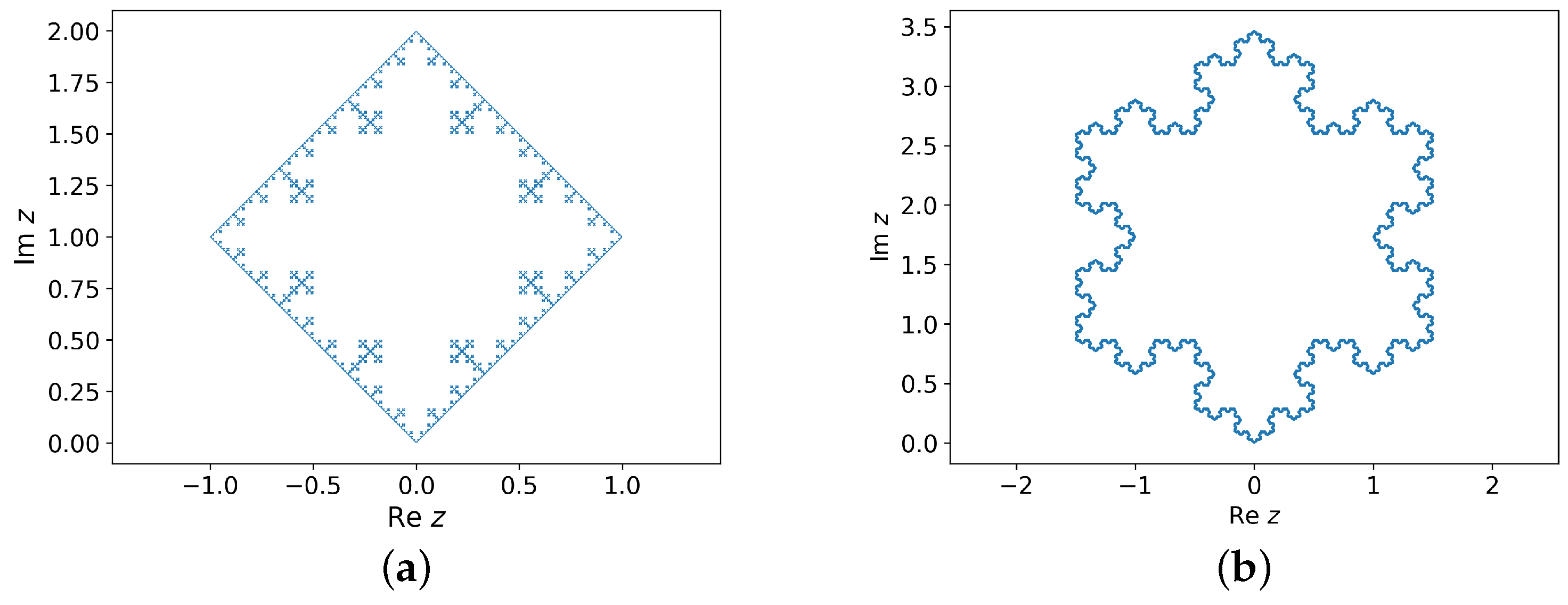
In this section, we give a few examples of numerical calculations for integrals over fractals. As test fractals, we choose the Koch snowflake and its analog based on scaled squares (see Figure 1a,b). We shall refer them to as fractals “a” and “b”. The corresponding fractal dimensions for the fractals “a” and “b” are $d(a)\approx 1.4650$ and $d(b)\approx 1.26196$.

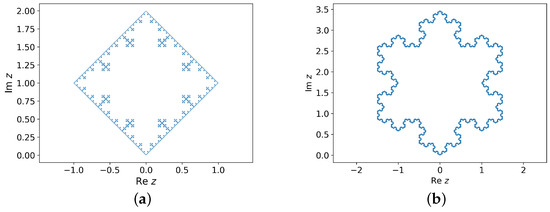
Figure 1. Fractals used in numerical examples: (a) an analogue of the Koch snowflake based on scaled squares; (b) the Koch snowflake.

As integrands, we use five functions. For examples of regular functions, we use

$$f_1(x,y)=x+2iy=\frac{3}{2}z-\frac{1}{2}\overline{z}$$

and

$$f_2(x,y)=e^{x+2iy}=e^{\frac{3}{2}z-\frac{1}{2}\overline{z}}.$$

As singular function integrands, we employ

$$f_3(z)=\frac{1}{z}$$

and

$$f_4(z,\overline{z})=\frac{{(\overline{z}+i)}^p}{z}p=1,3.$$

Finally, for an example of hypersingular integral, we use the following integrand

$$f_5(z,\overline{z})=\frac{a_0+a_{1}z+a_2{\overline{z}}^2}{z^2}.$$

We perform two versions of calculations for the corresponding contour integrals: the first is based on Formula (7) and its analog for the singular case (11), and the second corresponds to a direct calculation of the integral over the corresponding prefractals with mid-point or trapezoidal rules. The results of calculations for the integral ${\int }_{\mathsf{\Gamma }}{f}_{1,2}(z)dz$ for regular functions are given in Table 1. As the function $f_1$ is linear in both arguments, the midpoint rule gives an exact result for both approaches. The numerical results for a given order of the prefractal match exactly. The results for function $f_2$ obtained by direct calculation and by Formula (7) also agree well. This demonstrates the correctness of the integral over fractals definitions that we have been using.

Table 1. Convergence table for integrals ${\int }_{\mathsf{\Gamma }}{f}_i(z)dz$ of regular functions over fractal “a”. Here i stands for the imaginary unit.

Order	n	${\mathit{f}}_1$		${\mathit{f}}_2$
		Direct	(7)	Direct	(7)
0	4	−1i	−1i	0.889–0.571i	1.387–0.891i
1	20	−1.444i	−1.444i	1.616–1.037i	1.686–1.083i
2	100	−1.691i	−1.691i	1.885–1.210i	1.894–1.216i
3	500	−1.829i	−1.829i	2.016–1.295i	2.017–1.295i
4	2500	−1.905i	−1.905i	2.087–1.340i	2.087–1.340i
5	12,500	−1.947i	−1.947i	2.126–1.365i	2.126–1.365i
6	62,500	−1.971i	−1.971i	2.148–1.379i	2.147–1.379i
7	312,500	−1.984i	−1.984i	2.160–1.387i	2.160–1.387i
8	1,562,500	−1.991i	−1.991i	2.166–1.391i
9	7,812,500	−1.995i	-	2.170–1.393i	-
10	39,062,500	−1.997i	-	2.172–1.395i	-

The case of singular functions is less trivial. Even an elementary direct calculation of an integral over a contour meets some unexpected complications. In the example above we chose the step of the quadrature as the length of the corresponding prefractal side. This choice does not guarantee convergence to a correct result in some contour geometries.

Consider a sequence of contours composed of the prefractals for the fractal Figure 1 shifted so that the lowest side of each prefractal is centered at the singularity point $z=0+0i$ (Figure 2). The sides of the prefractal scale are $1/3^k$, where k is the order of the prefractal.

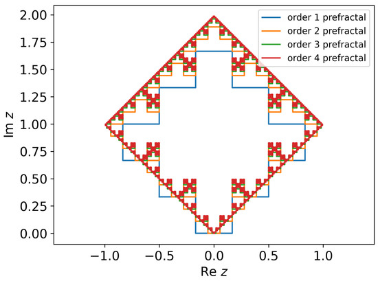
Figure 2. A sequence of prefractals used in singular integral example.

In order to calculate the singular integral over the contour, we employ the trapezoidal rule on each side of the prefractal. Even though the integration step goes to zero, any fixed order quadrature formula has a constant error contribution in the vicinity of the singular point. In order to compensate for this effect, we either have to use a sufficiently high order quadrature or further subdivide the sides of the prefractal. This effect has little to do with the fractal-like structure of the contour and can be also observed with piece-wise smooth contours of certain geometries. We attract the readers’ attention to this peculiarity only as a warning that the experience in numerical calculations of principal value integrals over real ranges does not always translate directly to their complex contour integral counterparts. The results of calculations are summarized in Table 2.

Table 2. Contour integral calculation results for function $f_3(z)=1/z$ over the contours shown in Figure 2. The first column indicates the order of the corresponding prefractal, and the second column contains the length of the corresponding prefractal side. The calculated real part of the integral does not exceed ${10}^{-10}$ and is not indicated. Take note that even though the prefractal side length approaches zero, there is a non-vanishing error in the evaluation of the singular integral. This error goes down, however, with more accurate quadrature formulas being used. Here i stands for the imaginary unit.

Order	Prefractal Side Length	Quadrature Rule
		Trapezoidal	Gaussian n = 2	Gaussian n = 4	Gaussian n = 6	(11)
0	1	3.20000i	3.19335i	3.14076i	3.14160i	$\pi i$
1	0.333	3.27940i	3.19616i	3.14078i	3.14160i	$\pi i$
2	0.111	3.27875i	3.19616i	3.14078i	3.14160i	$\pi i$
3	0.037	3.27853i	3.19616i	3.14078i	3.14160i	$\pi i$
4	0.0123	3.27850i	3.19616i	3.14078i	3.14160i	$\pi i$
5	0.00412	3.27849i	3.19616i	3.14078i	3.14160i	$\pi i$
6	0.00137	3.27849i	3.19616i	3.14078i	3.14160i	$\pi i$
7	0.000457	3.27849i	3.19616i	3.14078i	3.14160i	$\pi i$
8	0.000152	3.27849i	3.19616i	3.14078i	3.14160i	$\pi i$
9	5.08 $\times {10}^{-5}$	3.27849i	3.19616i	3.14078i	3.14160i	$\pi i$

As we have mentioned above, the singularity contribution $\pi if(t)$ when Formula (11) is employed strongly depends on the approximation of the fractal and can vary between 0 and $2\pi if(t)$. We have constructed the prefractal contours so that the singularity always strikes at the middle of one of the straight sides of the prefractal, which corresponds to the $\pi if(t)$, as if the fractal is approximated by a smooth contour. Here, we emphasize one more time that this choice is a result of a somewhat arbitrary convention that we make when performing singular integral calculations over a fractal. For instance, if we shift the prefractals in Figure 2 so that the singularity at $z=0$ hits the vertex of the prefractals rather than a midpoint of the side, the limiting fractal will be exactly the same, as the side length goes to zero, but the value of the integral would change from $\pi i$ to $\pi i/2$.

The results of calculations for $f_4(z,\overline{z})$ are summarized in Table 3. As the function is not analytical, unlike the previous example, the contribution of the double integral in Equation (11) is not trivial. Direct calculations are preformed using an eight-point Gauss–Legendre rule, which guarantees eight significant digits in our case. The results of direct calculations of the integral agree well with the calculations performed on the base of Formula (11). Again, the values that we report here are based on the same convention as in the previous example.

Table 3. Convergence table for integrals of a singular function $f_4(z,\overline{z})$ over the contours shown in Figure 2. The first column indicates the order of the corresponding prefractal, and the second column contains the length of the corresponding prefractal side.

Order	Side Length	$\mathit{p}=1$		$\mathit{p}=3$
		Direct	(11)	Direct	(11)
0	1	0.32242	0.85841	−3.57477	0.14159
1	0.333	0.81504	0.99404	−0.76477	−0.37710
2	0.111	0.97871	1.03837	0.07356	0.02639
3	0.037	1.10254	1.12243	0.32884	0.28685
4	0.0123	1.20064	1.20728	0.37339	0.35579
5	0.00412	1.27084	1.27306	0.35007	0.34372
6	0.00137	1.31705	1.31780	0.31504	0.31286
7	0.000457	1.34579	1.34604	0.28613	0.28539
8	0.000152	1.36300	1.36309	0.26623	0.26597
9	5.08 $\times {10}^{-5}$	1.37305	–	0.25366	–

Another enlightening example of the delicacy of singular integrals over fractals can be given by calculating the integrals of functions $f_3(z)$ and $f_4(z,\overline{z})$ over fractal “b”. Both approaches to the calculation of the integral

$${\int }_{{\gamma }_b}{f}_3(z)dz={\int }_{{\gamma }_b}\frac{dz}{z}=\frac{\pi }{3}i$$

give identical results provided the singularity contribution in Formula (11) is chosen correctly. But an infinitesimal—in the infinite prefractal order limits—shift of the contour to place the singularity at one of the nearest sides of the prefractals changes the result to $\pi i$. The numerical results for ${\int }_{{\gamma }_b}{f}_4(z,\overline{z})dz$ are given in Table 4.

Table 4. Convergence table for integrals of a singular function $f_4(z,\overline{z})$ over the fractal “b” prefractals (Koch snowflake). The first column indicates the order of the corresponding prefractal, and the second column shows the grid step for the evaluation of the double integral (11).

Order	Grid Step	$\mathit{p}=1$		$\mathit{p}=3$
		Direct	(11)	Direct	(11)
0	3	4.39420	10.9528	−2.63710	−2.17206
1	0.6	5.55701	7.18216	−2.87898	−4.17509
2	0.176	6.19947	7.06799	−3.18282	−4.95637
3	0.0566	6.53120	6.94534	−3.50067	−4.50142
4	0.0186	6.69404	6.82474	−3.69242	−4.01492
5	0.00619	6.77155	6.82638	−3.79339	−3.92664
6	0.00206	6.80771	6.83072	−3.84343	−3.89787
7	0.000686	6.82435	6.83403	−3.86739	−3.88961
8	0.000229	6.83194	6.83603	−3.87861	−3.88772

Finally, we give an example of a hypersingular integral calculation. We calculate the integral using Definition 12

$$\begin{array}{cc}\hfill {\int }_{{\gamma }_b}\frac{a_0+a_{1}z+a_2{\overline{z}}^2}{z^2}dz& =\frac{\pi i{a}_1}{3}+{\int }_{{\gamma }_b}\frac{a_2{\overline{z}}^{2}dz}{z^2}\hfill \end{array}$$

(16)

$$\begin{array}{cc}\hfill & =\frac{\pi i{a}_1}{3}+2i{\int \int }_{D_b^{+}}\frac{2a_2\overline{z}}{z^2}dxdy.\hfill \end{array}$$

(17)

The calculations have been performed with parameters $a_0=1$, $a_1=3$ and $a_2=1$. The results of calculations are given in Table 5. If no regularization is applied, the direct calculation of the contour integral at the left-hand side of Equation (16) is not feasible as the real part of the integral rapidly diverges. The imaginary part of the directly evaluated integral, however, is finite and evaluates to the values close to $\pi i{a}_1/3$ consistent with the results evaluated from (16) and (17).

Table 5. Convergence table for integrals of a hypersingular function (16) over the fractal “b” prefractals (Koch snowflake). The first column indicates the order of the corresponding prefractal, and the second column shows the grid step for the evaluation of the double integral in (17). Here i stands for the imaginary unit.

Order	Grid Step	(16)	(17)
0	3	−7.11720 + 3.14159i	−24.00000 + 3.14159i
1	0.6	−6.58614 + 3.14159i	−9.02423 + 3.14159i
2	0.176	−5.96004 + 3.14159i	−6.29219 + 3.14159i
3	0.0566	−5.59279 + 3.14159i	−5.51049 + 3.14159i
4	0.0186	−5.40095 + 3.14159i	−5.37218 + 3.14159i
5	0.00619	−5.30618 + 3.14159i	−5.27821 + 3.14159i
6	0.00206	−5.26090 + 3.14159i	−5.24412 + 3.14159i
7	0.000686	−5.23972 + 3.14159i	−5.23105 + 3.14159i
8	0.000229	−5.22995 + 3.14159i	−5.22578 + 3.14159i

6. Discussion and Conclusions

We have discussed definitions of regular, singular and hypersingular contour integrals over non-rectifiable curves and fractals. One of the main observation is in the difference between singular (hypersingular) integrals over piece-wise smooth curves and fractals. Let us emphasize this difference.

Consider an integral

$${\int }_{\mathsf{\Gamma }}\frac{f(\tau )}{\tau -t}d\tau ,t\in \mathsf{\Gamma },$$

where $\mathsf{\Gamma }$ is a closed bounded curve. Suppose that $\mathsf{\Gamma }$ is a smooth curve and $t\in \mathsf{\Gamma }$. The integral ${\int }_{\mathsf{\Gamma }}\frac{f(\tau )}{\tau -t}d\tau$ is a singular integral, and some regularization is required. The standard regularization method is

$${\int }_{\mathsf{\Gamma }}\frac{f(\tau )}{\tau -t}d\tau ={\int }_{\mathsf{\Gamma }}\frac{f(\tau )-f(t)}{\tau -t}d\tau +f(t){\int }_{\mathsf{\Gamma }}\frac{1}{\tau -t}d\tau .$$

It is known [1], that for a smooth closed curve

$${\int }_{\mathsf{\Gamma }}\frac{1}{\tau -t}d\tau =\pi i.$$

If $f(t)$ satisfies the Hölder condition, then ${\int }_{\gamma }\frac{f(\tau )-f(t)}{\tau -t}d\tau$ is a definite integral. To calculate it, we use standard quadrature formulas.

In some form or other, this scheme can be applied to the construction of quadrature formulas for the calculation of singular integrals.

Now, let $\mathsf{\Gamma }$ be a piece-wise smooth curve, and $t^{\ast }$ be a point where there is no tangent to the given curve. For $t=t^{\ast }$, the regularization of the integral ${\int }_{\mathsf{\Gamma }}\frac{f(\tau )}{\tau -t^{\ast }}d\tau$ is implemented by the formula [1]

$${\int }_{\mathsf{\Gamma }}\frac{f(\tau )}{\tau -t^{\ast }}d\tau ={\int }_{\mathsf{\Gamma }}\frac{f(\tau )-f(t^{\ast })}{\tau -t^{\ast }}d\tau +f(t^{\ast }){\int }_{\mathsf{\Gamma }}\frac{d\tau }{\tau -t^{\ast }}=$$

$$={\int }_{\mathsf{\Gamma }}\frac{f(\tau )-f(t^{\ast })}{\tau -t^{\ast }}d\tau +f(t^{\ast })i\alpha ,$$

where $\alpha$ is an angle between left and right tangents to the curve $\gamma$ at the point $t^{\ast }$.

For non-rectifiable curves, the construction described above is not applicable. There is, at least, a countable set of points where the curve $\mathsf{\Gamma }$ has no tangent lines. Moreover, left and right tangent lines may have different angles between them at different points. There are also curves with no tangent line at any point.

To calculate singular integral over a non-rectifiable curve or fractal, we implement the regularization similar to the regularization for a piece-wise smooth curve

$${\int }_{\mathsf{\Gamma }}\frac{f(\tau )}{\tau -t}d\tau ={\int }_{\mathsf{\Gamma }}\frac{f(\tau )-f(t)}{\tau -t}d\tau +f(t){\int }_{\mathsf{\Gamma }}\frac{d\tau }{\tau -t}.$$

The first integral is calculated by Stokes’s formula and the Whitney extension

$${\int }_{\mathsf{\Gamma }}\frac{f(\tau )-f(t)}{\tau -t}d\tau =\frac{2}{\pi }\int \int D^{+}\frac{\partial (\tilde{f}(z))}{\partial \tilde{z}}\frac{1}{z-t},$$

where $\tilde{f}(z)$ is the Whitney extension for f.

So,

$${\int }_{\mathsf{\Gamma }}\frac{f(\tau )}{\tau -t}d\tau =\frac{2}{\pi }\int \int D^{+}\frac{\partial (\tilde{f}(z))}{\partial \tilde{z}}\frac{1}{z-t}+f(t){\int }_{\mathsf{\Gamma }}\frac{d\tau }{\tau -t}.$$

(18)

The second integral $f(t){\int }_{\mathsf{\Gamma }}\frac{d\tau }{\tau -t}$ calculation depends on t. If t is a finite decimal or binary and, for a large enough N, it is included in the list of the vertices of the nth prefractals $(n\ge N)$, then we assume $f(t){\int }_{\mathsf{\Gamma }}\frac{d\tau }{\tau -t}=i{\alpha }_{N}f(t),$ here ${\alpha }_N$ is an angle between the left and the right tangent lines at the point t of the N-th order prefractal. If the condition is not fulfilled, any value between 0 and $2\pi$ can be ascribed to the integral ${\int }_{\mathsf{\Gamma }}\frac{d\tau }{\tau -t}$.

Singular and hypersingular integrals are particular cases of generalized functions. In the theory of generalized functions [38,41], there is a known statement that all the regularizations differ by a constant. Within this approach, it is legitimate to define—according to Mironova [37]—a singular integral as

$$\frac{1}{\pi i}{\int }_{\mathsf{\Gamma }}\frac{f(\tau )}{\tau -t}d\tau =f(t)-\frac{1}{\pi i}{\int }_{D^{+}}\frac{\partial (\tilde{f}(z))}{\partial \overline{z}}\frac{1}{z-t}dzd\overline{z},$$

where $\tilde{f}(z)$ is the Whitney extension for f.

In this work, we define a singular integral by using Formula (18). This approach is substantiated by the representation of the singularity point t. If t is presented as an infinite fraction, then, when solving a particular problem, its value has to be approximated by a finite decimal fraction. Therefore, by choosing an approximate representation of t and the prefractal sequence, which approximates the fractal curve, the researcher ascribes the value to the singular integral $\int \frac{d\tau }{\tau -t}$ according to the problem being solved. (It seems that further generalizations of this construction are also possible. For instance, singular and hypersingular integrals over fractals could be treated as stochastic objects with distributions depending on the fractal curve. This approach, however, is subject to future research).

The stability of quadrature and cubature formulas for one- and multi-dimensional singular integrals has been studied in the monograph [11]. Upper bounds of the errors for a number of cubature formulas have been obtained assuming an $\epsilon$-perturbation of the integrands. Besides the upper bounds, for some cubatures, the expected values for the errors have also been given. These results can be easily transferred to the cubatures discussed in the article.

Similar arguments are applicable to quadrature formulas for hypersingular integrals.

In this paper, we have constructed quadrature and cubature formulas for the calculation of Riemann, singular and hypersingular integrals over non-rectifiable curves and fractals. Some quadrature and cubature formulas have been constructed based on various definitions of integrals over non-rectifiable curves and fractals. We obtained error estimates on classes of functions having derivatives of the first order satisfied the Hölder condition with $\alpha ,0<\alpha \le 1$.

The obtained results show that having derivatives greater than the first order does not affect the accuracy of cubature formulas with rectangular grids. To increase the accuracy of cubature formulas, it is necessary to construct cubature formulas with several grids, which account for the boundary layer. A similar problem arises when we construct cubature formulas to calculate integrals over non-rectifiable curves and fractals based on the Whitney extension. This is caused by the feature of Whitney’s extension: the extension $u(z)$ of function $f(z)$ defined on the boundary $\mathsf{\Gamma }$ of region D has derivatives of the first order in $D\backslash \mathsf{\Gamma }$ and $|\mathrm{grad}u(z)|\le K{(\mathrm{dist}(z,\mathsf{\Gamma }))}^{\alpha -1}$, $K=\mathrm{const}$.

The authors intend to construct cubature formulas with variable grids accounting for the boundary layer in future works.

References

- Gakhov, F.D. Boundary Value Problems; Dover Publication: Mineola, NY, USA, 1990. [Google Scholar]
- Boykov, I.V.; Boykova, A.I. Analytical methods for solution of hypersingular integral equations. Univ. Proc. Volga Reg. Phys. Math. Sci. 2017, 2, 63–78. [Google Scholar]
- Boykov, I.V.; Boykova, A.I. Analytical methods for solution of hypersingular and polyhypersingular integral equations. arXiv 2019, arXiv:1901.04880v1. [Google Scholar]
- Lifanov, I.K. Singular Integral Equations and Discrete Vortices; VSP: Utrecht, The Netherlands, 1996. [Google Scholar]
- Boykov, I.V. Approximate Methods of Solution of Singular Integral Equations; Penza State University Publishing House: Penza, Russia, 2004. [Google Scholar]
- Golberg, M.A. The convergence of several algorithms for solving integral equations with finite-part integrals, I. J. Integral Equ. 1983, 5, 329–340. [Google Scholar]
- Golberg, M.A. The convergence of several algorithms for solving integral equations with finite-part integrals, II. J. Integral Equ. 1985, 9, 267–275. [Google Scholar]
- Lifanov, I.K.; Poltavskii, L.N.; Vainikko, G.M. Hypersingular Integral Equations and Their Applications; CRC Press Company: Boca Raton, FL, USA, 2004. [Google Scholar]
- Boykov, I.; Roudnev, V.; Boykova, A. Approximate methods for solving linear and nonlinear hypersingular integral equations. Axioms 2020, 9, 74. [Google Scholar] [CrossRef]
- Boykov, I.V. Approximate methods for solving hypersingular integral equations. In Topics in Integral and Integro-Difference Equations. Theory and Applications; Singh, H., Dutta, H., Cavalcanti, M.M., Eds.; Springer: Dordrecht, The Netherlands, 2021; pp. 63–102. [Google Scholar]
- Boykov, I.V. Approximate Methods for Calculating Singular and Hypersingular Integrals. Part One. Singular Integrals; Penza State University Publishing House: Penza, Russia, 2005. [Google Scholar]
- Boykov, I.V. Approximate Methods for Calculating Singular and Hypersingular Integrals. Part Two. Hypersingular Integrals; Penza State University Publishing House: Penza, Russia, 2009. [Google Scholar]
- Boykov, I.V.; Ventsel, E.S.; Boykova, A.I. Accuracy optimal methods for evaluating hypersingular integrals. Appl. Numer. Math. 2009, 59, 1366–1385. [Google Scholar] [CrossRef]
- Boykov, I.V.; Boykova, A.I.; Aikashev, P.V. Projection methods for solving hypersingular integral equations on fractals. Univ. Proc. Volga Reg. Phys. Math. Sci. Math. 2016, 1, 71–86. [Google Scholar]
- Boykov, I.V.; Boykova, A.I.; Potapov, A.A.; Rassadin, A.E. Approximate Methods for Solving Hypersingular Integral Equations on Fractals. In 14th Chaotic Modeling and Simulation International Conference. CHAOS, Greece, 2021; Skiadas, C.H., Dimotikalis, Y., Eds.; Springer Proceedings in Complexity; Springer: Cham, Switzerland, 2022. [Google Scholar]
- Kats, B.A.; Mironova, S.R.; Pogodina, A.Y. Singular Integral Equations on Non-Smooth Curves in Hölder-Frechet Space. Russ. Math. Iz. VUZ 2018, 10, 26–29. [Google Scholar] [CrossRef]
- Jaggard, D.L.; Jaggard, A.D. Polyadic Cantor Superlattices with Variable Lacunarity. Opt. Lett. 1997, 22, 145–147. [Google Scholar] [CrossRef]
- Puente, C.; Romeu, J.; Pous, R.; Cardama, A. On the Behavior of the Sierpinski Multiband. Fractal Antenna IEEE Trans. Antennas Propag. 1998, 46, 517–524. [Google Scholar] [CrossRef]
- Potapov, A.A. Fractals in Radiophysics and Radar: The Topology of the Sample; Universitetskaya Kniga: Moscow, Russia, 2005. [Google Scholar]
- Werner, D.H.; Gangul, S. An Overview of Fractal Antenna. Eng. Res. IEEE Antennas Propag. Mag. 2003, 45, 38–57. [Google Scholar] [CrossRef]
- Turcotte, D. Fractals and Chaos in Geology and Geophysics; Cambridge University Press: Cambridge, UK, 1992. [Google Scholar]
- Babayants, P.S.; Blokh, Y.I.; Trusov, A.A. Fundamentals of modeling potential fields of fractal geological objects. In Questions of Theory and Practice of Geological Interpretation of Gravitational, Magnetic and Electric Fields. Proceedings of the 32nd Session of the International Seminar Named after D.G. Uspensky; Mining Institute of the Ural Branch of the Russian Academy of Sciences: Perm, Russia, 2005; pp. 12–14. [Google Scholar]
- Chikin, L.A. Special cases of the Riemann boundary value problems and singular integral equations. Sci. Notes Kazan State Univ. 1953, 113, 53–105. [Google Scholar]
- Stein, I. Singular Integrals and Differential Properties of Functions; Mir: Moscow, Russia, 1973. [Google Scholar]
- Kondurar, V. Sur l’integrale de Stieltjes. Rec. Math. Moscou 1937, 2, 361–366. [Google Scholar]
- Kats, B.A. The Stieltjes integral over a fractal contour and some of its applications. Russ. Math. 2000, 44, 19–29. [Google Scholar]
- Wiener, N. The quadratic variation of a function and its Fourier coefficients. J. Math. Phys. 1924, 3, 72–94. [Google Scholar] [CrossRef]
- Young, L.C. An inequality of the Hölder type, connected with Stieltjes integration. Acta Math. Upps. 1936, 36, 251–282. [Google Scholar] [CrossRef]
- Young, L.C. General inequalities for Stieltjes integrals and the convergence of Fourier series. Math. Ann. 1938, 115, 581–612. [Google Scholar] [CrossRef]
- Kats, B.A. Jump problem and integral over non-rectifiable curve. Sov. Math. 1987, 31, 65–75. [Google Scholar]
- Harrison, J.; Norton, A. The Gauss–Green theorem for fractal boundaries. Duke Math. J. 1992, 67, 575–586. [Google Scholar] [CrossRef]
- Harrison, J. Stokes theorem for nonsmooth chains. Bull. Am. Mat. Soc. 1993, 29, 235–242. [Google Scholar] [CrossRef]
- Kats, B.A. Integration over Non-Rectifiable Curve; Issues of Mathematics, Continuum Mechanics and Application of Mathematical Methods in Construction: Collection of Scientific Papers; MGSU, MSUCE: Moscow, Russia, 1992; pp. 63–69. [Google Scholar]
- Kats, B.A. Integration over a plane fractal curve, a jump problem and generalized measure. Russ. Math. 1998, 42, 51–63. [Google Scholar]
- Kats, B.A. Integration over a fractal curve and the jump problem. Math. Notes 1998, 64, 476–482. [Google Scholar] [CrossRef]
- Vekua, I.N. Generalized Analytic Functions, 2nd ed.; Olejnik, O.A., Shabat, B.V., Eds.; Nauka: Moscow, Russia, 1988. [Google Scholar]
- Mironova, S.R. Singular integral equations on countable set of closed non-rectifiable and fractal curves. Russ. Math. 1998, 42, 41–47. [Google Scholar]
- Gel’fand, I.M.; Shilov, G.E. Generalized Functions. Volume 1: Properties and Operations; AMS Chelsea Publishing, American Mathematical Society: Providence, RI, USA, 2016. [Google Scholar]
- Potapov, A.A.; Gulyaev, Y.V.; Nikitov, S.A.; Pakhomov, A.A.; German, V.A. The Modern Methods of Image Processing; Potapov, A.A., Ed.; FIZMATLIT: Moscow, Russia, 2008. [Google Scholar]
- Natanson, I.P. Constructive Function Theory. Vol. I. Uniform Approximation; Frederick Undar Publishing Co.: New York, NY, USA, 1965. [Google Scholar]
- Schwartz, L. Théorie des Distributions; Hermann: Paris, France, 1966. [Google Scholar]
Disclaimer/Publisher’s Note: The statements, opinions and data contained in all publications are solely those of the individual author(s) and contributor(s) and not of MDPI and/or the editor(s). MDPI and/or the editor(s) disclaim responsibility for any injury to people or property resulting from any ideas, methods, instructions or products referred to in the content. |
© 2023 by the authors. Licensee MDPI, Basel, Switzerland. This article is an open access article distributed under the terms and conditions of the Creative Commons Attribution (CC BY) license (https://creativecommons.org/licenses/by/4.0/).