Optimal Shipping Route under the Designation of the Mediterranean Sulfur Emission Control Area: Mathematical Models and Applications

Abstract

In order to tackle sulfur oxides (${\mathrm{SO}}_{\mathrm{x}}$) emissions from maritime activities, both local governmental bodies and the International Maritime Organization (IMO) have implemented a range of regulations with the establishment of sulfur emission control areas (SECAs) being one crucial measure. Recently, the IMO made the significant decision to designate the Mediterranean as an SECA, aiming to promote environmental conservation as well as sustainable development in the maritime industry and mitigate the adverse health effects caused by air pollutants emitted from ships in Mediterranean regions. While this policy signifies significant progress in the reduction of sulfur emissions, it simultaneously presents intricate challenges for maritime enterprises. Notably, under the Mediterranean SECA designation, shipping companies may opt to bypass this region and choose routes through the Cape of Good Hope as a means of minimizing the overall costs, resulting in a potential increase in global carbon emissions. To support shipping companies in formulating optimal strategies within the framework of this new policy, the research introduces advanced techniques to make the optimal decisions concerning route selection, sailing speeds, and the appropriate number of ships for both SECAs and non-SECAs. Furthermore, we elucidate how these optimal decisions can be dynamically adapted in response to the dynamic fluctuations in fuel prices and the weekly operational expenditures incurred by maritime fleets. In the experimental results, taking into account factors like route distance and fuel costs, shipping companies select routes through the Mediterranean region in both eastward and westward directions. The total cost amounts to $6,558,766.78, utilizing eight vessels. Regarding ship speeds, vessels sail at reduced speeds in SECAs compared to non-SECAs. Furthermore, longer voyage distances require deploying a greater number of ships to maintain a weekly service frequency. This research exhibits robust timeliness and practicality, which is in line with practice. It not only timely supplements and enhances the extant body of knowledge concerning SECAs but also serves as a valuable point of reference and emulation for shipping companies seeking to optimize their operations within the framework of the new policy landscape. Furthermore, it offers pertinent insights for the IMO in formulating policies related to SECAs.

1. Introduction

Maritime transportation is the backbone of the global trade and manufacturing supply chain [1]. According to the report of the United Nations Conference on Trade and Development, more than 80% of world merchandise trade by volume is carried by sea in 2021 [1]. However, tremendous shipping volume also poses great burdens on the environment and sustainable development, as it produces huge carbon emissions and plenty of toxic pollutants, such as sulfur oxides (${\mathrm{SO}}_{\mathrm{x}}$) emissions, that directly threaten human health. In particular, maritime transportation accounts for 12% of global anthropogenic ${\mathrm{SO}}_{\mathrm{x}}$ emissions [2]. In addition, the ships burn bunker fuel, which has a much higher sulfur content than that of other transportation modes. These ${\mathrm{SO}}_{\mathrm{x}}$ emissions have caused serious air pollution around the coastal area, which has harmful effects on human health as well as ecosystems.

To control ${\mathrm{SO}}_{\mathrm{x}}$ emissions from shipping, the local government and IMO have implemented a series of regulations around the world. For instance, the Hong Kong Environmental Protection Department has prohibited the use of high-sulfur fuel when ships are at berth [3]. The Maritime and Port Authority of Singapore has reduced the port fees for vessels that use low-sulfur fuel [4]. The IMO has imposed a smaller global sulfur cap of 0.5% from the previous 3.5%, which has been effective since 1 January 2020. Another effective measure enforced by the IMO to reduce shipping pollution is setting down several sulfur emission control areas (SECAs) across the globe, where the fuel used by vessels within the SECAs should have a lower sulfur cap, i.e., 0.1%, than that in most ocean areas, i.e., 0.5%. By November 2022, the IMO has established SECAs including the Baltic Sea, the North Sea, the North American region and the United States Caribbean Sea area.

Recently, to reduce the ${\mathrm{SO}}_{\mathrm{x}}$ emissions from shipping and improve the air quality in port cities, the IMO has planned to designate the Mediterranean Sea as a new SECA, which will become effective from from 1 January 2025 [5]. According to the feasibility study conducted by [6], the effects of the implementation of an SECA in the Mediterranean Sea are generally positive. To be specific, the approved amendment sets a stringent limit of 0.10% mass by mass (m/m) for sulfur content in fuel oil utilized onboard ships within specific areas. Outside these designated zones, the prevailing limit remains at 0.50% m/m. Additionally, the study demonstrates that implementing the new SECA will reduce the ${\mathrm{SO}}_{\mathrm{x}}$ emissions in Mediterranean areas by 95% compared to 2015. Furthermore, according to the report published by the International Institute for Applied Systems Analysis (IIASA) [7], there will be respective reductions of 80% and 20% in sulfur dioxide and nitrogen oxide emissions accompanied by a simultaneous decrease of 62% in particulate matter (PM) emissions. These emission reductions surpass the standards mandated by MARPOL VI regulations by 11 percentage points. Moreover, the cost–benefit analysis validates the efficiency of establishing an SECA to limit the harmful health effects of exposure to shipping air pollutant emissions in Mediterranean areas. Naturschutzbund Deutschland (NABU) demonstrates that the decision will considerably enhance air quality for nearly 150 million individuals residing in the Mediterranean region [8].

Nevertheless, despite the overall advantages revealed by the feasibility study, the net impact of the implementation of an SECA in the Mediterranean Sea on air pollution is assessed without considering its influence on future shipping course choice. It should be pointed out that there are generally two methods to cope with the sulfur cap limitation. One method is to switch to cleaner energies, such as low-sulfur fuel oil and natural gas [9,10]. Currently, there is widespread attention directed toward the utilization of clean fuels. Ultra-low-sulfur diesel fuel with a sulfur content lower than 0.0015% has been implemented for marine diesel engines particularly in ships operating within SECAs [11]. Moreover, there is an ongoing exploration into the comprehensive overview of efficient and clean energy utilization as an intelligent strategy for reducing CO${}_2$ emissions along the port-to-ship pathway [12]. However, clean energy sources come at a significantly higher cost compared to conventional bunker fuels. Consequently, the judicious management of ship fuel consumption and navigation time has emerged as a pressing necessity in achieving the sustainable development of the maritime industry [13]. Another method is installing scrubbers for sulfur exhaust disposal, which also raises the shipping price. The open loop scrubbers, which utilize seawater to scrub the exhaust gases, have even been prohibited by a growing number of ports because discharging exhaust water could potentially pollute the marine environment [14]. For all these reasons, the implementation of a Mediterranean SECA may force ships to take alternative routes instead of traveling through the Mediterranean Sea.

A highly possible consequence is the change of course for ships between Asia and Europe. Currently, most of the ships from Asia to Europe prefer to sail through the Red Sea, the Suez Canal and across the Mediterranean Sea, which is about 3000 nautical miles shorter than sailing around the Cape of Good Hope. However, if the Mediterranean Sea is designated as an SECA, the sailing route through the Suez Canal is no longer economical and practical for ships sailing between Europe and Asia, and most of these ships may choose the route around the Cape of Good Hope as a substitute. Therefore, the designation of the Mediterranean SECA may result in longer sailing distances, which will give rise to carbon emissions. The exacerbation of greenhouse effects goes against our original intention of promoting environmentally friendly and sustainable shipping. In fact, the carbon emissions from shipping activities are not negligible. According to the fourth IMO greenhouse gas study in 2020, 2.89% of the world’s carbon emissions come from international shipping [2]. What is worse, the carbon emissions from international shipping are expected to rise by 50% to 250% by 2050, mostly as a result of the expansion of global marine trade [15]. At the same time, countries and international organizations have been implementing various policy measures to control carbon emissions, aligning with the United Nations’ Sustainable Development Goals (SDGs). These goals aim to comprehensively address social, economic, and environmental dimensions of development from 2015 to 2030, promoting a shift toward sustainable pathways. In 2015, the Paris Agreement saw 196 parties committing to transform their development trajectories toward sustainability and limit global warming to well below 2 °C, ideally 1.5 °C, above pre-industrial levels. Achieving these targets requires a 45% reduction in global carbon dioxide emissions by 2030 compared to 2010 levels, ultimately reaching net-zero emissions by 2050. To demonstrate their commitment, countries submit nationally determined contributions (NDCs) outlining their voluntary efforts to reduce emissions and adapt to climate change impacts. Each party is encouraged to prepare, communicate, and update successive NDCs. By May 2021, 192 parties had submitted their initial NDCs to the Framework Convention on Climate Change secretariat. Additionally, as of December 2020, 48 parties had submitted new or updated NDCs, representing 75 parties and accounting for 30% of global greenhouse gas emissions in 2017. Notably, 39 of these NDCs incorporated adaptation information [16]. Thus, the possible rise of carbon emissions caused by the establishment of SECA in the Mediterranean Sea should be considered seriously.

Within this study, we put forward mathematical models to facilitate optimal decision making aimed at minimizing costs for shipping companies while adhering to the recently implemented IMO policy on the establishment of SECAs. Our study addresses the following research inquiries:

• Following the designation of the Mediterranean as an SECA, will shipping companies opt to bypass this region and choose routes via the Cape of Good Hope to reduce overall costs?
• What are the optimal sailing speeds and travel times, both within SECAs and non-SECAs, along each route that minimize total costs for shipping companies under the new IMO SECA policy?
• Considering the Mediterranean’s SECA status, what is the optimal number of equipped ships for the shipping route that leads to the lowest total costs?

To tackle these three research questions, we initially propose a mixed-integer nonlinear programming (MINLP) model that presents challenges due to its complexity and intricate problem solving. Leveraging the inherent structure of the model, we strategically partition it into four sub-models based on route selection. Subsequently, we convert the nonlinear optimization model into mixed-integer linear programming (MILP) models by employing piecewise-linear functions to achieve an approximation of the nonlinear function. These MILP models can be efficiently resolved using readily available optimization solvers. Lastly, we conduct experiments and perform sensitivity analyses to assess the models’ performance under varying parameter conditions. These experiments allow us to gauge the models’ effectiveness and assess its robustness in the face of parameter fluctuations.

1.1. Literature Review

1.1.1. The Establishment of SECAs

Emissions from maritime vessels operating in coastal areas and ports have a significant impact on the quality of the surrounding regional and local air [17]. In response, the IMO has implemented regulations with the aim of reducing the release of ${\mathrm{SO}}_{\mathrm{x}}$ into the atmosphere. However, it is recognized that the global impact of these regulations on air quality improvement is relatively modest and happens over an extended period of time. Therefore, additional legislation with more stringent measures has been gradually introduced in specific areas known as SECAs. The establishment of SECAs holds paramount significance for the shipping industry and the attainment of global sustainable development objectives. Not only does it play a crucial role in mitigating the adverse environmental impacts posed by sulfur emissions from maritime vessels, but also it fosters a transition toward cleaner and greener shipping practices. By reducing sulfur emissions, SECAs contribute to the global reduction of greenhouse gas emissions, aligning with the targets set forth in international agreements such as the Paris Agreement and Sustainable Development Goals.

Throughout the 1980s, the IMO implemented a series of measures aimed at controlling noxious gas emissions from shipping and mitigating air pollution. The MARPOL (International Convention for the Prevention of Pollution from Ships) has progressively adopted provisions for the establishment of ECAs [18]. And since 2006, the IMO’s International Convention for the Prevention of Pollution from Ships (MARPOL) Annex VI, titled “Preventing Air Pollution from Ships” [19], has implemented a general limit on sulfur oxide emissions from ships. By far, Annex VI of MARPOL has undergone successive revisions, leading to a gradual reduction in the permissible sulfur content from 4.5% to 0.5% [20]. The implementation of IMO 2020 further tightens the sulfur limit for fuel oil, setting it at 0.50% m/m outside SECAs and 0.1% within SECAs, which is effective from 1 January 2020 [21]. Notably, in 2015, the North American and Northern European ECAs took the initiative to establish SECAs with a stringent upper limit of 0.1% m/m for sulfur content [18]. These initiatives were crucial in curbing emissions and promoting environmental sustainability within these designated areas. This global limitation on sulfur content in fuels represents a substantial shift in the industry and necessitates that each shipping company carefully weigh their compliance options to simultaneously reduce emissions and sustain profitability within the framework of the policy conditions.

In the regional perspective, MARPOL has delineated four distinct regions known as ECAs, including the Baltic Sea, the North Sea, the English Channel, and coastal waters surrounding the United States, Canada, and the US Caribbean Sea. It is noteworthy that the North American and US Caribbean ECAs also regulate nitrogen oxide (${\mathrm{NO}}_{\mathrm{x}}$) emissions, further emphasizing the comprehensive approach toward environmental preservation [22]. Furthermore, the European Union (EU) has adopted legislation that combines the regulations set forth by the IMO into EU law, which are exemplified by the latest iteration known as Directive 2012/33/EU, commonly referred to as the sulfur directive. These measures underline the proactive steps being taken to safeguard our environment and ensure sustainable maritime practices [23].

1.1.2. The Optimal Decisions with the SECAs

The establishment of SECAs undoubtedly exerts a significant influence on the optimal decision making of shipping companies. Specifically, in terms of fuel selection, ships have to choose more expensive low-sulfur fuels when navigating within SECAs. Typically, fuel consumption exhibits a cubic relationship with ship sailing speed [24]. Studies conducted by [23,25] focused on the optimization problem of sailing speed within SECAs. They discovered that ships tend to operate at lower speeds inside SECAs and higher speeds outside SECAs. Consequently, higher sailing speeds outside SECAs result in increased emissions in those areas. Dulebenets [26] investigated the ship scheduling problem with sailing speed optimization, considering the impact of ECAs (including SECAs) and transit time constraints. Sheng et al. [27] solved the optimization of ship steaming speed and fleet size for an industrial shipping service under SECAs regulations. Their findings indicated that these regulations effectively reduce regional sulfur emissions. Fagerholt et al. [23] investigated the optimization problem of sailing patterns (route and speed) within ECAs. Numerical results for various realistic ship routes showed that ships would sail longer distances outside SECAs, leading to increased fuel consumption and emissions for certain routes. In order to delve further into the optimization problem of sailing patterns within ECAs, Ref. [28] proposed a bi-objective mixed-integer linear programming model to minimize both fuel costs as well as sulfur emissions. The results demonstrated the efficacy of this model in saving fuel costs and reducing sulfur emissions in compliance with SECAs regulations. To adhere to the regulations within SECAs, the maritime industry and research community have devised diverse strategies and technologies aimed at reducing sulfur emissions [29,30]. These strategies encompass a spectrum of initiatives, including the adoption of shore power, fuel conversion, the installation of exhaust gas scrubbers, and the incorporation of liquefied natural gas (LNG) propulsion for vessels, among others. Currently, fuel conversion has emerged as a pivotal choice in mitigating sulfur emissions, particularly for aging vessels, as noted by [31]. Projections put forth by [32] indicate that LNG and biofuels are poised to constitute 50% of the shipping sector’s energy demand by 2050, thereby forecasting significant reductions in ship exhaust emissions. Furthermore, Jiang et al. [33] conducted a comprehensive analysis of the cost-effectiveness and environmental benefits associated with MGO and Heavy Fuel Oil (HFO) coupled with scrubber technology. Their findings underscored the potential to achieve up to a 98% reduction in sulfur emissions for HFO with scrubbers and a 90% reduction for MGO. Similarly, Panasiuk and Turkina [34] undertook a comparative study between low-sulfur fuel and high-sulfur fuel with scrubber systems, demonstrating that scrubbers have the capability to curtail sulfur emissions by an impressive 90–99%. In another comparative analysis by [35], the utilization of low-sulfur marine diesel was juxtaposed with the installation of scrubber systems, revealing that when scrubbers are employed, both fuel consumption and ship emissions tend to experience an uptick.

In a broader context, numerous countries and international organizations have already introduced a series of measures to address carbon and sulfur emissions issues with the establishment of SECAs being a significant component among them. Designating the Mediterranean Sea as an SECA is a newly enacted policy. However, the Mediterranean’s unique geographical location renders it a pivotal strategic maritime hub, which means the implementation of this new policy undoubtedly bears implications for shipping companies’ decisions pertaining to route selection and fuel choices, thereby impacting overall societal carbon and sulfur emissions. For instance, in the context of the Eurasian shipping routes, certain shipping companies may opt for longer routes via the Cape of Good Hope over Mediterranean routes due to stringent sulfur emission regulations, consequently resulting in elevated levels of both carbon and sulfur emissions. Hence, this study serves as a timely and comprehensive supplement to existing research on SECAs, possessing a strong timeliness and applicability. It offers valuable insights for shipping companies in making optimal decisions and serves as a reference for the IMO and related organizations in formulating subsequent policies regarding SECAs.

1.2. Research Contributions

1.

Theoretical contributions. This study has undertaken a timely and meticulous supplement of existing research concerning SECAs, which has been driven by the recent introduction of a new policy by the IMO designating the Mediterranean as an SECA. This research is up to date and takes into full account the unique geographical attributes of the Mediterranean. It conducts a thorough analysis of the potential implementation effects of this policy with particular consideration given to the possible implications for increased carbon and sulfur emissions. Furthermore, it offers valuable insights for the subsequent development of IMO policies related to SECAs, serving as a pivotal point of reference and a source of inspiration. The proposed approach entails a nonlinear optimization model to derive the optimal decisions of shipping companies. Leveraging the distinctive structure of the optimization problem under the new IMO policy, we decompose the original model into four sub-models. Additionally, we transform the nonlinear models into four solvable MILP models by approximating the nonlinear function using piecewise-linear functions. Through rigorous experiment and sensitivity analyses, we obtain specific solutions and assess the impact of different parameters.

2.

Practical contributions. This study possesses a high degree of applicability, providing optimal strategies that enable shipping companies to reduce costs and align with the newly established IMO policy designating the Mediterranean as an SECA. The insights gained carry significant practical implications for fostering the sustainable advancement of the shipping industry while ensuring strict compliance with environmental regulations. The proposed mathematical model stands as a decision-making instrument for shipping companies grappling with the complexities and possibilities arising from the implementation of the new IMO policy.

The rest of the paper is organized as follows. Section 2 describes the research problem in detail and develops the mathematical model. Section 3 proposes solution methods for addressing the initial proposed model. Section 4 includes the experiments and sensitivity analysis. Finally, conclusions are drawn in Section 5.

2. Problem Description and Model Development

As discussed in Section 1, while the establishment of an SECA in the Mediterranean Sea is effective in reducing ${\mathrm{SO}}_{\mathrm{x}}$ emissions, it may cause more carbon emissions. This is because vessels might opt to alter their routes, choosing to circumnavigate the Cape of Good Hope instead of traversing the Red Sea, transiting the Suez Canal, and crossing the Mediterranean Sea.

We consider a vessel company that provides shipping service between Asia and Europe in two sailing directions: eastward direction and westward direction. For each sailing direction, vessels have the option to traverse the new SECA area, which is the Mediterranean Sea. Alternatively, they can choose to take the longer route around the Cape of Good Hope, thereby avoiding restrictions on ${\mathrm{SO}}_{\mathrm{x}}$ in the SECA area. We use binary decision variables $z_1$ and $z_2$ to denote whether to pass through the new SECA area or not. Specifically, $z_1$ equals 1 if the eastward direction that includes the new SECA area is selected and 0 otherwise; $z_2$ equals 1 if the westward sailing direction that includes the new SECA area is selected and 0 otherwise.

The total sailing lengths of the routes without the SECA area on the eastward direction and westward direction are denoted by $l_1^{\mathrm{G}}$ and $l_2^{\mathrm{G}}$, respectively. That is, the vessel chooses to circumnavigate the Cape of Good Hope. The vessel can also select the route with the SECA area (i.e., the Mediterranean Sea). The total sailing length of the route containing the SECA area is the sum of the sailing length of the SECA area and the sailing length of the non-SECA area in this route. We use $l_1^{\mathrm{M}\text{-}\mathrm{ECA}}$ and $l_2^{\mathrm{M}\text{-}\mathrm{ECA}}$ to denote the sailing lengths of the routes within the SECA area on the eastward direction and westward direction, respectively. Similarly, $l_1^{\mathrm{M}\text{-}\mathrm{NECA}}$ and $l_2^{\mathrm{M}\text{-}\mathrm{NECA}}$ denote the sailing lengths of the routes out of the SECA area on the eastward direction and westward direction, respectively.

When sailing across SECA areas, vessels have to use marine gas oil (MGO), which has a lower sulfur cap (0.1%) than that in most low-sulfur fuel oil (LSFO) (0.5%). However, the price of MGO is much higher than LSFO. We use $\gamma$ and $\beta$ to denote the price per tonne of MGO and LSFO, respectively.

The decision-making process of the vessel company encompasses several aspects, including selecting the route for vessels, determining the optimal sailing speed, and specifying the number of deployed vessels. Since the vessel company is self-interested, its goal is to minimize the total operating costs, including the fuel cost and the fixed cost of vessels. We use x to denote the number of deployed vessels. The total number of available vessels in the vessel company is X. The fixed cost of one vessel is c per day. We define the following decision variables regarding the sailing speeds for model formulation:

• $v_1^{\mathrm{G}}$ is the sailing speed on the route without SECA areas in the eastward direction.
• $v_2^{\mathrm{G}}$ is the sailing speed on the route without SECA areas in the westward direction.
• $v_1^{\mathrm{M}\text{-}\mathrm{NECA}}$ represents the sailing speed when passing through non-SECA areas in the route including SECA areas in the eastward direction.
• $v_1^{\mathrm{M}\text{-}\mathrm{ECA}}$ represents the sailing speed when passing through SECA areas in the route including SECA areas in the eastward direction.
• $v_2^{\mathrm{M}\text{-}\mathrm{NECA}}$ represents the sailing speed when passing through non-SECA areas in the route including SECA areas in the westward direction.
• $v_2^{\mathrm{M}\text{-}\mathrm{ECA}}$ represents the sailing speed when passing through SECA areas in the route including SECA areas in the westward direction.

Referring to [36], the power-of-k relation is adopted to describe the relationship between sailing speed and fuel consumption, and the most common assumption is the cubic relationship, i.e., k = 3. To achieve cost minimization, we formulate the following model.

[M1]

$$\begin{array}{c}\hfill mincx+a\gamma \left(\frac{l_1^{\mathrm{M}\text{-}\mathrm{ECA}}}{v_1^{\mathrm{M}\text{-}\mathrm{ECA}}}\times {\left(v_1^{\mathrm{M}\text{-}\mathrm{ECA}}\right)}^3+\frac{l_2^{\mathrm{M}\text{-}\mathrm{ECA}}}{v_2^{\mathrm{M}\text{-}\mathrm{ECA}}}\times {\left(v_2^{\mathrm{M}\text{-}\mathrm{ECA}}\right)}^3\right)+\\ \hfill a\beta \left(\frac{l_1^{\mathrm{M}\text{-}\mathrm{NECA}}}{v_1^{\mathrm{M}\text{-}\mathrm{NECA}}}\times {\left(v_1^{\mathrm{M}\text{-}\mathrm{NECA}}\right)}^3+\frac{l_1^{\mathrm{G}}}{v_1^{\mathrm{G}}}\times {\left(v_1^{\mathrm{G}}\right)}^3+\frac{l_2^{\mathrm{M}\text{-}\mathrm{NECA}}}{v_2^{\mathrm{M}\text{-}\mathrm{NECA}}}\times {\left(v_2^{\mathrm{M}\text{-}\mathrm{NECA}}\right)}^3+\frac{l_2^{\mathrm{G}}}{v_2^{\mathrm{G}}}\times {\left(v_2^{\mathrm{G}}\right)}^3\right)\end{array}$$

(1)

subject to

$$0\le x\le X$$

(2)

$$\left(\frac{l_1^{\mathrm{M}\text{-}\mathrm{ECA}}}{v_1^{\mathrm{M}\text{-}\mathrm{ECA}}}+\frac{l_1^{\mathrm{M}\text{-}\mathrm{NECA}}}{v_1^{\mathrm{M}\text{-}\mathrm{NECA}}}\right)+\left(\frac{l_2^{\mathrm{M}\text{-}\mathrm{ECA}}}{v_2^{\mathrm{M}\text{-}\mathrm{ECA}}}+\frac{l_2^{\mathrm{M}\text{-}\mathrm{NECA}}}{v_2^{\mathrm{M}\text{-}\mathrm{NECA}}}\right)\le 168x,\mathrm{if}{z}_1=1\mathrm{and}{z}_2=1$$

(3)

$$\frac{l_1^{\mathrm{G}}}{v_1^{\mathrm{G}}}+\frac{l_2^{\mathrm{G}}}{v_2^{\mathrm{G}}}\le 168x,\mathrm{if}{z}_1=0\mathrm{and}{z}_2=0$$

(4)

$$\left(\frac{l_1^{\mathrm{M}\text{-}\mathrm{ECA}}}{v_1^{\mathrm{M}\text{-}\mathrm{ECA}}}+\frac{l_1^{\mathrm{M}\text{-}\mathrm{NECA}}}{v_1^{\mathrm{M}\text{-}\mathrm{NECA}}}\right)+\frac{l_2^{\mathrm{G}}}{v_2^{\mathrm{G}}}\le 168x,\mathrm{if}{z}_1=1\mathrm{and}{z}_2=0$$

(5)

$$\frac{l_1^{\mathrm{G}}}{v_1^{\mathrm{G}}}+\left(\frac{l_2^{\mathrm{M}\text{-}\mathrm{ECA}}}{v_2^{\mathrm{M}\text{-}\mathrm{ECA}}}+\frac{l_2^{\mathrm{M}\text{-}\mathrm{NECA}}}{v_2^{\mathrm{M}\text{-}\mathrm{NECA}}}\right)\le 168x,\mathrm{if}{z}_1=0\mathrm{and}{z}_2=1$$

(6)

$$0\le v_i^{\mathrm{G}}\le (1-z_i)v_{max},i=1,2$$

(7)

$$0\le v_i^{\mathrm{M}\text{-}\mathrm{ECA}}\le z_i{v}_{max},i=1,2$$

(8)

$$0\le v_i^{\mathrm{M}\text{-}\mathrm{NECA}}\le z_i{v}_{max},i=1,2$$

(9)

$$x\in N$$

(10)

$$z_i\in \{0,1\},i=1,2.$$

(11)

The objective function (1) encompasses three distinct components. Firstly, $cx$ represents the fixed cost associated with the deployment of ships. Secondly, $a\gamma \left(\frac{l_1^{\mathrm{M}\text{-}\mathrm{ECA}}}{v_1^{\mathrm{M}\text{-}\mathrm{ECA}}}\times {\left(v_1^{\mathrm{M}\text{-}\mathrm{ECA}}\right)}^3\right)+\frac{l_2^{\mathrm{M}\text{-}\mathrm{ECA}}}{v_2^{\mathrm{M}\text{-}\mathrm{ECA}}}\times {\left(v_2^{\mathrm{M}\text{-}\mathrm{ECA}}\right)}^3$ captures the fuel expenses incurred when vessels navigate through the SECAs in both the eastward and westward directions, which is referred to as the MGO cost. Additionally, $a\beta \left(\frac{l_1^{\mathrm{M}\text{-}\mathrm{NECA}}}{v_1^{\mathrm{M}\text{-}\mathrm{NECA}}}\times {\left(v_1^{\mathrm{M}\text{-}\mathrm{NECA}}\right)}^3+\frac{l_1^{\mathrm{G}}}{v_1^{\mathrm{G}}}\times {\left(v_1^{\mathrm{G}}\right)}^3+\frac{l_2^{\mathrm{M}\text{-}\mathrm{NECA}}}{v_2^{\mathrm{M}\text{-}\mathrm{NECA}}}\times {\left(v_2^{\mathrm{M}\text{-}\mathrm{NECA}}\right)}^3+\frac{l_2^{\mathrm{G}}}{v_2^{\mathrm{G}}}\times {\left(v_2^{\mathrm{G}}\right)}^3\right)$ accounts for the total LSFO cost, encompassing fuel expenditures within non-SECAs, including those accrued when ships traverse non-SECA areas along routes that encompass SECA sections, as well as the fuel cost involved when vessels opt for the circumnavigation of the Cape of Good Hope.

Constraint (2) governs the number of vessels, ensuring a controlled fleet size X. Constraint (3) imposes restrictions on the frequency of weekly services when selecting routes that comprise the newly established SECAs in both the eastward and westward directions. Meanwhile, constraint (4) governs the weekly service frequency in the scenario where the shipping company opts for longer routes encircling the Cape of Good Hope both in the eastward and westward directions. In a similar vein, constraint (5) pertains to the weekly service frequency when the shipping company chooses to navigate through SECAs in the eastward direction while opting for the longer route devoid of SECA areas in the westward direction. On the other hand, constraint (6) regulates the weekly frequency of service when the shipping company selects a route without SECAs in the eastward direction while concurrently selecting a route that incorporates SECAs in the westward direction. Constraints (7)–(9) encompass the speed limits applicable to the four aforementioned routes. Moreover, constraint (10) stipulates that the number of deployed ships in a route must be a positive integer. Lastly, constraints (11) govern the binary nature of the variables $z_i$.

3. Solution Methods

To solve model [M1], we need to address the logical judgments in constraints (3)–(6) and the nonlinear terms of dividing the decision variables. To address the four logical judgments, we can split model [M1] into four sub-models, solve them individually, and subsequently compare the objective values derived from their optimal solutions to determine the best course of action.

[M1-EE]

$$mincx+a\gamma \left(\frac{l_1^{\mathrm{M}\text{-}\mathrm{ECA}}}{v_1^{\mathrm{M}\text{-}\mathrm{ECA}}}\times {\left(v_1^{\mathrm{M}\text{-}\mathrm{ECA}}\right)}^3+\frac{l_2^{\mathrm{M}\text{-}\mathrm{ECA}}}{v_2^{\mathrm{M}\text{-}\mathrm{ECA}}}\times {\left(v_2^{\mathrm{M}\text{-}\mathrm{ECA}}\right)}^3\right)+a\beta \left(\frac{l_1^{\mathrm{M}\text{-}\mathrm{NECA}}}{v_1^{\mathrm{M}\text{-}\mathrm{NECA}}}\times {\left(v_1^{\mathrm{M}\text{-}\mathrm{NECA}}\right)}^3+\frac{l_2^{\mathrm{M}\text{-}\mathrm{NECA}}}{v_2^{\mathrm{M}\text{-}\mathrm{NECA}}}\times {\left(v_2^{\mathrm{M}\text{-}\mathrm{NECA}}\right)}^3\right)$$

(12)

subject to

$$\frac{l_1^{\mathrm{M}\text{-}\mathrm{ECA}}}{v_1^{\mathrm{M}\text{-}\mathrm{ECA}}}+\frac{l_1^{\mathrm{M}\text{-}\mathrm{NECA}}}{v_1^{\mathrm{M}\text{-}\mathrm{NECA}}}+\frac{l_2^{\mathrm{M}\text{-}\mathrm{ECA}}}{v_2^{\mathrm{M}\text{-}\mathrm{ECA}}}+\frac{l_2^{\mathrm{M}\text{-}\mathrm{NECA}}}{v_2^{\mathrm{M}\text{-}\mathrm{NECA}}}\le 168x$$

(13)

$$0\le v_i^{\mathrm{M}\text{-}\mathrm{ECA}}\le v_{max},i=1,2$$

(14)

$$0\le v_i^{\mathrm{M}\text{-}\mathrm{NECA}}\le v_{max},i=1,2$$

(15)

[M1-NN]

$$mincx+a\beta \left(\frac{l_1^{\mathrm{G}}}{v_1^{\mathrm{G}}}\times {\left(v_1^{\mathrm{G}}\right)}^3+\frac{l_2^{\mathrm{G}}}{v_2^{\mathrm{G}}}\times {\left(v_2^{\mathrm{G}}\right)}^3\right)$$

(16)

subject to

$$\frac{l_1^{\mathrm{G}}}{v_1^{\mathrm{G}}}+\frac{l_2^{\mathrm{G}}}{v_2^{\mathrm{G}}}\le 168x$$

(17)

$$0\le v_i^{\mathrm{G}}\le v_{max},i=1,2$$

(18)

[M1-EN]

$$mincx+a\gamma \left(\frac{l_1^{\mathrm{M}\text{-}\mathrm{ECA}}}{v_1^{\mathrm{M}\text{-}\mathrm{ECA}}}\times {\left(v_1^{\mathrm{M}\text{-}\mathrm{ECA}}\right)}^3\right)+a\beta \left(\frac{l_1^{\mathrm{M}\text{-}\mathrm{NECA}}}{v_1^{\mathrm{M}\text{-}\mathrm{NECA}}}\times {\left(v_1^{\mathrm{M}\text{-}\mathrm{NECA}}\right)}^3+\frac{l_2^{\mathrm{G}}}{v_2^{\mathrm{G}}}\times {\left(v_2^{\mathrm{G}}\right)}^3\right)$$

(19)

subject to

$$\frac{l_1^{\mathrm{M}\text{-}\mathrm{ECA}}}{v_1^{\mathrm{M}\text{-}\mathrm{ECA}}}+\frac{l_1^{\mathrm{M}\text{-}\mathrm{NECA}}}{v_1^{\mathrm{M}\text{-}\mathrm{NECA}}}+\frac{l_2^{\mathrm{G}}}{v_2^{\mathrm{G}}}\le 168x$$

(20)

$$0\le v_1^{\mathrm{M}\text{-}\mathrm{ECA}}\le v_{max}$$

(21)

$$0\le v_1^{\mathrm{M}\text{-}\mathrm{NECA}}\le v_{max}$$

(22)

$$0\le v_2^{\mathrm{G}}\le v_{max}$$

(23)

[M1-NE]

$$mincx+a\gamma \left(\frac{l_2^{\mathrm{M}\text{-}\mathrm{ECA}}}{v_2^{\mathrm{M}\text{-}\mathrm{ECA}}}\times {\left(v_2^{\mathrm{M}\text{-}\mathrm{ECA}}\right)}^3\right)+a\beta \left(\frac{l_1^{\mathrm{G}}}{v_1^{\mathrm{G}}}\times {\left(v_1^{\mathrm{G}}\right)}^3+\frac{l_2^{\mathrm{M}\text{-}\mathrm{NECA}}}{v_2^{\mathrm{M}\text{-}\mathrm{NECA}}}\times {\left(v_2^{\mathrm{M}\text{-}\mathrm{NECA}}\right)}^3\right)$$

(24)

subject to

$$\frac{l_1^{\mathrm{G}}}{v_1^{\mathrm{G}}}+\frac{l_2^{\mathrm{M}\text{-}\mathrm{ECA}}}{v_2^{\mathrm{M}\text{-}\mathrm{ECA}}}+\frac{l_2^{\mathrm{M}\text{-}\mathrm{NECA}}}{v_2^{\mathrm{M}\text{-}\mathrm{NECA}}}\le 168x$$

(25)

$$0\le v_2^{\mathrm{M}\text{-}\mathrm{ECA}}\le v_{max}$$

(26)

$$0\le v_2^{\mathrm{M}\text{-}\mathrm{NECA}}\le v_{max}$$

(27)

$$0\le v_1^{\mathrm{G}}\le v_{max}$$

(28)

Model [M1-EE], model [M1-NN], model [M1-EN], and model [M1-NE] are the optimization models for the four logical judgments. For example, model [M1-EN] represents the decision that passes through the SECA area, i.e., the Mediterranean Sea in the eastward direction and passes through the non-SECA area, i.e., the Cape of Good Hope in the westward direction.

To address the nonlinear terms of dividing the decision variables, we use the sailing time to replace the division of distance and velocity. That is, we define $t_1^{\mathrm{G}}=\frac{l_1^{\mathrm{G}}}{v_1^{\mathrm{G}}}$, $t_2^{\mathrm{G}}=\frac{l_2^{\mathrm{G}}}{v_2^{\mathrm{G}}}$, $t_1^{\mathrm{M}\text{-}\mathrm{ECA}}=\frac{l_1^{\mathrm{M}\text{-}\mathrm{ECA}}}{v_1^{\mathrm{M}\text{-}\mathrm{ECA}}}$, $t_2^{\mathrm{M}\text{-}\mathrm{ECA}}=\frac{l_2^{\mathrm{M}\text{-}\mathrm{ECA}}}{v_2^{\mathrm{M}\text{-}\mathrm{ECA}}}$, $t_1^{\mathrm{M}\text{-}\mathrm{NECA}}=\frac{l_1^{\mathrm{M}\text{-}\mathrm{NECA}}}{v_1^{\mathrm{M}\text{-}\mathrm{NECA}}}$, and $t_2^{\mathrm{M}\text{-}\mathrm{NECA}}=\frac{l_2^{\mathrm{M}\text{-}\mathrm{NECA}}}{v_2^{\mathrm{M}\text{-}\mathrm{NECA}}}$.

Taking model [M1-EE] as an example.

[M2-EE]

$$mincx+a\gamma \sum _{i=1}^2\left({\left(l_i^{\mathrm{M}\text{-}\mathrm{ECA}}\right)}^3\times {\left(t_i^{\mathrm{M}\text{-}\mathrm{ECA}}\right)}^{-2}\right)+a\beta \sum _{i=1}^2\left({\left(l_i^{\mathrm{M}\text{-}\mathrm{NECA}}\right)}^3\times {\left(t_i^{\mathrm{M}\text{-}\mathrm{NECA}}\right)}^{-2}\right)$$

(29)

subject to

$$t_1^{\mathrm{M}\text{-}\mathrm{ECA}}+t_1^{\mathrm{M}\text{-}\mathrm{NECA}}+t_2^{\mathrm{M}\text{-}\mathrm{ECA}}+t_2^{\mathrm{M}\text{-}\mathrm{NECA}}\le 168x$$

(30)

$$t_i^{\mathrm{M}\text{-}\mathrm{ECA}}\ge \frac{l_i^{\mathrm{M}\text{-}\mathrm{ECA}}}{v_{max}},i=1,2$$

(31)

$$t_i^{\mathrm{M}\text{-}\mathrm{NECA}}\ge \frac{l_i^{\mathrm{M}\text{-}\mathrm{NECA}}}{v_{max}},i=1,2$$

(32)

The objective function of model [M2-EE] contains nonlinear terms, which is hard to solve by the off-the-shelf optimization solvers. Specifically, the objective function of model [M2-EE] contains the sum of four nonlinear functions, and we show one of them in Figure 1. Referring to [36,37], we generate piecewise-linear functions to approximate the nonlinear function. Advanced piecewise linearization techniques, utilizing Special Ordered Sets of type 2 (SOS2) constraints, have been employed to approximate the nonlinear functions within the optimization problem. This approach has been used to mitigate complexity, transforming the mixed-integer nonlinear programming (MINLP) model into a mixed-integer linear programming (MILP) model [38]. The primary objective is to enhance the convergence rate and reduce the computational time required during the solving process. Irion et al. [39] has developed a sophisticated optimization model for shelf-space allocation, which accounts for in-store costs and considers various factors like space and cross-elasticities. To simplify this complex nonlinear model, a piecewise linearization technique was employed, converting it into a linear mixed-integer programming (MIP) problem. The results of numerical experiments demonstrate the competitiveness of this method when compared to traditional mixed integer nonlinear programming models. Emmanuel and Dimitrios [38] originally proposed MINLP formulations for optimizing production in a synthetic oil field. By utilizing a piecewise linearization technique, these formulations were transformed into MILP models, leading to improved solving efficiency. The benefits of this MILP reformulation were explored across three case studies with varying complexity. Furthermore, Camponogara et al. [40] used a similar piecewise linearization approach to embed a well-fluid flow splitting model into an MILP formulation for production optimization. This technique has found widespread application in some publications [41,42]. We discretize the value of the objective function by $\Delta$. Figure 2 represents the piecewise-linear functions of $t_i^{\mathrm{M}\text{-}\mathrm{ECA}}$. As the maximum value of sailing speed is $v_{max}$, the maximum value of ${\left(t_i^{\mathrm{M}\text{-}\mathrm{ECA}}\right)}^{-2}$ equals ${(\frac{l_i^{\mathrm{M}\text{-}\mathrm{ECA}}}{v_{max}})}^{-2}$. Then, we can obtain the piecewise linear function based on each discretized point (see Figure 3 for an example). We use $G_i^{\mathrm{M}\text{-}\mathrm{ECA}}$ to denote the value of the piecewise linear function and we have $G_i^{\mathrm{M}\text{-}\mathrm{ECA}}={(t_{ik}^{\mathrm{M}\text{-}\mathrm{ECA}})}^{-2}$. We have a total of $\frac{{(\frac{l_i^{\mathrm{M}\text{-}\mathrm{ECA}}}{v_{max}})}^{-2}}{\Delta }$ intervals divided by $\Delta$ (note that we assume $\frac{{(\frac{l_i^{\mathrm{M}\text{-}\mathrm{ECA}}}{v_{max}})}^{-2}}{\Delta }$ is an integer because $\Delta$ can be small enough). We use $k=1,\dots ,\frac{{(\frac{l_i^{\mathrm{M}\text{-}\mathrm{ECA}}}{v_{max}})}^{-2}}{\Delta }$ to denote each divided interval. For example, the first interval equals $1\times \Delta$ and the second interval equals $2\times \Delta$. Therefore, model [M2-EE] can be transformed into the following model:

[M3-EE]

$$mincx+a\gamma \sum _{i=1}^2\left({\left(l_i^{\mathrm{M}\text{-}\mathrm{ECA}}\right)}^3\times G_i^{\mathrm{M}\text{-}\mathrm{ECA}}\right)+a\beta \sum _{i=1}^2\left({\left(l_i^{\mathrm{M}\text{-}\mathrm{NECA}}\right)}^3\times G_i^{\mathrm{M}\text{-}\mathrm{NECA}}\right)$$

(33)

subject to

$$G_i^{\mathrm{M}\text{-}\mathrm{ECA}}\ge {\mathrm{slope}}_{ik}^{\mathrm{M}\text{-}\mathrm{ECA}}{t}_i^{\mathrm{M}\text{-}\mathrm{ECA}}+{\mathrm{intercept}}_{ik}^{\mathrm{M}\text{-}\mathrm{ECA}},i=1,2,k=1,\dots ,\frac{{\left(\frac{l_i^{\mathrm{M}\text{-}\mathrm{ECA}}}{v_{max}}\right)}^{-2}}{\Delta }$$

(34)

$$G_i^{\mathrm{M}\text{-}\mathrm{NECA}}\ge {\mathrm{slope}}_{ik}^{\mathrm{M}\text{-}\mathrm{NECA}}{t}_i^{\mathrm{M}\text{-}\mathrm{NECA}}+{\mathrm{intercept}}_{ik}^{\mathrm{M}\text{-}\mathrm{NECA}},i=1,2,k=1,\dots ,\frac{{\left(\frac{l_i^{\mathrm{M}\text{-}\mathrm{NECA}}}{v_{max}}\right)}^{-2}}{\Delta }$$

(35)

$$G_i^{\mathrm{M}\text{-}\mathrm{ECA}}\ge 0,i=1,2$$

(36)

$$G_i^{\mathrm{M}\text{-}\mathrm{NECA}}\ge 0,i=1,2$$

(37)

$$t_1^{\mathrm{M}\text{-}\mathrm{ECA}}+t_1^{\mathrm{M}\text{-}\mathrm{NECA}}+t_2^{\mathrm{M}\text{-}\mathrm{ECA}}+t_2^{\mathrm{M}\text{-}\mathrm{NECA}}\le 168x$$

(38)

$$t_i^{\mathrm{M}\text{-}\mathrm{ECA}}\ge \frac{l_i^{\mathrm{M}\text{-}\mathrm{ECA}}}{v_{max}},i=1,2$$

(39)

$$t_i^{\mathrm{M}\text{-}\mathrm{NECA}}\ge \frac{l_i^{\mathrm{M}\text{-}\mathrm{NECA}}}{v_{max}},i=1,2$$

(40)

The value of ${\mathrm{slope}}_{ik}^{\mathrm{M}\text{-}\mathrm{ECA}}$, ${\mathrm{intercept}}_{ik}^{\mathrm{M}\text{-}\mathrm{ECA}}$, ${\mathrm{slope}}_{ik}^{\mathrm{M}\text{-}\mathrm{NECA}}$, and ${\mathrm{intercept}}_{ik}^{\mathrm{M}\text{-}\mathrm{ECA}}$ can be determined by the derivative of the nonlinear function (e.g., ${\left(t_i^{\mathrm{M}\text{-}\mathrm{ECA}}\right)}^{-2}$) and the corresponding value of the point. Taking ${\mathrm{slope}}_{ik}^{\mathrm{M}\text{-}\mathrm{ECA}}$ and ${\mathrm{intercept}}_{ik}^{\mathrm{M}\text{-}\mathrm{ECA}}$ as an example, the detailed process for calculating the two values is shown below.

• For $i=1,2$, calculate $\Delta \times k$, $k=1,\dots ,\frac{{(\frac{l_i^{\mathrm{M}\text{-}\mathrm{NECA}}}{v_{max}})}^{-2}}{\Delta }$;
• For $i=1,2$, obtain the corresponding value of $t_{ik}^{\mathrm{M}\text{-}\mathrm{ECA}}$ by calculating ${(\Delta \times k)}^{-\frac{1}{2}}$, $k=1,\dots ,\frac{{(\frac{l_i^{\mathrm{M}\text{-}\mathrm{NECA}}}{v_{max}})}^{-2}}{\Delta }$;
• Calculate ${\mathrm{slope}}_{ik}^{\mathrm{M}\text{-}\mathrm{ECA}}=-2{\left(t_{ik}^{\mathrm{M}\text{-}\mathrm{ECA}}\right)}^{-3}$ for $i=1,2$, $k=1,\dots ,\frac{{(\frac{l_i^{\mathrm{M}\text{-}\mathrm{NECA}}}{v_{max}})}^{-2}}{\Delta }$;
• Calculate ${\mathrm{intercept}}_{ik}^{\mathrm{M}\text{-}\mathrm{ECA}}=\Delta \times k-{\mathrm{slope}}_{ik}^{\mathrm{M}\text{-}\mathrm{ECA}}\times t_{ik}^{\mathrm{M}\text{-}\mathrm{ECA}}$ for $i=1,2$, $k=1,\dots ,\frac{{(\frac{l_i^{\mathrm{M}\text{-}\mathrm{NECA}}}{v_{max}})}^{-2}}{\Delta }$.

Employing a similar approach, we have adeptly converted models [M1-NN], [M1-EN], and [M1-NE], which encompass nonlinear terms, into MILP models denoted as [M3-NN], [M3-EN], and [M3-NE], respectively. In previous research, MILP has demonstrated its efficacy in addressing intricate scheduling dilemmas. However, grappling with MINLP presents a significantly more formidable challenge than MILP due to the presence of numerous local minima. This necessitates the deployment of spatial-branch-and-bound algorithms, which, given the problem’s nonlinearity and the imperative to construct and solve convex underestimations, demand substantially greater computational resources than MILP solvers. Generally speaking, contemporary MINLP solvers may demand computational times that are orders of magnitude longer than those required to solve a linearized rendition of the problem using a commercially available MILP solver. Presently, the application of the mixed-integer linear programming (MILP) paradigm has permeated various problem domains within the literature of process systems engineering. Exemplary instances encompass the optimization of supply chains, design and operation of process networks, production planning, and scheduling, among others [43,44].

4. Experiments

4.1. Experiment Settings

By decomposing model [M1] into four sub-models and employing piecewise-linear functions to approximate the nonlinear function, we have successfully reformulated the original optimization model into a mixed integer linear programming (MILP) model. This new formulation enables us to utilize readily available optimization solvers like CPLEX and Gurobi. In this context, we present the chosen container shipping routes for the experimental study as well as the practical approach to determine the parameter values, including c, $\gamma$, $\beta$, and X.

The experiments were run on a laptop computer equipped with 2.60 GHz of Intel Core i7 CPU and 16 GB of RAM, and Model [M3-EE] was solved by Gurobi Optimizer 10.0.2 via Python API.

4.1.1. Selected Shipping Routes

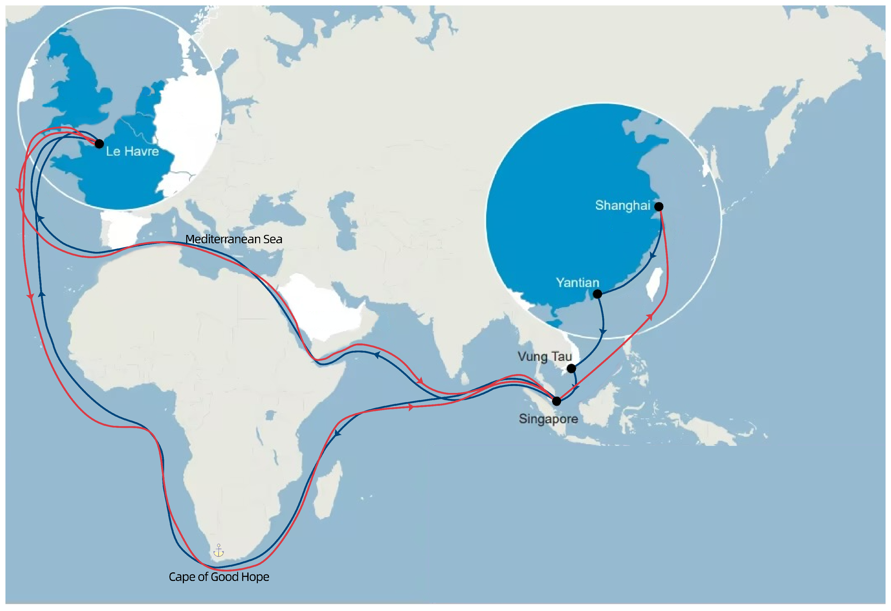
We have selected a route from Asia to northern Europe, specifically the route between Shanghai in China and Le Havre in France (https://www.cma-cgm.com/products-services/flyers, accessed on 1 September 2023). In the eastward direction, there are two options: one route passes through the Mediterranean, known as the SECA region, and the other route navigates around the Cape of Good Hope. Similarly, in the westward direction from Shanghai to Le Havre, there are two possibilities: one route takes the path through the Mediterranean, the SECA region, while the other option involves circumnavigating the Cape of Good Hope.

The comprehensive details of these routes can be found in Figure 4.

Simultaneously, referring to [45], we present the total distances traveled by each route through SECA and non-SECA as follows (

Table 1. The distances of different routes within different areas.

Sub-Model	The Total Distance of Eastward within SECA (nm)	The Total Distance of Eastward within Non-SECA (nm)	The Total Distance of Westward within SECA (nm)	The Total Distance of Westward within Non-SECA (nm)
NN	–	13,787	–	14,190
NE	–	13,787	1915	8808
EE	1915	8405	1915	8808

) (nm denotes the nautical mile, which serves as the unit of measurement for distances).

4.1.2. Parameter Settings

Initially, we establish the parameter values to generate fundamental outcomes, and subsequently, we shall perform a comprehensive sensitivity analysis to assess the impacts of these parameters. Enumerated below are the respective considerations and values:

1.

The fixed cost c. Referring to [46], we first set $c=\$\mathrm{360,000}$ per week for a 20,000-TEU (Twenty-foot Equivalent Unit) container ship.

2.

The MGO price $\gamma$. Referring to [47], we set $\gamma$ to be an average value of 1000 ($/tonne).

3.

The LSFO price $\beta$. Referring to [48], we set $\beta$ to be an average value of 700 ($/tonne).

4.

The total number of available vessels in the vessel company X is set to 40 [49].

5.

Referring to [36], we set $f\left(v^3\right)=0.00086\times v^3,a=0.00086$.

6.

Referring to [50], we set $v_{max}=18$ knots.

7.

We set the $Delta=0.00001$.

4.2. Basic Results

Through our experimentation utilizing the routes outlined in Figure 4, we have conducted numerical assessments, and the obtained results are presented in

Table 2. Basic results.

Sub-Model	NN	NE	EE
x	10	9	8
$v_1^{\mathrm{G}}$ (knot)	18.00	18.00	–
$v_2^{\mathrm{G}}$ (knot)	18.00	–	–
$v_1^{\mathrm{M}\text{-}\mathrm{NECA}}$ (knot)	–	–	18.00
$v_1^{\mathrm{M}\text{-}\mathrm{ECA}}$ (knot)	–	–	9.88
$v_2^{\mathrm{MNECA}}$ (knot)	–	18.00	18.00
$v_2^{\mathrm{M}\text{-}\mathrm{ECA}}$ (knot)	–	7.42	9.88
$t_1^{\mathrm{G}}$ (hour)	765.94	765.94	–
$t_2^{\mathrm{G}}$ (hour)	788.33	–	–
$t_1^{\mathrm{M}\text{-}\mathrm{NECA}}$ (hour)	–	–	466.94
$t_1^{\mathrm{M}\text{-}\mathrm{ECA}}$ (hour)	–	–	193.86
$t_2^{\mathrm{MNECA}}$ (hour)	–	489.33	489.33
$t_2^{\mathrm{M}\text{-}\mathrm{ECA}}$ (hour)	–	256.72	193.86
MGO cost ($)	–	91,638.47	321,405.56
LSFO cost ($)	5,456,857.90	4,407,109.56	3,357,361.22
Fixed cost of vessels ($)	3,600,000	3,240,000	2,880,000
Total cost ($)	9,056,857.90	7,738,748.04	6,558,766.78

. In Table 2, NN, EN, NE, and EE refer to the optimal solutions of model [M3-NN], model [M3-EN], model [M3-NE], model [M3-EE], respectively. Given that both model [M3-NE] and model EN have identical distances for SECAs and non-SECAs, the only discernible difference lies in the choice of the route direction through SECAs. Consequently, the model settings remain fundamentally similar, and thus, we have opted for model [M3-NE] as our experimental choice for now. Model [M3-EN] can be examined in reference to the experimental results obtained from model [M3-NE].

In a comprehensive evaluation taking into account factors such as fuel costs and route distances, it is evident that the model [M3-EE] (which selects the routes passing through the Mediterranean Sea from Shanghai to Le Havre and from Le Havre to Shanghai) exhibits the lowest overall cost of 6,558,766.78 USD, representing the optimal decision made in consideration of multiple factors. Regarding vessel speed, it is manifestly clear that a ship’s speed is slower when traversing the SECAs compared to the non-SECAs. As described in Section 2, ships utilize MGO when passing through SECAs, which has a higher cost compared to LSFO used in non-SECAs. Additionally, ship speed and fuel consumption exhibit a cubic relationship. Consequently, shipping companies opt to reduce vessel speed in SECAs to minimize fuel costs. Furthermore, the ship travel time increases with longer distances. As evident from the table, the model [M3-NN] results in the longest travel distances and hence the longest travel times as ships navigate around the Cape of Good Hope in both eastbound and westbound directions. Conversely, under the model [M3-EE], ships pass through the Suez Canal, resulting in shorter travel distances and the shortest travel time. In terms of the number of deployed ships, greater distances correspond to a higher number of deployed ships. This is because, under certain speed constraints, longer distances lead to increased travel times, necessitating the deployment of a greater number of ships to ensure the fulfillment of weekly service frequency requirements. Therefore, the model [M3-NN] exhibits the highest deployed ship quantity with 10 vessels, while the model [M3-EE] has the lowest with 8 vessels.

It is worth noting that due to changes in the decision-making processes related to shipping company voyage routes, the ETA for vessels is subject to alterations. In other words, the introduction of the new policy will also precipitate shifts in operational decisions made by shipping companies.

4.3. Sensitivity Analysis

As concerns surrounding ${\mathrm{SO}}_{\mathrm{x}}$ emissions from shipping continue to escalate, an increasing number of countries and organizations are proposing a series of measures to limit ${\mathrm{SO}}_{\mathrm{x}}$ emissions from vessels, such as the establishment of SECAs. Consequently, the prices of LSFO and MGO are undoubtedly subject to fluctuations, thus impacting the optimal decisions of shipping companies. Furthermore, in fundamental analysis, certain critical parameters, such as the weekly fixed cost per ship, are typically assumed to be deterministic. However, in reality, these parameters often experience dynamic fluctuations. Therefore, conducting sensitivity analyses becomes essential to examine the effects of these parameters on operational decisions while considering their dynamic nature in real-world scenarios.

4.3.1. Impact of the MGO Price

This study primarily focuses on investigating the impact of MGO price $\gamma$ on operational decisions. Given the growing emphasis on ${\mathrm{SO}}_{\mathrm{x}}$ emissions problems and sustainable development, the MGO price has emerged as a crucial tool for carbon emission control, significantly influencing the decisions of shipping companies. Hence, the value of $\gamma$ is subject to change in practice, necessitating a sensitivity analysis of this parameter. In this experiment, we consider a range of MGO prices from $900 to $2500 per tonne.

The computational results are summarized in Figure 5, which reveals several noteworthy findings. Firstly, from the total cost perspective, both the model [M3-NE] and model [M3-EE] exhibit an upward trend in total cost with an increase in MGO prices. It is noteworthy that the model [M3-NN], as it does not utilize MGO, remains unaffected by variations in MGO prices, resulting in a constant cost. Moreover, as MGO prices rise, ship speeds decline. To meet the requirements of weekly service frequency, shipping companies will deploy more vessels, consequently leading to an increase in the fixed cost of vessels. Correspondingly, as the number of vessels deployed increases, ship speeds decrease, resulting in cost reduction, as exemplified by the model [M3-EE] in Figure 5. (The model [M3-EE], having the longest distance traveled using MGO, is most sensitive to MGO price changes, exhibiting more pronounced cost fluctuations in response to MGO price variations.)

4.3.2. Impact of the LSFO Price

Within the framework of fundamental analysis, the deterministic assumption prescribes a fixed value of 700 dollars/ton for the LSFO price ($\beta$). However, to incorporate the inherent volatility observed in real-world scenarios, this sensitivity analysis considers a range of values for $\beta$, encompassing a spectrum from $200 to $900 per ton. Computational results are summarized in Figure 6.

In general, when the LSFO price increases, the total costs for the model [M3-EE], model [M3-NE], and model [M3-NN] all rise. Due to the relatively high proportion of distances covered using LSFO in all three models, the impact of LSFO price variations on the total costs is more pronounced compared to the effect of MGO price changes on individual models. Specifically, the total cost increase is primarily driven by the rise in LSFO costs. Furthermore, as the distance covered using LSFO increases, the LSFO costs become more susceptible to LSFO price fluctuations. Notably, in the provided Figure 6, the model [M3-NN] experiences the fastest escalation in both total costs and LSFO costs, while the model [M3-EE] demonstrates the slowest rate of cost escalation.

4.3.3. Impact of the Weekly Fixed Cost per Ship

This study specifically focuses on investigating the impact of the weekly fixed cost per ship on operational decisions. A predetermined value of $360,000 is initially assigned to the weekly fixed cost per ship. However, it should be noted that the value of c is subject to significant variations due to various factors, such as the repercussions of epidemics or unforeseen circumstances, and it may even experience increasing prices owing to technological advancements, such as becoming equipped with advanced scrubbers [33]. Consequently, a range of values for c is defined, spanning from 340,000 to 600,000 dollars, and the corresponding outcomes are documented in Figure 7.

In a broader context, the total costs for all models increase with the rise of the weekly cost per ship c. Specifically, as c increases, the fixed cost of vessels continuously grows across all models. However, when the fixed cost per ship becomes excessively high, shipping companies reduce the number of vessels deployed. At this point, the variation in the fixed cost of vessels depends on the trade-off between the cost increase caused by rising ship unit prices and the cost reduction resulting from a decrease in the number of vessels. As indicated in Figure 7, there is a slight decline in the fixed cost of vessels when c reaches 680,000. Simultaneously, due to the reduction in the number of vessels, ships will augment their sailing speed to meet the required service frequency, resulting in an increase in fuel costs, as demonstrated by the rise in MGO costs for the EE model in Figure 7. (Since the model [M3-EE] has already reached the maximum speed for LSFO sailing, its costs remain unaffected by changes in the number of vessels deployed.)

5. Conclusions

This research delves into the implications of designating the Mediterranean as an SECA and its impact on the decision-making processes of shipping companies. The study focuses on determining optimal route choices, optimal sailing speeds, and optimal deployment quantities of vessels for each route. Initially, we developed a complex MINLP model. Subsequently, based on the route preferences of shipping companies, we divided the model into four sub-models. Utilizing piecewise-linear functions to approximate the nonlinear function, we transformed the model into four MILP models for solution.

Through meticulous experiment, our proposed model has demonstrated its efficiency, leading to several notable conclusions: (i) In our experiments, considering factors such as route length and fuel prices, shipping companies ultimately chose routes passing through the Mediterranean region, both in eastward and westward directions. (ii) Regarding sailing speeds, ships navigated at slower speeds in SECAs compared to non-SECAs. This is due to the higher price of MGO fuel used in SECAs compared to the LSFO used in non-SECAs. Additionally, fuel consumption is cubicly related to sailing speed. Consequently, to reduce fuel costs, ships reduce their sailing speeds while traversing SECAs. (iii) With regard to vessel deployment quantities, longer voyage distances necessitate a higher number of ships deployed to meet weekly service frequency requirements. Furthermore, we analyzed the impact of varying fuel prices and the weekly cost per ship on various cost components in each sub-model. Generally, an increase in these factors led to an overall increase in total costs across the sub-models. Specifically, when MGO prices rise, ships lower their sailing speeds in SECAs. To maintain the required weekly service frequency, shipping companies deploy more ships, resulting in an increase in fixed vessel costs, while fuel costs may decrease due to reduced fuel consumption resulting from lower sailing speeds. Additionally, the sensitivity of cost variations across the sub-models to MGO price changes becomes more pronounced as the length of the SECA routes increases. In another scenario, when the weekly cost per ship increases, shipping companies may reduce the number of vessel deployments (when fixed vessel costs are too high) and increase sailing speeds (to meet weekly service frequency requirements). As a result, the fixed vessel costs may decrease, while fuel costs may increase.

Moreover, this study also offers reference and insights for the IMO when establishing SECAs. In essence, when delineating the specific regions to be designated as SECAs, it becomes imperative to consider not only the local ramifications of SECA implementation on carbon and sulfur emissions but also to delve into the region’s distinct attributes. Factors such as whether it serves as a pivotal maritime hub and how the introduction of policies may sway the route selection choices of shipping companies are facets requiring meticulous scrutiny. An all-encompassing assessment of the environmental implications is essential, facilitating the formulation of judicious and scientifically grounded decisions. This, in turn, advances the cause of fostering a greener and more sustainable trajectory for the maritime industry.

Meanwhile, our study does come with limitations. As articulated in our analysis of basic results, the designation of the Mediterranean as an SECA policy will exert influence on shipping companies’ decision-making processes. In our research, we primarily focus on the long-term impact of this policy on shipping companies, addressing strategic issues such as route selection in planning. Concurrently, alterations in decisions related to shipping routes and other factors will necessitate adjustments in the ETA, thereby affecting the short-term decisions of these companies. Hence, in future research endeavors, we aim to refine our analysis to encompass the policy’s influence on short-term company decisions, specifically addressing operational concerns.

In summary, our study constitutes a substantial contribution to the understanding of how shipping companies can make judicious decisions in response to the recent policy initiatives introduced by the IMO. It possesses a strong timeliness and practicality, rendering it highly applicable in contemporary contexts. Through a comprehensive analysis of various optimal decision changes undertaken by these shipping companies, such as alterations in routes leading to shifts in fuel consumption patterns and fuel types, we subsequently examine the overall carbon and sulfur emissions. This enables us to assess the policy’s holistic environmental impact, thereby furnishing the IMO with a robust foundation for crafting more scientifically grounded decisions, thus fostering the advancement of the maritime industry toward a greener and more environmentally sustainable trajectory.