Article

Modeling and Solution Algorithm for Green Lock Scheduling Problem on Inland Waterways

1
School of Traffic and Transportation Engineering, Central South University, Changsha 410075, China
2
School of Engineering, Deakin University, Waurn Ponds, VIC 3216, Australia
*
Author to whom correspondence should be addressed.
Mathematics 2024, 12(8), 1192; https://doi.org/10.3390/math12081192
Submission received: 8 March 2024 / Revised: 8 April 2024 / Accepted: 13 April 2024 / Published: 16 April 2024

Abstract

:
Inland navigation serves as a vital component of transportation, boasting benefits such as ample capacity and minimal energy consumption. However, it also poses challenges related to achieving navigation efficiency and environmental friendliness. Locks, which are essential for inland waterways, often cause ship passage bottlenecks. This paper focuses on a green lock scheduling problem (GLSP), aiming to minimize fuel emissions and maximize navigation efficiency. Considering the realistic constraints, a mixed-integer linear programming model and a large neighborhood search solution algorithm are proposed. From a job shop scheduling perspective, the problem is decomposed into three main components: ship-lockage assignment, ship placement subproblem, and lockage scheduling subproblem coupled with ship speed optimization. A large neighborhood search algorithm based on a decomposition framework (LNSDF) is proposed to tackle the GLSP. In this, the complex lockage scheduling problem is addressed efficiently by mapping it to a network planning problem and applying the critical path method. Numerical experiments substantiate the effectiveness of our proposed model and a heuristic approach was used in solving the GLSPs. In the sensitivity analysis, under three different objective weight assignments, the resulting solutions achieved average effective ship fuel savings of 4.51%, 8.86%, and 2.46%, respectively. This indicates that our green lock scheduling problem considering ship speed optimization can enhance ship passage efficiency while reducing carbon emissions.

1. Introduction

In the process of ship navigation, there are many bottlenecks, such as channel navigation problems before entering container ports [1,2], dams [3,4], and canals [5,6] in inland waterway navigation. Locks, as important components in inland waterway transportation, are also one of the major bottlenecks in the navigation process of inland waterway transportation. Developed countries such as China, Europe, and North America have commonly used inland waterways, such as the 29 single-chamber locks upstream of the Mississippi River [7] and the 6 locks along Belgium’s Albert Canal [8]. China’s inland waterways host over 300 locks of various sizes, including large- and medium-sized ones [9]. With the development of inland waterways and the consequent increase in traffic volume, some locks are experiencing capacity constraints, leading to disruptions in waterway operations. Due to the high cost and long construction cycles of inland waterway improvement and new channel crossings, optimizing ship scheduling processes stands out as an effective measure to enhance the efficiency of inland waterway navigation.
To ensure the safe and orderly flow of ships through locks, it is essential to allocate lock chambers for bidirectional ship traffic within the navigation channel. This process, known as lock scheduling, involves determining ship berthing positions within lock chambers and scheduling the start times for each lock. Traditional ship lock scheduling commonly relies on heuristic rules based on engineers’ experience to prioritize ship queues [4,10]. However, such methods lack scientific rigor and comprehensive consideration, especially in situations of heavy ship traffic, making effective scheduling difficult to achieve. Research on lock scheduling can be categorized into single lock scheduling and serial locks scheduling. The study by Passchyn et al. [11] found that the single lock of the parallel chambers scheduling problem for optimizing ship waiting times is strongly NP-hard even without considering the ship placement problem. Verstichel et al. [12] systematically considered the necessary constraints of the ship placement problem and proposed an improved best-fit heuristic two-dimensional packing algorithm to solve the ship placement problem, and the numerical simulation results showed that the heuristic algorithm has a high efficiency. Subsequently, the team utilized branch-and-bound [13] logic-based Benders decomposition [14] to solve the small-scale single-lock scheduling problem with parallel chambers accurately. But, these two accurate algorithms still struggle to solve the large-scale single lock of the parallel chambers scheduling problem effectively. Ji et al. [15] regarded this problem as a coupled problem of the vehicle routing problem with ship placement scheduling and proposed an adaptive large neighborhood search and an improved best-fit algorithm. His study marked the first successful attempt to efficiently solve the large-scale single-lock scheduling problem with parallel chambers.
Inland waterways in China often leverage stepped channelization to enhance navigation conditions, resulting in the wide-spread distribution of serial locks. Studies have demonstrated that the joint scheduling of serial locks can maximize the overall capacity and service levels [16,17]. Compared with the single lock scheduling problem, the ship flow routes in the serial-lock system are more diverse, and the scheduling schemes of adjacent locks affect each other, so the serial-lock scheduling problem has a higher complexity. In China, there are more abundant scheduling studies for the Three Gorges-Gezhou Dam (TGD). Yuan et al. [18] divided the TGD lock scheduling into three subproblems: lock allocation, schedule optimization, and the ship scheduling problem, and proposed a chaotic embedded particle swarm optimization algorithm to solve it. Zhang et al. [3] proposed a multi-objective mathematical model for optimizing lock utilization, the average waiting time, and ship energy consumption in the joint scheduling problem of the TGD. They introduced a multi-objective metaheuristic algorithm (MOMA) based on fuzzy correlation entropy for solving it. Subsequently, Zheng et al. [19] further considered the impact of the Three Gorges ship lift and approach channel on the scheduling of the TGD, and proposed a collaborative adaptive multi-objective algorithm (CAMOA) for solving it based on this foundation. All of the above studies conducted in-depth research on the navigation efficiency and green carbon emission objectives of the scheduling problem of the TGD locks, but only the special staircase lock structure of the TGD was not generalized.
In terms of the general serial-lock scheduling problem (SLSP), Smith et al. [7] developed a discrete event simulation model for the passage of ships through five locks on the upper reaches of the Mississippi River. Prandtstetter et al. [20] introduced a variable neighborhood search approach for optimizing the scheduling of the nine-lock system along the Austrian segment of the Danube River. Passchyn et al. [21] proposed a mixed-integer linear programming model (MILP) with time-indexing and lockage-indexing for the SLSP. They evaluated the efficacy of the CPLEX solution model on a small-scale instance, confirming its efficiency. They analyzed the impact of scheduling rules such as first-come-first-served (FCFS) and shortest lockage service time priority, as well as the expansion and capacity enhancement of locks, on ship passage efficiency. However, the above studies did not consider the ship placement subproblem, instead simplifying this subproblem into a knapsack problem and a one-dimensional packing problem.
Ji et al. [22] addressed this subproblem in SLSP, developing an MILP for the general SLSP from the perspectives of flexible job shop scheduling. They employed Gurobi for the exact solution of the model, and the results indicated that the model constructed from the job shop scheduling perspective exhibited a higher efficiency. Furthermore, Ji et al. [23] proposed a decomposition algorithm framework for solving the general serial-lock scheduling problem. They introduced a heuristic solving algorithm combining a large neighborhood search and dynamic programming, effectively addressing large-scale serial-lock scheduling problems. Additionally, they analyzed the impact of factors such as ship priorities and uneven lockage capacities.
All of the previously mentioned studies aimed to improve ship crossing efficiency or lock chamber utilization without considering the environmental factors of lock scheduling. In recent years, with the continuous growth of the waterway transport volume and the increasing advocacy of the concept of low-carbon transportation, more and more scholars have focused on the problem of ship speed optimization in shipping. Unlike previous studies that usually regarded the navigation time of ships between water hubs as a parameter, these scholars considered ship speed as a variable and explored the interplay between the efficiency of navigation and the cost of “green” and low-carbon transportation [6,24]. Defryn et al. [25] focused on the passage of a single ship through a single lock and investigated the impact of optimizing the speed of a single ship on other ships from a game theory perspective. Tan et al. [26] and Buchem et al. [27] investigated the joint schedule design and speed optimization problem for a inland waterway service using different approaches, but both focused on only one ship. Passchyn et al. [21] studied the passage of ships through a serial-lock system with a single chamber. They developed a ship-lockage assignment model based on time discretization and analyzed the impact of optimizing ship speeds on the total ship staying time and carbon emissions. Golak et al. [28] focused on ships passing through a serial-lock system, assuming the uninterrupted continuous operation of the locks. They constructed an MILP to optimize the total ship staying time and carbon emissions. It is worth noting that this study assumed the continuous and uninterrupted operation of the locks, with fixed start times for lockage, which may not align with real-world scheduling scenarios. Yang et al. [5] proposed a nonlinear model with two linear approximation methods to optimize the overall cost of ship navigation from the perspective of system optimization, and the experimental results showed the necessity and effectiveness of considering the green objectives for ship navigation strategies. However, the aforementioned studies utilized overly simplified descriptions of chamber capacity, failing to address the actual ship placement issues.
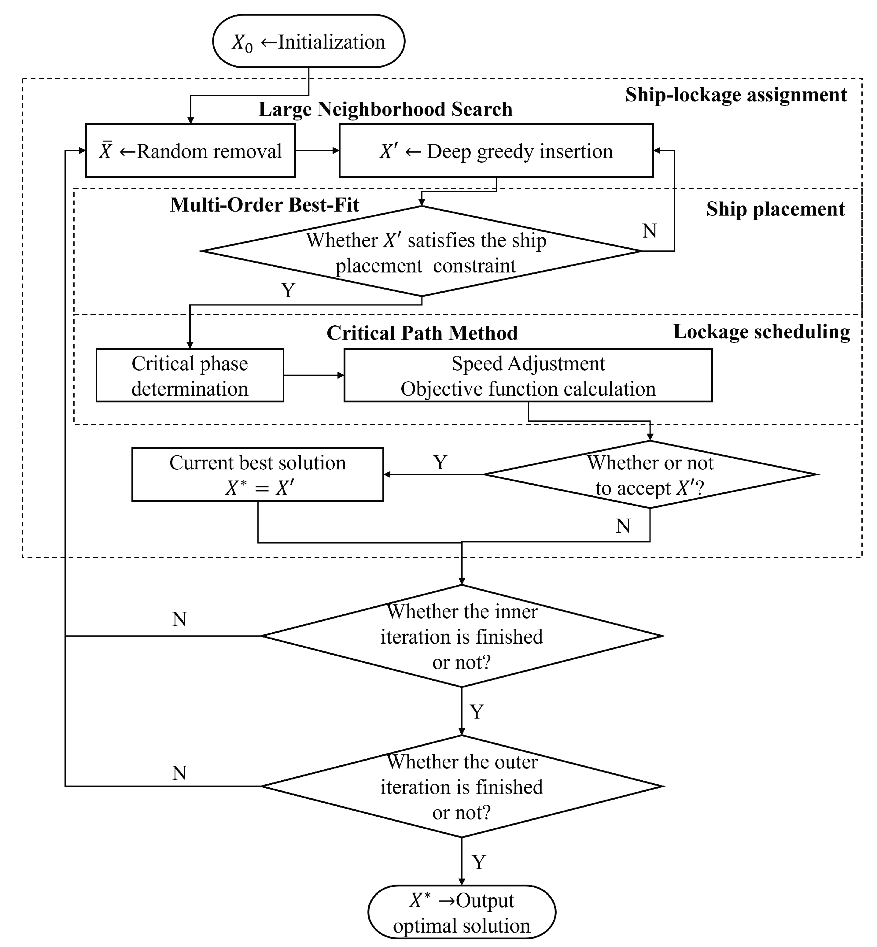
This paper investigates the green lock scheduling problem (GLSP) of ships traveling bidirectionally through serial locks, considering features such as ship placement and ship speed optimization. The objective was to minimize both total fuel emissions and total ship staying time. To address this, an MILP was constructed based on job shop scheduling theory. To efficiently solve large-scale GLSPs, the problem was decomposed into subproblems including lockage scheduling, ship placement, and ship-lockage assignment. A large neighborhood search algorithm based on a decomposition framework (LNSDF) is proposed. An innovative approach was taken to map the complex lockage scheduling subproblem, which considers ship speed optimization, into a network planning problem. The critical path method (CPM) was then employed to solve this mapped problem efficiently. Numerical experiments demonstrated that the MILP proposed in this paper can be accurately solved using CPLEX for small-scale GLSPs. Additionally, large-scale problems can be effectively resolved by the LNSDF. The sensitivity analysis indicates that the GLSP model can ensure ship passage efficiency while effectively reducing ship fuel emissions.

2. Problem Description

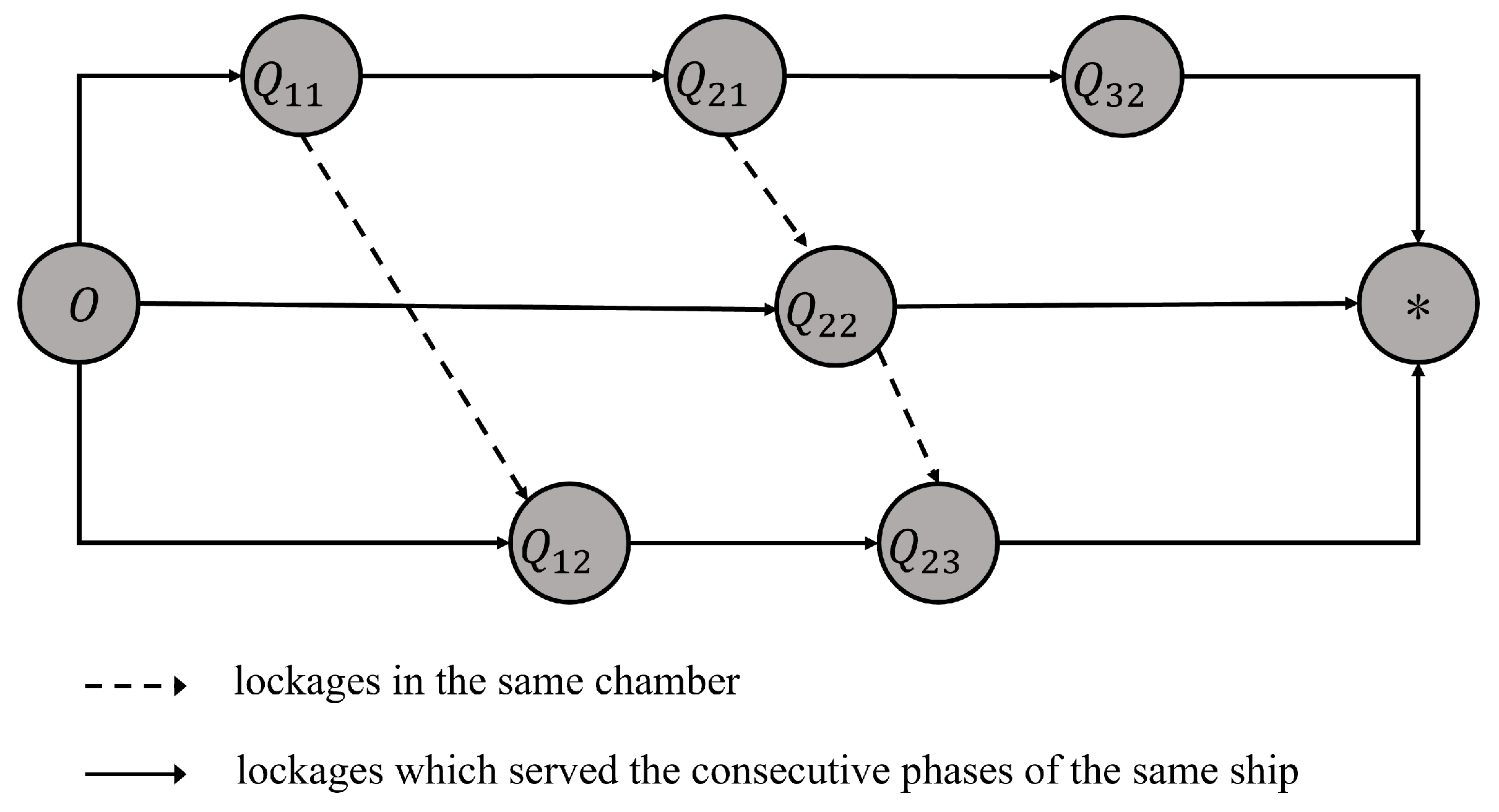
The green lock scheduling process studied in this paper is illustrated in 
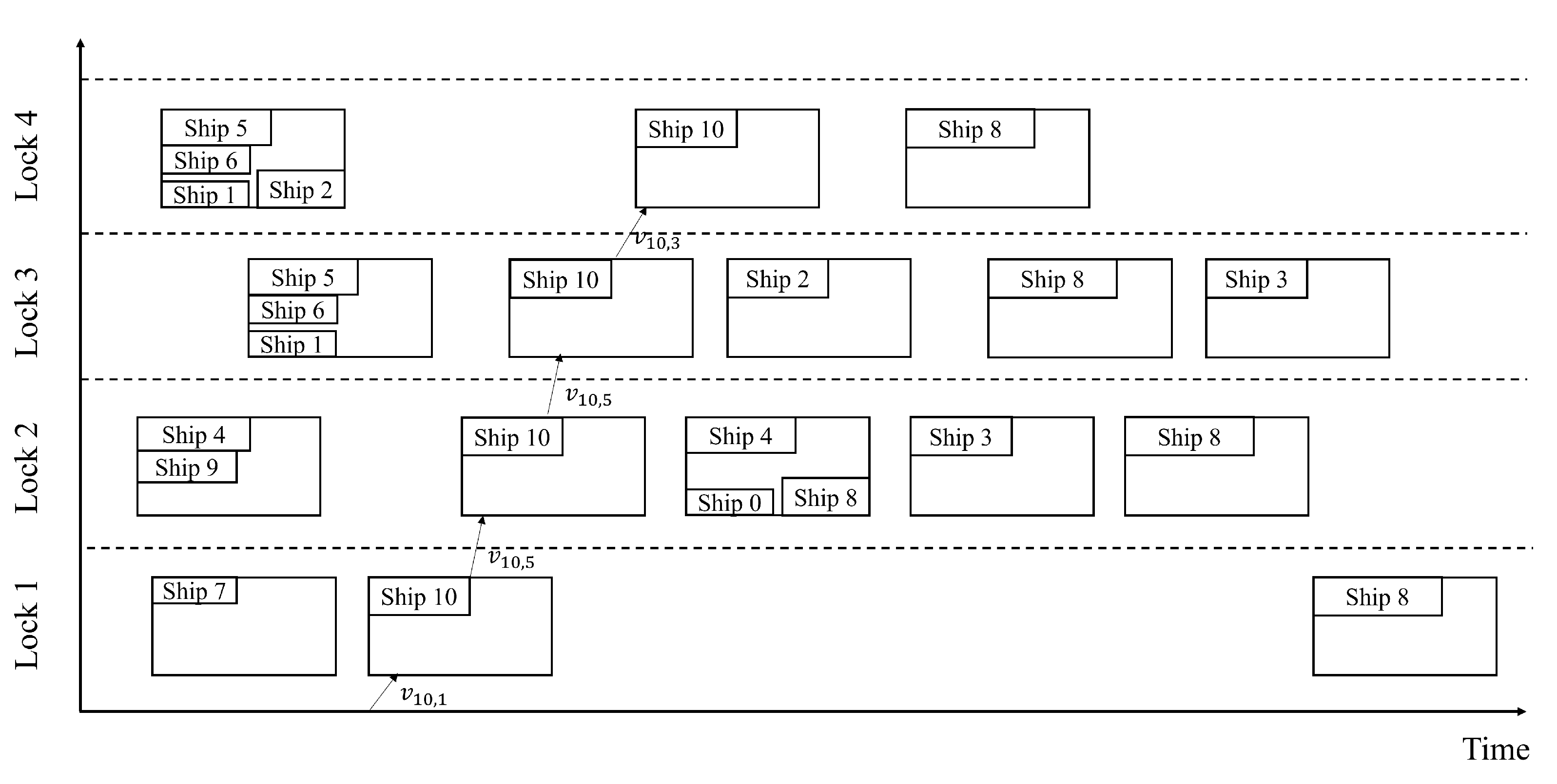
Figure 1. Several locks are distributed along the inland waterway, with each chamber being able to both provide passage services for ships traveling upstream and downstream. The properties of each chamber include its length, width, draft, and the operational time for a lockage. An additional empty lockage is required between two consecutive lockages in the same direction within the same chamber. On the waterway, there is a bidirectional flow of ship traffic distributed across different times and spaces. Ships each have fixed routes to enter or leave the series-lock systems via the main channel or tributaries. The declared information of the ship includes the length, width, locks it needs to pass, draft, tonnage, speed range, and distance to the first lock. In the scheduling process of the GLSP, the lock operator needs to make decisions on three key aspects: the allocation of ships and lockages, the determination of the optimal arrival speed of ships and the optimal opening time of lockages, and the two-dimensional placement of ships in the lock chambers. These decision-making processes are referred to as the ship-lockage allocation problem, the lock scheduling problem, and the ship placement problem, respectively. Factors to be considered throughout the decision-making process include the characteristics of each lock chamber, the declaration information provided by the ships, the two-way ship traffic flow in the channel, and operational constraints. The goal is to develop a lock operation schedule that maximizes lock efficiency and minimizes ship fuel consumption.
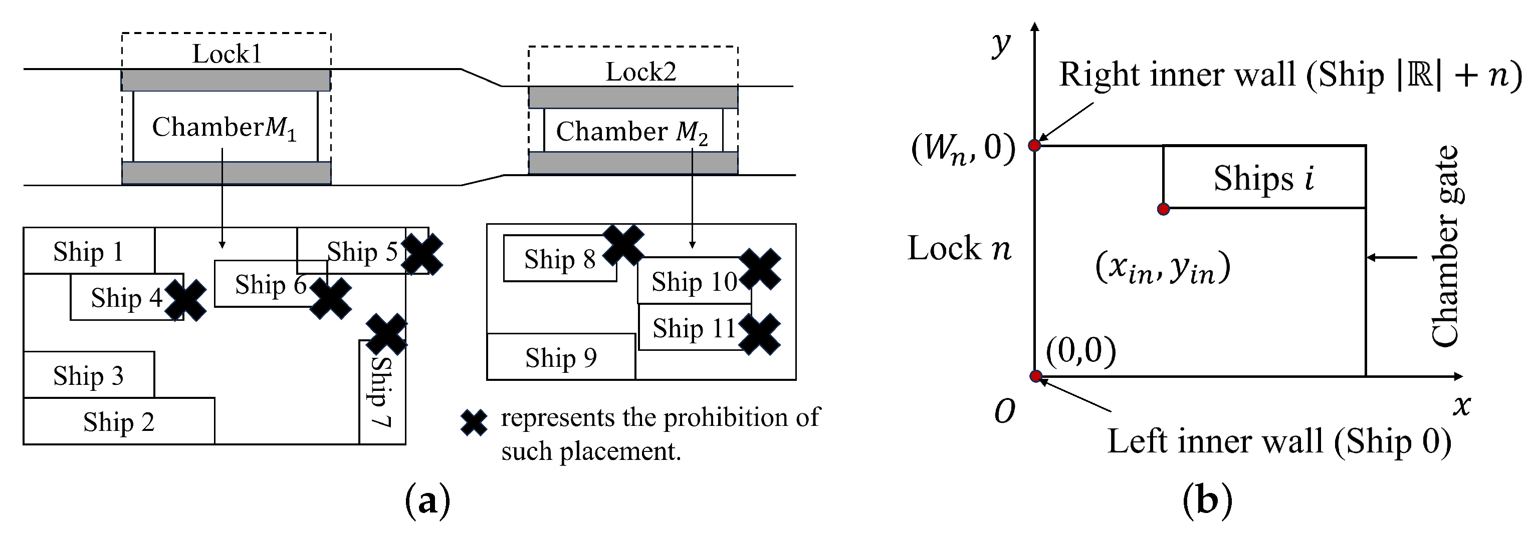
Therefore, based on these factors, the spatio-temporal constraints, such as ship attributes, lock characteristics, and operational limitations, need to be considered when addressing the GLSP. Among these, the ship placement problem requires the two-dimensional arrangement of ships within the lock chamber to be resolved. Apart from the typical two-dimensional packing constraints, safety mooring constraints for ships within the lock chamber also need to be taken into account. Specifically, as shown in Figure 2a, besides meeting the two-dimensional packing rigidity constraint, any ship must be moored against the inner wall of the chamber or be completely moored alongside a longer ship [12], which will be described by the model constraints in Section 3.

3. Proposed GLSP Model

In the GLSP, the scheduling of locks is influenced by both adjacent locks and ship speeds. Additionally, ship routes exhibit diverse characteristics, making the problem description complex. This paper maps the problem into a job shop scheduling problem, introducing ship speed optimization features and fuel emission objectives to construct the GLSP model. Specifically, ships are treated as jobs, locks as machines, and the process of ships passing through multiple locks sequentially is viewed as the processing of jobs across different machines. The ability of a lock to serve multiple ships simultaneously is considered as the machine having the batch processing capability.
The basic assumptions of the model are as follows:
  • Safety margins are incorporated within the dimensions of the ships;
  • The depth of the chambers meets the draft requirements of all ships;
  • The ships navigate at a constant speed within each voyage segment.

3.1. Symbol Description

The significance of the symbols involved in the mixed-integer linear programming model (MILP) is as shown in Table 1.

3.2. Optimization Objectives

For the operator of the locks, improving the efficiency of lock operations to ensure ships pass through as quickly as possible is its primary goal. For the ships, they aim to minimize fuel consumption (carbon emissions) during their journey. Therefore, the GLSP considers both ship passage efficiency and ship fuel emissions as two objectives. Specifically, maximizing ship passage efficiency is described by minimizing the total ship staying time in the serial-lock system, as shown in Equation (1).
f 1 = i R π i ( c i I | N i | r i )
In elucidating the correlation between ship speed and fuel consumption, we draw on the derivations and assumptions outlined in [27]. When sailing, a ship encounters resistance R proportional to the square of its speed v 2 . Accordingly, the power required (denoted by P) can be expressed as the product of the resistance, i.e.,  P ( v ) = R ( v ) v . Subsequently, from the fact that fuel consumption per unit of time is proportional to the power required, the formula for fuel consumption per unit of ship can be derived as F ( v ) = α v 3 , where α represents the ship’s fuel consumption coefficient. Furthermore, considering that the time required for a ship to sail a distance D is t = D / v , we can derive the fuel consumption for sailing a distance D as F ( v , D ) = α D v 2 . This result is consistent with the findings of [21] and confirms our analysis. Due to the nonlinear constraints introduced by the speed variable, we discretize the ship’s speed and introduce a binary variable τ i n v to linearize the objective as Equation .
f 2 = i R n N i ( α i D i n v V i ( v 2 τ i n v ) )
In this paper, the problem is transformed into a single-objective optimization problem using weighted coefficients, and the objectives are normalized. This is represented by Equation .
min k 1 f 1 F m i n 1 + k 2 f 2 F m i n 2

3.3. Constraints

The model constraints consist of three components: ship-lockage assignment (Contraints (4)–(7)), lockage scheduling (Contraints (8)–(15)), and ship placement (Contraints (17)–(39)).
Constraints (4)–(7) are the relevant constraints for ship-lockage assignment.
q L n u δ i n q = 1 , n N , i R n u
q L n d δ i n q = 1 , n N , i R n d
z n q δ i n q , n N , i R n , q L n
z n q i R n δ i n q , n N , q L n
Constraints (4) and (5) indicate that each ship must be serviced by exactly one lockage at each lock, and the direction of the lockage must be consistent with that of the ship, respectively. Constraints (6) and (7) ensure that each activated lockage serves at least one ship.
Constraints (8)–(15) are constraints related to lockage scheduling.
C n q P n q a i n + C m a x δ i n q 1 , n N , i R n , q L n
c i n C m a x δ i n q 1 + C n q , i R , n N i , q L n
c i n C m a x 1 δ i n q + C n q , i R , n N i , q L n
Constraint (8) indicates that each lockage can only start operating after the ship it serves arrives. Constraints (9) and (10) specify that ships must depart from the lock after the corresponding lockage has finished operating.
a i I i 1 = r i + D i I i 1 v V i v τ i , I i 1 , v , i R
a i I i j = c i I i , j 1 + D i I i j v V i v τ i , I i j , v , i R , j < | N i |
v V i τ i n v = 1 , i R , n N i
Constraints (11) and (12) represent that the arrival time of a ship at the lock is determined by the distance between the ship and the lock and the ship’s speed on that segment, where v ¯ denotes the reciprocal of the ship’s speed, and  D i I i 1 represents the distance traveled by the ship until reaching the first ship on the route. Constraint (13) states that each ship selects only one average speed for sailing on a segment.
C n q C n p + 2 C m a x β n p q P n p + λ n p q , n N , p , q L n
C n p C n q + 2 C m a x 1 β n p q P n q + λ n p q , n N , p , q L n
P n q p n z n q , n N , q L n
Constraints (14) and (15) represent the temporal sequence relationship between the adjacent lockage within the same lock. The subsequent lockage must wait for the completion of the preceding lockage before it can begin. If the consecutive lockages have the same direction, an empty lockage is required between them. Constraint (16) specifies that the processing time of each lockage is determined by the properties of the chamber where it is assigned.
Constraints (17)–(38) are the constraints related to ship placement, wherein Constraints (17)–(21) are standard two-dimensional constraints used to prevent ship placement from exceeding the dimensions of the lock chamber, and Constraints (22)–(38) are special ship mooring constraints for lock scheduling.
e i j n + e j i n + b i j n + b j i n + 1 δ i n q + 1 δ j n q 1 n N , i , j R n , q L n
x i n x j n + W e i j n W w i , n N , i , j R n
y i n y j n + L e i j n L l i , n N , i , j R n
x i n + w i W n + 1 δ i n q W , n N , q L n , i R n
y i n + l i L n + 1 δ i n q W , n N , q L n , i R n
In the ship placement problem, we first need to consider the constraints of the standard 2D crate, i.e., (1) the ship cannot overlap inside the lock chamber, which is modeled by constraints (17)–(19)), and (2) the ship cannot be placed beyond the 2D dimensions of the lock chamber, which is modeled by (20) and (21).
y j n y i n 1 ξ i j n L , n N , i R n , j R i n
y i n y j n l j l i + 1 ξ i j n L , n N , i R n , j R i n
Constraints (22) and (23) indicate that ship i can only be moored to the left of ship j, whose length is greater than ships i in R i n . The  R i n is the set of ships that can be moored by ship i in lock n. The ships in R i n must simultaneously satisfy the following conditions: they are in the same direction as ship i and need to pass through the lock n that ship i needs to pass through.
x j n x i n w i + 1 ξ i j n W , n N , i R n , j R i n
x j n x i n w i 1 ξ i j n W , n N , i R n , j R i n
Constraints (24) and (25) denote another condition for the mooring of ships i and j, i.e., ship j must be adjacent to ship i in lock n.
x | R | + n , n x i n w i + 1 ξ i , | R | + n , n W , n N , i R n
x | R | + n , n x i n w i 1 ξ i , | R | + n , n W , n N , i R n
A ship may be moored to the left side of the right wall of the lock chamber in addition to the left side of other ships, as indicated by constraints (26) and (27). Specifically, the right inner wall of the lock chamber of lock n is represented by a virtual ship | R | + n , whose position is fixed as ( W n , 0 ) , where | R | represents the number of ships planned during the planning period.
y j n y i n 1 μ i j n L , n N , i R n , j R i n
y i n y j n l j l i 1 μ i j n L , n N , i R n , j R i n
x j n x i n w i + 1 μ i j n W , n N , i R n , j R i n
x j n x i n w i 1 μ i j n W , n N , i R n , j R i n
x 0 n x i n w i + 1 μ i 0 n W , n N , i R n
x 0 n x i n w i 1 μ i 0 n W , n N , i R n
Similarly, when ship i needs to be moored to the right of ship j, the spatial relationship is ensured by Constraints (28)–(31). Constraints (32) and (33) indicate that, besides other ships within the lockage, ship i can also be moored to the right of the left wall of the lock chamber, represented by a virtual ship 0, with its coordinates fixed at (0,0).
i R n , j R i n ξ i j n + μ i j n + ξ i , | R | + n , n + μ i 0 n 1 , n N , i R n
ξ i j n + μ j i n 1 , n N , i j , i , j R n
Constraint (34) ensures that each ship must be moored on one side of either another ship or the lock chamber. When two ships of equal length are present, they are likely to be moored to each other (e.g., ships 10 & 11 in Figure 2a). This violates the safety mooring requirement in practical scheduling, and Constraint (35) is set to prevent this situation.
δ j n q δ i n q η i j , n N , i j , i , j R n , q L n
δ i n q δ j n q η i j , n N , i j , i , j R n , q L n
ξ i j n + μ i j n η i j , i R n , n N , j R i n
Constraints (36)–(38) indicate that two ships that do not transfer through the same lockage cannot moor to each other.
a i n a j n ω i j n C m a x , n N , i j , i , j R n
a i n a j n ω i j n 1 C m a x , n N , i j , i , j R n
c i n c j n ω i j n C m a x , n N , i j , i , j R n
c i n c j n ω i j n 1 C m a x , n N , i j , i , j R n
In practical lock operation scheduling, the FCFS principle may be employed. This means that within the same lock, ships that arrive earlier should depart before ships that arrive later. This is represented by Constraints (39)–(42).
0 a i n C m a x , i R , n N i
0 c i n C m a x , i R , n N i
0 C n q C m a x , n N , q L n
0 P n q P m a x , n N , q L n
x i n 0 , . . , W , y i n 0 , , L , n N , i R n
δ i n q 0 , 1 , i R , n N , q L n
ξ i j n , μ i j n , e i j n , b i j n 0 , 1 , n N , i , j R n
β n p q 0 , 1 , n N , p , q L n
τ i n v 0 , 1 , i R , n N i , v V i
Constraints (43)–(51) are type and range constraints for the variables.
z n , q + 1 z n q , n N , q , q + 1 L n
C n , q + 1 C n q , n N , q , q + 1 L n
To speed up the model, Constraints (52) and (53) are added to enforce the order of use and start times for lockages within the same chamber.

4. Solution Method

4.1. Solution Framework

In order to solve large-scale GLSP problems efficiently, we propose a large neighborhood search algorithm based on the decomposition framework (LNSDF). Considering the high complexity of the GLSP, we decomposed the GLSP into an allocation main problem with two subproblems (i.e., the ship-lockage allocation main problem, the ship placement subproblem, and the lockage scheduling problem) based on the problem characteristics. Subsequently, effective solution methods were applied for each problem to realize the interactive solution of the three problems.
As shown in Figure 3, LNSDF is a method that applies a decomposition framework on the basis of LNS, with interactions between various subproblems. The ship-lockage allocation problem, as the main problem, influences the determination of ship placement and lockage scheduling schemes. Therefore, initially, the removal and insertion operators of LNS are employed to reorganize the allocation relationship between ships and lockages, a heuristic that obtains new allocation schemes. Subsequently, the two-dimensional placement of ships in each lockage is carried out, using the well-established Multi-Order Best-Fit (MOBF) method to make decisions on ship placement schemes. At this stage, if MOBF fails to find any feasible placement schemes, the objective function value of the current solution is set to infinity, and the solution will not be adopted. Next, for feasible solutions, decisions are made on ship speed schemes and lockage start times. In this subproblem, two decision variables of the objective function can be obtained: the ship speed and lockage opening schedule (the time when ships leave the lock system), and then the objective function value is calculated, obtaining a feasible new solution.
As for the lock scheduling problem, the start time of each lock is not only affected by the timing of other locks, but also by the ship speed. Therefore, the difficulty in solving the lock scheduling subproblem lies in how to optimize the ship speed while obtaining the optimal opening scheme of the locks. To this end, we innovatively map this problem to a network planning problem and use the critical path method (CPM) to solve it.
X = Ω 1 ( 1 ) Ω 1 ( q ) Ω 1 L 1 Ω n ( 1 ) Ω n ( q ) Ω n L n Ω N ( 1 ) Ω N ( q ) Ω N L N
In LNS, it is crucial to first define the structure of the solution for the problem. For ease of representation, ships will be divided into several ship phases based on the locks they need to pass through. Each phase will be assigned to a lockage in the lock it passes through. This paper designs the solution structure as shown in Equation (54), where Ω n ( q ) represents the set of phases assigned to lock n’s lockage q.
The basic approach to solving the problem is to reconstruct the solution structure using removal and insertion operators to generate feasible solutions. During the removal process, to avoid repetitively removing the same ship passage in iterations, a tabu list is used to store the removed ship passages. These removed ship phases are not removed again for a certain tabu tenure. During the insertion process, the lockage’s compliance with ship placement constraints and other relevant spatiotemporal constraints is verified to ensure the feasibility of the reconstructed solution structure. With the obtained solution structure, the CPM is employed to decide the optimal start time for ships and lockages, taking into account ship speeds. Subsequently, the solutions are evaluated, and the acceptance of these solutions is determined using solution acceptance rules. This iterative process aims to seek an optimized solution and can be described using Algorithm 1.
Algorithm 1: The solution framework of LNSDF
Mathematics 12 01192 i001

4.2. Initialization

A heuristic method is used to generate an initial solution. For each lock, a separate lockage is assigned to each ship phase that needs to pass through it. The ship speed is set to its minimum value for each ship. This process results in an initial solution structure where ship speed information is determined.
Treating lockages as nodes and the minimum interval between lockages as edges, the initial solution structure can be represented as a network graph. By considering the temporal relationships between lockages, the shortest path algorithm can be employed to determine the optimal start time for each lockage. This provides the objective function value for the initial solution. Specific descriptions are in Section 4.4.2.

4.3. Removal and Insertion

LNS was first proposed by Shaw and Paul [29] for solving vehicle path problems, and has been widely used in engineering fields. In addition to the vehicle path problem, LNS and its derivative adaptive large neighborhood search (ALNS) have shown their superb global search ability in discrete combinatorial optimization problems such as port berth scheduling [30] and flexible job shop scheduling [31]. Based on the characteristics of the problem, this paper constructs a tabu-based random removal operator and a deep greedy insertion operator to reconstruct the solution structure.
For ease of presentation, we divide the process of navigating a ship between the serial-lock systems into a number of phases, each of which represents only the ship’s situation within a particular lock. The removal and insertion operations we perform next are both performed on the ship phases.

4.3.1. Random Removal

To enhance the diversity of the solution structure, a random removal operator is used to randomly remove a certain number ( ρ ) of ships from the lockages in the current solution structure.To prevent the repetitive and inefficient removal of the same ship phases, a tabu strategy is added. Specifically, there is a 50% chance that the removed phases will be added to the tabu list, and they will be released after a certain number of iterations. After removing a portion of phases from solution X, a temporary solution X ¯ is obtained.

4.3.2. Deep Greedy Insertion

The deep greedy insertion operator, initially proposed by Ropke et al. [32] to solve vehicle routing problems, is adapted in this paper for the GLSP. The basic idea is to compute the objective function value for all possible insertion positions of the removed phases into the temporary solution X ¯ , considering all feasible insertion locations.The determination conditions for the feasible positions are as follows: Some of these constraints are implicitly satisfied by the setup of the solution structure (Contraints (6) and (7)). The other part of the constraints requires feasibility determination, such as the operation constraints (Constraints (4) and (5)) and the ship placement constraints.
If the lockage to be inserted is an existing lockage, it is necessary to determine whether all the ships in the lockage satisfy the ship placement constraints (Constraints (17)–(38)). If the insertion violates these constraints, the objective function value is set to infinity. The best insertion position and corresponding objective function value for each removed phase are recorded. Then, phases are inserted into their optimal positions in descending order of the objective function value, resulting in a new solution X .
The feasibility check for ship placement is achieved through MOBF. This algorithm was initially proposed by Verstichel et al. [33] for solving the ship placement problem and has been proven to have good computational efficiency. The key purpose of the MOBF algorithm is to determine the lock chamber arrangement scheme for the given lockage by sorting the ships based on width, length, or area, and adjusting gap sizes after each placement to maximize the safe and efficient placement of ships within the lock chamber. Algorithm 2 describes the specific steps of the deep greedy insertion operator.
Algorithm 2: Deep Greedy Insertion
Mathematics 12 01192 i002

4.4. Lockage Scheduling Subproblem

With sailing speed as a parameter to customize the inputs, lockage scheduling at a serial-lock system can be described as a shortest-path problem, and finding the optimal start time of lockages can be translated into finding the shortest path [23]. However, in the GLSP, ships’ speed is considered a variable, so this approach cannot be directly applied to the GLSP. Therefore, from the perspective of job shop scheduling, each ship’s transit through a lock is analogized to a workpiece’s processing step, with lockage representing a batch of these processing steps. The fuel consumption incurred during the ship’s journey is the resource consumption during the process. As a result, lock scheduling, considering speed optimization, is mapped to the job shop scheduling problem, considering the balance of resource consumption. The problem is described and a network planning diagram is constructed, followed by its resolution using the critical path method (CPM) [34].
The constraints to be considered in the lockage scheduling problem are Constraints (8)–(15)).

4.4.1. Ship Speed Decision

The process of speed decision-making involves three steps: determining critical ship phases, adjusting speed, and relaxing time constraints.
  • Determining critical ship phases
In the solution structure X, associations are established between the phases and the lockage. Using the lockages as vertices and the ship sailing and lockage operation processes as arcs, we can derive several paths. Among them, the longest duration path starting from the earliest starting lockage and ending at the latest ending lockage is termed the critical path. The lockages involved in this path are referred to as critical lockages. The latest ship phase to arrive at the critical lockage is termed a critical phase.
As shown in Figure 4, path Q 11 Q 22 Q 23 Q 14 represents the longest duration critical path, and the latest arrival ship phases s 21 , s 22 , s 12 , s 72 of critical lockages on this path are termed critical phases. This process is mapped to a network planning problem, and the critical lockages, as well as the critical ship phases that affect the overall lockage efficiency, are determined by using the CPM.
The specific steps for determining critical lockages and ship critical phases using the critical path method are as follows.
Step 1 Construct the network graph. Based on the relationship between serviced ships and lockages, a double-labeled network graph is constructed, as seen in Figure 5. Except for the start node (0) and the end node (*), each node represents the end time of each lockage, and the arcs describe the operation process of subsequent nodes representing the lockage. The weight of the arcs represents the duration of the corresponding operation for the lockage. The arcs in the graph include two types: arcs connecting two lockages, which served the consecutive phases of the same ship ( A 1 ), and arcs connecting two consecutive lockages in the same chamber ( A 2 ).
Step 2 Compute the weights of each arc as follows. The weight of arcs in set A 1 is the sum of the sailing time and the lockage processing time (as seen in the first and second equation of Equation (55)), and the weight of arcs in set A 2 is the sum of the lockage interval time and the processing time (as seen in the third equation of Equation (55)).
t m p , n q = max D i n v V i v τ i n v , m p = 0 , q L n , n = I i 1 , i R max c i m + D i n v V i v τ i n v + P n q , p L m , q L n , m , n N , i R λ n p q + P n q , m = n , p < q , p , q L n , n N 0 , n q =
where t m p , n q represents the arc weight connecting node Q m p to node Q n q , which denotes the duration of the corresponding operation, c i m denotes the departure time of ship i from lock m, λ n p q represents the switching time between lockage p and lockage q in lock n, and P n q is the processing time of lockage q in lock n.
Step 3 Use forward pass calculations to determine the earliest start and finish times E S n q for each node in the network graph (see Equation (56)), and employ backward pass calculations to determine the latest start and finish times L F n q for each node in the network graph (see Equation (57)). Let C n q F denote the set of predecessors connected to node Q n q , and C n q B denote the set of successors connected to node Q n q .
E S n q = max p C nq B E S n q + t p , n q , q L n , n N 0 , n q = 0
L F n q = max p C nq F L F n q t n q , p , q L n , n N E S n q , n q =
Step 4 Determine critical lockages and ship phases. In Step 3, R n q represents the range of time that can be adjusted without affecting the overall duration (see Equation (58)). A lockage with R n q = 0 is considered a critical lockage. The phase with the latest arrival time in the critical lockage is identified as the critical phase in that lockage. The path consisting of arcs corresponding to R n q = 0 in critical lockages forms the critical path. If the arc corresponding to R n q = 0 in a critical lockage belongs to A 2 , then the corresponding critical phase is a virtual phase. The final set of critical phases obtained is denoted as S .
R n q = L F n q E S n q , q L n , n N
2.
Adjusting Speed
After obtaining S through the CPM, adjustments need to be made to the sailing speeds of each critical phase to reduce the completion time of the planning horizon and enhance the overall efficiency of serial-lock system. Clearly, phases with the potential to achieve greater efficiency with fewer resources should be prioritized for speed adjustments. Let us assume that v i k and v i k + represent the initial speed and the speed after accelerating once, respectively, for phase k of ship i, k S . The contribution of each phase to the objective function value, denoted by ϕ k , is calculated based on Equations (59). By evaluating ϕ k , the sailing speeds of the critical phases are increased successively while ensuring that the critical lockages remain unchanged, until all critical phases reach their maximum speeds or just before the critical lockages change.
ϕ k = f 1 X v i f 1 X v i + f 2 X v i + f 2 X v i
3.
Relaxing Time Constraint
After adjusting the sailing speeds of critical phases, it is necessary to examine whether there is any redundant resource usage, i.e., whether ships are waiting. This process is known as time relaxation. Unlike adjusting the sailing speeds, this process does not affect the start times of lockages. As mentioned earlier, the arrival time of critical phases determines the start time of their corresponding lockages. Therefore, non-critical phases may experience some waiting time upon arrival at the corresponding lockage. By reducing the sailing speed of non-critical phases, the waiting time can be converted into the sailing time, reducing fuel consumption.
This process involves traversing all non-critical phases in each lockage. First, non-critical phases with a non-zero waiting time and current speeds not at the minimum speed are identified. Subsequently, the speed of these phases is adjusted to the next lower level. If reducing the speed leads to an increase in the objective function value or renders the current solution infeasible, the reduction is abandoned, and the original sailing speed is retained.

4.4.2. Objective Calculation

The GLSP has two objectives: the total ship’s staying time in the lock system and the total ship’s fuel consumption, which are determined by two decision variables: the time a ship leaves the last lock ( c i I | N i | , i R ) and the ship’s speed ( τ i n v , i R , n N ), respectively.
In Section 4.4.1, we obtained the ship’s speed scenario, which allows us to calculate the ship’s total fuel consumption, and the ship’s total staying time, which needs to be determined by making a decision on the lockage start time. If a ship’s speed is known, the decision of lockage start time for the current solution X structure can be transformed into a shortest path problem. The Bellman–Ford algorithm [35] can be used to solve it.
Specifically, a graph G = ( V , A ) is used to represent the solution structure, as shown in Figure 6. Here, V represents the set of vertices (i.e., lockages) in the solution structure; A represents the sets of arcs between vertices, where solid lines represent arcs between lockages serving the same ship, and dashed lines represent arcs between lockages in the same chamber but occur sequentially. The weights of the arcs correspond to both the sailing time between two lockages for a ship and the switching time ( λ n p q ) between two lockages. Therefore, deciding the start time for each lockage is equivalent to solving a shortest path problem, which can be achieved using the Bellman–Ford algorithm, thereby obtaining the objective function value of the solution structure.

4.5. Acceptance Criteria

Each new solution X obtained after the disruption and repair operations applied to each solution X uses the exponential Monte Carlo acceptance criterion [36] to determine whether it should be accepted. Considering the large-scale optimization capability of the LNS, when F V ( X ) < F V ( X ) , the new solution will be accepted. Inferior solutions will be accepted with a probability of e ϖ ( F V ( X ) F V ( X ) ) , where ϖ is the coefficient controlling the probability of accepting new solutions that are worse than the current one.

5. Numerical Experiments

5.1. Instance Introduction

5.1.1. First Instance Class

This class of instances utilizes the serial-lock instance proposed by Ji et al. [22] for numerical simulation experiments. The configuration of chambers in the locks is shown in Table 2, while the specific ship data are presented in Table 3. Specifically, there are four locks in total. The number of ships varies between 10 and 20, with an average arrival interval ranging from 5 to 30 min. It is assumed that the ship speed can be decided within the range of [15, 20], and the ship speed decision segment includes the first 10 km before reaching the first lock. There are a total of 16 scenarios comprising different proportions of upstream and downstream ships and varying average arrival intervals for each ship size.

5.1.2. Second Instance Class

This class of instances utilizes the instances proposed by Ji et al. [22]. The lock attributes parameters are the same as in Table 2, with the main difference lying in the number of locks and the average arrival interval of ships, as shown in Table 4. Specifically, there are three locks in total. The number of ships varies between 10 and 20, with the average arrival interval ranging from 1 to 30 min. It is assumed that the ship speed can be decided within the range of [12, 15], and the ship speed decision segment includes the first 10 km before reaching the first lock. For each group of different numbers of ships, 10 instances are generated by changing the upstream and downstream traffic ratios and the average arrival interval, resulting in a total of 20 instances.
All experiments in this paper were conducted on a computer equipped with an Intel(R) Core (TM) i5-1340P CPU and 16GB of RAM. The MILP and LNSDF were implemented using CPLEX 12.6.3 and C language, respectively.

5.2. Parameter Setting

This paper utilized the Irace software package developed by López-Ibáñez M et al. [37] to determine the parameters and settings of LNS. The basic principle is to provide a set of representative instances and a set of possible values for each parameter. Then, using an iterative racing method, combinations of parameter values are adjusted to approach the optimal solution as closely as possible.
The method involves three steps:
  • Randomly sampling parameters within a specific range, with the probability of selection following a specific distribution;
  • Comparing the sampled parameters and selecting the current optimal configuration based on the performance of the objective function values;
  • Updating the current optimal parameters and repeating the experiments until the stopping conditions are met. For each of the two instance classes, one instance is randomly selected for applying the sampled parameters, with the objective weights set at k 1 = 0.6 , k 2 = 0.4 .
All instances are run 20 times under the same set of parameters, ultimately outputting a set of optimal parameters, as shown in Table 5.

5.3. Experiment of GLSPs

This section of the experiment utilizes the first instance class and conducts experiments for four different sets of objective weights: k 1 = 0.8 , k 2 = 0.2 , k 1 = 0.6 , k 2 = 0.4 , k 1 = 0.4 , k 2 = 0.6 , and k 1 = 0.2 , k 2 = 0.8 . The experiments consider the FCFS principle for ships, where the importance weight for all ships ( π i , i R ) is 1, and the ship fuel consumption coefficient ( α i , i R ) is 1.049.
To facilitate a clearer comparison between the performance of the LNSDF method and the deterministic method, this study contrasts the average objective function values obtained by MILP and LNSDF over 20 computations. Additionally, to provide a more intuitive comparison of their solutions, the concept of relative deviation (RD) is introduced (see Equation (60)), where F V LNSDF ( i ) represents the objective function value obtained by the LNSDF algorithm in the i-th computation.
R D = i = 1 20 F V L N S D F ( i ) F V M I L P / F V M I L P
The comparison results between MILP and LNSDF under various lockage configurations are shown in Table 6 and Table 7. In all 16 instances, MILP could optimally solve eight small-scale instances, with an average computation time of 3751.04 s. However, as the size of the instances increased, the solving time required by MILP rapidly escalated. When the number of ships exceeded 10, MILP failed to obtain the optimal solution within two hours. In contrast, the proposed algorithm (LNSDF) could achieve high-quality solutions in a shorter time. The average differences between LNSDF and MILP under various objective weights were −0.37%, −0.56%, −0.88%, and −0.83%, respectively. The results of the instances indicate that LNSDF can obtain superior solutions to MILP in a shorter amount of time.
A comparison of the solution obtained using MILP solving with the lower bound of the solution and the LNSDF algorithm is given in Figure 7. First, the results of MILP and LNSDF were similar or equal in some instances. With the four objective weight configurations, MILP was able to optimally solve the algorithm for all 10 ships with a Gap value of 0. With the 20-ship algorithm, the solutions and the lower bounds of MILP and LNSDF were very close to each other in the instances of 5 and 10 min ship intervals, suggesting that both methods are able to find a similar optimal solution in these instances. However, the Gap values of MILP with its lower bound were relatively more significant in the arithmetic case of ship arrival time of 15 vs. 30 min, and the results with LNSDF were more divergent. This was more evident in the objective configuration with weights k 1 = 0.6 , k 2 = 0.4 and k 1 = 0.6 , k 2 = 0.4 . This may be due to the fact that when the ship arrival time interval is close to or more than 1 unit of lockage operation time, it is more difficult for MILP to balance the two objectives of ship speed and lock crossing efficiency when scheduling lockages. When dealing with complex integer programming problems, the CPLEX branch-and-bound algorithm searches the entire solution space to find the optimal solution. However, due to the NP difficulty of integer programming problems, searching the entire solution space can be very expensive and there may be a large number of branches and constraints in the solution space. This may result in the inability to find a globally optimal solution in a given time, thus producing a significant difference from the lower bound.
In this case, the LNSDF algorithm found a solution similar to the MILP algorithm in a more advantageous solution time, which demonstrates the ability of the LNSDF to efficiently solve larger scale GLSPs. In addition, the lower bound of the solution provides valuable information compared to the solution. If the solution of the MILP or LNSDF algorithm is close to or equal to the lower bound of its corresponding solution, this indicates that the resulting solution may be close to the optimal solution.
From Figure 8, it can be observed that, as the weight of the fuel emission objective k 2 increased, the overall fuel consumption of ships gradually decreased, indicating that the scheduling scheme tended to prioritize the low-fuel objective. In practical scheduling processes, the operators of lockage facilities can adjust the weights of different objectives according to different traffic scenarios. When the lockage capacity is insufficient, greater weight can be given to the lockage efficiency objective to ensure ships pass through the lockage as quickly as possible. Conversely, greater weight can be given to the fuel emission objective to minimize ship fuel emissions while ensuring smooth ship passage conditions. Figure 9 gives a schematic diagram of the optimal solution for instance 5_10_0.3, which contains the ship-lockage assignment information, lockage opening time information, ship speed information, and ship placement information, demonstrating that the proposed MILP with the LNSDF is capable of proposing an effective and high-quality solution to the practice GLSP.

5.4. Sensitivity Analysis

This section analyzes the impact of ship importance weights and ship speed on the GLSP without considering the FCFS constraint (i.e., constraints (40)–(43)).

5.4.1. Impact of Ship Importance Weights

This section of the experiment utilized the second instance class conducting experiments under two different sets of objective weights ( k 1 = 0.8 , k 2 = 0.2 , k 1 = 0.2 , k 2 = 0.8 ). The importance weight of ships π i was randomly generated among the values 1, 2, and 3, reflecting the priority of ships in passing through the locks. The ship’s staying time and fuel consumption under each objective weight scenario are illustrated in Figure 10. As shown in Figure 10a,c, in the scenario where k 1 = 0.8 and k 2 = 0.2 , out of the 20 instances, 16 instances had the highest fuel consumption for ships with an importance weight of 3. Additionally, ships with higher importance weights tended to have lower average staying times. This is because, under an emphasis on the efficiency of ship passage through the locks, ships with higher importance weights were prioritized, leading them to travel at higher speeds, thus increasing their carbon emissions during navigation. Figure 10b,d illustrate that, under the scenario where k 1 = 0.2 , k 2 = 0.8 , the priority of ships with an importance weight of 3 was not significantly pronounced. Compared to ships with lower weights, the fuel consumption of ships with an importance weight of 3 was relatively low. This is because, with the increase in k 2 , the scheduling scheme tended to prioritize the low-fuel objectives of ships. In actual scheduling operations, the operators of lock systems can assign different importance weights to different types of ships based on different scenarios. When the lock system is operating at capacity, ships with higher importance weights can be given priority passage.

5.4.2. The Impact of Ship Speed Optimization

In these experiments using the second instance class, we aimed to verify the impact of considering speed optimization on GLSP scheduling solutions. We conducted comparative experiments between LNSDF-NSO (LNSDF without speed optimization, excluding the CPM part) and LNSDF.
To keep the parameters of LNSDF-NSO consistent with those of LNSDF, the navigational distance between all locks was set to 10km, and the decision range of navigational speed was set to 15km/h to 20km/h in LNSDF, which corresponds to the navigational time of the ship between 20 min and 30 min. Since LNSDF-NSO does not adjust the sailing speed, the sailing time of ships obeyed a uniform distribution U ( 20 , 30 ) in LNSDF-NSO.
Then, LNSDF was employed to solve the results of the GLSP under the three objective weighting scenarios: k 1 = 0.2 , k 2 = 0.8 ; k 1 = 0.6 , k 2 = 0.4 ; k 1 = 0.8 , k 2 = 0.2 .
The effectiveness of ship speed optimization was evaluated using the indicator of fuel savings efficiency θ , as defined in Equation (61). Here, f 1 represents the total time ships spent waiting without considering speed optimization, and f 2 is calculated based on the preset travel times obtained without considering speed optimization. f 1 and f 2 then denote the objective values obtained by considering the speed optimization.
θ g k m = f 2 f 2 f 1 f 1 max f 1 , f 1 max f 2 , f 2 2
Table 8 compares the results of LNSDF considering and not considering speed optimization (LNSDF-NSO) under three different objective weight scenarios. The average fuel efficiency savings rates provided by LNSDF for the three solution scenarios were 4.51%, 8.86%, and 2.46%, respectively. This indicates that the ship speed optimization method CPM introduced by LNSDF achieved some effectiveness in reducing ship fuel emissions.
As shown in Table 8, across the three scenarios, the solutions provided by LNSDF achieved ship speed optimization without significantly increasing ship waiting times at the locks, effectively balancing the objectives of ship fuel consumption and waiting time. In the scenario where k 1 = 0.2 and k 2 = 0.8 , the influence of the speed decision operator led to a slight increase in ship waiting times in LNSDF solutions compared to those of LNSDF-NSO. However, the corresponding total fuel consumption of ships decreased. This is because, even when only considering the efficiency of ship passage as the objective, LNSDF still optimizes ship speeds to some extent, reducing fuel consumption.
In the scenario where k 1 = 0.6 and k 2 = 0.4 , the average fuel savings rate of the obtained solutions was highest among the three scenarios. This is because optimizing both ship waiting times and fuel consumption simultaneously can lead to more environmentally friendly ship passage plans without significantly reducing passage efficiency.
In the scenario where k 1 = 0.8 and k 2 = 0.2 , introducing ship speed optimization methods can effectively reduce ship fuel emissions. In practical scheduling, by adjusting scheduling strategies and objective weights, a balance can be achieved between ship fuel consumption and waiting time objectives. This ensures efficient operations while minimizing ship fuel emissions.

6. Conclusions

This study investigates the green lock scheduling problem (GLSP) in the process of ship passage through a serial-lock system. Considering practical factors such as ship placement, an MILP was constructed with the objectives of maximizing lockage efficiency and minimizing ship navigation fuel emissions. To efficiently solve the large-scale GLSP, the problem was decomposed into ship-lockage assignment, lock scheduling, and ship placement subproblems. Based on this problem, a decomposition framework, i.e., a hybrid heuristic solving algorithm called LNSDF, based on the large neighborhood search and critical path method, was proposed.
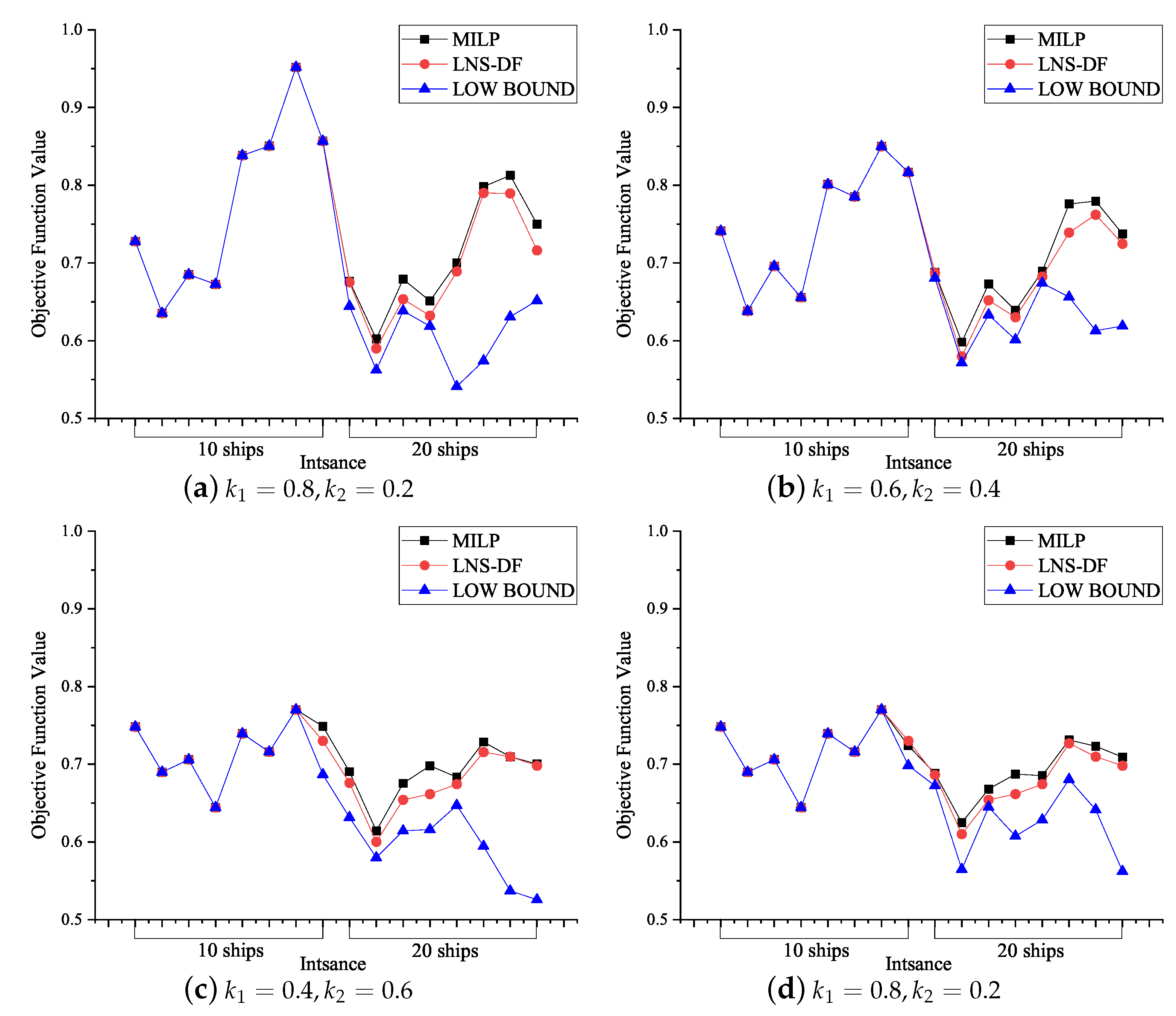
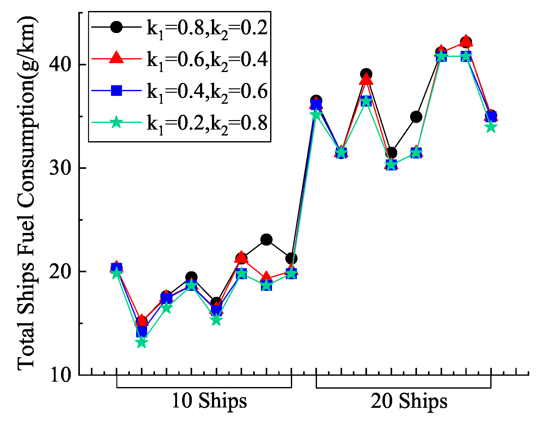
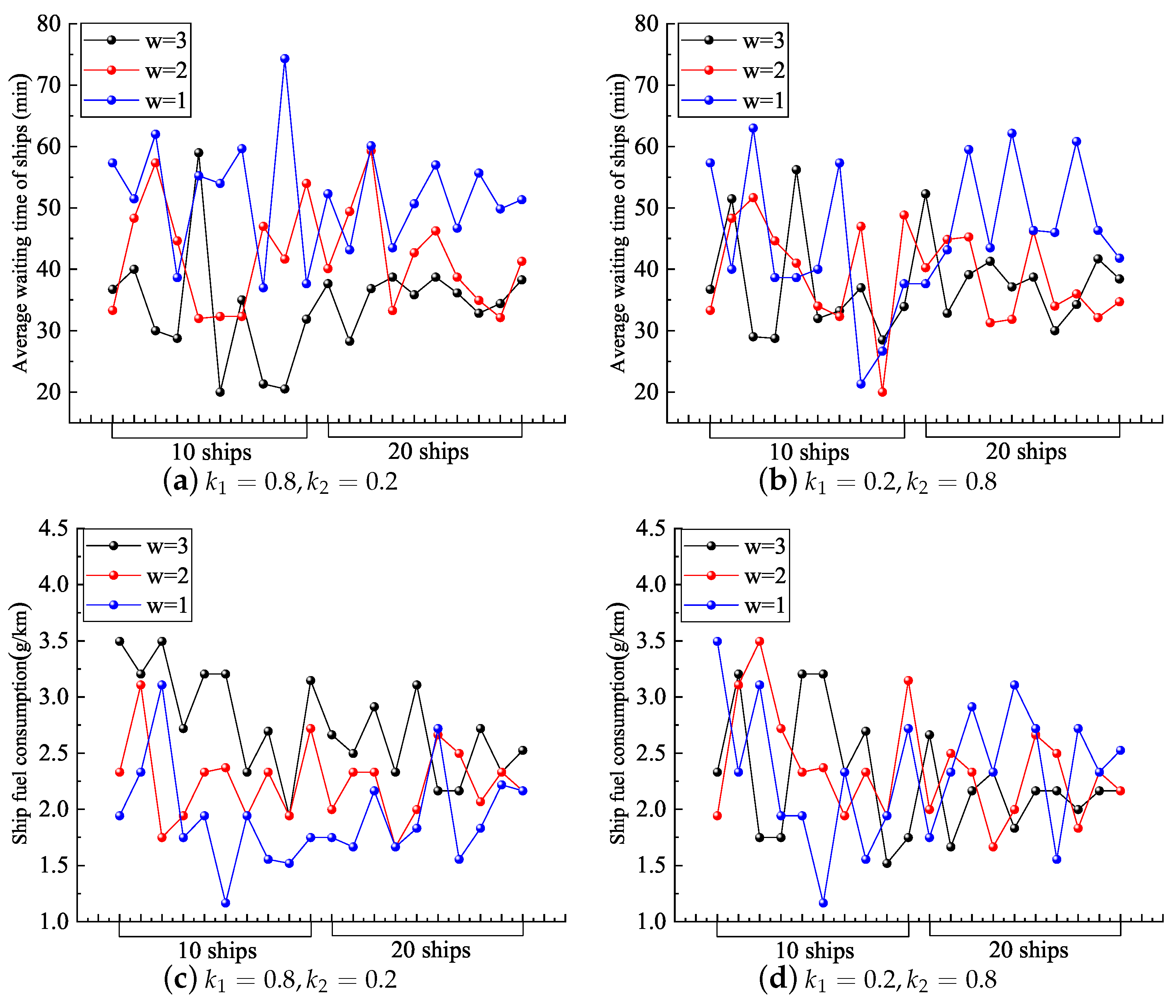
Extensive numerical simulations were conducted to validate the effectiveness of the model and algorithm proposed in this study. The results demonstrate that the MILP proposed in this paper can efficiently solve optimal solutions for small-scale problems using CPLEX. Additionally, LNSDF can achieve high-quality scheduling solutions for larger-scale GLSPs in shorter time frames. Furthermore, considering ship fuel emission objectives can better balance lockage efficiency and ship navigation fuel emissions in different traffic scenarios. Sensitivity analysis results indicate that optimizing ship speed can provide more flexible lockage services. When the lock capacity is insufficient, reducing ship speed can distribute the ship waiting time evenly throughout the navigation process, thereby reducing ship navigation fuel emissions. At the same time, for certain important ships, accelerating navigation can ensure a reduction in the waiting time at the serial-locks system, thereby expediting lockage.
This study is also subject to some limitations. Firstly, the discretization of ship speeds may result in suboptimal solutions due to the limited granularity of the decision space. Secondly, the reliance on weighted optimization for addressing both objectives introduces a significant dependency on the predetermined weights, potentially biasing the obtained solutions. To address these limitations, future research could explore alternative approaches. For instance, employing continuous optimization techniques for ship speeds could enable the exploration of a broader solution space, leading to potentially improved scheduling outcomes. Additionally, the investigation of multi-objective optimization algorithms that do not require predefined weights could offer more candidate solutions.

Author Contributions

Conceptualization, Z.W. and B.J.; methodology, Z.W. and B.J.; software, Z.W.; validation, Z.W. and B.J.; formal analysis, Z.W. and B.J.; investigation, Z.W.; resources, B.J.; data curation, Z.W. and B.J.; writing—original draft preparation, Z.W. and S.S.Y.; writing—review and editing, B.J. and S.S.Y.; visualization, Z.W. and S.S.Y.; supervision, B.J.; project administration, B.J.; funding acquisition, Z.W. and B.J. All authors have read and agreed to the published version of the manuscript.

Funding

This research was funded by National Natural Science Foundation of China, grant number 72371250, and Central South University Graduate Research Innovation Project under Grant No. 1053320222623.

Data Availability Statement

The datasets generated during and analyzed during the current study are available from the corresponding author upon reasonable request.

Conflicts of Interest

The authors declare no conflicts of interest.

References

  1. Jia, S.; Li, C.L.; Xu, Z. Managing navigation channel traffic and anchorage area utilization of a container port. Transp. Sci. 2019, 53, 728–745. [Google Scholar] [CrossRef]
  2. Ji, B.; Huang, H.; Samson, S.Y. An enhanced NSGA-II for solving berth allocation and quay crane assignment problem with stochastic arrival times. IEEE Trans. Intell. Transp. Syst. 2022, 24, 459–473. [Google Scholar] [CrossRef]
  3. Zhang, Y.; Zheng, Q.Q.; He, L.J.; Tian, H.W. Ship traffic optimization method for solving the approach channel and lock co-scheduling problem of the Three Gorges Dam on the Yangzi River. Ocean Eng. 2023, 276, 114196. [Google Scholar] [CrossRef]
  4. Zhang, H.; Ke, J. An Intelligent scheduling system and hybrid optimization algorithm for ship locks of the Three Gorges Hub on the Yangtze River. Mech. Syst. Signal Process. 2024, 208, 110974. [Google Scholar] [CrossRef]
  5. Yang, X.; Gu, W.; Wang, S. Optimal scheduling of vessels passing a waterway bottleneck. Ocean Coast. Manag. 2023, 244, 106809. [Google Scholar] [CrossRef]
  6. Meisel, F.; Fagerholt, K. Scheduling two-way ship traffic for the Kiel Canal: Model, extensions and a matheuristic. Comput. Oper. Res. 2019, 106, 119–132. [Google Scholar] [CrossRef]
  7. Smith, L.D.; Nauss, R.M. Investigating strategic alternatives for improving service in an inland waterway transportation system. Int. J. Strateg. Decis. Sci. (IJSDS) 2010, 1, 62–81. [Google Scholar] [CrossRef]
  8. Verstichel, J.; Vanden Berghe, G. Scheduling Serial Locks: A Green Wave for Waterbound Logistics. In Sustainable Logistics and Supply Chains; Lu, M., De Bock, J., Eds.; Springer International Publishing: Cham, Switzerland, 2016; pp. 91–109. [Google Scholar] [CrossRef]
  9. Zhao, X.; Lin, Q.; Yu, H. A co-scheduling problem of ship lift and ship lock at the Three Gorges Dam. IEEE Access 2020, 8, 132893–132910. [Google Scholar] [CrossRef]
  10. Wang, X.; Qi, H.; Xiao, H.; Zhang, X.; Hu, Y.; Feng, X. Series queuing network scheduling approach to co-scheduling model of three Gorges-Gezhou dam. J. Syst. Sci. Complex. 2010, 23, 715–726. [Google Scholar] [CrossRef]
  11. Passchyn, W.; Coene, S.; Briskorn, D.; Hurink, J.L.; Spieksma, F.C.; Berghe, G.V. The Lockmaster’s Problem. Eur. J. Oper. Res. 2016, 251, 432–441. [Google Scholar] [CrossRef]
  12. Verstichel, J.; De Causmaecker, P.; Spieksma, F.C.; Berghe, G.V. Exact and Heuristic Methods for Placing Ships in Locks. Eur. J. Oper. Res. 2014, 235, 387–398. [Google Scholar] [CrossRef]
  13. Verstichel, J.; De Causmaecker, P.; Spieksma, F.; Berghe, G.V. The Generalized Lock Scheduling Problem: An Exact Approach. Transp. Res. Part E Logist. Transp. Rev. 2014, 65, 16–34. [Google Scholar] [CrossRef]
  14. Verstichel, J.; Kinable, J.; De Causmaecker, P.; Berghe, G.V. A Combinatorial Benders’ decomposition for the lock scheduling problem. Comput. Oper. Res. 2015, 54, 117–128. [Google Scholar] [CrossRef]
  15. Ji, B.; Yuan, X.; Yuan, Y.; Lei, X.; Iu, H.H. An Adaptive Large Neighborhood Search for Solving Generalized Lock Scheduling Problem: Comparative Study with Exact Methods. IEEE Trans. Intell. Transp. Syst. 2019, 21, 3344–3356. [Google Scholar] [CrossRef]
  16. Liu, C.; Qi, J.; Chu, X.; Zheng, M.; He, W. Cooperative ship formation system and control methods in the ship lock waterway. Ocean Eng. 2021, 226, 108826. [Google Scholar] [CrossRef]
  17. Li, X.; Mou, J.; Chen, L.; Huang, Y.; Chen, P. Ship–Infrastructure Cooperation: Survey on Infrastructure Scheduling for Waterborne Transportation Systems. J. Mar. Sci. Eng. 2022, 11, 31. [Google Scholar] [CrossRef]
  18. Yuan, Y.; Ji, B.; Yuan, X.; Huang, Y. Lockage scheduling of Three Gorges-Gezhouba dams by hybrid of chaotic particle swarm optimization and heuristic-adjusted strategies. Appl. Math. Comput. 2015, 270, 74–89. [Google Scholar] [CrossRef]
  19. Zheng, Q.Q.; Zhang, Y.; Guo, W.J.; Tian, H.W.; He, L.J. Solving energy-efficient lock group co-scheduling problem with ship lift and approach channel using a collaborative adaptive multi-objective algorithm. Expert Syst. Appl. 2024, 242, 122712. [Google Scholar] [CrossRef]
  20. Prandtstetter, M.; Ritzinger, U.; Schmidt, P.; Ruthmair, M. A Variable Neighborhood Search Approach for the Interdependent Lock Scheduling Problem. In Evolutionary Computation in Combinatorial Optimization; Ochoa, G., Chicano, F., Eds.; Springer International Publishing: Cham, Switzerland, 2015; Volume 9026, pp. 36–47. [Google Scholar] [CrossRef]
  21. Passchyn, W.; Briskorn, D.; Spieksma, F.C. Mathematical Programming Models for Lock Scheduling with an Emission Objective. Eur. J. Oper. Res. 2016, 248, 802–814. [Google Scholar] [CrossRef]
  22. Ji, B.; Zhang, D.; Samson, S.Y.; Fang, X. An Exact Approach to the Generalized Serial-Lock Scheduling Problem from a Flexible Job-Shop Scheduling Perspective. Comput. Oper. Res. 2021, 127, 105164. [Google Scholar] [CrossRef]
  23. Ji, B.; Zhang, D.; Zhang, Z.; Samson, S.Y.; Van Woensel, T. The Generalized Serial-Lock Scheduling Problem on Inland Waterway: A Novel Decomposition-Based Solution Framework and Efficient Heuristic Approach. Transp. Res. Part E Logist. Transp. Rev. 2022, 168, 102935. [Google Scholar] [CrossRef]
  24. Xie, W.; Xu, S.; Zhang, N.; Liu, J.; Yin, K.; Mao, L. Ship Speed Optimization Method in Canal Environments Considering Waiting Times for Crossing Locks. J. Mar. Sci. Eng. 2024, 12, 375. [Google Scholar] [CrossRef]
  25. Defryn, C.; Golak, J.A.P.; Grigoriev, A.; Timmermans, V. Inland Waterway Efficiency through Skipper Collaboration and Joint Speed Optimization. Eur. J. Oper. Res. 2021, 292, 276–285. [Google Scholar] [CrossRef]
  26. Tan, Z.; Wang, Y.; Meng, Q.; Liu, Z. Joint ship schedule design and sailing speed optimization for a single inland shipping service with uncertain dam transit time. Transp. Sci. 2018, 52, 1570–1588. [Google Scholar] [CrossRef]
  27. Buchem, M.; Golak, J.A.P.; Grigoriev, A. Vessel Velocity Decisions in Inland Waterway Transportation under Uncertainty. Eur. J. Oper. Res. 2022, 296, 669–678. [Google Scholar] [CrossRef]
  28. Golak, J.A.P.; Defryn, C.; Grigoriev, A. Optimizing Fuel Consumption on Inland Waterway Networks: Local Search Heuristic for Lock Scheduling. Omega 2022, 109, 102580. [Google Scholar] [CrossRef]
  29. Shaw, P. Using Constraint Programming and Local Search Methods to Solve Vehicle Routing Problems. In Principles and Practice of Constraint Programming—CP98; Goos, G., Hartmanis, J., Van Leeuwen, J., Maher, M., Puget, J.F., Eds.; Springer: Berlin/Heidelberg, Germany, 1998; Volume 1520, pp. 417–431. [Google Scholar] [CrossRef]
  30. Liu, B.; Li, Z.C.; Sheng, D.; Wang, Y. Integrated planning of berth allocation and vessel sequencing in a seaport with one-way navigation channel. Transp. Res. Part B Methodol. 2021, 143, 23–47. [Google Scholar] [CrossRef]
  31. Cao, S.; Li, R.; Gong, W.; Lu, C. Inverse model and adaptive neighborhood search based cooperative optimizer for energy-efficient distributed flexible job shop scheduling. Swarm Evol. Comput. 2023, 83, 101419. [Google Scholar] [CrossRef]
  32. Ropke, S.; Pisinger, D. An Adaptive Large Neighborhood Search Heuristic for the Pickup and Delivery Problem with Time Windows. Transp. Sci. 2006, 40, 455–472. [Google Scholar] [CrossRef]
  33. Verstichel, J.; De Causmaecker, P.; Berghe, G.V. An Improved Best-fit Heuristic for the Orthogonal Strip Packing Problem. Int. Trans. Oper. Res. 2013, 20, 711–730. [Google Scholar] [CrossRef]
  34. Bishnoi, N. Critical Path Method (CPM): A Coordinating Tool. Int. Res. J. Manag. Sci. Technol. 2018, 9, 459–467. [Google Scholar]
  35. Cormen, T.H.; Leiserson, C.E.; Rivest, R.L.; Stein, C. Introduction to Algorithms; MIT Press: Cambridge, MA, USA, 2022. [Google Scholar]
  36. Ayob, M.; Kendall, G. A Monte Carlo Hyper-Heuristic to Optimise Component Placement Sequencing for Multi Head Placement Machine. In Proceedings of the International Conference on Intelligent Technologies, InTech, Halifax, NS, Canada, 13–17 October 2003; Volume 3, pp. 132–141. [Google Scholar]
  37. López-Ibáñez, M.; Dubois-Lacoste, J.; Cáceres, L.P.; Birattari, M.; Stützle, T. The Irace Package: Iterated Racing for Automatic Algorithm Configuration. Oper. Res. Perspect. 2016, 3, 43–58. [Google Scholar] [CrossRef]
Figure 1. Green lock scheduling diagram.
Mathematics 12 01192 g001
Figure 2. Ship placement diagram. (a) shows the diagram of examples of prohibitions and permissions of ship placement, and (b) shows the diagram of the coordinate.
Mathematics 12 01192 g002
Figure 3. Solution framework for GLSP.
Mathematics 12 01192 g003
Figure 4. Illustration of critical phase.
Mathematics 12 01192 g004
Figure 5. Double-labeled network graph.
Mathematics 12 01192 g005
Figure 6. Schematic diagram of the precedence relations of different lockages. O represents the origin, and * represents the destination.
Mathematics 12 01192 g006
Figure 7. Comparison of upper and lower bounds obtained from CPLEX solution with LNSDF solution.
Mathematics 12 01192 g007
Figure 8. Total fuel consumption of ships with different objective weights.
Mathematics 12 01192 g008
Figure 9. Optimal solution obtained by LNSDF and MILP (5_10_0.3).
Mathematics 12 01192 g009
Figure 10. Impact of ship importance weights on dwell time and fuel consumption with different objectives weights.
Mathematics 12 01192 g010
Table 1. Symbol description of MILP.
Sets
N Set of locks, indexed by n
R Set of ships, indexed by i , j
N i Subset of N , which represents the locks that ship i passes through. | N | represents the number of locks that ship i needs to pass through.
R u , R d Subset of R , which represents the upstream and downstream ships, respectively. R u R d = R , R u R d =
R n Subset of R , which represents the ships passing through lock n
L Set of lockages, indexed by p , q
L n Subset of L , which represents the lockage processed in lock n
L u , L d Subset of L , which represents the upstream and downstream lockages, respectively. L u L d = L , L u L d =
I i I i = ( I i 1 , . . . , I i k , . . . , I i | N i | ) , which represents the sequence of locks that ship i needs to pass through, where I i 1 and I i | N i | is the origin and destination lock of ship i
R i n Set of ships that ship i can be allowed to moor at lock n
V i The discrete speed set of ship i, V i = v m i n i , , v m a x i
Parameters
L n , W n The length and width of chamber in lock n
L , W The maximum length and width among all chambers
l i , w i The length and width of ship i
r i The time when ship i arrives at the serial-lock system
p n The time for processing one lockage (lockage processing time) of chamber in lock n
λ n p q The minimum interval time between lockage p and q in lock n when they are processed in the same chamber. If the directions of p and q are opposite, it is 0; otherwise, it is the empty lock processing time of chamber in lock n
P m a x The maximum processing time among all lock chambers
C m a x The upper bound of the completion time of all ships
D i n Distance that ship i travels from the previous lock (or origin) to lock n
v m i n i , v m a x i The minimum and maximum speed of ship i
π i The importance weight of ship i
α i The fuel consumption coefficient of ship i
Variables
δ i n q Binary variables, indicating whether ship i is processed by lockage q in lock n (1) or not (0)
a i n Continuous variable, indicating the arrival time of ship i at lock n
C i n Continuous variable, indicating the completion time of lockage q in lock n
P n q Continuous variable, indicating the processing time of lockage q in lock n
β n p q Binary variables, indicating whether lockage p in lock n is processed before lockage q (1) or not (0)
z n q Binary variables, indicating whether lockage q in lock n is used (1) or not (0)
c i n Continuous variable, indicating the time when ship i departs lock n
ξ i j n , μ i j n Binary variables indicating whether ship i is moored to the left and right of ship j in lock n (1) or not (0)
e i j n Binary variable indicating whether ship i is completely located to the left of ship j in lock n (1) or not (0)
b i j n Binary variable indicating whether ship i is completely located behind ship j in lock n (1) or not (0)
ω i j n Binary variable, indicating whether ship i arrives at lock n later than ship j (1) or not (0)
η i j n Binary variable, indicating whether ship i and ship j are processed by the same lockage in lock n (1) or not (0)
x i n , y i n Integer variable, indicating the coordinates (horizontal and vertical) of ship i in lock n, Figure 2b illustrates the location of the specific representation
τ i n v Binary variable, indicating whether ship i arrives at lock n with speed v (1) or not (0)
Table 2. Chamber configurations.
Chamber TypeDimension (m2)Processing Time (min)Switching Time (min)
SC 1600 × 13 , 600 1616
LC 2400 × 20 , 000 1616
Table 3. Information of the first instance class.
Lock and Ship Flow ConfigurationsInstance
Number of ships10, 20
Mean inter-arrival time (min)5, 10, 15, 30
Upstream and downstream ratio0.3, 0.5
Range of ship speed (km/h)[15, 20]
The name of instance5-10-0.3
Lock configurationLC-LC-SC-LC
Distance between adjacent locks (km)(10)-10-18-25
Table 4. Information of the second instance class.
Lock and Ship Flow ConfigurationsInstance
Number of ships10, 20
Mean inter-arrival time (min)1, 5, 10, 15, 30
Upstream and downstream ratio0.3, 0.5
Range of ship speed (km/h)[12, 15]
The name of instance1-10-0.3
Lock configurationLC-SC-LC
Distance between adjacent locks (km)(10)-12-18
Table 5. Parameters and settings of the LNSDF.
ParametersDescriptionTuned Value
ρ Removes the degree of destruction in the operatorRandom value in the range of ( 1 , 0.5 ( i R N i R T 1 ) )
ε Reaction factor in weight adjustment process0.1
Ψ Maximum number of LNSDF iterations (outer iteration)20
ψ The maximum number of iterations of inner iteration min ( 50 , max ( R , 20 ) )
ϖ Index threshold parameter of Monte Carlo acceptance criteria0.3
ξ The tabu period of ship phase in the tabu table5
1 R T represents the phase of the ship in the current tabu table.
Table 6. Comparative results of MILP and LNSDF objectives weights of k 1 = 0.8 , k 2 = 0.2 , k 1 = 0.6 , k 2 = 0.4 .
Weight
Instance
k 1 = 0.8 , k 2 = 0.2 k 1 = 0.6 , k 2 = 0.4
MILPGap (%)Time (s)LNSDFTime (s)RD (%)MILPGap (%)Time (s)LNSDFTime (s)RD (%)
5_10_0.30.72780.004.180.72781.810.000.74100.005.550.74101.370.00
5_10_0.50.63520.0010.320.63521.460.000.63810.008.790.63811.160.00
10_10_0.30.68510.009.910.68512.040.000.69590.007.520.69591.610.00
10_10_0.50.65850.0055.440.65852.460.000.66980.0070.540.66982.080.00
15_10_0.30.83850.0022.520.83851.980.000.80100.0026.080.80101.700.00
15_10_0.50.85050.0054.670.85051.790.000.78520.0035.160.78521.460.00
30_10_0.30.95190.00446.620.95190.800.000.85000.00246.190.85000.800.00
30_10_0.50.85680.00125.870.85682.050.000.81650.00148.260.81651.620.00
5_20_0.30.67665.027203.000.675111.68−0.220.68781.087205.300.687714.94−0.01
5_20_0.50.60217.117204.580.590012.13−2.010.59824.677200.280.589014.69−1.54
10_20_0.30.67906.387205.800.673522.13−0.810.672926.257209.890.662028.65−1.62
10_20_0.50.65125.307203.110.648712.23−0.380.63906.297205.450.633815.03−0.81
15_20_0.30.700129.427203.110.693627.54−0.930.68932.277200.000.686827.45−0.36
15_20_0.50.798239.067200.310.790828.41−0.930.775918.237201.020.771128.15−0.62
30_20_0.30.812628.827200.450.809519.60−0.380.779725.237204.590.761918.77−2.28
30_20_0.50.749815.057200.530.748227.00−0.210.737424.297200.910.724825.32−1.71
Ave0.74308.513646.900.739610.94−0.370.72366.773635.970.719711.55−0.56
Table 7. Comparative results of MILP and LNSDF objectives weights of k 1 = 0.4 , k 2 = 0.6 , k 1 = 0.2 , k 2 = 0.8 .
Weight
Instance
k 1 = 0.4 , k 2 = 0.6 k 1 = 0.2 , k 2 = 0.8
MILPGap (%)Time (s)LNSDFTime (s)RD (%)MILPGap (%)Time (s)LNSDFTime (s)RD (%)
5_10_0.30.74830.005.540.74831.250.000.77110.007.260.77111.680.00
5_10_0.50.68980.004.030.68981.260.000.70230.004.020.70231.380.00
10_10_0.30.70590.0032.360.70592.120.000.63440.0051.440.63442.040.00
10_10_0.50.65720.0063.640.65722.330.000.63960.0025.130.63962.320.00
15_10_0.30.73950.0023.340.73951.730.000.76040.0014.130.76041.660.00
15_10_0.50.71580.0032.370.71581.260.000.74570.0061.760.74571.410.00
30_10_0.30.71030.00126.940.71030.660.000.77030.00112.190.77030.760.00
30_10_0.50.74870.00544.990.74871.220.000.72393.667202.170.73001.370.84
5_20_0.30.69039.287201.220.686114.68−0.610.68822.377201.080.686116.69−0.31
5_20_0.50.61421.937202.340.610115.19−0.670.624710.607200.530.610117.25−2.34
10_20_0.30.675439.927201.860.654227.04−3.140.66822.057201.120.654230.24−2.10
10_20_0.50.698213.327200.890.661515.66−5.260.687413.137203.200.661516.09−3.77
15_20_0.30.68355.647200.910.674426.61−1.330.68539.047202.050.674421.12−1.59
15_20_0.50.728722.567207.780.727024.67−0.230.73127.467201.160.727021.76−0.57
30_20_0.30.709732.167201.200.709717.700.000.723212.767202.030.709714.81−1.87
30_20_0.50.700333.177201.160.698024.88−0.330.709226.117201.010.698020.80−1.58
Ave0.70109.873653.160.696011.14−0.880.70495.454068.140.697810.71−0.83
Table 8. Average of LNSDF results for each weight compared to the LNSDF-NSO.
k 1 = 0.8 , k 2 = 0.2 k 1 = 0.6 , k 2 = 0.4 k 1 = 0.2 , k 2 = 0.8 LNSDF-NSO
Instance f 1 f 2 θ ( % ) f 1 f 2 θ ( % ) f 1 f 2 θ ( % ) f 1 f 2
1_10_0.33477.030.06.83518.025.69.64964.025.62.43212.037.1
1_10_0.53596.035.05.83654.029.18.55403.029.12.03333.042.8
5_10_0.33725.030.27.53756.026.89.25288.026.82.33416.040.2
5_10_0.53478.528.35.73564.321.211.74902.021.03.23239.032.4
10_10_0.33870.035.82.03989.025.610.24798.025.63.63660.037.3
10_10_0.53666.031.14.73711.623.411.04910.023.33.13388.035.6
15_10_0.33973.333.92.44104.322.411.55659.022.13.13731.035.8
15_10_0.54139.030.54.54244.022.412.85234.021.04.43921.033.1
30_10_0.34749.027.31.14824.119.317.55289.017.59.24523.027.7
30_10_0.54891.436.93.84991.026.111.86696.024.53.14622.040.3
1_20_0.36849.845.85.76961.043.15.49699.043.11.56285.066.2
1_20_0.56727.048.04.86760.443.25.99555.043.11.56162.065.4
5_20_0.37895.656.44.47969.749.15.516,304.049.00.87308.074.9
5_20_0.57512.748.25.17606.042.06.010,413.042.01.76894.067.0
10_20_0.38303.052.04.78418.042.06.912,684.042.01.47750.065.3
10_20_0.58198.154.74.08382.644.75.811,478.043.11.67678.065.6
15_20_0.39056.351.45.69222.045.55.916,301.045.51.08449.069.6
15_20_0.510,942.756.15.911,024.050.16.919,698.050.10.910,320.074.9
30_20_0.311,031.657.64.111,143.145.87.718,576.045.51.110,457.067.1
30_20_0.512,285.167.21.812,662.145.67.219,432.045.51.311,779.070.9
Ave6418.442.84.56525.334.78.99864.234.32.56006.452.5
Disclaimer/Publisher’s Note: The statements, opinions and data contained in all publications are solely those of the individual author(s) and contributor(s) and not of MDPI and/or the editor(s). MDPI and/or the editor(s) disclaim responsibility for any injury to people or property resulting from any ideas, methods, instructions or products referred to in the content.

