On Highly Efficient Fractional Numerical Method for Solving Nonlinear Engineering Models

Abstract

We proposed and analyzed the fractional simultaneous technique for approximating all the roots of nonlinear equations in this research study. The newly developed fractional Caputo-type simultaneous scheme’s order of convergence is $3\varsigma +5$, according to convergence analysis. Engineering-related numerical test problems are taken into consideration to demonstrate the efficiency and stability of fractional numerical schemes when compared to previously published numerical iterative methods. The newly developed fractional simultaneous approach converges on random starting guess values at random times, demonstrating its global convergence behavior. Although the newly developed method shows global convergent behavior when all starting guess values are distinct, the method diverges otherwise. The total computational time, number of iterations, error graphs and maximum residual error all clearly illustrate the stability and consistency of the developed scheme. The rate of convergence increases as the fractional parameter’s value rises from 0.1 to 1.0.

1. Introduction

When analytical approaches are not available, iterative schemes are the only viable strategy for numerically approximating the roots of nonlinear equations

$$f\left(r\right)=0,$$

(1)

in a stable manner. They start with an initial approximation and iteratively refine the solution using algebraic equations until a satisfactory approximation is obtained. This approximation of the solution is carried out in this manner until every root is identified. There are two types of iterative root-finding schemes: simultaneous techniques, which approximate all roots simultaneously, and methods which approximate one root at a time (see, for example, Traub’s method [1], Jarratt’s method [2], King’s method [3], Ostrowski’s method [4], Chun et al.’s method [5], and many others). In recent years, simultaneous techniques have grown in popularity as a result of their global convergence and inherent parallelism (see, for example, the works by Weierstrass [6], Kanno [7], Proinov [8], Mir [9], Farmer [10], Nourein [11], Aberth [12], and Cholakov [13] and the references therein). On the other hand, because of the intrinsic difficulties of these equations, such as the non-linearity and non-locality, standard analytical, semi-analytical, and classical numerical approaches are typically ineffective.

In order to decrease the overall computational time, parallel numerical schemes utilize parallel computing [14] to solve nonlinear equations. This is achieved by decomposing the problem into smaller tasks, which can be executed simultaneously on multiple processors or cores. Therefore, these schemes are particularly useful when dealing with large-scale or computationally intensive engineering problems [15]. A comprehensive understanding of parallel programming techniques, algorithms, and the specific characteristics of the problem at hand is necessary for the effective implementation of parallel numerical schemes. Furthermore, the selection of a parallel scheme is often influenced by the nature of the nonlinear equations being solved, the hardware at hand, and the size of the problem. An overview of parallel numerical methods for solving nonlinear equations can be found in [16,17,18].

The performance of simultaneous root-finding algorithms varies depending on the initial guess and the problem at hand, and convergence is not always guaranteed [19,20,21]. As a result, efforts have been made to develop more robust and efficient procedures. In this research, we propose highly efficient fractional numerical techniques for simultaneously approximating all the roots of nonlinear equations. Fractional simultaneous methods utilize fractional-order derivatives of the function to solve (1). Fractional calculus, which is concerned with non-integer-order derivatives and integrals, is used in many areas, including physics, engineering, and finance [22,23,24]. A comprehensive analysis of the convergence and of the computational complexity of our method is derived. The performance and global convergence behavior of the algorithm is assessed for solving some practical engineering applications by considering various factors, including CPU time, maximum computational time on random initial guess values, maximum residual error, and local computational order of convergence.

The structure of the paper is outlined as follows. After the introduction, we discuss some basic definitions in Section 2. In Section 3, parallel computing schemes are developed and analyzed to solve (1). Section 4 compares the computational aspects of newly proposed simultaneous techniques to existing methods in the literature. In Section 5, we discuss the numerical results of the newly developed scheme. The conclusion of the paper is in Section 6.

2. Some Preliminaries

In this section, we will go over some fundamental aspects of fractional calculus as well as the fractional iterative approach to solving nonlinear equations using Caputo-type derivatives, even though, apart from the Caputo derivative, all fractional-type derivatives do not fulfill the criteria for a fractional calculus. $\left[D^{\varsigma }\right]\left(1\right)=0$ if $\varsigma$ is not a natural number.

The gamma function is described as follows [25]:

$$\Gamma \left(r\right)=\underset{0}{\overset{+\infty }{\int }}{u}^{r-1}{e}^{-u}du,$$

(2)

where $r>0.$ Gamma is a generalization of the factorial function due to $\Gamma \left(1\right)=1$ and $\Gamma (n+1)=n!$, where $n\in \mathbb{N}.$

Order $\varsigma$’s Caputo fractional derivative [26,27,28,29] with $\varsigma >0,{\varsigma }_1,\varsigma ,r\in \mathbb{R}$ is stated as:

$$\left[{}_C{D}_{{\varsigma }_1}^{\varsigma }\right]f\left(r\right)=\left\{\begin{array}{c}\frac{1}{\Gamma (m-\varsigma )}\underset{0}{\overset{r}{\int }}\frac{d^m}{d{t}^m}f\left(t\right)\frac{1}{{\left(r-t\right)}^{\varsigma -m+1}}dt,m-1<\varsigma \le m\in \mathbb{N},\\ \frac{d^m}{d{t}^m}f\left(r\right),\varsigma =m\in \mathbb{N},\end{array}\right.$$

(3)

where $\Gamma \left(r\right)$ is a gamma function with $r>0.$

Theorem 1

(Generalized Taylor formula [30,31]). Suppose $\left[{}_C{D}_{{\varsigma }_1}^{j\varsigma }\right]f\left(r\right)\in C\left(\left[{\varsigma }_1,{\varsigma }_2\right]\right)$ for $j=1,\dots ,n+1$ where $\varsigma \in \left(0,1\right]$, then

$$f\left(r\right)=\sum _{i=0}^n\left[{}_C{D}_{{\varsigma }_1}^{i\varsigma }\right]f\left({\varsigma }_1\right)\frac{{\left(r-{\varsigma }_1\right)}^{i\varsigma }}{\Gamma (i\varsigma +1)}+\left[{}_C{D}_{{\varsigma }_1}^{\left(n+1\right)\varsigma }\right]f\left(\xi \right)\frac{{\left(r-{\varsigma }_1\right)}^{\left(n+1\right)\varsigma }}{\Gamma (\left(n+1\right)\varsigma +1)},$$

(4)

and ${\varsigma }_1\le \xi \le r,\forall r\in \left({\varsigma }_1,{\varsigma }_2\right]$ and $\left[{}_C{D}_{{\varsigma }_1}^{n\varsigma }\right]=\left[{}_C{D}_{{\varsigma }_1}^{\varsigma }\right].\left[{}_C{D}_{{\varsigma }_1}^{\varsigma }\right]\dots \left[{}_C{D}_{{\varsigma }_1}^{\varsigma }\right]$ (n-times).

In terms of the Caputo-type Taylor development of $f\left(r\right)$ around ${\varsigma }_1=\xi$, then

$$f\left(r\right)=\frac{\left[{}_C{D}_{\xi }^{\varsigma }\right]f\left(\xi \right)}{\Gamma (\varsigma +1)}{\left(r-\xi \right)}^{\varsigma }+\frac{\left[{}_C{D}_{\xi }^{2\varsigma }\right]f\left(\xi \right)}{\Gamma (2\varsigma +1)}{\left(r-\xi \right)}^{2\varsigma }+O{\left(r-\xi \right)}^{3\varsigma }.$$

(5)

Taking the $\frac{\left[{}_C{D}_{\xi }^{\varsigma }\right]f\left(\xi \right)}{\Gamma (\varsigma +1)}$ common, we have:

$$f\left(r\right)=\frac{\left[{}_C{D}_{\xi }^{\varsigma }\right]f\left(\xi \right)}{\Gamma (\varsigma +1)}\left[{\left(r-\xi \right)}^{\varsigma }+C_2{\left(r-\xi \right)}^{2\varsigma }\right]+O{\left(r-\xi \right)}^{3\varsigma },$$

(6)

where

$$C_{\gamma }=\frac{\Gamma (\varsigma +1)}{\Gamma (\gamma \varsigma +1)}\frac{\left[{}_C{D}_{\xi }^{\gamma \varsigma }\right]f\left(\xi \right)}{\left[{}_C{D}_{\xi }^{\varsigma }\right]f\left(\xi \right)},\gamma =2,3,\dots$$

(7)

The corresponding derivative of the Caputo type of $f\left(r\right)$ around $\xi$ is

$$\left[{}_C{D}_{\xi }^{\varsigma }\right]f\left(r\right)=\frac{\left[{}_C{D}_{\xi }^{\varsigma }\right]f\left(\xi \right)}{\Gamma (\varsigma +1)}\left[\Gamma (\varsigma +1)+\frac{\Gamma (2\varsigma +1)}{\Gamma (\varsigma +1)}{C}_2{\left(r-\xi \right)}^{\varsigma }\right]+O{\left(r-\xi \right)}^{2\varsigma }.$$

(8)

The classic Newton–Raphson technique is the most widely used method for locating a single root:

$$y^{\left[\vartheta \right]}=r^{\left[\vartheta \right]}-\frac{f\left(r^{\left[\vartheta \right]}\right)}{f^{{}^{\prime }}\left(r^{\left[\vartheta \right]}\right)},(\vartheta =1,2,\dots ),f^{{}^{\prime }}\left(r^{\left[\vartheta \right]}\right)\ne 0.$$

(9)

Akgül et al. [31], Torres-Hernandez et al. [32], Gajori et al. [33] and Kumar et al. [34] discuss the fractional Newton method with different types of fractional derivatives. For the Caputo type of the classical Newton’s method (FNN), Candelario et al. [35] propose the following fractional version:

$$z^{\left[\vartheta \right]}=r^{\left[\vartheta \right]}-{\left(\Gamma (\varsigma +1)\frac{f\left(r^{\left[\vartheta \right]}\right)}{\left[{}_C{D}_{{\varsigma }_1}^{\varsigma }\right]f\left(r^{\left[\vartheta \right]}\right)}\right)}^{1/\varsigma },$$

(10)

where $\left[{}_C{D}_{{\varsigma }_1}^{\varsigma }\right]f\left(r^{\left[\vartheta \right]}\right)\approx \left[{}_C{D}_{\xi }^{\varsigma }\right]f\left(\xi \right)$ for any $\varsigma \in \mathbb{R}.$ The order of convergence of the fractional Newton method is $\varsigma +1$, satisfying the following error equation:

$$e^{\left[\vartheta +1\right]}=\left(\frac{\Gamma (2\varsigma +1)-{\Gamma }^2(\varsigma +1)}{\varsigma {\Gamma }^2(\varsigma +1)}\right)C_2{\left(e^{\left[\vartheta \right]}\right)}^{\varsigma +1}+O\left({\left(e^{\left[\vartheta \right]}\right)}^{2\varsigma +1}\right),$$

(11)

where $e^{\left[\vartheta +1\right]}=z^{\left[\vartheta \right]}-\xi$ and $e^{\left[\vartheta \right]}=r^{\left[\vartheta \right]}-\xi$ and $C_{\gamma }=\left(\frac{\Gamma (\varsigma +1)}{\Gamma (\gamma \varsigma +1)}\right)\left(\frac{\left[{}_C{D}_{\xi }^{\gamma \varsigma }\right]f\left(\xi \right)}{\left[{}_C{D}_{\xi }^{\varsigma }\right]f\left(\xi \right)}\right),\gamma =2,3,\dots$

Candelario et al. [35] also present the following fractional numerical scheme ($M^{\sigma }$) for solving simple roots of nonlinear equations:

$$\left\{\begin{array}{c}{y}^{\left[\vartheta \right]}=r^{\left[\vartheta \right]}-{\left(\Gamma (\varsigma +1)\frac{f\left(r^{\left[\vartheta \right]}\right)}{\left[{}_C{D}_{{\varsigma }_1}^{\varsigma }\right]f\left(r^{\left[\vartheta \right]}\right)}\right)}^{1/\varsigma },\\ v^{\left[\vartheta \right]}=y^{\left[\vartheta \right]}-{\left(\Gamma (\varsigma +1)\frac{f\left(y\left[\vartheta \right]\right)}{\left[{}_C{D}_{{\varsigma }_1}^{\varsigma }\right]f\left(r^{\left[\vartheta \right]}\right)}\right)}^{1/\varsigma }.\end{array}\right.$$

(12)

The order of convergence of $M^{\sigma }$ is $2\varsigma +1$, and the error equation is given as:

$$e^{\left[\vartheta +1\right]}=-\left(\frac{\Gamma (2\varsigma +1)-{\Gamma }^2(\varsigma +1)}{{\varsigma }^2{\Gamma }^2(\varsigma +1)}\right)\Lambda C_2^2{\left(e^{\left[\vartheta \right]}\right)}^{2\varsigma +1}+O\left({\left(e^{\left[\vartheta \right]}\right)}^{{\varsigma }^2+2\varsigma +1}\right),$$

(13)

where $\Lambda =\frac{\Gamma (2\varsigma +1)-{\Gamma }^2(\varsigma +1)}{{\Gamma }^2(\varsigma +1)}$ and $e^{\left[\vartheta +1\right]}=v^{\left[\vartheta \right]}-\xi$.

3. Construction of Fractional Parallel Computing Scheme for Estimating All Distinct and Multiple Roots

Weierstrass-Dochive [18] presents the following local quadratic convergence scheme:

$$u_i^{\left[\vartheta \right]}=r_i^{\left[\vartheta \right]}-w\left(r_i^{\left[\vartheta \right]}\right),$$

(14)

where

$$w\left(r_i^{\left[\vartheta \right]}\right)=\frac{f\left(r_i^{\left[\vartheta \right]}\right)}{\underset{\stackrel{j=1}{j\ne i}}{\stackrel{n}{\Pi }}(r_i^{\left[\vartheta \right]}-r_j^{\left[\vartheta \right]})},(i,j=1,2,\dots ,n),$$

(15)

is Weierstrass’ Correction.

In [19], Nedzibove et al. present two new modifications to (14) as:

$$u_i^{\left[\vartheta \right]}=\frac{{\left(r_i^{\left[\vartheta \right]}\right)}^2\ast \left(\underset{\stackrel{j=1}{j\ne i}}{\stackrel{n}{\Pi }}(r_i^{\left[\vartheta \right]}-r_j^{\left[\vartheta \right]})\right)}{r_i^{\left[\vartheta \right]}\underset{\stackrel{j=1}{j\ne i}}{\ast \stackrel{n}{\Pi }}(r_i^{\left[\vartheta \right]}-r_j^{\left[\vartheta \right]})+f\left(r_i^{\left[\vartheta \right]}\right)}.$$

(16)

In order to construct an iterative process for approximating all the multiple roots of polynomial, let us assume a monic polynomial of degree n with roots ${\xi }_j$ having known multiplicities ${\alpha }_j$ such that ${\displaystyle \sum _{j=1}^m}{\alpha }_j=n:$

$$f\left(r\right)=r^n+a_{n-1}{r}^{n-1}+\dots \dots +a_2{r}^2+ax+a_0={\Pi }_{j=1}^m{(r-{\xi }_j)}^{{\alpha }_j}.$$

(17)

Consider the Newton correction $U_i^{\left[\vartheta \right]}=\frac{f\left(r_i^{\left[\vartheta \right]}\right)}{f\stackrel{’}{}\left(r_i^{\left[\vartheta \right]}\right)}$ and

$${\breve{U}}_i^{\left[\vartheta \right]}={\left(\Gamma (\varsigma +1)\frac{f\left(r^{\left[\vartheta \right]}\right)}{\left[{}_C{D}_{{\varsigma }_1}^{\varsigma }\right]f\left(r^{\left[\vartheta \right]}\right)}\right)}^{1/\varsigma }.$$

(18)

This implies that

$$\frac{1}{U_i^{\left[\vartheta \right]}}=\sum _{\begin{array}{c}j\ne i\\ j=1\end{array}}^m\frac{{\alpha }_j}{r_i^{\left[\vartheta \right]}-{\xi }_j},$$

(19)

where ${\xi }_j$ is the exact root and $r_j^{\left[\vartheta \right]}$ is its approximation. This gives

$$\frac{1}{U_i^{\left[\vartheta \right]}}=\frac{f\stackrel{’}{}\left(r_i^{\left[\vartheta \right]}\right)}{f\left(r_i^{\left[\vartheta \right]}\right)}=\sum _{\begin{array}{c}j\ne i\\ j=1\end{array}}^m\frac{{\alpha }_j}{r_i^{\left[\vartheta \right]}-{\xi }_j}=\frac{{\alpha }_i}{r_i^{\left[\vartheta \right]}-{\xi }_i}+\sum _{\begin{array}{c}j\ne i\\ j=1\end{array}}^m\frac{{\alpha }_j}{r_i^{\left[\vartheta \right]}-{\xi }_j},$$

(20)

$$\frac{{\alpha }_i}{r_i^{\left[\vartheta \right]}-{\xi }_i}=\frac{1}{U_i^{\left[\vartheta \right]}}-\sum _{\begin{array}{c}j\ne i\\ j=1\end{array}}^m\frac{{\alpha }_j}{r_i^{\left[\vartheta \right]}-{\xi }_j},$$

(21)

$${\xi }_i=r_i^{\left[\vartheta \right]}-\frac{{\alpha }_i}{\frac{1}{U_i^{\left[\vartheta \right]}}-{\sum }_{\begin{array}{c}j\ne i\\ j=1\end{array}}^m\frac{{\alpha }_j}{\left(r_i^{\left[\vartheta \right]}-{\xi }_j\right)}},(i=1,2,\dots ,m).$$

(22)

Substituting the roots ${\xi }_j$ by its approximations $r_j^{\left[\vartheta \right]}(j\ne i)$ in (19), we obtain the third-order convergent Ehrlich–Aberth method [36] for the roots with multiplicities ${\alpha }_j.$

$$r_i^{[\vartheta +1]}=r_i^{\left[\vartheta \right]}-\frac{{\alpha }_i}{\frac{1}{U_i^{\left[\vartheta \right]}}-{\sum }_{\begin{array}{c}j\ne i\\ j=1\end{array}}^m\frac{{\alpha }_j}{r_i^{\left[\vartheta \right]}-r_j^{\left[\vartheta \right]}}},$$

(23)

where $r_i^{[\vartheta +1]}$ is new approximation to the root ${\xi }_i$. Instead of simple approximation $r_j^{\left[\vartheta \right]}$, we can apply some better approximation to ${\xi }_j$. The main goal in this accelerating process is to improve convergence. The aim can be achieved by choosing Newton’s approximation $r_j^{\left[\vartheta \right]}-{\alpha }_j{U}_j^{\left[\vartheta \right]}$ instead of ${\xi }_j$ in (22):

$$r_i^{[\vartheta +1]}=r_i^{\left[\vartheta \right]}-\frac{{\alpha }_i}{\frac{1}{U_i^{\left[\vartheta \right]}}-{\sum }_{\begin{array}{c}j\ne i\\ j=1\end{array}}^m\frac{{\alpha }_j}{r_i^{\left[\vartheta \right]}-r_j^{\left[\vartheta \right]}+{\alpha }_j{U}_j^{\left[\vartheta \right]}}}.$$

(24)

Now, we derive a new $3\varsigma +5$-order method for the determination of all the roots of (1). Let $r_1^{\left[\vartheta \right]},r_2^{\left[\vartheta \right]},\dots ,r_m^{\left[\vartheta \right]}$ be reasonably close approximations to the roots ${\xi }_1,{\xi }_2,\dots ,{\xi }_m$, respectively, of polynomial $f\left(r\right)$, which means that $\left|{ϵ}_i\right|={max}_{1\le i\le m}\left|r_i^{\left[\vartheta \right]}-{\xi }_i\right|$ is a sufficiently small quantity. Let us return to the relation (19) by replacing ${\xi }_j$ with $r_j^{\left[\vartheta \right]}++{\alpha }_j{U}_j^{\left[\vartheta \right]}$. We have:

$$\frac{1}{r_i^{\left[\vartheta \right]}-r_j^{\left[\vartheta \right]}}\cong \frac{1}{r_i^{\left[\vartheta \right]}-r_j^{\left[\vartheta \right]}+{\alpha }_j{U}_j^{\left[\vartheta \right]}}=\frac{1}{(r_i^{\left[\vartheta \right]}-r_j^{\left[\vartheta \right]})\left(1+\frac{{\alpha }_j{U}_j^{\left[\vartheta \right]}}{r_i^{\left[\vartheta \right]}-r_j^{\left[\vartheta \right]}}\right)}.$$

(25)

Assuming that $\left|{ϵ}_i\right|$ is small enough to provide $\left|\frac{{\alpha }_j{U}_j^{\left[\vartheta \right]}}{r_i^{\left[\vartheta \right]}-r_j^{\left[\vartheta \right]}}\right|$$<1$, we use the development into geometric series and obtain:

$$\begin{array}{ccc}\hfill \frac{1}{r_i^{\left[\vartheta \right]}-r_j^{\left[\vartheta \right]}}& \cong & \frac{1}{\left(r_i^{\left[\vartheta \right]}-r_j^{\left[\vartheta \right]}\right)}\left(\begin{array}{c}1-\frac{{\alpha }_j{U}_j^{\left[\vartheta \right]}}{r_i^{\left[\vartheta \right]}-r_j^{\left[\vartheta \right]}}+\\ {\left(\frac{{\alpha }_j{U}_j^{\left[\vartheta \right]}}{r_i^{\left[\vartheta \right]}-r_j^{\left[\vartheta \right]}}\right)}^2+O{\left|{ϵ}_i\right|}^3\end{array}\right),\hfill \end{array}$$

(26)

$$\begin{array}{ccc}& =& \frac{1}{\left(r_i^{\left[\vartheta \right]}-r_j^{\left[\vartheta \right]}\right)}\left(\begin{array}{c}1-\frac{{\alpha }_j{U}_j^{\left[\vartheta \right]}}{r_i^{\left[\vartheta \right]}-r_j^{\left[\vartheta \right]}}+\\ {\left(\frac{{\alpha }_j{U}_j^{\left[\vartheta \right]}}{r_i^{\left[\vartheta \right]}-r_j^{\left[\vartheta \right]}}\right)}^2+O{\left|{ϵ}_i\right|}^3\end{array}\right).\hfill \end{array}$$

(27)

Neglecting terms of a higher order in the last relations, we obtain:

$$\begin{array}{ccc}\hfill \frac{1}{r_i^{\left[\vartheta \right]}-r_j^{\left[\vartheta \right]}}& \cong & \frac{1}{r_i^{\left[\vartheta \right]}-r_j^{\left[\vartheta \right]}+{\alpha }_j{U}_j^{\left[\vartheta \right]}},\hfill \end{array}$$

(28)

$$\begin{array}{ccc}& =& \frac{1}{\left(r_i^{\left[\vartheta \right]}-r_j^{\left[\vartheta \right]}\right)}\left(1-\frac{{\alpha }_j{U}_j^{\left[\vartheta \right]}}{r_i^{\left[\vartheta \right]}-r_j^{\left[\vartheta \right]}}+{\left(\frac{{\alpha }_j{U}_j^{\left[\vartheta \right]}}{r_i^{\left[\vartheta \right]}-r_j^{\left[\vartheta \right]}}\right)}^2\right).\hfill \end{array}$$

(29)

Replacing $r_j^{\left[\vartheta \right]}$ by $z_j^{\left[\vartheta \right]}$, $U_j^{\left[\vartheta \right]}$ by ${\breve{U}}_j^{\left[\vartheta \right]}$ in (29) and using in (23), we have

$$r_i^{[\vartheta +1]}=r_i^{\left[\vartheta \right]}-\frac{{\alpha }_i}{\frac{1}{{\breve{U}}_i^{\left[\vartheta \right]}}-{\sum }_{\begin{array}{c}j\ne i\\ j=1\end{array}}^m\left(\frac{{\alpha }_j}{r_i^{\left[\vartheta \right]}-z_j^{\left[\vartheta \right]}}\right)+\left(\begin{array}{c}{\sum }_{{}_{\begin{array}{c}j\ne i\\ j=1\end{array}}}^m\left(\frac{{\alpha }_j^2{\breve{U}}_j^{\left[\vartheta \right]}}{{\left(r_i^{\left[\vartheta \right]}-z_j^{\left[\vartheta \right]}\right)}^2}\right)+\\ {\sum }_{{}_{\begin{array}{c}j\ne i\\ j=1\end{array}}}^m\left(\frac{{\alpha }_j^3{\left({\breve{U}}_j^{\left[\vartheta \right]}\right)}^2}{{\left(r_i^{\left[\vartheta \right]}-z_j^{\left[\vartheta \right]}\right)}^3}\right)\end{array}\right)}.$$

(30)

We name the method introduced in (30) as the SFM${}^{\sigma }$-Method. Now, we calculate the convergence order of the SFM${}^{\sigma }$-Method. Firstly, we introduce some notations as:

$$d=\underset{\begin{array}{c}i,j\\ i\ne j\end{array}}{min}\left|{\xi }_i-{\xi }_j\right|,g=\frac{2n-1}{d}\mathrm{and}\sum \sum _{j\ne i}\mathrm{instead}\mathrm{of}\sum _{j=1}^m\sum _{j\ne i}^m\mathrm{respectively}.$$

(31)

Now, we suppose the condition

$${ϵ}_i<\frac{d}{2n-1}=\frac{1}{g^{\varsigma }},$$

(32)

where $i=(1,2,\dots ,m).$ The conditions hold for each, where $r_i^{\left[\vartheta \right]}-{\xi }_i={ϵ}_i.$

Convergence Analysis: Here, we prove the following lemma:

Lemma 1.

Let $r_1,r_2,\dots ,r_m$ be reasonably close approximations of roots ${\xi }_1,{\xi }_2,\dots ,{\xi }_m$, respectively. Let $r_i^{\left[\vartheta \right]}-{\xi }_i={ϵ}_i$, ${ϵ}_i^{\prime }=r_i^{[\vartheta +1]}-{\xi }_i$, where $r_1^{[\vartheta +1]},r_2^{[\vartheta +1]},\dots ,r_m^{[\vartheta +1]}$ are the new approximations produced by the iterative SFM${}^{\sigma }$. If (32) is satisfied, then the following estimate is also true:

(i)

$\left|{ϵ}_i^{\prime }\right|\le \frac{g^4}{n-1}{\left|{ϵ}_i\right|}^2{\sum }_{j\ne i}{\left|{ϵ}_j\right|}^{3\varsigma +3},$

(ii)

$\left|{ϵ}_i^{\prime }\right|<\frac{d}{2n-1}=\frac{1}{g^{\varsigma }},(i=1,2,\dots ,m).$

Proof. 

Taking into account (31), we find:

$$\left|r_i^{\left[\vartheta \right]}-{\xi }_j\right|=\left|({\xi }_i-{\xi }_j)+(r_i^{\left[\vartheta \right]}-{\xi }_i)\right|\ge |({\xi }_i-{\xi }_j)|-|(r_i^{\left[\vartheta \right]}-{\xi }_i)|>d-\frac{d}{2n-1},$$

(33)

$$=d\left(1-\frac{1}{2n-1}\right)=d\left(\frac{2n-2}{2n-1}\right)$$

(34)

Using (34), we obtain:

$$|r_i^{\left[\vartheta \right]}-{\xi }_j|=\frac{2n-2}{g}$$

(35)

Now, considering (33) and (34), we have:

$$\left|r_i^{\left[\vartheta \right]}-z_j^{\left[\vartheta \right]}\right|=|(r_i^{\left[\vartheta \right]}-{\xi }_j)+({\xi }_j-z_j^{\left[\vartheta \right]})|\ge |r_i^{\left[\vartheta \right]}-{\xi }_j|-|{\xi }_j-z_j^{\left[\vartheta \right]}|,$$

(36)

$$\left|r_i^{\left[\vartheta \right]}-z_j^{\left[\vartheta \right]}\right|=|r_i^{\left[\vartheta \right]}-{\xi }_j|-|{\xi }_j-z_j^{\left[\vartheta \right]}|>\frac{2n-2}{g}-\frac{1}{g}=\frac{2n-3}{g}.$$

(37)

Now, we introduce some new notations:

$$\sum _{1,i}=\sum _{j\ne i}\frac{1}{r_i^{\left[\vartheta \right]}-{\xi }_j},$$

(38)

$$\sum _{1,i}{\alpha }_j=\sum _{j\ne i}\frac{{\alpha }_j}{r_i^{\left[\vartheta \right]}-{\xi }_j},$$

(39)

Thus, using (35), we obtain:

$$\left|\sum _{1,i}{\alpha }_j\right|\le \sum _{j\ne i}\frac{{\alpha }_j}{|r_i^{\left[\vartheta \right]}-{\xi }_j|}<\frac{g}{2(n-1)}\sum _{j\ne i}{\alpha }_j,$$

(40)

$$\left|\sum _{1,i}{\alpha }_j\right|\le \sum _{j\ne i}\frac{{\alpha }_j}{|r_i^{\left[\vartheta \right]}-{\xi }_j|}<\frac{g}{2(n-1)}(n-{\alpha }_j),$$

(41)

as $n-{\alpha }_j<n-1$ for every i, this implies

$$\left|\sum _{1,i}{\alpha }_j\right|\le \sum _{j\ne i}\frac{{\alpha }_j}{|r_i^{\left[\vartheta \right]}-{\xi }_j|}<\frac{g(n-1)}{2(n-1)}=\frac{g}{2},$$

(42)

$$\frac{1}{U_j^{\left[\vartheta \right]}}=\frac{f^{\stackrel{’}{}}\left(r_i^{\left[\vartheta \right]}\right)}{f\left(r_i^{\left[\vartheta \right]}\right)}=\sum _{1,i}\frac{{\alpha }_j}{r_i^{\left[\vartheta \right]}-{\xi }_j}=\frac{{\alpha }_i}{r_i^{\left[\vartheta \right]}-{\xi }_j}+\sum _{1,i}{\alpha }_j.$$

(43)

As $r_i^{\left[\vartheta \right]}-{\xi }_i={ϵ}_i,$

$$\frac{1}{{\breve{U}}_i^{\left[\vartheta \right]}}=\frac{{\alpha }_i}{{ϵ}_i^{\varsigma +1}}+\sum _{1,i}{\alpha }_j=\frac{{\alpha }_i+{ϵ}_i^{\varsigma +1}{\sum }_{1,i}{\alpha }_j}{{ϵ}_i^{\varsigma +1}},$$

(44)

$${\breve{U}}_i^{\left[\vartheta \right]}=\frac{{ϵ}_i^{\varsigma +1}}{{\alpha }_i+{ϵ}_i^{\varsigma +1}{\sum }_{1,i}{\alpha }_j}.$$

(45)

Using (32) and (35) in the above result, we have:

$$\left|{\breve{U}}_i^{\left[\vartheta \right]}\right|=\left|\frac{{ϵ}_i^{\varsigma +1}}{{\alpha }_i+{ϵ}_i^{\varsigma +1}{\sum }_{1,i}{\alpha }_j}\right|<\frac{|{ϵ}_i^{\varsigma +1}|}{|{\alpha }_i|+\left|{ϵ}_i^{\varsigma +1}\right|\left|{\sum }_{1,i}{\alpha }_j\right|}<\frac{2}{g^{\varsigma +1}}.$$

(46)

As ${\alpha }_i>1,\left|{ϵ}_i\right|=\frac{1}{g^{\varsigma +1}}$

$$\left|{\breve{U}}_i^{\left[\vartheta \right]}\right|<\frac{\frac{1}{g^{\varsigma +1}}}{1-\frac{1}{g}\frac{g}{2}}=\frac{2}{g^{\varsigma +1}}.$$

(47)

From (34), we have ${ϵ}_i=r_i^{\left[\vartheta \right]}-{\xi }_i,$ ${ϵ}_i^{\prime }=r_i^{[\vartheta +1]}-{\xi }_i$. Therefore,

$${ϵ}_i^{\prime }=r_i^{[\vartheta +1]}-{\xi }_i=r_i^{\left[\vartheta \right]}-\frac{{\alpha }_i}{\frac{1}{{\breve{U}}_i^{\left[\vartheta \right]}}-{\sum }_{j\ne i}\frac{{\alpha }_j}{r_i^{\left[\vartheta \right]}-z_j^{\left[\vartheta \right]}}+{\sum }_{{}_{j\ne i}}\frac{{\alpha }_j^2{\breve{U}}_j^{\left[\vartheta \right]}}{{\left(r_i^{\left[\vartheta \right]}-z_j^{\left[\vartheta \right]}\right)}^2}-{\sum }_{{}_{j\ne i}}\frac{{\alpha }_j^3{\left({\breve{U}}_j^{\left[\vartheta \right]}\right)}^2}{{\left(r_i^{\left[\vartheta \right]}-z_j^{\left[\vartheta \right]}\right)}^3}}-{\xi }_i,$$

(48)

$${ϵ}_i^{\prime }={ϵ}_i-\frac{{\alpha }_i}{\frac{1}{{\breve{U}}_i^{\left[\vartheta \right]}}-{\sum }_{j\ne i}\frac{{\alpha }_j}{r_i^{\left[\vartheta \right]}-z_j^{\left[\vartheta \right]}}+{\sum }_{{}_{j\ne i}}\frac{{\alpha }_j^2{\breve{U}}_j^{\left[\vartheta \right]}}{{\left(r_i^{\left[\vartheta \right]}-z_j^{\left[\vartheta \right]}\right)}^2}-{\sum }_{{}_{j\ne i}}\frac{{\alpha }_j^3{\left({\breve{U}}_j^{\left[\vartheta \right]}\right)}^2}{{\left(r_i^{\left[\vartheta \right]}-z_j^{\left[\vartheta \right]}\right)}^3}},$$

(49)

and therefore,

$${ϵ}_i^{\prime }={ϵ}_i-\frac{{\alpha }_i}{\frac{{\alpha }_i}{{ϵ}_i}+{\sum }_{j\ne i}\frac{{\alpha }_j}{r_i^{\left[\vartheta \right]}-{\xi }_j}-{\sum }_{j\ne i}\frac{{\alpha }_j}{r_i^{\left[\vartheta \right]}-z_j^{\left[\vartheta \right]}}+{\sum }_{{}_{j\ne i}}\frac{{\alpha }_j^2{\breve{U}}_j^{\left[\vartheta \right]}}{{\left(r_i^{\left[\vartheta \right]}-z_j^{\left[\vartheta \right]}\right)}^2}-{\sum }_{{}_{j\ne i}}\frac{{\alpha }_j^3{\left({\breve{U}}_j^{\left[\vartheta \right]}\right)}^2}{{\left(r_i^{\left[\vartheta \right]}-z_j^{\left[\vartheta \right]}\right)}^3}},$$

(50)

$${ϵ}_i^{\prime }={ϵ}_i-\frac{{\alpha }_i{ϵ}_i}{{\alpha }_i+{ϵ}_i{\sum }_{j\ne i}{\alpha }_j\left[\frac{1}{r_i^{\left[\vartheta \right]}-{\xi }_j}-\frac{1}{r_i^{\left[\vartheta \right]}-z_j^{\left[\vartheta \right]}}+\frac{{\alpha }_j{\breve{U}}_j^{\left[\vartheta \right]}}{{\left(r_i^{\left[\vartheta \right]}-z_j^{\left[\vartheta \right]}\right)}^2}-\frac{{\alpha }_j^2{\left({\breve{U}}_j^{\left[\vartheta \right]}\right)}^2}{{\left(r_i^{\left[\vartheta \right]}-z_j^{\left[\vartheta \right]}\right)}^3}\right]},$$

(51)

$${ϵ}_i^{\prime }={ϵ}_i-\frac{{\alpha }_i{ϵ}_i}{{\alpha }_i+{ϵ}_i{\sum }_{j\ne i}{\alpha }_j\left[\frac{r_i^{\left[\vartheta \right]}-z_j^{\left[\vartheta \right]}-(r_i^{\left[\vartheta \right]}-{\xi }_j)}{\left(r_i^{\left[\vartheta \right]}-{\xi }_j\right)\left(r_i^{\left[\vartheta \right]}-z_j^{\left[\vartheta \right]}\right)}+\frac{{\alpha }_j{\breve{U}}_j^{\left[\vartheta \right]}}{{\left(r_i^{\left[\vartheta \right]}-z_j^{\left[\vartheta \right]}\right)}^2}-\frac{{\alpha }_j^2{\left({\breve{U}}_j^{\left[\vartheta \right]}\right)}^2}{{\left(r_i^{\left[\vartheta \right]}-z_j^{\left[\vartheta \right]}\right)}^3}\right]},$$

(52)

$${ϵ}_i^{\prime }={ϵ}_i-\frac{{\alpha }_i{ϵ}_i}{{\alpha }_i+{ϵ}_i{\sum }_{j\ne i}{\alpha }_j\left[\frac{r_i^{\left[\vartheta \right]}-z_j^{\left[\vartheta \right]}-r_i^{\left[\vartheta \right]}+{\xi }_j}{\left(r_i^{\left[\vartheta \right]}-{\xi }_j\right)\left(r_i^{\left[\vartheta \right]}-z_j^{\left[\vartheta \right]}\right)}+\frac{{\alpha }_j{\breve{U}}_j^{\left[\vartheta \right]}}{{(r_i^{\left[\vartheta \right]}-z_j^{\left[\vartheta \right]})}^2}-\frac{{\alpha }_j^2{\left({\breve{U}}_j^{\left[\vartheta \right]}\right)}^2}{{\left(r_i^{\left[\vartheta \right]}-z_j^{\left[\vartheta \right]}\right)}^3}\right]},$$

(53)

$${ϵ}_i^{\prime }={ϵ}_i-\frac{{\alpha }_i{ϵ}_i}{{\alpha }_i+{ϵ}_i{\sum }_{j\ne i}{\alpha }_j\left[\frac{{\xi }_j-z_j^{\left[\vartheta \right]}}{\left(r_i^{\left[\vartheta \right]}-{\xi }_j\right)\left(r_i^{\left[\vartheta \right]}-z_j^{\left[\vartheta \right]}\right)}+\frac{{\alpha }_j{\breve{U}}_j^{\left[\vartheta \right]}}{{\left(r_i^{\left[\vartheta \right]}-z_j^{\left[\vartheta \right]}\right)}^2}-\frac{{\alpha }_j^2{\left({\breve{U}}_j^{\left[\vartheta \right]}\right)}^2}{{\left(r_i^{\left[\vartheta \right]}-z_j^{\left[\vartheta \right]}\right)}^3}\right]},$$

(54)

using Newton’s correction, we obtain,

$${\breve{U}}_j^{\left[\vartheta \right]}=\frac{{ϵ}_j^{\varsigma +1}}{{\alpha }_j+{ϵ}_j^{\varsigma +1}{\sum }_{1,i}{\alpha }_i},$$

(55)

$${ϵ}_i^{\prime }={ϵ}_i-\frac{{\alpha }_i{ϵ}_i}{{\alpha }_i+{ϵ}_i{\sum }_{j\ne i}{\alpha }_j\left[\begin{array}{c}\frac{-{ϵ}_j^{\varsigma +1}}{\left(r_i^{\left[\vartheta \right]}-{\xi }_j\right)\left(r_i^{\left[\vartheta \right]}-z_j^{\left[\vartheta \right]}\right)}+\frac{{\alpha }_j{ϵ}_j^{\varsigma +1}}{{(r_i^{\left[\vartheta \right]}-z_j^{\left[\vartheta \right]})}^2\left({\alpha }_j+{ϵ}_j^{\varsigma +1}{\sum }_{1,i}{\alpha }_i\right)}\\ -\frac{{\alpha }_j^2{\left({ϵ}_j^{\varsigma +1}\right)}^2}{{(r_i^{\left[\vartheta \right]}-z_j^{\left[\vartheta \right]})}^3{\left({\alpha }_j+{ϵ}_j^{\varsigma +1}{\sum }_{1,i}{\alpha }_i\right)}^2}\end{array}\right]},$$

(56)

$${ϵ}_i^{\prime }={ϵ}_i-\frac{{\alpha }_i{ϵ}_i}{{\alpha }_i+{ϵ}_i{\sum }_{j\ne i}{\alpha }_j{ϵ}_j^{\varsigma +1}\left[\begin{array}{c}\frac{-1}{\left(r_i^{\left[\vartheta \right]}-{\xi }_j\right)\left(r_i^{\left[\vartheta \right]}-z_j^{\left[\vartheta \right]}\right)}+\frac{{\alpha }_j}{{(r_i^{\left[\vartheta \right]}-z_j^{\left[\vartheta \right]})}^2\left({\alpha }_j+{ϵ}_j^{\varsigma +1}{\sum }_{1,i}{\alpha }_i\right)}\\ -\frac{{\alpha }_j^2{ϵ}_j}{{(r_i^{\left[\vartheta \right]}-z_j^{\left[\vartheta \right]})}^3{\left({\alpha }_j+{ϵ}_j^{\varsigma +1}{\sum }_{1,i}{\alpha }_i\right)}^2}\end{array}\right]},$$

(57)

$${ϵ}_i^{\prime }={ϵ}_i-\frac{{ϵ}_i}{1+\frac{{ϵ}_i}{{\alpha }_i}{\sum }_{j\ne i}{\alpha }_j{ϵ}_j^{\varsigma +1}\left[\begin{array}{c}\frac{-1}{\left(r_i^{\left[\vartheta \right]}-{\xi }_j\right)\left(r_i^{\left[\vartheta \right]}-z_j^{\left[\vartheta \right]}\right)}+\frac{{\alpha }_j}{{(r_i^{\left[\vartheta \right]}-z_j^{\left[\vartheta \right]})}^2\left({\alpha }_j+{ϵ}_j^{\varsigma +1}{\sum }_{1,i}{\alpha }_i\right)}\\ -\frac{{\alpha }_j^2{ϵ}_j}{{(r_i^{\left[\vartheta \right]}-z_j^{\left[\vartheta \right]})}^3{\left({\alpha }_j+{ϵ}_j^{\varsigma +1}{\sum }_{1,i}{\alpha }_i\right)}^2}\end{array}\right]},$$

(58)

$${ϵ}_i^{\prime }={ϵ}_i-\frac{{ϵ}_i}{1+\frac{{ϵ}_i}{{\alpha }_i}{\sum }_{j\ne i}{\alpha }_j{ϵ}_j^{\varsigma +1}\left[\begin{array}{c}\frac{-(r_i^{\left[\vartheta \right]}-z_j^{\left[\vartheta \right]})({\alpha }_j+{ϵ}_j^{\varsigma +1}{\sum }_{1,i}{\alpha }_i)+{\alpha }_j\left(r_i^{\left[\vartheta \right]}-{\xi }_j\right)}{\left(r_i^{\left[\vartheta \right]}-{\xi }_j\right){\left(r_i^{\left[\vartheta \right]}-z_j^{\left[\vartheta \right]}\right)}^2\left({\alpha }_j+{ϵ}_j^{\varsigma +1}{\sum }_{1,i}{\alpha }_i\right)}\\ -\frac{{\alpha }_j^2{ϵ}_j^{\varsigma +1}}{{\left(r_i^{\left[\vartheta \right]}-z_j^{\left[\vartheta \right]}\right)}^3{\left({\alpha }_j+{ϵ}_j^{\varsigma +1}{\sum }_{1,i}{\alpha }_i\right)}^2}\end{array}\right]},$$

(59)

$${ϵ}_i^{\prime }={ϵ}_i-\frac{{ϵ}_i}{1+\frac{{ϵ}_i}{{\alpha }_i}{\sum }_{j\ne i}{\alpha }_j{ϵ}_j^{\varsigma +1}\left[\begin{array}{c}\frac{-(r_i^{\left[\vartheta \right]}-z_j^{\left[\vartheta \right]}){ϵ}_j^{\varsigma +1}{\sum }_{1,i}{\alpha }_i-{\alpha }_j(r_i^{\left[\vartheta \right]}-z_j^{\left[\vartheta \right]})+{\alpha }_j\left(r_i^{\left[\vartheta \right]}-{\xi }_j\right)}{\left(r_i^{\left[\vartheta \right]}-{\xi }_j\right){\left(r_i^{\left[\vartheta \right]}-z_j^{\left[\vartheta \right]}\right)}^2\left({\alpha }_j+{ϵ}_j{\sum }_{1,i}{\alpha }_i\right)}\\ -\frac{{\alpha }_j^2{ϵ}_j}{{\left(r_i^{\left[\vartheta \right]}-z_j^{\left[\vartheta \right]}\right)}^3{\left({\alpha }_j+{ϵ}_j{\sum }_{1,i}{\alpha }_i\right)}^2}\end{array}\right]},$$

(60)

$${ϵ}_i^{\prime }={ϵ}_i-\frac{{ϵ}_i}{1+\frac{{ϵ}_i}{{\alpha }_i}{\sum }_{j\ne i}{\alpha }_j{ϵ}_j^{\varsigma +1}\left[\begin{array}{c}\frac{-(r_i^{\left[\vartheta \right]}-z_j^{\left[\vartheta \right]}){ϵ}_j{\sum }_{1,i}{\alpha }_i+{\alpha }_j\left(r_i^{\left[\vartheta \right]}-{\xi }_j-r_i^{\left[\vartheta \right]}-z_j^{\left[\vartheta \right]}\right)}{\left(r_i^{\left[\vartheta \right]}-{\xi }_j\right){\left(r_i^{\left[\vartheta \right]}-z_j^{\left[\vartheta \right]}\right)}^2\left({\alpha }_j+{ϵ}_j{\sum }_{1,i}{\alpha }_i\right)}\\ -\frac{{\alpha }_j^2{ϵ}_j}{{\left(r_i^{\left[\vartheta \right]}-z_j^{\left[\vartheta \right]}\right)}^3{\left({\alpha }_j+{ϵ}_j{\sum }_{1,i}{\alpha }_i\right)}^2}\end{array}\right]},$$

(61)

$${ϵ}_i^{\prime }={ϵ}_i-\frac{{ϵ}_i}{1+\frac{{ϵ}_i}{{\alpha }_i}{\sum }_{j\ne i}{\alpha }_j{ϵ}_j^{\varsigma +1}\left[\begin{array}{c}\frac{-\left(r_i^{\left[\vartheta \right]}-z_j^{\left[\vartheta \right]}\right){ϵ}_j^{\varsigma +1}{\sum }_{1,i}{\alpha }_i-{\alpha }_j{ϵ}_j^{\varsigma +1}}{\left(r_i^{\left[\vartheta \right]}-{\xi }_j\right){\left(r_i^{\left[\vartheta \right]}-z_j^{\left[\vartheta \right]}\right)}^2\left({\alpha }_j+{ϵ}_j^{\varsigma +1}{\sum }_{1,i}{\alpha }_i\right)}\\ -\frac{{\alpha }_j^2{ϵ}_j^{\varsigma +1}}{{\left(r_i^{\left[\vartheta \right]}-z_j^{\left[\vartheta \right]}\right)}^3{\left({\alpha }_j+{ϵ}_j^{\varsigma +1}{\sum }_{1,i}{\alpha }_i\right)}^2}\end{array}\right]},$$

(62)

$${ϵ}_i^{\prime }={ϵ}_i-\frac{{ϵ}_i}{1+\frac{{ϵ}_i}{{\alpha }_i}{\sum }_{j\ne i}{\alpha }_j{ϵ}_j^{2\varsigma +2}\left[\begin{array}{c}\frac{{\alpha }_j-\left(r_i^{\left[\vartheta \right]}-z_j^{\left[\vartheta \right]}\right){\sum }_{1,i}{\alpha }_i}{\left(r_i^{\left[\vartheta \right]}-{\xi }_j\right){\left(r_i^{\left[\vartheta \right]}-z_j^{\left[\vartheta \right]}\right)}^2\left({\alpha }_j+{ϵ}_j^{\varsigma +1}{\sum }_{1,i}{\alpha }_i\right)}\\ -\frac{{\alpha }_j^2}{{\left(r_i^{\left[\vartheta \right]}-z_j^{\left[\vartheta \right]}\right)}^3{\left({\alpha }_j+{ϵ}_j^{\varsigma +1}{\sum }_{1,i}{\alpha }_i\right)}^2}\end{array}\right]},$$

(63)

$${ϵ}_i^{\prime }={ϵ}_i-\frac{{ϵ}_i}{1+\frac{{ϵ}_i}{{\alpha }_i}{\sum }_{j\ne i}{\alpha }_j{ϵ}_j^{2\varsigma +2}{B}_{ij}^{*}},$$

(64)

where,

$$\begin{array}{ccc}\hfill B_{ij}^{*}& =& \frac{{\alpha }_j-\left(r_i^{\left[\vartheta \right]}-z_j^{\left[\vartheta \right]}\right){\sum }_{1,i}{\alpha }_i}{\left(r_i^{\left[\vartheta \right]}-{\xi }_j\right){\left(r_i^{\left[\vartheta \right]}-z_j^{\left[\vartheta \right]}\right)}^2\left({\alpha }_j+{ϵ}_j^{\varsigma +1}{\sum }_{1,j}{\alpha }_i\right)}\hfill \\ & & -\frac{{\alpha }_j^2}{{\left(r_i^{\left[\vartheta \right]}-z_j^{\left[\vartheta \right]}\right)}^3{\left({\alpha }_j+{ϵ}_j^{\varsigma +1}{\sum }_{1,j}{\alpha }_i\right)}^2},\hfill \end{array}$$

$$\begin{array}{ccc}\hfill B_{ij}^{*}& =& \frac{1}{{\left(r_i^{\left[\vartheta \right]}-z_j^{\left[\vartheta \right]}\right)}^2\left({\alpha }_j+{ϵ}_j^{\varsigma +1}{\sum }_{1,j}{\alpha }_i\right)}\ast \hfill \\ & & \left[\frac{{\alpha }_j-\left(r_i^{\left[\vartheta \right]}-z_j^{\left[\vartheta \right]}\right){\sum }_{1,i}{\alpha }_i}{\left(r_i^{\left[\vartheta \right]}-{\xi }_j\right)}-\frac{{\alpha }_j^2}{\left(r_i^{\left[\vartheta \right]}-z_j^{\left[\vartheta \right]}\right)\left({\alpha }_j+{ϵ}_j^{\varsigma +1}{\sum }_{1,j}{\alpha }_i\right)}\right],\hfill \end{array}$$

(65)

$$\begin{array}{ccc}\hfill B_{ij}^{*}& =& \frac{1}{{\left(r_i^{\left[\vartheta \right]}-z_j^{\left[\vartheta \right]}\right)}^2\left({\alpha }_j+{ϵ}_j^{\varsigma +1}{\sum }_{1,j}{\alpha }_i\right)}\ast \hfill \\ & & \left[\frac{\left(\begin{array}{c}{\alpha }_j\left({\alpha }_j+{ϵ}_j^{\varsigma +1}{\sum }_{1,j}{\alpha }_i\right)\left(r_i^{\left[\vartheta \right]}-z_j^{\left[\vartheta \right]}\right)-\\ {\left(r_i^{\left[\vartheta \right]}-z_j^{\left[\vartheta \right]}\right)}^2{\sum }_{1,j}{\alpha }_i\left({\alpha }_j+{ϵ}_j^{\varsigma +1}{\sum }_{1,j}{\alpha }_i\right)-{\alpha }_j^2\left(r_i^{\left[\vartheta \right]}-{\xi }_j\right)\end{array}\right)}{\left(r_i^{\left[\vartheta \right]}-{\xi }_j\right)\left(r_i^{\left[\vartheta \right]}-z_j^{\left[\vartheta \right]}\right)\left({\alpha }_j+{ϵ}_j^{\varsigma +1}{\sum }_{1,j}{\alpha }_i\right)}\right],\hfill \end{array}$$

(66)

$$B_{ij}^{*}=\frac{\left[\begin{array}{c}{\alpha }_j^2\left(r_i^{\left[\vartheta \right]}-z_j^{\left[\vartheta \right]}\right)+{\alpha }_j{ϵ}_j^{\varsigma +1}{\sum }_{1,j}{\alpha }_i\left(r_i^{\left[\vartheta \right]}-z_j^{\left[\vartheta \right]}\right)-\\ {\left(r_i^{\left[\vartheta \right]}-z_j^{\left[\vartheta \right]}\right)}^2{\sum }_{1,j}{\alpha }_i\left({\alpha }_j+{ϵ}_j^{\varsigma +1}{\sum }_{1,j}{\alpha }_i\right)-{\alpha }_j^2\left(r_i^{\left[\vartheta \right]}-{\xi }_j\right)\end{array}\right]}{\left(r_i^{\left[\vartheta \right]}-{\xi }_j\right){\left(r_i^{\left[\vartheta \right]}-z_j^{\left[\vartheta \right]}\right)}^3{\left({\alpha }_j+{ϵ}_j^{\varsigma +1}{\sum }_{1,j}{\alpha }_i\right)}^2},$$

(67)

$$B_{ij}^{*}=\frac{\left[\begin{array}{c}-{\alpha }_j^2{ϵ}_j^{\varsigma +1}+{\alpha }_j{ϵ}_j^{\varsigma +1}{\sum }_{1,j}{\alpha }_i\left(r_i^{\left[\vartheta \right]}-z_j^{\left[\vartheta \right]}\right)-\\ {\left(r_i^{\left[\vartheta \right]}-z_j^{\left[\vartheta \right]}\right)}^2{\sum }_{1,j}{\alpha }_i\left({\alpha }_j+{ϵ}_j^{\varsigma +1}{\sum }_{1,j}{\alpha }_i\right)\end{array}\right]}{\left(r_i^{\left[\vartheta \right]}-{\xi }_j\right){\left(r_i^{\left[\vartheta \right]}-z_j^{\left[\vartheta \right]}\right)}^3{\left({\alpha }_j+{ϵ}_j^{\varsigma +1}{\sum }_{1,j}{\alpha }_i\right)}^2}.$$

(68)

From (55), we get:

$$\left|{\breve{U}}_j^{\left[\vartheta \right]}\right|=\left|\frac{{ϵ}_j^{\varsigma +1}}{{\alpha }_j+{ϵ}_j^{\varsigma +1}{\sum }_{1,j}{\alpha }_i}\right|<\frac{2}{g^{\varsigma +1}},$$

(69)

$$\left|{\breve{U}}_j^{\left[\vartheta \right]}\right|=\left|\frac{1}{{\alpha }_j+{ϵ}_j^{\varsigma +1}{\sum }_{1,j}{\alpha }_i}\right|<\frac{2}{g^{\varsigma +1}{\left|{ϵ}_j\right|}^{\varsigma +1}},$$

(70)

Now, applying Equations (31), (32) and (39) in the above relation in (70), we obtain:

$$B_{ij}^{*}\le \frac{\left[\begin{array}{c}|{\alpha }_j{|}^2|{ϵ}_j^{\varsigma +1}|+|{\alpha }_j\left|\right|{ϵ}_j^{\varsigma +1}\left|\right|{\sum }_{1,j}{\alpha }_i\left|\right|r_i^{\left[\vartheta \right]}-z_j^{\left[\vartheta \right]}|\\ +|r_i^{\left[\vartheta \right]}-z_j^{\left[\vartheta \right]}{|}^2|{\sum }_{1,j}{\alpha }_i\left|\right|{\alpha }_j+{ϵ}_j^{\varsigma +1}{\sum }_{1,j}{\alpha }_i|\end{array}\right]}{|r_i^{\left[\vartheta \right]}-{\xi }_j\left|\right|r_i^{\left[\vartheta \right]}-z_j^{\left[\vartheta \right]}{|}^3{|{\alpha }_j+{ϵ}_j^{\varsigma +1}{\sum }_{1,j}{\alpha }_i|}^2},$$

(71)

$$B_{ij}^{*}\le \frac{n^2|{ϵ}_j^{\varsigma +1}|+n|{ϵ}_j^{\varsigma +1}|\frac{g}{2}\left(\frac{2n-3}{g}\right)+{\left(\frac{2n-3}{g}\right)}^2\frac{g}{2}\left(\frac{g}{2}\left|{ϵ}_j^{\varsigma +1}\right|\right)}{\left(\frac{2n-3}{g}\right){\left(\frac{2n-3}{g}\right)}^3{\left(\frac{g}{2\left|{ϵ}_j^{\varsigma +1}\right|}\right)}^2},$$

(72)

$$B_{ij}^{*}\le \frac{|{ϵ}_j^{\varsigma +1}|\left[n^2+\frac{n(2n-3)}{2}+\frac{{(2n-3)}^2}{4}\right]}{2\left(\frac{n-1}{4g^2}\right){(2n-3)}^3{\left|{ϵ}_j^{\varsigma +1}\right|}^2},$$

(73)

Therefore, $B_{ij}^{*}\le B_{ij}\ast \left|{ϵ}_j^{\varsigma +1}\right|,$ where

$$B_{ij}\le \frac{\left[n^2+\frac{n(2n-3)}{2}+\frac{{(2n-3)}^2}{4}\right]}{2\left(\frac{n-1}{4g^2}\right){(2n-3)}^3{\left|{ϵ}_j^{\varsigma +1}\right|}^2},$$

(74)

and therefore,

$${ϵ}_i^{\prime }={ϵ}_i-\frac{{ϵ}_i}{1+\frac{{ϵ}_i}{{\alpha }_i}{\sum }_{j\ne i}{\alpha }_j{ϵ}_j^{2\varsigma +2}{B}_{ij}\ast \left|{ϵ}_j^{\varsigma +1}\right|},$$

(75)

$${ϵ}_i^{\prime }={ϵ}_i-\frac{{ϵ}_i}{1+\frac{{ϵ}_i}{{\alpha }_i}{\sum }_{j\ne i}{\alpha }_j{ϵ}_j^{3\varsigma +3}{B}_{ij}},$$

(76)

$${ϵ}_i^{\prime }=\frac{{ϵ}_i+\frac{{ϵ}_i^2}{{\alpha }_i}{\sum }_{j\ne i}{\alpha }_j{ϵ}_j^{3\varsigma +3}{B}_{ij}-{ϵ}_i}{1+\frac{{ϵ}_i}{{\alpha }_i}{\sum }_{j\ne i}{\alpha }_j{ϵ}_j^{3\varsigma +3}{B}_{ij}}=\frac{\frac{{ϵ}_i^2}{{\alpha }_i}{\sum }_{j\ne i}{\alpha }_j{ϵ}_j^{3\varsigma +3}{B}_{ij}}{1+\frac{{ϵ}_i}{{\alpha }_i}{\sum }_{j\ne i}{\alpha }_j{ϵ}_j^{3\varsigma +3}{B}_{ij}},$$

(77)

$$B_{ij}\le \frac{\left[\frac{4n^2+2n(2n-3)+{(2n-3)}^2}{4}\right]}{2\left(\frac{n-1}{4q^2}\right){(2n-3)}^3{\left|{ϵ}_j^{\varsigma +1}\right|}^2},$$

(78)

$$B_{ij}\le \frac{\left[\frac{4n^2+4n^2-6n+4n^2+9-12n}{4}\right]}{2\left(\frac{n-1}{4q^2}\right){(2n-3)}^3{\left|{ϵ}_j^{\varsigma +1}\right|}^2}=\frac{g^2(12n^2-18n+9)}{2(n-1)|{ϵ}_j^{\varsigma +1}{|}^2{(2n-3)}^3},$$

(79)

$$B_{ij}\le \frac{g^2}{2(n-1)|{ϵ}_j|}.\frac{12n^2-18n+9}{{(2n-3)}^3}.$$

(80)

Since $\frac{(12n^2-18n+9)}{{(2n-3)}^3},n\ge 3$ is a monotonically decreasing sequence, let us estimate from the above the absolute values of $B_{ij}$. We have:

$$B_{ij}<\frac{g^2}{2(n-1)|{ϵ}_j^{\varsigma +1}{|}^2},$$

(81)

$$\left|\frac{{ϵ}_i}{{\alpha }_i}\sum _{j\ne i}{\alpha }_j{ϵ}_j^{3\varsigma +3}{B}_{ij}\right|\le \left|\frac{{ϵ}_i}{{\alpha }_i}\right|\sum _{j\ne i}{\alpha }_j{\left|{ϵ}_j\right|}^{3\varsigma +3}{B}_{ij}.$$

(82)

Since ${\alpha }_i\ge 1\Rightarrow \frac{1}{{\alpha }_i}\le 1$ and $\frac{|{ϵ}_i|}{{\alpha }_i}\le \frac{1}{g}$ for all $i,$

$$\begin{array}{ccc}\hfill |\frac{{ϵ}_i}{{\alpha }_i}|\sum _{j\ne i}{\alpha }_j{\left|{ϵ}_j\right|}^{3\varsigma +3}{B}_{ij}& <& \frac{|{ϵ}_i|}{{\alpha }_i}\sum _{j\ne i}{\alpha }_j{\left|{ϵ}_j\right|}^{3\varsigma +3}{g}^2\frac{g^2}{2(n-1)|{ϵ}_j^{\varsigma +1}{|}^2},\hfill \\ & =& \frac{|{ϵ}_i|}{{\alpha }_i}\sum _{j\ne i}{\alpha }_j{\left|{ϵ}_j\right|}^{\varsigma +1}\frac{g^2}{2(n-1)}\hfill \\ & <& \frac{1}{g^{\varsigma +1}}\sum _{j\ne i}{\alpha }_j\frac{1}{g^{\varsigma +1}}.\frac{g^2}{2(n-1)},\hfill \\ & <& \frac{1}{2(n-1)}.\hfill \end{array}$$

(83)

Using ${\sum }_{j\ne i}{\alpha }_j=n-{\alpha }_i<n-1$ for all i, we obtain:

$$\left|\frac{{ϵ}_i}{{\alpha }_i}\sum _{j\ne i}{\alpha }_j{ϵ}_j^{3\varsigma +3}{B}_{ij}\right|\le \frac{1}{2(n-1)}(n-1)=\frac{1}{2},$$

(84)

also from (84)

$$\left|1+\frac{{ϵ}_i}{{\alpha }_i}\sum _{j\ne i}{\alpha }_j{ϵ}_j^{3\varsigma +3}{B}_{ij}\right|\ge \left|1-\frac{{ϵ}_i}{{\alpha }_i}\sum _{j\ne i}{\alpha }_j{ϵ}_j^{3\varsigma +3}{B}_{ij}\right|>\frac{1}{2}.$$

(85)

Using Equations (81) and (85) in Equation (77), we obtain

$$\left|{ϵ}_i^{\prime }\right|<\frac{{\left|{ϵ}_i\right|}^2{\sum }_{j\ne i}{\alpha }_j{\left|{ϵ}_j\right|}^{3\varsigma +3}\frac{g^2}{2(n-1)|{ϵ}_j{|}^{\varsigma +1}}}{\frac{1}{2}}=\frac{g^2}{n-1}{\left|{ϵ}_i\right|}^2\sum _{j\ne i}{\alpha }_j{\left|{ϵ}_j\right|}^{2\varsigma +2}.$$

(86)

Hence, we have the proof of Lemma 1 (i). Now, from Equation (86), we have ${ϵ}_i^{~}<\frac{g^2}{n-1}\frac{1}{g^2}{\sum }_{j\ne i}{\alpha }_j\frac{1}{g^{\varsigma }}=\frac{1}{(\stackrel{’}{n}-1)g^{\varsigma }}(n-{\alpha }_i)=\frac{1}{(\stackrel{’}{n}-1)g^{\varsigma }}(n-1)=\frac{1}{g^{\varsigma }},$

$${ϵ}_i^{\prime }<\frac{d}{2n-1}=\frac{1}{g^{\varsigma }}\Rightarrow \left|{ϵ}_i^{\prime }\right|<\frac{1}{g^{\varsigma }},$$

(87)

which completes the proof of Lemma 1 (ii).    □

Let $r_1^{\left[0\right]},\dots ,r_n^{\left[0\right]}$ be the good initial guesses to roots ${\xi }_1,{\xi }_2,\dots ,{\xi }_n$ of an algebraic polynomial f and suppose ${ϵ}_i^{\left[\vartheta \right]}=r_i^{\left[\vartheta \right]}-{\xi }_i,$ where $r_1^{\left[\vartheta \right]},\dots ,r_n^{\left[\vartheta \right]}$ approximations are obtained in the ${\vartheta }^{th}$ iterative step by the simultaneous SFM${}^{\sigma }$-method. Using the conditions of Lemma 1, now we state the main convergence theorem of our SFM${}^{\sigma }$-Method.

Theorem 2.

According to the following assumptions

$${ϵ}_i^{\left[0\right]}=\left|r^{\left[0\right]}-{\alpha }_i\right|<\frac{d}{2n-1}=\frac{1}{g^{\varsigma }}(i=1,2,\dots ,m),$$

(88)

the iterative formula SFM${}^{\sigma }$ is convergent, having convergent order $3\varsigma +5$.

Proof. 

In Lemma 1 (i), we develop the results (86) under the assumptions (32). Using the same arguments under condition (88) of theorem 1, we have from (86):

$$|{ϵ}_i^{\left[1\right]}|\le \frac{g^4}{n-1}|{ϵ}_i^{\left[0\right]}{|}^2\sum _{j\ne i}{\alpha }_j{\left|{ϵ}_i^{\left[0\right]}\right|}^{3\varsigma +3}<\frac{1}{g^{\varsigma }}(i,\dots ,m).$$

(89)

So according to Lemma 1 (ii), we have:

$$|{ϵ}_i^{\left[0\right]}|<\frac{d}{2n-1}=\frac{1}{g}\Rightarrow |{ϵ}_i^{\left[1\right]}|<\frac{d}{2n-1}=\frac{1}{g^{\varsigma }}(i,\dots ,m).$$

(90)

We prove the theorem by mathematical induction; condition (88) implies

$$|{ϵ}_i^{\left[\vartheta +1\right]}|\le \frac{g^4}{n-1}|{ϵ}_i^{\left[\vartheta \right]}{|}^2\sum _{j\ne i}{\alpha }_j{\left|{ϵ}_i^{\left[\vartheta \right]}\right|}^{3\varsigma +3}<\frac{1}{g^{\varsigma }}(i,\dots ,m),$$

(91)

for every, $\vartheta =0,1,2,\dots$ and $i=1,2,\dots ,m.$ Using $|{ϵ}_i^{\left[\vartheta \right]}|=\frac{t_i^{\left[\vartheta \right]}}{g^{\varsigma }},$(91) becomes

$$|t_i^{\left[\vartheta +1\right]}|\le \frac{g^4}{n-1}\frac{|t_i^{\left[\vartheta \right]}{|}^2}{g^2}\sum _{j\ne i}\frac{|t_j^{\left[\vartheta \right]}{|}^3}{g^{\varsigma +3}}<\frac{1}{g^{\varsigma }}(i,\dots ,m),$$

(92)

$$|t_i^{\left[\vartheta +1\right]}|\le \frac{|t_i^{\left[\vartheta \right]}{|}^2}{n-1}\sum _{j\ne i}{|t_j^{\left[\vartheta \right]}|}^{3\varsigma +3}<\frac{1}{g^{\varsigma }}(i,\dots ,m).$$

(93)

Let $t^{\left[\vartheta \right]}={max}_{1\le i\le m}|t_i^{\left[\vartheta \right]}|$, then from assumptions (93), it follows that $g^{\varsigma }\left|{ϵ}_i^{\left[0\right]}\right|=t_i^{\left[0\right]}\le t^{\left[0\right]}<1$. For all $i=1,2,\dots ,m$ and from (93), we obtain $t_i^{\left[\vartheta \right]}<1,$ for each $\vartheta =0,1,2,\dots$ and $i=1,2,\dots ,m.$ Therefore, from (93), we obtain:

$$|t_i^{\left[\vartheta +1\right]}|\le \frac{|t^{\left[\vartheta \right]}{|}^2}{n-1}(n-{\alpha }_j)|t_j^{\left[\vartheta \right]}{|}^{3\varsigma +3}<\frac{|t^{\left[\vartheta \right]}{|}^2}{n-1}(n-1)|t_j^{\left[\vartheta \right]}{|}^{3\varsigma +3}\le {|t^{\left[\vartheta \right]}|}^{3\varsigma +5},$$

(94)

which shows that the proposition $\{t_i^{\left[\vartheta \right]}:i=1,2,\dots ,m\}$ converges to zero. Consequently, the sequence $\{|t_i^{\left[\vartheta \right]}|\}$ also converges to zero. That is, $r_i^{\left[\vartheta \right]}\to {\xi }_i,$ for all i as $\vartheta$ increases. Finally, from (94), it can be concluded that the method (SFM${}^{\sigma }$-Method) has convergence order $3\varsigma +5$.    □

4. Computational Analysis of Simultaneous Methods

Global convergence behavior dominates the computing complexity of the simultaneous technique as compared to a simple roots-finding computer algorithm. This implies that the overall complexity of the parallel computer technique for (1) is $O\left(n^2\right)$. As presented in [37], the computational efficiency of an iterative method can be estimated using the efficiency index given by

$$EL\left(m\right)=\frac{\log \mathbf{r}}{w_{as}A{S}_m+w_m{M}_m+w_d{D}_m},$$

(95)

Applying (95) and the data given in Table 1, we compute the efficiency ratio ${\varrho }^{*}(SF{M}^{{\sigma }_1}-SF{M}^{{\sigma }_4},SF{M}^{\sigma })$ [37] as:

$${\varrho }^{*}(SF{M}^{{\sigma }_1}-SF{M}^{{\sigma }_4},SF{M}^{\sigma })=\left(\frac{SF{M}^{{\sigma }_1}-SF{M}^{{\sigma }_4}}{SF{M}^{\sigma }}-1\right)\times 100.$$

(96)

Table 1. Operations per cycle.

Methods	Addition and Subtraction	Multiplications	Divisions
SFM${}^{{\sigma }_1}-$SFM${}^{{\sigma }_4}$	5 m${}^2$ + ${\Lambda }_{11}$	4 m${}^2$ + ${\Lambda }_{11}$	2 m${}^2$ + ${\Lambda }_{11}$
SFM${}^{\sigma }$	5 m${}^2$ + ${\Lambda }_{11}$	7 m${}^2$ + ${\Lambda }_{11}$	2 m${}^2$ + ${\Lambda }_{11}$

Figure 1a–e graphically illustrate these percentage ratios.

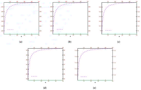
Figure 1. (a–e) The computational efficiency ratios of fractional simultaneous schemes with respect to each other for different fractional parameter values. (a) Computational efficiency ratio of $SF{M}^{{\sigma }_1}$ with respect to $SF{M}^{\sigma }$. (b) Computational efficiency ratio of $SF{M}^{{\sigma }_2}$ with respect to $SF{M}^{\sigma }$. (c) Computational efficiency ratio of $SF{M}^{{\sigma }_3}$ with respect to $SF{M}^{\sigma }$. (d) Computational efficiency ratio of $SF{M}^{{\sigma }_4}$ with respect to $SF{M}^{\sigma }$. (e) Computational efficiency ratio of $SF{M}^{\sigma }$ with respect to $SF{M}^{{\sigma }_1}$.

Here, ${\Lambda }_{11}=O\left(m\right)$, and SFM${}^{\sigma }$ is a simultaneous method for the fractional parameter value equals one.

5. Numerical Outcomes

To compare our recently developed simultaneous methods SFM${}^{{\sigma }_1}-$SFM${}^{{\sigma }_4}$ of order $3\varsigma +5$ to SFM${}^{\sigma }$, we look at a few numerical test examples in this section. With Maple 18’s 64 digits floating point arithmetic, all calculations were completed. The parallel computer algorithm was terminated based on the following conditions:  

$$e_i^{\left[\vartheta \right]}=\left|\left(r_i^{[\vartheta +1]}-r_i^{\left[\vartheta \right]}\right)\right|<\in ={10}^{-30},$$

where $e_i^{\left[\vartheta \right]}$ denotes the absolute error of consecutive iterations. In Table, 2-21, the numerical schemes for various fractional parameter values, i.e., 0.1, 0.3, 0.5, 0.8, 1.0, are represented by SFM${}^{{\sigma }_1}-$SFM${}^{{\sigma }_4}$, SFM${}^{\sigma }$ respectively, and B** denotes digits floating point arithmetic. In all tables, we use the following computer terminating criteria (Algorithm 1).

Algorithm 1 For the fractional numerical scheme SFMs${}^{\sigma }$

Engineering Applications

This section presents many problems in engineering whose solutions are approximated by our newly created parallel approaches SFM${}^{{\sigma }_1}-$SFM${}^{{\sigma }_4}$ and SFM${}^{\sigma }$.

Engineering Application 1: Emden–Fowler equation

The Emden–Fowler second-order nonlinear differential equation arises in various fields of physics and engineering, fluid dynamics, heat transfer, and astrophysics, in particular, to model the structure of self-gravitating, spherically symmetric objects, such as stars. The equation is named in honor of Ralph H. Fowler and Robert Emden, two German astrophysicists who made significant contributions to its formulation. The general form of the Emden–Fowler equation is given by [38,39]:

$$\left\{\begin{array}{c}\frac{d^{2}y}{d{r}^2}+g_1\left(r\right)\frac{dy}{dr}+g_2\left(r\right)y\left(r\right)+g\left(r\right)=y^n,\\ y\left(0\right)=0,y^{\prime }\left(0\right)=0.\end{array}\right.$$

(97)

Because of its nonlinearity, solving the Emden–Fowler equation is often difficult, and closed-form solutions exists only in specific cases. Choosing $n=2,$ $g_1\left(r\right)=\frac{5}{r},g_2\left(r\right)=\frac{3}{r^2},$ and $g\left(r\right)=r^4-15$ in (97), we obtain the following nonlinear initial value problem:

$$\left\{\begin{array}{c}\frac{d^{2}y}{d{r}^2}+\frac{5}{r}\frac{dy}{dr}+\frac{3}{r^2}y\left(r\right)+g\left(r\right)=y^2,\\ y\left(0\right)=0,y^{\prime }\left(0\right)=0.\end{array}\right.$$

(98)

Using the procedure described in [40], the numerical solution of (98) can be performed by solving the following polynomial:

$$f\left(r\right)=r^2-\frac{79}{28991745}{r}^{14}+\frac{1306}{57747104415}{r}^{18}.$$

(99)

The Caputo-type derivative of (99) is given as:

$$\left[{}_C{D}_{{\varsigma }_1}^{\varsigma }\right]f\left(r\right)=\frac{\Gamma \left(3\right)}{\Gamma (3-\varsigma )}{r}^{2-\varsigma }-\frac{79}{28991745}\frac{\Gamma \left(15\right)}{\Gamma (15-\varsigma )}{r}^{14-\varsigma }+\frac{1306}{57747104415}\left(\frac{\Gamma \left(19\right)}{\Gamma (19-\varsigma )}\right)r^{18-\varsigma }.$$

(100)

The exact solution of (99) up to four decimal places is:

$$\begin{array}{ccc}\hfill {\zeta }_1& =& -3.1792-0.2571i,{\zeta }_2=-3.1792+0.2575i,{\zeta }_3=-2.4135-1.4797i\hfill \\ \hfill {\zeta }_4& =& -2.4135+1.4797i,{\zeta }_5=-1.4797-2.4135i,{\zeta }_6=-1.4797+2.4135i\hfill \\ \hfill {\zeta }_7& =& -0.25758-3.1792i,{\zeta }_8=-0.2575+3.17923i,{\zeta }_{9,10}=0.0,\hfill \\ \hfill {\zeta }_{11}& =& 0.2575-3.17923i,{\zeta }_{12}=0.2575+3.1792i,{\zeta }_{13}=1.4797-2.4135i\hfill \\ \hfill {\zeta }_{14}& =& 1.4797+2.4135i,{\zeta }_{15}=2.41359-1.47975i,{\zeta }_{16}=2.4135+1.4797i\hfill \\ \hfill {\zeta }_{17}& =& 3.1792-0.25758i,{\zeta }_{18}=3.1792+0.2575i.\hfill \end{array}$$

In order to determine the global convergence behavior of the parallel scheme, we generate a random initial guess ranging from $r_{1*}^{\left[0\right]}$ to $r_{5*}^{\left[0\right]}$ using Matlab as explained in Appendix A Table A1. According to the results presented in Table 2, when an arbitrary starting value is used, SFM${}^{{\sigma }_1}-$SFM${}^{{\sigma }_4},$SFM${}^{\sigma }$ converges to exact zeros after 19, 17, 13, 10, and 10 iterations for fraction parameters 0.1, 0.3, 0.5, 0.8, and 1.0, respectively. The corresponding CPU times are 2.1254, 1.0874, 1.0078, 0.0784 and 0.0078 as shown in Table 3. The acceleration of the convergence rate of SFM${}^{{\sigma }_1}-$SFM${}^{{\sigma }_4},$SFM${}^{\sigma }$ as the fractional parameter value increases from 0.1 to 1.0 can be clearly seen in Table 4. Global convergence is demonstrated by the fact that the newly developed method converges to exact roots for randomly generated initial guess values.

Table 2. Experiments using random initial approximation for finding all polynomial roots simultaneously.

$\mathit{f}\left(\mathit{r}\right)={\mathit{r}}^2-\frac{79}{28991745}{\mathit{r}}^{14}+\frac{1306}{57747104415}{\mathit{r}}^{18}$
Ini-V	Number of Iterations
$r^{\left[0\right]}$	SFM${}^{{\sigma }_1}$	SFM${}^{{\sigma }_2}$	SFM${}^{{\sigma }_3}$	SFM${}^{{\sigma }_4}$	SFM${}^{\sigma }$
$r_{1*}^{\left[0\right]}$	19.0	17.0	13.0	10.0	10.0
$r_{2*}^{\left[0\right]}$	19.0	17.0	13.0	10.0	10.0
$r_{3*}^{\left[0\right]}$	19.0	17.0	13.0	10.0	10.0
$r_{4*}^{\left[0\right]}$	19.0	17.0	13.0	10.0	10.0
$r_{5*}^{\left[0\right]}$	19.0	17.0	13.0	10.0	10.0
Iteration are computed by using 64 D**

Table 3. CPU-Time using random initial approximation for finding all polynomial roots.

$\mathit{f}\left(\mathit{r}\right)={\mathit{r}}^2-\frac{79}{28991745}{\mathit{r}}^{14}+\frac{1306}{57747104415}{\mathit{r}}^{18}$
R-Initial	Computational CPU-Time in Seconds
$r^{\left[0\right]}$	SFM${}^{{\sigma }_1}$	SFM${}^{{\sigma }_2}$	SFM${}^{{\sigma }_3}$	SFM${}^{{\sigma }_4}$	SFM${}^{\sigma }$
$r_{1*}^{\left[0\right]}$	1.0124	1.0012	1.0014	0.0417	0.0045
$r_{2*}^{\left[0\right]}$	2.0125	1.0415	1.0045	0.0784	0.0048
$r_{3*}^{\left[0\right]}$	2.1254	1.0148	1.0047	0.0745	0.0078
$r_{4*}^{\left[0\right]}$	1.5241	1.0874	1.0078	0.0451	0.0071
$r_{5*}^{\left[0\right]}$	1.7451	1.0741	1.0078	0.0874	0.0069
Maximum CPU-Time is equal to 2.1254 using 64 D**

Table 4. Local computational order of convergence using random initial approximation.

$\mathit{f}\left(\mathit{r}\right)={\mathit{r}}^2-\frac{79}{28991745}{\mathit{r}}^{14}+\frac{1306}{57747104415}{\mathit{r}}^{18}$
Ini-V	Local Computational Order of Convergence
$r^{\left[0\right]}$	SFM${}^{{\sigma }_1}$	SFM${}^{{\sigma }_2}$	SFM${}^{{\sigma }_3}$	SFM${}^{{\sigma }_4}$	SFM${}^{\sigma }$
$r_{1*}^{\left[0\right]}$	6.0019	6.7215	7.7124	7.9115	7.9414
$r_{2*}^{\left[0\right]}$	7.0128	6.4515	7.4236	8.0365	7.5210
$r_{3*}^{\left[0\right]}$	4.9917	6.6454	7.0148	7.9914	7.8456
$r_{4*}^{\left[0\right]}$	5.8748	5.9874	7.5154	7.7214	8.0147
$r_{5*}^{\left[0\right]}$	6.1427	6.8748	7.3174	7.6148	7.4878
Maximum LCOC is equal to 8.0147 using 64 D**

Table 2 shows the number of iterations of the fractional simultaneous scheme SFM${}^{{\sigma }_1}-$SFM${}^{{\sigma }_4},$ SFM${}^{\sigma }$ for different choices of the random initial vector given in Appendix A, Table A1. Table 2 clearly shows that the number of iterations decreased as the fractional parameter values increased from 0.1 to 1.0.

Table 5 shows the maximum error (Max-Err) computed by the fractional simultaneous scheme SFM${}^{{\sigma }_1}-$SFM${}^{{\sigma }_4},$ SFM${}^{\sigma }$ for different selections of the random initial vector given in Appendix A Table A1 to approximate all roots of the polynomial equations used in application 1. Table 5 clearly demonstrates that as the fractional parameter values increased from 0.1 to 1.0, the accuracy computed by the simultaneous scheme increased significantly (Figure 2).

Table 5. Maximum error using random initial approximation for finding all polynomial roots.

$\mathit{f}\left(\mathit{r}\right)=-2949.604{\mathit{r}}^4+14748.02{\mathit{r}}^3-62295.63648{\mathit{r}}^2+2.229900624\times {10}^5\mathit{r}-2.675880749\times {10}^5$
R-Initial	Maximum Error
$r^{\left[0\right]}$	SFM${}^{{\sigma }_1}$	SFM${}^{{\sigma }_2}$	SFM${}^{{\sigma }_3}$	SFM${}^{{\sigma }_4}$	SFM${}^{\sigma }$
$r_{1*}^{\left[0\right]}$	$3.1\times {10}^{-15}$	$0.1\times {10}^{-18}$	$6.3\times {10}^{-20}$	$9.5\times {10}^{-22}$	$0.2\times {10}^{-29}$
$r_{2*}^{\left[0\right]}$	$0.01\times {10}^{-15}$	$1.2\times {10}^{-18}$	$6.5\times {10}^{-24}$	$8.8\times {10}^{-27}$	$3.5\times {10}^{-20}$
$r_{3*}^{\left[0\right]}$	$0.1\times {10}^{-14}$	$0.1\times {10}^{-18}$	$0.1\times {10}^{-22}$	$3.8\times {10}^{-25}$	$1.5\times {10}^{-25}$
$r_{4*}^{\left[0\right]}$	$0.4\times {10}^{-13}$	$9.5\times {10}^{-18}$	$9.0\times {10}^{-21}$	$3.2\times {10}^{-20}$	$1.2\times {10}^{-25}$
$r_{5*}^{\left[0\right]}$	$7.7\times {10}^{-15}$	$7.8\times {10}^{-18}$	$3.9\times {10}^{-21}$	$0.2\times {10}^{-31}$	$0.5\times {10}^{-31}$
Residual errors are equal to 10${}^{-30}$ using 64 D**

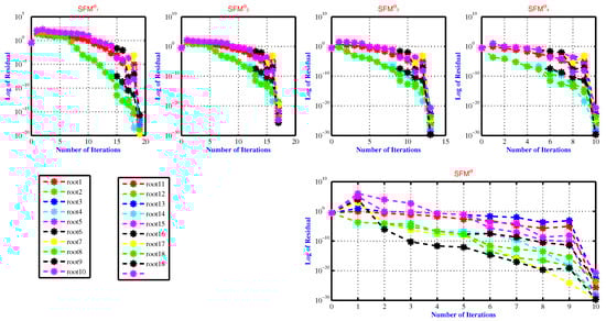
Figure 2. Residual error of the SFM${}^{\sigma }$ for approximating all polynomial equation roots used in engineering application 1 for various fractional parameter values, namely $\varsigma =0.1,0.3,0.7,0.8,1.0$.

Table 4 shows the approximate local computational order of convergence. The approximate local computational order of convergence increases as the fractional parameter values increase from 0.1 to 1.0.

Table 3 shows the computational CPU time in seconds to approximate all roots of the polynomial equation used in application 1 employing the fractional simultaneous scheme.

The rate of convergence increases as the initial guess values are chosen to be sufficiently close to the exact root of (99) as:

$$\begin{array}{ccc}\hfill r_1^{\left[0\right]}& =& -3.1-0.2i,r_2^{\left[0\right]}=-3.1+0.2i,r_3^{\left[0\right]}=-2.4-1.4i\hfill \\ \hfill r_4^{\left[0\right]}& =& -2.4+1.4i,r_5^{\left[0\right]}=-1.4-2.4i,r_6^{\left[0\right]}=-1.4+2.4i\hfill \\ \hfill r_7^{\left[0\right]}& =& -0.2-3.1i,r_8^{\left[0\right]}=-0.2+3.1i,r_9^{\left[0\right]}=0.02,r_{10}^{\left[0\right]}=0.01,\hfill \\ \hfill r_{11}^{\left[0\right]}& =& 0.2-3.1i,r_{12}^{\left[0\right]}=0.2+3.1i,r_{13}^{\left[0\right]}=1.4-2.4i\hfill \\ \hfill r_{14}^{\left[0\right]}& =& 1.4+2.4i,r_{15}^{\left[0\right]}=2.4-1.4i,r_{16}^{\left[0\right]}=2.4+1.4i\hfill \\ \hfill r_{17}^{\left[0\right]}& =& 3.1-0.2i,r_{18}^{\left[0\right]}=3.1+0.2i.\hfill \end{array}$$

If we start with initial guessed values that are close to the exact root, Table 6 demonstrates that the fractional simultaneous scheme’s accuracy and convergence order improve. As the fractional parameter value was increased from 0.1 to 1.0, the residual error calculated using numerical methods also increased.

Table 6. Computation of all polynomial equation roots.

Methods	SFM${}^{{\mathit{\sigma }}_1}$	SFM${}^{{\mathit{\sigma }}_2}$	SFM${}^{{\mathit{\sigma }}_3}$	SFM${}^{{\mathit{\sigma }}_4}$	SFM${}^{\mathit{\sigma }}$
Error it	$\vartheta =09$	$\vartheta =09$	$\vartheta =07$	$\vartheta =06$	$\vartheta =06$
CPU	0.0141	0.016	0.054	0.067	0.065
$e_1^{\left[\vartheta \right]}$	$2.1\times {10}^{-3}$	$0.7\times {10}^{-3}$	$0.3\times {10}^{-12}$	$0.7\times {10}^{-32}$	$0.3\times {10}^{-42}$
$e_2^{\left[\vartheta \right]}$	$5.2\times {10}^{-2}$	$2.6\times {10}^{-4}$	$9.1\times {10}^{-16}$	$2.1\times {10}^{-26}$	$2.8\times {10}^{-64}$
$e_3^{\left[\vartheta \right]}$	$2.1\times {10}^{-2}$	$3.2\times {10}^{-3}$	$3.2\times {10}^{-16}$	$3.2\times {10}^{-36}$	$3.5\times {10}^{-46}$
$e_4^{\left[\vartheta \right]}$	$3.1\times {10}^{-2}$	$4.1\times {10}^{-6}$	$4.1\times {10}^{-16}$	$4.1\times {10}^{-26}$	$4.1\times {10}^{-46}$
$e_5^{\left[\vartheta \right]}$	$2.1\times {10}^{-3}$	$0.7\times {10}^{-3}$	$0.3\times {10}^{-12}$	$0.7\times {10}^{-32}$	$0.3\times {10}^{-42}$
$e_6^{\left[\vartheta \right]}$	$2.0\times {10}^{-3}$	$0.7\times {10}^{-3}$	$0.3\times {10}^{-12}$	$0.7\times {10}^{-32}$	$0.3\times {10}^{-42}$
$e_7^{\left[\vartheta \right]}$	$0.2\times {10}^{-2}$	$0.1\times {10}^{-4}$	$9.1\times {10}^{-16}$	$4.1\times {10}^{-26}$	$2.7\times {10}^{-43}$
$e_8^{\left[\vartheta \right]}$	$5.1\times {10}^{-2}$	$1.2\times {10}^{-5}$	$1.1\times {10}^{-14}$	$0.2\times {10}^{-31}$	$3.0\times {10}^{-42}$
$e_9^{\left[\vartheta \right]}$	$0.1\times {10}^{-3}$	$0.6\times {10}^{-6}$	$0.1\times {10}^{-15}$	$4.1\times {10}^{-26}$	$6.1\times {10}^{-36}$
$e_{10}^{\left[\vartheta \right]}$	$5.2\times {10}^{-2}$	$2.9\times {10}^{-4}$	$9.1\times {10}^{-16}$	$4.1\times {10}^{-26}$	$2.7\times {10}^{-43}$
$e_{11}^{\left[\vartheta \right]}$	$0.1\times {10}^{-1}$	$1.2\times {10}^{-5}$	$1.1\times {10}^{-14}$	$0.2\times {10}^{-31}$	$3.0\times {10}^{-42}$
$e_{12}^{\left[\vartheta \right]}$	$0.2\times {10}^{-1}$	$3.6\times {10}^{-2}$	$9.8\times {10}^{-16}$	$8.1\times {10}^{-26}$	$2.6\times {10}^{-42}$
$e_{13}^{\left[\vartheta \right]}$	$2.8\times {10}^{-2}$	$7.2\times {10}^{-3}$	$3.2\times {10}^{-16}$	$0.7\times {10}^{-36}$	$3.3\times {10}^{-45}$
$e_{14}^{\left[\vartheta \right]}$	$1.1\times {10}^{-2}$	$1.2\times {10}^{-5}$	$4.1\times {10}^{-14}$	$4.2\times {10}^{-31}$	$3.0\times {10}^{-42}$
$e_{15}^{\left[\vartheta \right]}$	$0.1\times {10}^{-3}$	$0.7\times {10}^{-3}$	$7.3\times {10}^{-12}$	$0.7\times {10}^{-32}$	$1.3\times {10}^{-41}$
$e_{16}^{\left[\vartheta \right]}$	$0.2\times {10}^{-2}$	$3.6\times {10}^{-4}$	$9.8\times {10}^{-16}$	$8.1\times {10}^{-26}$	$2.6\times {10}^{-42}$
$e_{17}^{\left[\vartheta \right]}$	$2.8\times {10}^{-2}$	$7.2\times {10}^{-3}$	$3.2\times {10}^{-16}$	$0.0\times {10}^{-36}$	$3.3\times {10}^{-45}$
$e_{18}^{\left[\vartheta \right]}$	$8.1\times {10}^{-2}$	$0.1\times {10}^{-6}$	$4.1\times {10}^{-16}$	$0.1\times {10}^{-26}$	$4.1\times {10}^{-46}$
${\rho }_i^{[\vartheta -1]}$	2.1212	2.2312	2.0451	2.5112	3.14212

Engineering Application 2: Under Conservative Force—Mass Spring System

Let us now examine an external force acting on a vibrating mass on a spring. A driving force that causes the spring support to oscillate vertically, for instance, could be represented by $f\left(r\right)$. If the mechanical system is conservative, the following nonlinear equation arises [41,42]:

$$\left\{\begin{array}{c}{f}^{″}\left(r\right)+{\left(f^{\prime }\left(r\right)\right)}^2+32-160r=0,\\ f\left(0\right)=0,f^{\prime }\left(0\right)=0.\end{array}\right.$$

(101)

Using the method described in [40], the following polynomial is used to simulate (101) as:

$$\begin{array}{ccc}\hfill f\left(r\right)& =& -\frac{43359567872}{189}{r}^{10}+\frac{425993216}{405}{r}^9-\frac{278592512}{63}{r}^8+\hfill \\ & & \frac{1024000}{63}{r}^7-\frac{4096384}{45}{r}^6+256r^5\hfill \\ & & -\frac{6400}{3}{r}^4+\frac{16}{3}{r}^3-80r^2.\hfill \end{array}$$

(102)

The Caputo-type derivative of (102) is given as:

$$\begin{array}{ccc}\hfill \left[{}_C{D}_{{\varsigma }_1}^{\varsigma }\right]f\left(r\right)& =& -\frac{43359567872}{189}\frac{\Gamma \left(11\right)}{\Gamma (11-\varsigma )}{r}^{10-\varsigma }+\frac{425993216}{405}\frac{\Gamma \left(10\right)}{\Gamma (10-\varsigma )}{r}^{9-\varsigma }-\hfill \\ & & \frac{278592512}{63}\frac{\Gamma \left(9\right)}{\Gamma (9-\varsigma )}{r}^{8-\varsigma }+\frac{1024000}{63}\frac{\Gamma \left(8\right)}{\Gamma (8-\varsigma )}{r}^{7-\varsigma }-\hfill \\ & & \frac{4096384}{45}\frac{\Gamma \left(7\right)}{\Gamma (7-\varsigma )}{r}^{6-\varsigma }+256\frac{\Gamma \left(6\right)}{\Gamma (6-\varsigma )}{r}^{5-\varsigma }-\hfill \\ & & \frac{6400}{3}\frac{\Gamma \left(5\right)}{\Gamma (5-\varsigma )}{r}^{4-\varsigma }+\frac{16}{3}\frac{\Gamma \left(4\right)}{\Gamma (4-\varsigma )}{r}^{3-\varsigma }-80\frac{\Gamma \left(3\right)}{\Gamma (3-\varsigma )}{r}^{2-\varsigma }\hfill \end{array}$$

(103)

The exact solution up to four decimal places is written as:

$$\begin{array}{ccc}\hfill {\zeta }_1& =& -0.12909-0.0824i,{\zeta }_2=-0.1290+0.0824i,{\zeta }_3=-0.0513-0.1495i,\hfill \\ \hfill {\zeta }_4& =& -0.0513+0.1495i,{\zeta }_{5,6}=0.0,{\zeta }_7=0.0525-0.1493i,{\zeta }_8=0.0525+0.1493i,\hfill \\ \hfill {\zeta }_9& =& 0.1301-0.0822i,{\zeta }_{10}=0.13010+0.0822i.\hfill \end{array}$$

To determine the global convergence component of the parallel scheme, use Matlab to generate a random initial guess value ranging from $r_{1*}^{\left[0\right]}-r_{5*}^{\left[0\right]}$ as specified in Appendix A Table A2. With an arbitrary starting value, SFM${}^{{\sigma }_1}-$SFM${}^{{\sigma }_4},$ SFM${}^{\sigma }$ converges to exact zeros after 19, 16, 14, 10 and 10 iterations as indicated in Table 7 for fraction parameters values 0.1, 0.3, 0.5, 0.8, and 1.0, respectively. As described in Table 8, the corresponding CPU times are 3.1254, 1.0729, 1.0137, 0.0881 and 0.0141, respectively. Table 9 clearly illustrates how the rate of convergence of SFM${}^{{\sigma }_1}-$SFM${}^{{\sigma }_4},$SFM${}^{\sigma }$ accelerates as the value of the fractional parameter increases from 0.1 to 1.0. The newly developed method converges to exact roots for randomly generated initial guess values, demonstrating its global convergence.

Table 7. Iteration numbers using random initial approximation for finding all polynomial roots.

$\mathit{f}\left(\mathit{r}\right)=-\frac{43359567872}{189}{\mathit{r}}^{10}+\frac{425993216}{405}{\mathit{r}}^9-\frac{278592512}{63}{\mathit{r}}^8+$
$\frac{\mathbf{1024000}}{\mathbf{63}}{\mathit{r}}^{\mathbf{7}}-\frac{\mathbf{4096384}}{\mathbf{45}}{\mathit{r}}^{\mathbf{6}}+\mathbf{256}{\mathit{r}}^{\mathbf{5}}-\frac{\mathbf{6400}}{\mathbf{3}}{\mathit{r}}^{\mathbf{4}}+$
$\frac{\mathbf{16}}{\mathbf{3}}{\mathit{r}}^{\mathbf{3}}-\mathbf{80}{\mathit{r}}^{\mathbf{2}}.$
Ini-V	Number of Iterations
$r^{\left[0\right]}$	SFM${}^{{\sigma }_1}$	SFM${}^{{\sigma }_2}$	SFM${}^{{\sigma }_3}$	SFM${}^{{\sigma }_4}$	SFM${}^{\sigma }$
$r_{1*}^{\left[0\right]}$	19.0	16.0	14.0	10.0	10.0
$r_{2*}^{\left[0\right]}$	19.0	16.0	14.0	10.0	10.0
$r_{3*}^{\left[0\right]}$	19.0	16.0	14.0	10.0	10.0
$r_{4*}^{\left[0\right]}$	19.0	16.0	14.0	10.0	10.0
$r_{5*}^{\left[0\right]}$	19.0	16.0	14.0	10.0	10.0
Residual errors are equal to 10${}^{-30}$ using 64 D**

Table 8. CPU-Time using random initial approximation for finding all polynomial roots.

$\mathit{f}\left(\mathit{r}\right)=-\frac{43359567872}{189}{\mathit{r}}^{10}+\frac{425993216}{405}{\mathit{r}}^9-\frac{278592512}{63}{\mathit{r}}^8+$
$\frac{\mathbf{1024000}}{\mathbf{63}}{\mathit{r}}^{\mathbf{7}}-\frac{\mathbf{4096384}}{\mathbf{45}}{\mathit{r}}^{\mathbf{6}}+\mathbf{256}{\mathit{r}}^{\mathbf{5}}-\frac{\mathbf{6400}}{\mathbf{3}}{\mathit{r}}^{\mathbf{4}}+$
$\frac{\mathbf{16}}{\mathbf{3}}{\mathit{r}}^{\mathbf{3}}-\mathbf{80}{\mathit{r}}^{\mathbf{2}}.$
R-Initial	Computational CPU-Time in Seconds
$r^{\left[0\right]}$	SFM${}^{{\sigma }_1}$	SFM${}^{{\sigma }_2}$	SFM${}^{{\sigma }_3}$	SFM${}^{{\sigma }_4}$	SFM${}^{\sigma }$
$r_{1*}^{\left[0\right]}$	3.0114	1.0012	0.0015	0.0417	0.0031
$r_{2*}^{\left[0\right]}$	2.1105	1.0317	1.0080	0.0881	0.0141
$r_{3*}^{\left[0\right]}$	3.1254	1.0159	1.0137	0.0765	0.0039
$r_{4*}^{\left[0\right]}$	1.4201	1.0678	1.0061	0.0430	0.0067
$r_{5*}^{\left[0\right]}$	1.7465	1.0729	1.0070	0.09143	0.0073
Residual errors are equal to 10${}^{-30}$ using 64 D**

Table 9. Maximum error using random initial approximation for finding all polynomial roots.

$\mathit{f}\left(\mathit{r}\right)=-\frac{43359567872}{189}{\mathit{r}}^{10}+\frac{425993216}{405}{\mathit{r}}^9-\frac{278592512}{63}{\mathit{r}}^8+\frac{1024000}{63}{\mathit{r}}^7-\frac{4096384}{45}{\mathit{r}}^6+256{\mathit{r}}^5-\frac{6400}{3}{\mathit{r}}^4+\frac{16}{3}{\mathit{r}}^3-80{\mathit{r}}^2.$
R-Initial	Maximum Error
$r^{\left[0\right]}$	SFM${}^{{\sigma }_1}$	SFM${}^{{\sigma }_2}$	SFM${}^{{\sigma }_3}$	SFM${}^{{\sigma }_4}$	SFM${}^{\sigma }$
$r_{1*}^{\left[0\right]}$	$0.1\times {10}^{-16}$	$1.1\times {10}^{-18}$	$6.3\times {10}^{-20}$	$4.5\times {10}^{-23}$	$6.1\times {10}^{-25}$
$r_{2*}^{\left[0\right]}$	$2.1\times {10}^{-16}$	$6.2\times {10}^{-19}$	$1.5\times {10}^{-24}$	$7.8\times {10}^{-26}$	$3.0\times {10}^{-26}$
$r_{3*}^{\left[0\right]}$	$0.1\times {10}^{-15}$	$6.1\times {10}^{-18}$	$0.4\times {10}^{-24}$	$7.8\times {10}^{-26}$	$2.5\times {10}^{-27}$
$r_{4*}^{\left[0\right]}$	$3.4\times {10}^{-14}$	$6.5\times {10}^{-18}$	$0.1\times {10}^{-20}$	$3.2\times {10}^{-28}$	$6.2\times {10}^{-25}$
$r_{5*}^{\left[0\right]}$	$9.7\times {10}^{-17}$	$1.8\times {10}^{-19}$	$3.2\times {10}^{-21}$	$9.2\times {10}^{-33}$	$3.5\times {10}^{-32}$
Residual errors are equal to 10${}^{-30}$ using 64 D**

Table 7 shows the number of iterations of fractional simultaneous scheme SFM${}^{{\sigma }_1}-$SFM${}^{{\sigma }_4},$ SFM${}^{\sigma }$ for different random initial vectors given in Appendix A Table A2. Table 7 clearly shows that the number of iterations decreased as the fractional parameter values increased from 0.1 to 1.0.

Table 9 shows the maximum error (Max-Err) computed by fractional simultaneous scheme SFM${}^{{\sigma }_1}-$SFM${}^{{\sigma }_4},$ SFM${}^{\sigma }$ for different random initial vectors given in Appendix A Table A2 to approximate all the roots of polynomial equations used in application 2. Table 9 clearly demonstrates that as the fractional parameter values increased from 0.1 to 1.0, the accuracy computed by simultaneous scheme increased significantly (Figure 3).

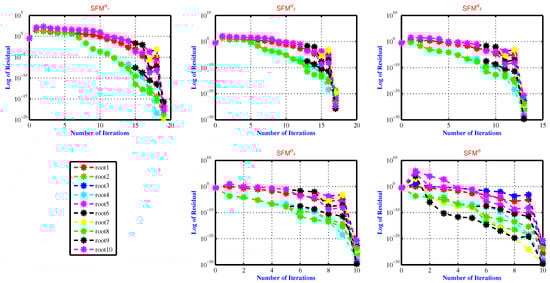
Figure 3. The residual error of SFM${}^{\sigma }$ for approximating all polynomial equation roots used in engineering application 2 for various fractional parameter values, namely $\varsigma =0.1,0.3,0.7,0.8,1.0$.

The approximate local computational order of convergence is shown in Table 10. From 0.1 to 1.0, as the fractional parameter values increase, the approximate local computational order of convergence increases.

Table 10. Local computational order of convergence using random initial approximation.

$\mathit{f}\left(\mathit{r}\right)=-\frac{43359567872}{189}{\mathit{r}}^{10}+\frac{425993216}{405}{\mathit{r}}^9-\frac{278592512}{63}{\mathit{r}}^8+$
$\frac{\mathbf{1024000}}{\mathbf{63}}{\mathit{r}}^{\mathbf{7}}-\frac{\mathbf{4096384}}{\mathbf{45}}{\mathit{r}}^{\mathbf{6}}+\mathbf{256}{\mathit{r}}^{\mathbf{5}}-\frac{\mathbf{6400}}{\mathbf{3}}{\mathit{r}}^{\mathbf{4}}+$
$\frac{\mathbf{16}}{\mathbf{3}}{\mathit{r}}^{\mathbf{3}}-\mathbf{80}{\mathit{r}}^{\mathbf{2}}.$
Ini-V	Local Computational Order of Conergence
$r^{\left[0\right]}$	SFM${}^{{\sigma }_1}$	SFM${}^{{\sigma }_2}$	SFM${}^{{\sigma }_3}$	SFM${}^{{\sigma }_4}$	SFM${}^{\sigma }$
$r_{1*}^{\left[0\right]}$	5.0119	6.7005	7.7354	7.9195	7.9654
$r_{2*}^{\left[0\right]}$	7.0128	6.4515	7.4236	7.4365	8.1210
$r_{3*}^{\left[0\right]}$	4.9917	6.6454	7.0148	7.9914	7.8456
$r_{4*}^{\left[0\right]}$	5.1708	4.9104	7.5154	7.7114	8.0101
$r_{5*}^{\left[0\right]}$	5.1127	5.8018	7.0074	7.0048	7.9018
Residual errors are equal to 10${}^{-30}$ using 64 D**

According to the fractional simultaneous scheme, Table 10 displays the local computational order of convergence needed for the approximation of all roots of the polynomial equation used in application 2. Convergence rates increase as the following initial estimations are sufficiently adjusted to the exact roots of the engineering application 2:

$$\begin{array}{ccc}\hfill r_1^{\left[0\right]}& =& -0.1-0.01i,r_2^{\left[0\right]}=-0.1+0.01i,r_3^{\left[0\right]}=-0.01-0.1i,\hfill \\ \hfill r_4^{\left[0\right]}& =& -0.01+0.1i,r_5^{\left[0\right]}=0.01,r_6^{\left[0\right]}-0.1,r_7^{\left[0\right]}=0.05-0.14i,\hfill \\ \hfill r_8^{\left[0\right]}& =& 0.05+0.14i,r_9^{\left[0\right]}=0.1-0.08i,r_{10}^{\left[0\right]}=0.1+0.08i.\hfill \end{array}$$

are chosen as initial guessed values.

Table 11 shows that the convergence order and accuracy of the fractional simultaneous scheme are increased if we take the initial guessed values close to the exact root. The residual error computed by numerical methods also increased as we increased the fractional parameter value from 0.1 to 1.0.

Table 11. Determination of all polynomial equation roots.

Methods	SFM${}^{{\mathit{\sigma }}_1}$	SFM${}^{{\mathit{\sigma }}_2}$	SFM${}^{{\mathit{\sigma }}_3}$	SFM${}^{{\mathit{\sigma }}_4}$	SFM${}^{\mathit{\sigma }}$
Error it	$\vartheta =09$	$\vartheta =09$	$\vartheta =08$	$\vartheta =08$	$\vartheta =05$
CPU	0.0141	0.016	0.054	0.067	0.065
$e_1^{\left[\vartheta \right]}$	$0.2\times {10}^{-3}$	$1.7\times {10}^{-4}$	$1.3\times {10}^{-11}$	$5.7\times {10}^{-33}$	$0.3\times {10}^{-42}$
$e_2^{\left[\vartheta \right]}$	$7.2\times {10}^{-2}$	$2.8\times {10}^{-5}$	$9.9\times {10}^{-17}$	$5.5\times {10}^{-27}$	$2.8\times {10}^{-46}$
$e_3^{\left[\vartheta \right]}$	$2.5\times {10}^{-3}$	$3.2\times {10}^{-3}$	$3.2\times {10}^{-16}$	$1.2\times {10}^{-36}$	$3.0\times {10}^{-47}$
$e_4^{\left[\vartheta \right]}$	$3.1\times {10}^{-2}$	$9.9\times {10}^{-7}$	$4.8\times {10}^{-16}$	$4.9\times {10}^{-23}$	$4.1\times {10}^{-46}$
$e_5^{\left[\vartheta \right]}$	$7.7\times {10}^{-3}$	$6.7\times {10}^{-6}$	$6.5\times {10}^{-16}$	$6.5\times {10}^{-26}$	$6.5\times {10}^{-46}$
$e_6^{\left[\vartheta \right]}$	$2.5\times {10}^{-2}$	$4.3\times {10}^{-7}$	$4.8\times {10}^{-17}$	$4.0\times {10}^{-27}$	$4.0\times {10}^{-47}$
$e_7^{\left[\vartheta \right]}$	$1.6\times {10}^{-2}$	$3.0\times {10}^{-6}$	$3.0\times {10}^{-16}$	$7.7\times {10}^{-36}$	$3.0\times {10}^{-46}$
$e_8^{\left[\vartheta \right]}$	$7.4\times {10}^{-3}$	$4.4\times {10}^{-7}$	$2.9\times {10}^{-15}$	$2.9\times {10}^{-40}$	$2.4\times {10}^{-46}$
$e_9^{\left[\vartheta \right]}$	$3.0\times {10}^{-4}$	$2.8\times {10}^{-6}$	$2.0\times {10}^{-16}$	$2.7\times {10}^{-35}$	$1.1\times {10}^{-49}$
$e_{10}^{\left[\vartheta \right]}$	$3.5\times {10}^{-2}$	$2.1\times {10}^{-7}$	$4.5\times {10}^{-16}$	$2.0\times {10}^{-39}$	$2.7\times {10}^{-41}$
${\rho }_i^{[\vartheta -1]}$	2.1012	2.2452	2.0491	3.5112	3.18742

Engineering Application 3: Series Circuit Analogue

Consider a flexible spring that is stretched vertically from a rigid support and has a mass m attached to its free end. Naturally, the mass will determine how much the spring elongates or stretches; different weight masses will result in different ways that the spring will stretch. Hooke’s law states that the spring itself generates a restoring force F that is opposed to the direction of elongation and proportional to the amount of elongation s. In short, a proportionality constant is defined as $F=ks$, where k is the spring constant. In an undamped spring/mass system, the differential equation represents $F\left(x\right)$, which is mathematically modeled as [40,42]:

$$\left\{\begin{array}{c}\frac{d^{2}y}{d{r}^2}+y^3=0,\\ y\left(0\right)=1,y^{\prime }\left(0\right)=1.\end{array}\right.$$

(104)

Using the method described in [40], the following polynomial is used to simulate (104) as:

$$f\left(r\right)=-0.5r^3-0.5r^2+r+1.$$

(105)

The Caputo-type derivative of (105) is given as:

$$\left[{}_C{D}_{{\varsigma }_1}^{\varsigma }\right]f\left(r\right)=-0.5\frac{\Gamma \left(4\right)}{\Gamma (4-\varsigma )}{r}^{3-\varsigma }-0.5\frac{\Gamma \left(3\right)}{\Gamma (3-\varsigma )}{r}^{2-\varsigma }+\frac{\Gamma \left(2\right)}{\Gamma (2-\varsigma )}{r}^{1-\varsigma }+\frac{1}{\Gamma (1-\varsigma )}{r}^{-\varsigma },$$

(106)

The exact solution of (105) up to the decimal places is written as follows:

$${\zeta }_1=-1,{\zeta }_2=1.414213562,{\zeta }_3=-1.414213562.$$

To determine the global convergence component of the parallel scheme, use Matlab to generate a random initial guess value ranging from $r_{1*}^{\left[0\right]}-r_{5*}^{\left[0\right]}$ as specified in Appendix A Table A3. With an arbitrary starting value, SFM${}^{{\sigma }_1}-$SFM${}^{{\sigma }_4},$ SFM${}^{\sigma }$ converges to exact zeros after 19, 16, 13, 8, and 8 iterations as indicated in Table 12 for various fractional parameters, i.e., 0.1, 0.3, 0.5, 0.8, and 1.0. As described in Table 13, the corresponding CPU times are 3.1364, 1.0701, 1.0078, 0.0874 and 0.0975, respectively. Table 14 clearly illustrates how the rate of convergence of SFM${}^{{\sigma }_1}-$SFM${}^{{\sigma }_4},$ SFM${}^{\sigma }$ accelerates as the value of the fractional parameter increases from 0.1 to 1.0. The newly developed method converges to exact roots for randomly generated initial guess values, demonstrating its global convergence.

Table 12. Using random initial approximation for finding all polynomial roots simultaneously.

$\mathit{f}\left(\mathit{r}\right)=-0.5{\mathit{r}}^3-0.5{\mathit{r}}^2+\mathit{r}+1$
Ini-V	Number of Iterations
$r^{\left[0\right]}$	SFM${}^{{\sigma }_1}$	SFM${}^{{\sigma }_2}$	SFM${}^{{\sigma }_3}$	SFM${}^{{\sigma }_4}$	SFM${}^{\sigma }$
$r_{1*}^{\left[0\right]}$	19.0	16.0	13.0	8.0	8.0
$r_{2*}^{\left[0\right]}$	19.0	16.0	13.0	8.0	8.0
$r_{3*}^{\left[0\right]}$	19.0	16.0	13.0	8.0	8.0
$r_{4*}^{\left[0\right]}$	19.0	16.0	13.0	8.0	8.0
$r_{5*}^{\left[0\right]}$	19.0	16.0	13.0	8.0	8.0
Residual errors are equal to 10${}^{-30}$ using 64 D**

Table 13. CPU-Time using random initial values for finding all polynomial roots.

$\mathit{f}\left(\mathit{r}\right)=-0.5{\mathit{r}}^3-0.5{\mathit{r}}^2+\mathit{r}+1$
Ini-V	Computational CPU-Time in Seconds
$r^{\left[0\right]}$	SFM${}^{{\sigma }_1}$	SFM${}^{{\sigma }_2}$	SFM${}^{{\sigma }_3}$	SFM${}^{{\sigma }_4}$	SFM${}^{\sigma }$
$r_{1*}^{\left[0\right]}$	0.0159	0.0491	1.4514	0.0319	0.0455
$r_{2*}^{\left[0\right]}$	2.0136	1.0464	1.0045	0.0694	0.0107
$r_{3*}^{\left[0\right]}$	3.1364	1.0139	1.0047	0.0646	0.0059
$r_{4*}^{\left[0\right]}$	1.5209	0.0874	1.0078	0.0456	0.0975
$r_{5*}^{\left[0\right]}$	1.7451	1.0701	1.0038	0.0874	0.0048
Maximum CPU-Time is equale to 2.1254 using 64 D**

Table 14. Maximum error using random initial approximation for finding all polynomial roots.

$\mathit{f}\left(\mathit{r}\right)=-0.5{\mathit{r}}^3-0.5{\mathit{r}}^2+\mathit{r}+1$
R-Initial	Maximum Error
$r^{\left[0\right]}$	SFM${}^{{\sigma }_1}$	SFM${}^{{\sigma }_2}$	SFM${}^{{\sigma }_3}$	SFM${}^{{\sigma }_4}$	SFM${}^{\sigma }$
$r_{1*}^{\left[0\right]}$	$3.2\times {10}^{-19}$	$9.1\times {10}^{-17}$	$0.3\times {10}^{-21}$	$9.5\times {10}^{-22}$	$9.1\times {10}^{-23}$
$r_{2*}^{\left[0\right]}$	$2.4\times {10}^{-16}$	$1.2\times {10}^{-17}$	$6.1\times {10}^{-25}$	$8.1\times {10}^{-29}$	$3.5\times {10}^{-27}$
$r_{3*}^{\left[0\right]}$	$0.1\times {10}^{-14}$	$0.5\times {10}^{-19}$	$0.4\times {10}^{-23}$	$0.8\times {10}^{-20}$	$9.5\times {10}^{-28}$
$r_{4*}^{\left[0\right]}$	$6.4\times {10}^{-15}$	$6.5\times {10}^{-18}$	$0.1\times {10}^{-20}$	$3.2\times {10}^{-28}$	$6.2\times {10}^{-25}$
$r_{5*}^{\left[0\right]}$	$7.7\times {10}^{-15}$	$7.8\times {10}^{-18}$	$7.2\times {10}^{-23}$	$6.6\times {10}^{-36}$	$6.7\times {10}^{-31}$
Residual errors are equal to 10${}^{-30}$ using 64 D**

Table 12 shows the number of iterations of fractional simultaneous scheme SFM${}^{{\sigma }_1}-$SFM${}^{{\sigma }_4},$ SFM${}^{\sigma }$ for different random initial vectors given in Appendix A Table A3. Table 12 clearly shows that the number of iterations decreased as the fractional parameter values increased from 0.1 to 1.0.

Table 14 shows the maximum error (Max-Err) computed by fractional simultaneous scheme SFM${}^{{\sigma }_1}-$SFM${}^{{\sigma }_3},$ SFM${}^{\sigma }$ for different random initial vectors given in Appendix A Table A3 to approximate all roots of the polynomial equations used in application 3. Table 14 clearly demonstrates that as the fractional parameter values increased from 0.1 to 1.0, the accuracy computed by simultaneous scheme increased significantly (Figure 4).

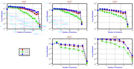
Figure 4. The residual error of the SFM${}^{\sigma }$ for approximating all polynomial equation roots used in engineering application 3 for various fractional parameter values, namely $\varsigma =0.1,0.3,0.7,0.8,1.0$.

The approximate local computational order of convergence is shown in Table 15. As the fractional parameter values increase from 0.1 to 1.0, the approximate local computational order of convergence increases.

Table 15. Local computational order of convergence using random initial approximation.

$\mathit{f}\left(\mathit{r}\right)=-0.5{\mathit{r}}^3-0.5{\mathit{r}}^2+\mathit{r}+1$
Ini-V	Local Computational Order of Convergence
$r^{\left[0\right]}$	SFM${}^{{\sigma }_1}$	SFM${}^{{\sigma }_2}$	SFM${}^{{\sigma }_3}$	SFM${}^{{\sigma }_4}$	SFM${}^{\sigma }$
$r_{1*}^{\left[0\right]}$	5.0429	6.4013	7.1234	7.9011	7.9012
$r_{2*}^{\left[0\right]}$	7.0128	6.4515	7.4416	8.1301	7.9210
$r_{3*}^{\left[0\right]}$	5.5927	6.6114	6.9141	7.0914	8.8151
$r_{4*}^{\left[0\right]}$	5.4501	5.9174	7.5124	7.7014	8.0140
$r_{5*}^{\left[0\right]}$	5.1121	6.5701	7.1104	7.8108	8.0038
Residual errors are equal to 10${}^{-30}$ using 64 D**

Table 13 displays the computational CPU time in seconds required to approximate all roots of the polynomial equation used in application 3 using the fractional simultaneous scheme.

Convergence rates increase as the following initial estimations are sufficiently adjusted to the exact root of engineering application 3:

$$r_1^{\left[0\right]}=-0.1,r_2^{\left[0\right]}=1.4,r_3^{\left[0\right]}=-1.4,$$

are chosen as the initial guessed values.

Table 16 shows how the convergence order and accuracy of the fractional simultaneous scheme increase when we use initial guessed values close to the exact root. The residual error computed by numerical schemes increased as we increased the fractional parameter value from 0.1 to 1.0.

Table 16. Determination of all polynomial equation roots.

Methods	SFM${}^{{\mathit{\sigma }}_1}$	SFM${}^{{\mathit{\sigma }}_2}$	SFM${}^{{\mathit{\sigma }}_3}$	SFM${}^{{\mathit{\sigma }}_4}$	SFM${}^{\mathit{\sigma }}$
Error it	$\vartheta =09$	$\vartheta =09$	$\vartheta =08$	$\vartheta =08$	$\vartheta =05$
CPU	0.0124	0.017	0.039	0.077	0.015
$e_1^{\left[\vartheta \right]}$	$9.9\times {10}^{-4}$	$0.1\times {10}^{-4}$	$5.5\times {10}^{-16}$	$9.1\times {10}^{-35}$	$0.3\times {10}^{-42}$
$e_2^{\left[\vartheta \right]}$	$5.2\times {10}^{-2}$	$0.6\times {10}^{-5}$	$9.1\times {10}^{-16}$	$5.0\times {10}^{-29}$	$2.8\times {10}^{-46}$
$e_3^{\left[\vartheta \right]}$	$7.3\times {10}^{-3}$	$8.4\times {10}^{-2}$	$6.6\times {10}^{-19}$	$6.2\times {10}^{-39}$	$3.5\times {10}^{-46}$
${\rho }_i^{[\vartheta -1]}$	1.1009	3.2546	2.0451	2.55412	6.78921

Application 4: Hanging Object

A chain attached to an object on the ground is pulled vertically upward by constant forces against gravity, causing the following nonlinear initial value problem:

$$\left\{\begin{array}{c}\frac{d^{2}y}{d{r}^2}-{\left(\frac{dy}{dr}\right)}^2+13r+1=0,\\ y\left(0\right)=0,y^{\prime }\left(0\right)=\frac{e^2-1}{e^2+1}.\end{array}\right.$$

(107)

Using the method described in [40], the following polynomial is used to simulate (107) as:

$$f\left(r\right)=-0.02590111180r^4-0.1066166681r^3-0.2099871708r^2+0.7615941560r.$$

(108)

The Caputo-type derivative of (108) is given as:

$$\begin{array}{ccc}\hfill \left[{}_C{D}_{{\varsigma }_1}^{\varsigma }\right]f\left(r\right)& =& -0.02590111180\frac{\Gamma \left(5\right)}{\Gamma (5-\varsigma )}{r}^{4-\varsigma }-0.1066166681\frac{\Gamma \left(4\right)}{\Gamma (4-\varsigma )}{r}^{3-\varsigma }\hfill \\ & & -0.2099871708\frac{\Gamma \left(3\right)}{\Gamma (3-\varsigma )}{r}^{2-\varsigma }+0.7615941560\frac{\Gamma \left(2\right)}{\Gamma (2-\varsigma )}{r}^{1-\varsigma },\hfill \end{array}$$

(109)

The exact solution of (109) up to 4 decimal places is written as follows:

$${\zeta }_1=0,{\zeta }_2=1.6609,{\zeta }_3=-2.8886+3.0592i,{\zeta }_4=-2.8886-3.0592i.$$

To determine the global convergence component of the parallel scheme, use Matlab to generate a random initial guess value ranging from $r_{1*}^{\left[0\right]}-r_{5*}^{\left[0\right]}$ as specified in Appendix A Table A4. With an arbitrary starting value, SFM${}^{{\sigma }_1}-$SFM${}^{{\sigma }_4},$ SFM${}^{\sigma }$ converges to exact zeros after 19, 16, 14, 8 and 8 iterations as indicated in Table 17 for various fractional parameters, i.e., 0.1, 0.3, 0.5, 0.8, and 1.0. The newly developed method converges to exact roots for randomly generated initial guess values, demonstrating its global convergence.

Table 17. Using random initial approximation for finding all polynomial roots simultaneously.

$\mathit{f}\left(\mathit{r}\right)=-0.02590111180{\mathit{r}}^4-0.1066166681{\mathit{r}}^3-0.2099871708{\mathit{r}}^2+0.7615941560\mathit{r}$
Ini-V	Number of Iterations
$r^{\left[0\right]}$	SFM${}^{{\sigma }_1}$	SFM${}^{{\sigma }_2}$	SFM${}^{{\sigma }_3}$	SFM${}^{{\sigma }_4}$	SFM${}^{\sigma }$
$r_{1*}^{\left[0\right]}$	19.0	16.0	14.0	8.0	8.0
$r_{2*}^{\left[0\right]}$	19.0	16.0	14.0	8.0	8.0
$r_{3*}^{\left[0\right]}$	19.0	16.0	14.0	8.0	8.0
$r_{4*}^{\left[0\right]}$	19.0	16.0	14.0	8.0	8.0
$r_{5*}^{\left[0\right]}$	19.0	16.0	14.0	8.0	8.0
Residual errors are equal to 10${}^{-30}$ using 64 D**

Table 17 shows the number of iterations of fractional simultaneous scheme SFM${}^{{\sigma }_1}-$SFM${}^{{\sigma }_4},$ SFM${}^{\sigma }$ for different random initial vectors given in Appendix A Table A4. Table 18 shows the maximum error (Max-Err) computed by fractional simultaneous scheme SFM${}^{{\sigma }_1}-$SFM${}^{{\sigma }_4},$ SFM${}^{\sigma }$ for different random initial vectors given in Appendix A Table A4 to approximate all roots of the polynomial equations used in application 4. Table 18 clearly demonstrates that as the fractional parameter values increased from 0.1 to 1.0, the accuracy computed by the simultaneous scheme increased significantly (Figure 5). This indicates the behavior of our recently developed simultaneous scheme in terms of global convergence. Table 19 clearly illustrates how the computational order of convergence of SFM${}^{{\sigma }_1}-$SFM${}^{{\sigma }_4},$SFM${}^{\sigma }$ increase as the value of the fractional parameter increases from 0.1 to 1.0. As described in Table 20, the corresponding CPU times are 2.1254, 1.0874, 1.0078, 0.0874, and 0.0078, are consumed respectively.

Table 18. Maximum error using random initial approximation for finding all polynomial roots.

$\mathit{f}\left(\mathit{r}\right)=-0.02590111180{\mathit{r}}^4-0.1066166681{\mathit{r}}^3-0.2099871708{\mathit{r}}^2+0.7615941560\mathit{r}$
R-Initial	Maximum Error
$r^{\left[0\right]}$	SFM${}^{{\sigma }_1}$	SFM${}^{{\sigma }_2}$	SFM${}^{{\sigma }_3}$	SFM${}^{{\sigma }_4}$	SFM${}^{\sigma }$
$r_{1*}^{\left[0\right]}$	$3.1\times {10}^{-15}$	$6.1\times {10}^{-19}$	$6.9\times {10}^{-21}$	$9.9\times {10}^{-23}$	$0.2\times {10}^{-25}$
$r_{2*}^{\left[0\right]}$	$2.6\times {10}^{-13}$	$0.2\times {10}^{-17}$	$6.5\times {10}^{-24}$	$0.8\times {10}^{-29}$	$5.5\times {10}^{-27}$
$r_{3*}^{\left[0\right]}$	$0.1\times {10}^{-14}$	$5.1\times {10}^{-18}$	$0.4\times {10}^{-26}$	$8.8\times {10}^{-20}$	$2.5\times {10}^{-26}$
$r_{4*}^{\left[0\right]}$	$3.4\times {10}^{-13}$	$8.5\times {10}^{-19}$	$2.1\times {10}^{-20}$	$5.2\times {10}^{-29}$	$6.2\times {10}^{-25}$
$r_{5*}^{\left[0\right]}$	$7.7\times {10}^{-15}$	$7.7\times {10}^{-19}$	$3.2\times {10}^{-22}$	$0.2\times {10}^{-37}$	$9.5\times {10}^{-37}$
Residual errors are equal to 10${}^{-30}$ using 64 D**

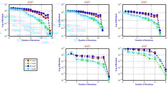
Figure 5. The residual error of the SFM${}^{\sigma }$ for approximating all polynomial equation roots used in engineering application 4 for various fractional parameter values, namely $\varsigma =0.1,0.3,0.7,0.8,1.0$.

Table 19. Local computational order of convergence using random initial approximation.

$\mathit{f}\left(\mathit{r}\right)=-0.02590111180{\mathit{r}}^4-0.1066166681{\mathit{r}}^3-0.2099871708{\mathit{r}}^2+0.7615941560\mathit{r}$
Ini-V	Local Computational Order of Convergence
$r^{\left[0\right]}$	SFM${}^{{\sigma }_1}$	SFM${}^{{\sigma }_2}$	SFM${}^{{\sigma }_3}$	SFM${}^{{\sigma }_4}$	SFM${}^{\sigma }$
$r_{1*}^{\left[0\right]}$	5.1813	5.9243	7.7124	7.0515	7.7165
$r_{2*}^{\left[0\right]}$	7.0878	6.4985	7.4236	8.1364	7.5243
$r_{3*}^{\left[0\right]}$	4.9917	6.9404	7.0148	7.3911	7.8656
$r_{4*}^{\left[0\right]}$	5.8748	5.9874	7.5154	7.6212	8.5447
$r_{5*}^{\left[0\right]}$	6.5421	6.8748	7.7177	7.0148	8.4873
Residual errors are equal to 10${}^{-30}$ using 64 D**

Table 20. CPU-Time using random initial values for finding all polynomial roots.

$\mathit{f}\left(\mathit{r}\right)=-0.02590111180{\mathit{r}}^4-0.1066166681{\mathit{r}}^3-0.2099871708{\mathit{r}}^2$
$+\mathbf{0}.\mathbf{7615941560}\mathit{r}$
Ini-V	Computational CPU-Time in Seconds
$r^{\left[0\right]}$	SFM${}^{{\sigma }_1}$	SFM${}^{{\sigma }_2}$	SFM${}^{{\sigma }_3}$	SFM${}^{{\sigma }_4}$	SFM${}^{\sigma }$
$r_{1*}^{\left[0\right]}$	3.0194	2.0514	1.0454	0.0403	0.0049
$r_{2*}^{\left[0\right]}$	2.0120	1.0314	1.0028	0.0644	0.0070
$r_{3*}^{\left[0\right]}$	2.1114	1.0141	2.0061	0.0749	0.0031
$r_{4*}^{\left[0\right]}$	1.3231	1.0804	1.0078	0.0409	0.0090
$r_{5*}^{\left[0\right]}$	1.7300	1.0761	1.0078	0.0741	0.0093
Maximum CPU-Time is equal to 2.1254 using 64 D**

The approximate local computational order of convergence is shown in Table 19. As the fractional parameter values increase from 0.1 to 1.0, the approximate local computational order of convergence increases.

Table 20 displays the computational CPU time in seconds required to approximate all roots of the polynomial equation used in application 4 using the fractional simultaneous scheme.

Convergence rates increase as the following initial estimations are sufficiently adjusted to the exact answer of engineering application 4:

$$r_1^{\left[0\right]}=0.2,r_2^{\left[0\right]}=1.4,r_3^{\left[0\right]}=-2.8+3.0i,r_4^{\left[0\right]}=-2.8-3.0i.$$

are chosen as initial guessed values.

Table 21 shows how the convergence order and accuracy of the fractional simultaneous scheme increase when we use initial guessed values close to the exact root. The residual error computed by the numerical schemes increased as we increased the fractional parameter value from 0.1 to 1.0.

Table 21. Determination of all polynomial equation roots.

Methods	SFM${}^{{\mathit{\sigma }}_1}$	SFM${}^{{\mathit{\sigma }}_2}$	SFM${}^{{\mathit{\sigma }}_3}$	SFM${}^{{\mathit{\sigma }}_4}$	SFM${}^{\mathit{\sigma }}$
Error it	$\vartheta =09$	$\vartheta =09$	$\vartheta =08$	$\vartheta =08$	$\vartheta =05$
CPU	0.0141	0.717	0.262	0.092	0.073
$e_1^{\left[\vartheta \right]}$	$9.1\times {10}^{-4}$	$0.5\times {10}^{-4}$	$0.1\times {10}^{-12}$	$5.7\times {10}^{-39}$	$9.3\times {10}^{-45}$
$e_2^{\left[\vartheta \right]}$	$1.0\times {10}^{-4}$	$2.6\times {10}^{-4}$	$9.1\times {10}^{-16}$	$5.1\times {10}^{-25}$	$0.3\times {10}^{-41}$
$e_3^{\left[\vartheta \right]}$	$6.2\times {10}^{-4}$	$2.6\times {10}^{-4}$	$9.1\times {10}^{-16}$	$4.5\times {10}^{-20}$	$8.8\times {10}^{-48}$
$e_4^{\left[\vartheta \right]}$	$2.1\times {10}^{-2}$	$0.2\times {10}^{-2}$	$9.9\times {10}^{-16}$	$7.2\times {10}^{-37}$	$0.5\times {10}^{-42}$
${\rho }_i^{[\vartheta -1]}$	2.1864	2.5002	4.0481	5.5872	7.19212

6. Conclusions

• In order to approximate all roots of nonlinear equations, a new fractional parallel approach with convergence orders of $3\varsigma +5$ is presented. The global convergence behavior of the fractional parallel schemes is demonstrated using a variety of random starting estimates of SFM${}^{{\sigma }_1}-$SFM${}^{{\sigma }_4},$ SFM${}^{\sigma }$.
• The numerical results of the engineering applications from Table 1, Table 2, Table 3, Table 4, Table 5, Table 6, Table 7, Table 8, Table 9, Table 10, Table 11, Table 12, Table 13, Table 14, Table 15, Table 16, Table 17, Table 18, Table 19, Table 20 and Table 21 and Figure 1, Figure 2, Figure 3, Figure 4 and Figure 5 clearly show the efficiency of the newly developed methods in terms of CPU-time, computational error, maximum residual error, and local computational order of convergence (LCOC). The acceleration of the convergence rate is observed when the initial approximations close to the exact roots are selected as shown in Table 6, Table 11, Table 16 and Table 21.
• In the future, higher-order parallel iterative approaches for solving (1) will be developed to handle more difficult engineering problems using fractional derivatives of Riemann–Liouville and Grunwald–Letnikov types.

References

- Traub, J.F. Iterative Methods for the Solution of Equations; Prentice-Hall: Englewood Cliffs, NJ, USA, 1964. [Google Scholar]
- Jarratt, P. Some efficient fourth order multiple methods for solving equations. BIT 1969, 9, 119–124. [Google Scholar] [CrossRef]
- King, R. A family of fourth order methods for nonlinear equations. SIAM J. Numer. Anal. 1973, 10, 876–879. [Google Scholar] [CrossRef]
- Ostrowski, A.M. Solution of Equation in Euclidean and Banach Space, 3rd ed.; Academic Press: New York, NY, USA, 1973. [Google Scholar]
- Chun, C. Some fourth-order iterative methods for solving nonlinear equations. Appl. Math. Lett. 2008, 195, 454–456. [Google Scholar] [CrossRef]
- Weierstrass, K. Neuer Beweis des Satzes, dass jede ganze rationale Function einer Verän derlichen dargestellt werden kann als ein Product aus linearen Functionen derselben Verän derlichen. Sitzungsberichte KöNiglich Preuss. Akad. Der Wiss. Berl. 1981, 2, 1085–1101. [Google Scholar]
- Kanno, S.; Kjurkchiev, N.V.; Yamamoto, T. On some methods for the simultaneous determination of polynomial zeros. Japan J. Appl. Math. 1995, 13, 267–288. [Google Scholar] [CrossRef]
- Proinov, P.D.; Cholakov, S.I. Semilocal convergence of Chebyshev-like root-finding method for simultaneous approximation of polynomial zeros. Appl. Math. Comput. 2014, 236, 669–682. [Google Scholar] [CrossRef]
- Mir, N.A.; Muneer, R.; Jabeen, I. Some families of two-step simultaneous methods for determining zeros of nonlinear equations. ISRN Appl. Math. 2011, 2011, 817174. [Google Scholar] [CrossRef]
- Farmer, M.R. Computing the Zeros of Polynomials Using the Divide and Conquer Approach; Department of Computer Science and Information Systems; Birkbeck: London, UK, 2014. [Google Scholar]
- Nourein, A.W. An improvement on Nourein’s method for the simultaneous determination of the zeroes of a polynomial (an algorithm). J. Comput. Appl. Math. 1977, 3, 109–112. [Google Scholar] [CrossRef]
- Aberth, O. Iteration methods for finding all zeros of a polynomial simultaneously. Math. Comput. 1973, 27, 339–344. [Google Scholar] [CrossRef]
- Cholakov, S.I.; Vasileva, M.T. A convergence analysis of a fourth-order method for computing all zeros of a polynomial simultaneously. J. Comput. Appl. Math. 2017, 321, 270–283. [Google Scholar] [CrossRef]
- Consnard, M.; Fraigniaud, P. Finding the roots of a polynomial on an MIMD multicomputer. Parall. Comput. 1990, 15, 75–85. [Google Scholar] [CrossRef]
- Petković, M.S.; Petković, L.D.; Džunić, J. On an efficient method for the simultaneous approximation of polynomial multiple roots. Appl. Anal. Disc. Math. 2014, 8, 73–94. [Google Scholar] [CrossRef]
- Rafiq, N.; Shams, M.; Mir, N.A.; Gaba, Y.U. A highly efficient computer method for solving polynomial equations appearing in Engineering Problems. Math. Probl. Eng. 2023, 2021, 9826693. [Google Scholar] [CrossRef]
- Shams, M.; Rafiq, N.; Kausar, N.; Agarwal, P.; Park, C.; Mir, N.A. On iterative techniques for estimating all roots of nonlinear equation and its system with application in differential equation. Adv. Differ. Equ. 2021, 2021, 480. [Google Scholar] [CrossRef]
- Kyncheva, V.K.; Yotov, V.V.; Ivanov, S.I. Convergence of Newton, Halley and Chebyshev iterative methods as methods for simultaneous determination of multiple polynomial zeros. Appl. Numer. Math. 2017, 112, 146–154. [Google Scholar] [CrossRef]
- Nedzhibov, H. Iterative methods for simultaneous computing arbitrary number of multiple zeros of nonlinear equations. Int. J. Comp. Math. 2013, 90, 994–1007. [Google Scholar] [CrossRef]
- Sendov, B.L.; Andreev, A.; Kjurkchiev, N. Numerical solution of polynomial equations. Handb. Numer. Anal. 1994, 3, 625–778. [Google Scholar]
- Kyurkchiev, N.; Iliev, A. A general approach to methods with a sparse Jacobian for solving nonlinear systems of equations. Serdica Math. J. 2007, 33, 433–448. [Google Scholar]
- Shams, M.; Kausar, N.; Agarwal, P.; Oros, G.I. On Efficient Fractional Caputo-type Simultaneous Scheme for Finding all Roots of polynomial equations. Fractals 2023, 6, 2340075. [Google Scholar] [CrossRef]
- Dimitrov, Y.; Georgiev, S.; Todorov, V. Approximation of Caputo Fractional Derivative and Numerical Solutions of Fractional Differential Equations. Fractal Fract. 2023, 7, 750. [Google Scholar] [CrossRef]
- Shams, M.; Kausar, N.; Agarwal, P.; Shah, M.A. On family of Caputo-Type fractional numerical scheme for solving polynomial. Appl. Math. Sci. Eng. 2023, 31, 2181959. [Google Scholar] [CrossRef]
- Oliveira, D.E.C.; Tenreiro Machado, J.A. A review of definitions for fractional derivatives and integral. Math. Probl. Eng. 2014, 2014, 238459. [Google Scholar] [CrossRef]
- Oldham, K.; Spanier, J. The Fractional Calculus Theory and Applications of Differentiation and Integration to Arbitrary Order; Elsevier: Amsterdam, The Netherlands, 1974. [Google Scholar]
- Kukushkin, M.V. Abstract fractional calculus for m-accretive operators. arXiv 2019, arXiv:1901.06118. [Google Scholar] [CrossRef]
- Samko, S.G.; Kilbas, A.A.; Marichev, O.I. Fractional Ntegrals and Derivatives: Theory and Applications; Gordon and Breach Science Publishers: Philadelphia, PA, USA, 1993. [Google Scholar]
- Shams, M.; Carpentieri, B. Efficient Inverse Fractional Neural Network-Based Simultaneous Schemes for Nonlinear Engineering Applications. Fractal. Fract. 2023, 7, 849. [Google Scholar] [CrossRef]
- Odibat, Z.M.; Shawagfeh, N.T. Generalized Taylor’s formula. Appl. Math. Comput. 2007, 186, 286–293. [Google Scholar] [CrossRef]
- Akgül, A.; Cordero, A.; Torregrosa, J.R. A fractional Newton method with 2th-order of convergence and its stability. Appl. Math. Lett. 2019, 98, 344–351. [Google Scholar] [CrossRef]
- Torres-Hernandez, A.; Brambila-Paz, F. Sets of fractional operators and numerical estimation of the order of convergence of a family of fractional fixed-point methods. Fractal Fract. 2021, 4, 240. [Google Scholar] [CrossRef]
- Cajori, F. Historical note on the Newton-Raphson method of approximation. Am. Math. Mon. 1911, 18, 29–32. [Google Scholar] [CrossRef]
- Kumar, P.; Agrawal, O.P. An approximate method for numerical solution of fractional differential equations. Signal Process. 2006, 86, 2602–2610. [Google Scholar] [CrossRef]
- Candelario, G.; Cordero, A.; Torregrosa, J.R. Multipoint fractional iterative methods with (2 + 1) th-order of convergence for solving nonlinear problems. Mathematics 2020, 8, 452. [Google Scholar] [CrossRef]
- Proinov, P.D.; Vasileva, M.T. On the convergence of high-order Ehrlich-type iterative methods for approximating all zeros of a polynomial simultaneously. J. Ineq. Appl. 2015, 2015, 336. [Google Scholar] [CrossRef]
- Chu, Y.; Rafiq, N.; Shams, M.; Akram, S.; Mir, N.A.; Kalsoom, H. Computer methodologies for the comparison of some efficient derivative free simultaneous iterative methods for finding roots of non-linear equations. Comput. Mater. Cont. 2020, 66, 275–290. [Google Scholar] [CrossRef]
- Naseem, A.; Rehman, M.A.; Abdeljawad, T. Computational methods for non-linear equations with some real-world applications and their graphical analysis. Intell. Autom. Soft Comput. 2021, 30, 1–14. [Google Scholar] [CrossRef]
- Akin-Bohnera, E.; Hoackerb, J. Oscillation properties of an Emden-Fowler type equation on discrete time scales. J. Diff. Equ. Appl. 2003, 9, 603612. [Google Scholar] [CrossRef]
- Shams, M.; Kausar, N.; Yaqoob, N.; Arif, N.; Addis, G.M. Techniques for finding analytical solution of generalized fuzzy differential equations with applications. Complexity 2023, 2023, 3000653. [Google Scholar] [CrossRef]
- Zill, D.G. Differential Equations with Boundary-Value Problems; Cengage Learning: Boston, MA, USA, 2016. [Google Scholar]
- Chapra, S. EBOOK: Applied Numerical Methods with MATLAB for Engineers and Scientists; McGraw Hill: New York, NY, USA, 2011. [Google Scholar]
Disclaimer/Publisher’s Note: The statements, opinions and data contained in all publications are solely those of the individual author(s) and contributor(s) and not of MDPI and/or the editor(s). MDPI and/or the editor(s) disclaim responsibility for any injury to people or property resulting from any ideas, methods, instructions or products referred to in the content. |
© 2023 by the authors. Licensee MDPI, Basel, Switzerland. This article is an open access article distributed under the terms and conditions of the Creative Commons Attribution (CC BY) license (https://creativecommons.org/licenses/by/4.0/).