Article

Mathematical Modeling of Periodic Outbreaks with Waning Immunity: A Possible Long-Term Description of COVID-19

by
Alex Viguerie
1,
Margherita Carletti
2,*,
Guido Silvestri
3 and
Alessandro Veneziani
4,5
1
Division of Mathematics, Gran Sasso Science Institute, Viale Francesco Crispi 7, 67100 L’Aquila, AQ, Italy
2
Department of Pure and Applied Sciences, University of Urbino C. Bo, Piazza della Repubblica 13, 61029 Urbino, PU, Italy
3
Department of Pathology and Laboratory Medicine, Emory University School of Medicine, Atlanta, GA 30322, USA
4
Department of Mathematics, Emory University, 400 Dowman Drive NE, Atlanta, GA 30322, USA
5
Department of Computer Science, Emory University, 400 Dowman Drive NE, Atlanta, GA 30322, USA
*
Author to whom correspondence should be addressed.
Mathematics 2023, 11(24), 4918; https://doi.org/10.3390/math11244918
Submission received: 31 August 2023 / Revised: 7 November 2023 / Accepted: 5 December 2023 / Published: 11 December 2023
(This article belongs to the Section Mathematical Biology)

Abstract

:
The COVID-19 pandemic is still ongoing, even if the emergency is over, and we now have enough data to analyze the outbreak over a long timeline. There is evidence that the outbreak alternates periods of high and low infections. Retrospectively, this can help in understanding the nature of an appropriate mathematical model for this dramatic infection. The periodic behavior may be the consequence of time-dependent coefficients related to seasonal effects and specific political actions, or an intrinsic feature of the model. The present paper relies on the assumption that the periodic spikes are an intrinsic feature of the disease, and, as such, it should be properly reflected in the mathematical model. Based on the concept of waning immunity proposed for other pathologies, we introduce a new model with (i) a compartment for weakly immune people subject to immunity booster, represented by a non-linear term; (ii) discrimination between individuals infected/vaccinated for the first time, and individuals already infected/vaccinated, undergoing to new infections/doses. We analyze some preliminary properties of our model, called SIRW2, and provide a proof-of-concept that it is capable of reproducing qualitatively the long-term oscillatory behavior of COVID-19 infection.
MSC:
92-10; 37M05; 92D30

1. Introduction

It has been years now since the world experienced the COVID-19 pandemic. We have enough data to identify some patterns in the evolution of the outbreak over time. In particular, in many situations it is evident that the outbreak features oscillations, showing an alternating behavior of high and low infection. For example, in Figure 1, we plot the infected curve in Italy, Georgia (U.S. State), Brazil, and Japan over the entire time span of the pandemic (February 2020–October 2023) at the time of writing. These countries/states are distinct culturally, geographically, and demographically [1,2]. Despite these differences and the different policies enforced to face the pandemic, the patterns are very similar, and a Fourier spectral analysis of the data shows that the dominant frequencies in each case are between 8 months 1 and 6 months 1 —see Figure 1. Whether this is the effect of a seasonal infection rate, government measures, or a structural nature of the pandemic is currently an open question.
The calibration of mathematical models with a predictive purpose can be widely educated by the answer to this question. In particular, if we assume that the periodic behavior is a structural feature of the pandemic, a mathematical model should reflect this in the nature of its asymptotic solutions. On the contrary, if the periodicity is the result of seasonality or government responses to the pandemic only (such as lockdowns and masking mandates), the model should incorporate this effect in its parameter calibration.
In the majority of work modeling COVID-19, this latter assumption is employed. Such works typically adopt classical compartmental models, sophisticated variants of SIR (Susceptible-Infected-Recovered, see [3,4] for detailed discussion), and its derivations. These models may lead to excellent short-term quantitative predictions; however, they generally do not yield periodic behaviors when using time-independent parameters [5] over longer time scales. In order to recover the observed behavior, these models must employ time-dependent parameter fitting (see, among the others, [6,7,8,9,10]).
This paper follows a different direction, being more concerned with the qualitative agreement between the data and the asymptotic behavior of a mathematical model. The strong similarity among the data from different Countries suggests that the behavior of the solution is the consequence of the intrinsic dynamics of the disease more than of seasonal or policy time-dependent effects. The wavy pattern displayed by the data informs the modeler about critical aspects that should be included in a mathematical description, before the tuning of parameter values. We aim to provide a mathematical description that elucidates basic qualitative mechanisms of the outbreak, acknowledging that behavioral, seasonal, and other external aspects (e.g., higher infectivity in winter, lower in summer, different infectivity of different variants, lockdowns) impact the pattern quantitatively. As a matter of fact, intrinsic asymptotic dynamics and time-dependent parameterizations are not mutually exclusive and the data we observe are most likely a combination of different effects on long and short time scales.
Our starting point here is the concept of waning immunity advocated for other pathologies [11], and considered for COVID-19 with different mathematical descriptions [12,13,14,15]. The basic idea is that the immunity induced by recovery or vaccination declines over time. This was largely demonstrated by the cases of reinfection/infection-after-vaccination documented for the COVID-19 outbreak. However, we make here the point that the reduction in the immunity does not follow a simple pattern because there is an immunity booster effect: an individual with a declining immunity exposed to an infected person may obtain a beneficial effect, reinforcing (or boosting) the immune system. This leads to a model called SIRW, where the compartment W (Waning) added to the classical SIR denotes the “weakly immune” individuals that may go back to the Susceptible compartment or obtain an immunity booster by contact with infected or vaccination [16,17]. The mathematical description of this phenomenon leads to a new non-linear term in the equations, still based on a kinetic argument similar to the one in predator-prey and basic SIR models [5]. To the authors’ best knowledge, this specific aspect was never considered for COVID-19. It has been demonstrated [11] that this new nonlinear term leads the system to have limit cycles (i.e., asymptotic periodic solutions) for particular combinations of the parameters. One of the important aspects of the model is its “multiscale-in-time” nature, where the natural growth of the population (according to a Malthusian model) is, in fact, a slower process compared to the infection/vaccination rate.
We propose here an extension of this model specifically designed for the COVID-19 pandemic. We further stratify all four SIRW compartments into “never previously exposed” and “previously exposed” subpopulations. The rationale is that, while a vaccinated or previously infected individual may lose their immunity from infection over time, some baseline protection is nonetheless maintained; the illness is less likely to be severe and is more likely to pass quickly. For COVID-19, this is supported by different lines of evidence, including evidence that persons recently infected with the human coronaviruses HKU1, OC43, NL63, and 229E had significant partial immunity to COVID-19 infection [18,19,20,21]. This motivates the use of different parameters for the dynamics of “previously unexposed” vs. “previously exposed” populations. A similar concept in the case of pertussis (with no immunity booster) was advocated in [22]. As the model is formally a duplication of the four SIRW compartments (plus the Deceased), we call it SIRW2 (SIRWsquare).
We provide a preliminary proof-of-concept that the SIRW2 model can actually describe the wavy behavior even in the absence of a time-dependent calibration of the parameters, and to provide some qualitative properties of the solution of the differential system. Our results suggest that this model can potentially provide a reliable long-term description of the COVID-19 outbreak.
The document is organized as follows. We first introduce the waning immunity and explain the SIRW model (introduced in [17] and further studied in [11,16]) in order to describe the immune-boosting process and provide the motivation behind the SIRW2 model. We then introduce the full SIRW2 model, providing the model equations, a description of the dynamics they are intended to model, and a complete list of the relevant parameters and their purpose. We prove the positivity and the boundedness of the solution. We then numerically demonstrate that this model may, in principle, reproduce wave-like dynamics even with time-constant parameters.
We conclude with a series of perspectives on future steps in terms of both theoretical analysis and validation. We argue that the periodic dynamics of COVID-19 pandemic, being intrinsic to the nature of the infection, provide the opportunity to gain critical insights into the modeling aspects required by a reliable mathematical description and ultimately, a deep understanding of this infection.

2. The Mathematical Model
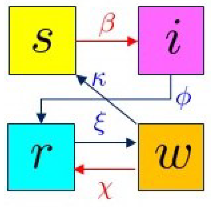
2.1. The SIRW Model

The SIRW model introduced in [17] and studied in [11,16] considers the susceptible s, infected i, recovered r, and waning w compartments and reads as follows (the dot here denotes differentiation in time):
s ˙ = β s i + κ w , i ˙ = β s i ϕ i , r ˙ = ϕ i ξ r + χ i w , w ˙ = ξ r χ i w κ w ,
together with the initial conditions s ( 0 ) = s 0 , i ( 0 ) = i 0 , r ( 0 ) = r 0 , w ( 0 ) = w 0 (see Figure 2). A full list of the variables and parameters in (1) is provided in Table 1. The block diagram in Figure 2 describes the passage of individuals throughout the four compartments. A susceptible individual (s), upon contact with an infected individual i, may become infected. The dynamics are mathematically similar to the classical predator–prey system, resulting in a term proportional to s i . Infected individuals recover with a rate ϕ , moving into the r compartment, where they acquire immunity from infection. At a rate of ξ , recovered individuals begin to lose their immunity, entering the waning compartment w.
While the immunity is waning, two things can happen.
(i)
The waning individual can come into contact with an infected individual again, with contact rate χ , boosting their immunity, returning them to the r compartment; this is again described by a predator-prey term, proportional to w i .
(ii)
The waning individual loses their immunity with no additional contact with the virus and returns to the s compartment at rate κ .
In [11,17], the model (1) was shown to admit periodic-orbit solutions in time using the Geometric Singular Perturbation Theory. Even if no constructive arguments were provided to identify the values of the parameters that give periodicity, this result is critical as it suggests a correspondence between the modeled immune-boosting process and the possible oscillatory dynamics of COVID-19 data.
In Figure 3, we demonstrate the occurrence of a limit cycle for the values of the parameters reported in Table 1 (Periodic). An empirical trial-and-error approach identified these values, yet they corroborate the theoretical results of [11].
By changing the parameter ξ , it is also possible to obtain an asymptotic equilibrium solution associated with damped oscillations (Table 1, Steady equilibrium), shown on the bottom row of Figure 3.
What we were unable to reproduce in this model is the occurrence of spikes with a non-monotone behavior in time, i.e., spikes with larger top values than the previous ones, as we found, in fact, in the available data, see Figure 1. Additionally, the SIRW model shown does not account for any durable immune processes; with the loss of immunity, an individual is returned to the susceptible compartment as if the initial infection never occurred. For this reason, we elaborated a more accurate mathematical description.

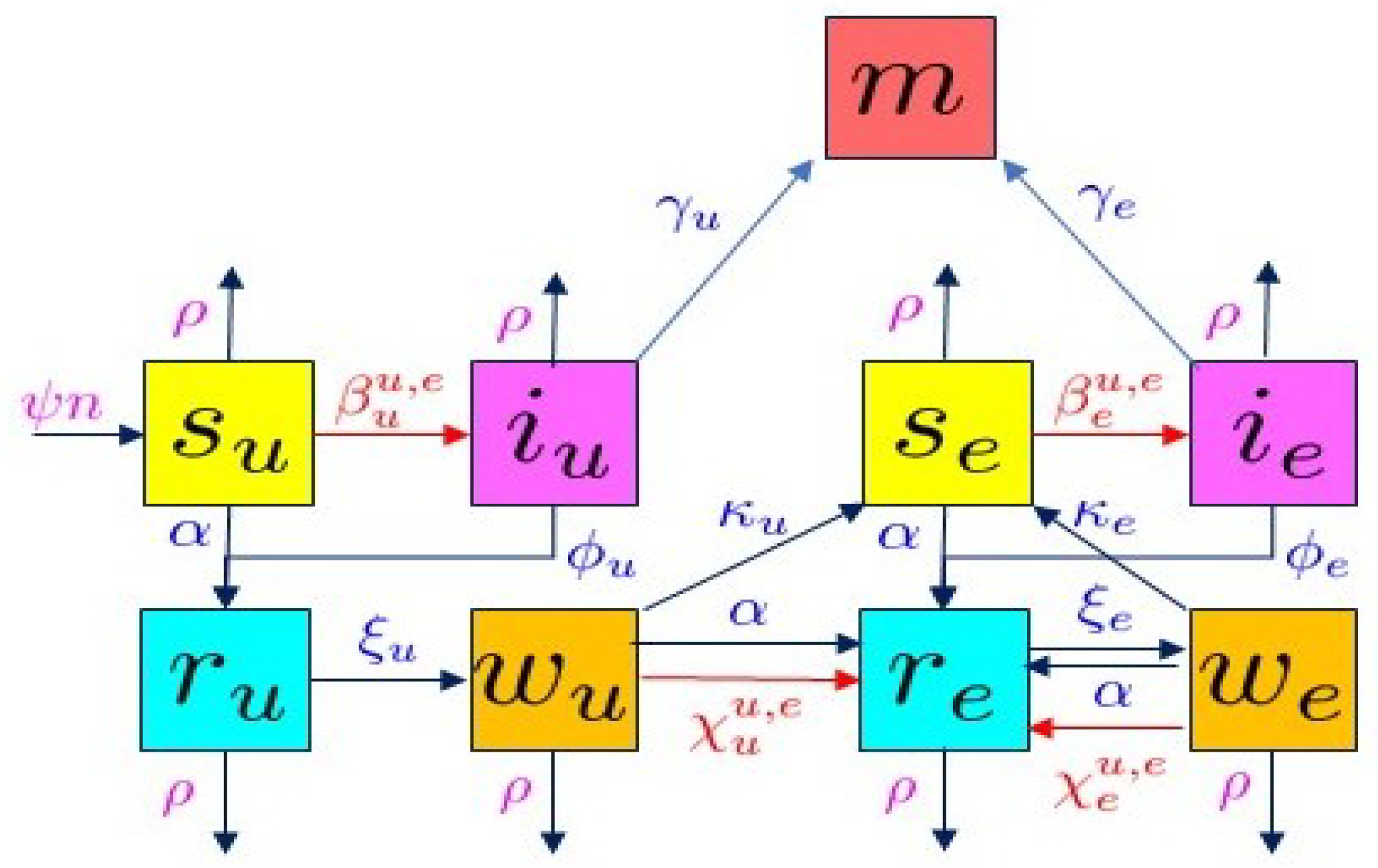
2.2. The SIRW2 Model

The model (1) does not consider vaccinations and does not consider mortality from the disease. The addition of several new terms for vaccination and mortality, as well as an additional compartment for the deceased, is sufficient for their inclusion.
The more important modification necessary, however, is that the loss of immunity is not a complete and total elimination of all immunity. For instance, in reality, individuals maintain some baseline of immunological protection in the form of Memory B- cells [23,24]. These protections both protect against severe disease and lead to a faster recovery process upon reinfection when compared to infection in an individual with no prior immunological protection. To this end, we introduce an extension of (1) incorporating these crucial effects: vaccination, disease mortality, and the distinction between populations with and without prior immunological exposure (a version of (1) incorporating vaccination was studied in [11,17]). To model vaccination, we add a vaccination term, which can both grant and boost immunity (i.e., enable the movement s r and w r ). For the addition of mortality, we add another compartment, denoted m (for ‘mortality’), to track deceased individuals. Finally, we stratify the populations based on whether or not they have prior immunological protection, either from vaccination or prior infection. We also incorporate a Malthus demographic independent of the disease into the model. The extended model, which we denote by SIRW2 (SIRW-square), reads:
s ˙ u = β u u s u i u β u e s u i e ( α + ρ ) s u + ψ n i ˙ u = β u u s u i u + β u e s u i e ( ϕ u + γ u + ρ ) i u r ˙ u = ϕ u i u + α s u ( ξ u + ρ ) r u w ˙ u = ξ u r u χ u e w u i e χ u u w u i u ( κ u + α + ρ ) w u s ˙ e = β e u s e i u β e e s e i e + κ u w u + κ e w e ( α + ρ ) s e i ˙ e = β e u s e i u + β e e s e i e ( ϕ e + γ e + ρ ) i e r ˙ e = ϕ e i e + χ e e w e i e + χ e u w e i u + χ u e w u i e + χ u u w u i u + α w u + α w e + α s e ( ξ e + ρ ) r e , w ˙ e = ξ e r e χ e e w e i e χ e u w e i u ( κ e + α + ρ ) w e , m ˙ = γ u i u + γ e i e ,
together with the initial conditions s u ( 0 ) = s u , 0 , i u ( 0 ) = i u , 0 , r u ( 0 ) = r u , 0 , w u ( 0 ) = w u , 0 , s e ( 0 ) = s e , 0 , i e ( 0 ) = i e , 0 , r e ( 0 ) = r e , 0 , w e ( 0 ) = w e , 0 , m ( 0 ) = m 0 (see Figure 4). Here, n = s u + i u + r u + w u + s e + i e + r e + w e is the size of the living population. The subscript u indicates ‘unexposed’, meaning this class of individuals has not been previously infected with, or vaccinated against, the disease. The subscript e indicates ‘previously exposed’, meaning that this class of individuals has been infected previously, or vaccinated against, the disease. Verbally, the model (2) describes the population of persons who have never been infected with the disease s u , who may become infected via contact with either a first-time infected ( i u ) or reinfected ( i e ) person. After moving to the first-infection compartment i u , a person may recover (with rate ϕ u ) or die (rate γ u ). Assuming recovery, the movement is into the compartment r u , indicating recovery with immunity. Alternatively, an individual may be vaccinated (with rate α ) and move directly from s u to r u without any previous infection.
Once in the recovered state r u , an individual begins to lose immunity, and, at a rate of ξ u , the individual moves to the waning state w u . In the waning state, a few things can happen:
(i)
An individual can come into contact with an infected individual (either i u or i e ), with contact rate χ u , χ e , respectively, boosting the immunity and moving directly to the compartment r e ;
(ii)
An individual can receive a vaccine booster (rate α ), also boosting their immunity and moving to r e ;
(iii)
In the absence of additional contact with the virus, in the form of exposure to an infected individual or a vaccine booster, the immunity can be lost with a rate κ u . In this case, the switch is to the compartment s e .
From there, the model progression works similarly to in the first-infection (sub-scripted with u) case, in the movement between the i e , r e , and w e states. However, the previously-exposed infection progression differs from the first-time infection progression in that the relevant parameters are different. For most diseases, we postulate that:
(iv)
The mortality rate is substantially lower: γ e << γ u ;
(v)
The recovery rate is substantially higher: ϕ e >> ϕ u .
This is in line with observation and general consensus. Our model evidence also suggests that
(a)
immunity is lost more quickly after reinfection: ξ e > ξ u ;
(b)
however, it is also boosted more easily among those with prior immunity: χ e e > χ u e , χ e u > χ u u .
The compartment m depends on the other populations, yet it has no effect on their dynamics. However, we want to include it in the system, as in reality the number of deceased for the pandemic is a pretty accurate measure and we will compare our results with available data. Notice that, under the standard assumption ψ = ρ , summing up all the equations we have (thanks to Proposition 1 below)
n ˙ = γ u i u γ e i e ( γ u + γ e ) n
so we can conclude that
n ( 0 ) e ( γ u + γ e ) t n ( t ) n ( 0 )
and m ( t ) = n ( 0 ) n ( t ) .
A full list and short description of the different variables, parameters, and their units are given in Table 2.

2.3. Basic Properties of the SIRW2 Model

A deep mathematical analysis of the differential system (2) is out of the scope of the present paper. We present here some preliminary results.
We recall first the following result [25,26]. The original result refers to a case with delay, we particularize it to the case with no delay.
Lemma 1. 
Given a system for i = 1 , 2 , , N , with non-negative initial conditions
X ˙ i = f i ( t , X 1 , X 2 , , X N ) ,
with f i ( t , X 1 , X 2 , , X N ) C ( R , C N ) . If f i ( t , X 1 , X 2 , , X i 1 , 0 , X i + 1 , , X N ) 0   X j 0 , then [ X 1 , X 2 , , X N ] are continuous and non-negative t > 0 .
Proposition 1 
(Positiveness and boundedness of the solution). If the initial conditions of system (2) are non-negative, the entire solution is non-negative and bounded in the region [ 0 , n ] 9 .
Proof. 
Non-negativity of the solution can be approached in different ways (see, e.g., [27,28,29,30,31]).
Here, we follow an approach based on the Lemma. It is enough to verify that each right-hand-side of (2) is non-negative when the relative function is 0, and the other compartments are non-negative. In our case:
s ˙ u , s u = 0 = ψ n > 0 i ˙ u , i u = 0 = β u e s u i e 0 r ˙ u , r u = 0 = ϕ u i u + α s u 0 w ˙ u , w u = 0 = ξ u r u 0 s ˙ e , s e = 0 = κ u w u + κ e w e 0 i ˙ e , i e = 0 = β e u s e i u 0 r ˙ e , r e = 0 = ϕ e i e + χ e e w e i e + χ e u w e i u + χ u e w u i e + χ u u w u i u + α w u + α w e 0 w ˙ e , w e = 0 = ξ e r e 0 m ˙ = 0 = γ u i u + γ e i e 0
At this point, being n = s u + i u + r u + w u + s e + i e + r e + w e , each term on the right is bounded. Consequently, m n ( 0 ) . In conclusion, all the populations belong to the set [ 0 , n ( t ) ] 9 [ 0 , n ( 0 ) ] 9 . □
In the case of n constant, i.e., γ u = γ e = 0 (so for m ( 0 ) = 0 , m 0 ), we can also identify a possible disease-free equilibrium, i.e., an equilibrium s.t. i u = i e = 0 . By direct inspection, the disease-free equilibrium solves
0 = α s u + ψ n ρ s u , 0 = ϕ u i u γ u i u ρ i u , 0 = α s u ξ u r u ρ r u , 0 = ξ u r u κ u w u α w u ρ w u , 0 = κ u w u + κ e w e α s e ρ s e , 0 = ϕ e i e γ e i e ρ i e , 0 = ξ e r e + α w u + α w e + α s e ρ r e , 0 = ξ e r e κ e w e α w e ρ w e .
so that the second and sixth equations are trivially true. Then, we find the equilibrium
s u = ψ n α + ρ , r u = α s u ξ u + ρ , w u = ξ u r u κ u + α + ρ , w e = ρ ξ e ( κ e + α + ρ ) + ρ 1 + κ e α + ρ 1 α 1 + κ u α + ρ w u , r e = κ e + α + ρ ξ e w e , s e = κ u ρ + α w u + κ e ρ + α w e .
The investigation of the stability of this point will be the subject of a forthcoming work. Here, we are more interested in the transient as well as in the existence of limit cycles. We will investigate these aspects in the numerical section.

2.4. Local Sensitivity Equations

We write the equations for the sensitivity on the booster rate χ u u , i.e., on the efficiency of the immunization when an individual with waning immunity meets an infected in the first-infection group. The sensitivities are defined as the first derivatives of the population with respect to the corresponding parameter ( χ u u in this case) and are denoted by σ where ∗ is the compartment we are considering. By direct differentiation, we obtain:
σ ˙ s u = β u u σ s u i u β u u s u σ i u β u e σ s u i e β u e s u σ i e ( α + ρ ) σ s u , σ ˙ i u = β u u σ s u i u + β u u s u σ i u + β u e σ s u i e + β u e s u σ i e ( ϕ u + γ u + ρ i u ) σ i u , σ ˙ r u = ϕ u σ i u + α σ s u ξ u σ r u + α σ w u ρ σ r u , σ ˙ w u = ξ u σ r u χ u e σ w u i e χ u e w u σ i e χ u u σ w u i u χ u u w u σ i u w u i u ( κ u + α w u + ρ ) σ w u , σ ˙ s e = β e u σ s e i u β e e σ s e i e β e u s e σ i u β e e s e σ i e + κ u σ w u + κ e σ w e α σ s e ρ σ s e , σ ˙ i e = β e u σ s e i u + β e e σ s e i e + β e u s e σ i u + β e e s e σ i e ϕ e σ i e γ e σ i e ρ σ i e , σ ˙ r e = ϕ e σ i e ξ e σ r e + χ u e σ w u i e + χ u e w u σ i e + χ u u σ w u i u + χ u u w u σ i u + w u i u + χ e e σ w e i e + χ e u σ w e i u + χ e e w e σ i e + χ e u w e σ i u + α σ w e ρ σ r e , σ ˙ w e = ξ e σ r e χ e u σ w e i u χ e e w e σ i e χ e u w e σ i u χ e u w e σ i u κ e σ w e α σ w e ρ σ w e , σ ˙ m = γ u σ i u + γ e σ i e .
Similar equations can be obtained for the sensitivities to the other parameters. We will solve these equations contextually with the system (2) to estimate the local dependence of the solution on the value of a specific parameter.

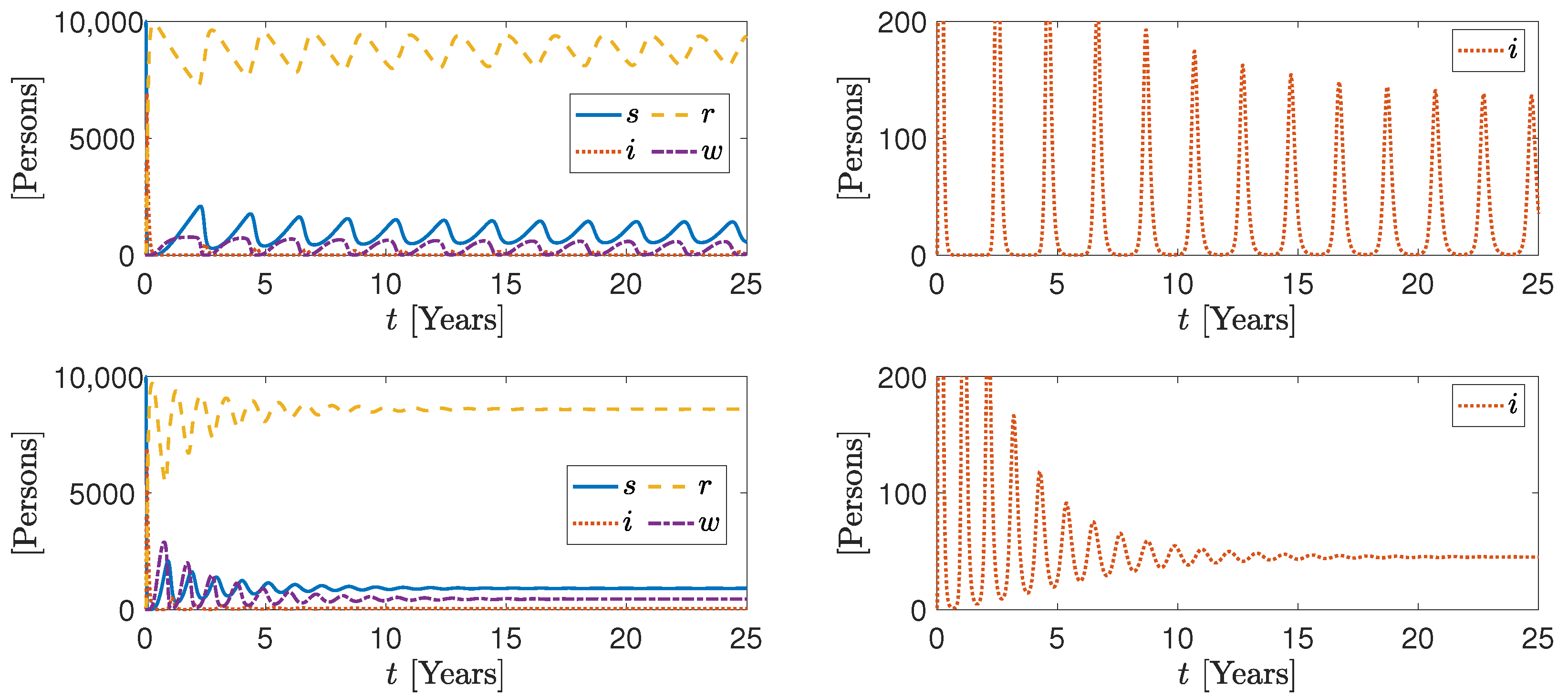
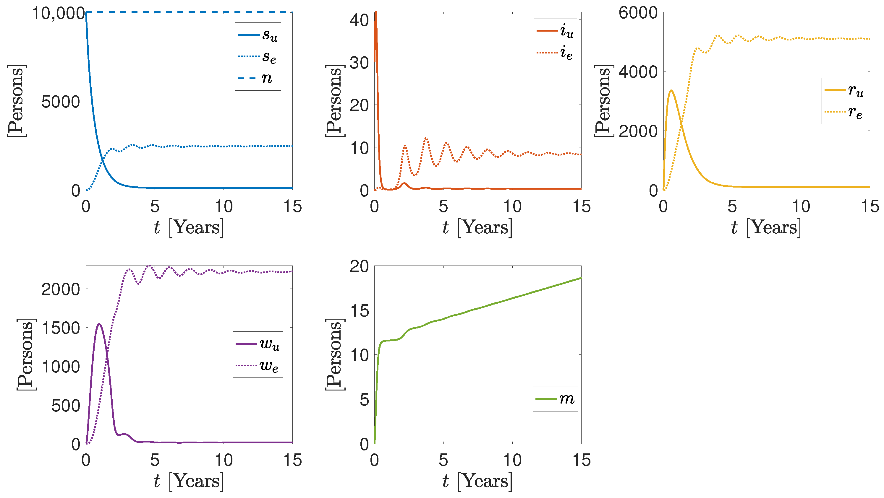
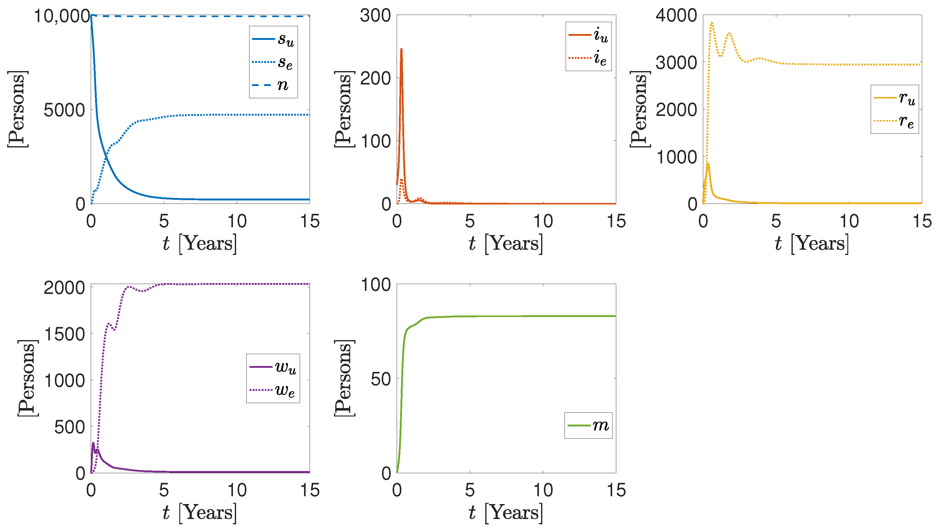
3. Numerical Results

We briefly demonstrate the model’s capability by running it for a hypothetical scenario. We take parameter values as shown in Table 3. Again, these parameters were selected with a trial and error approach to probe different possible asymptotic behaviors of our model. Therefore, these values do not necessarily correspond to any particular outbreak values, they showcase the type of solutions that (2) can admit, in particular, in the long term. The model is implemented in MATLAB R2019b [32], utilizing the ode23s solver.
We consider, in particular, three cases. In the first one, the model converges to a limit cycle. In the second one, the model converges to a constant solution with a transient featuring damped oscillations. The equilibrium is not disease-free. In the third case, the solution converges to a disease-free equilibrium.
The results in Figure 5, Figure 6 and Figure 7 pinpoint the variety of possible scenarios SIRW2 may generate depending on the different parameters. In Figure 5, we observe a limit cycle after a transient where the second spike is higher than the first one (top right and bottom left panels). The sensitivity of the infected on the parameter χ u oscillates in time (bottom right panel). This stresses the importance of an accurate parameter estimation for a reliable quantitative analysis.
In the second case, Figure 6, the oscillations are damped to an equilibrium that implies a constant number of infected in the long term. Correspondingly, we will have a relatively high number of individuals in the w e compartment (bottom-right panel).
In the third case, Figure 7, the infected compartments converge to the null solution after an initial transient.
These results confirm the versatility of SIRW2 for the possible asymptotic evolution of the outbreak. An accurate and, possibly time-dependent calibration of the parameters based on the available data will help clarify what we may expect from the evolution of COVID-19 in the coming years. However, we note from the second simulation that periodic-like behavior can continue for several years before converging to a steady-state equilibrium. It is, therefore, too early to determine whether COVID-19 will demonstrate a fully periodic behavior over the long term (as in Example 1), or will instead converge to a steady state (as in Example 2). However, the SIRW2 is capable of producing either possible outcome.

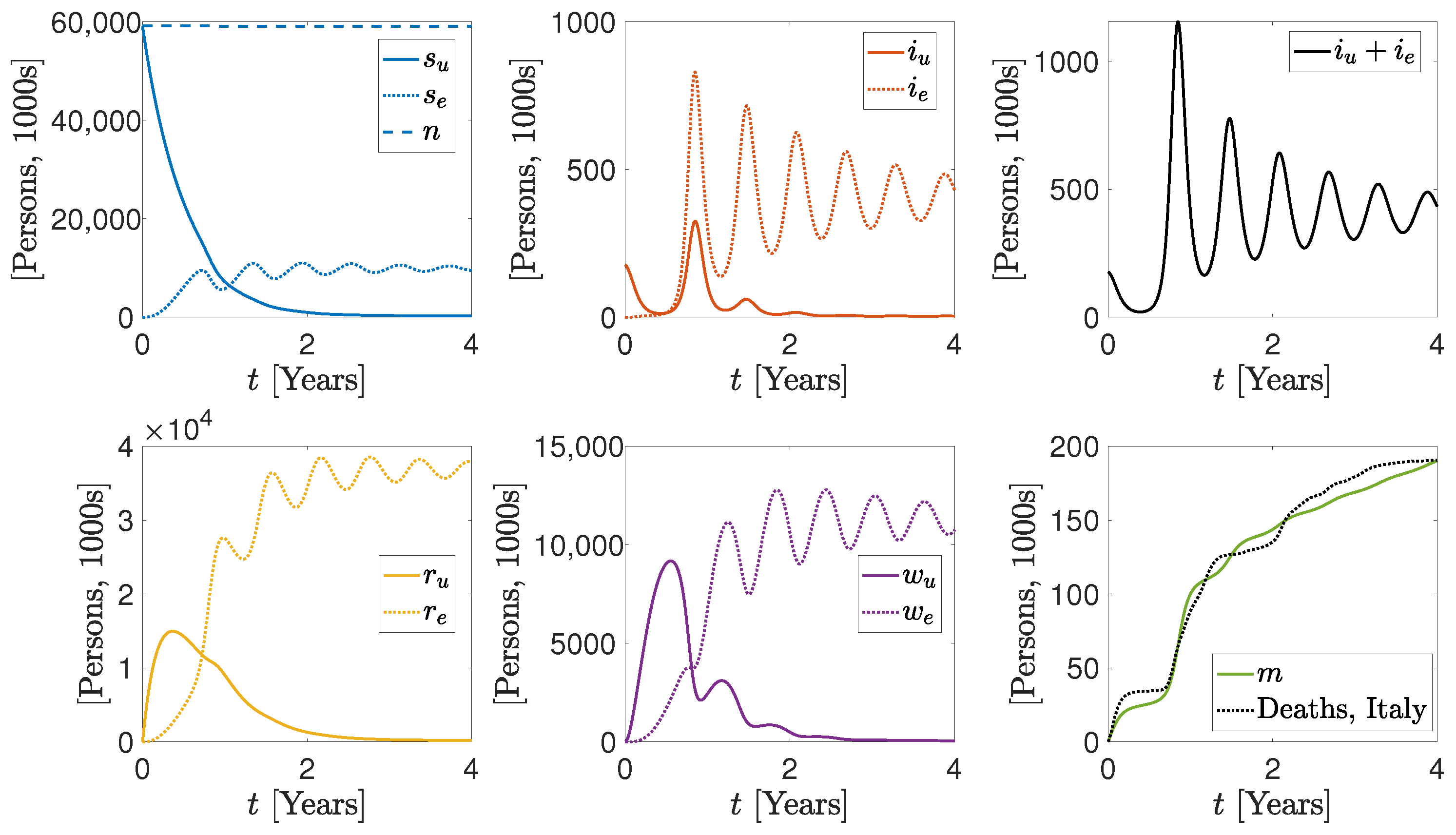
More Realistic Cases

We conclude our numerical demonstrations by showing that the SIRW2 model can, with fixed-time parameters, recreate dynamics that align well with surveillance data. Using the parameter values in Table 4 the SIRW2 model produces the results shown in Figure 8 and Figure 9. The last panel of these figures displays the deceased for COVID-19 in time in Italy and Brazil, respectively, and the prediction of the same individuals (compartment m) from our SIRW2 model, with a significant agreement. Notably, the correlation coefficient R 2 = 0.9925 for Italy and R 2 = 0.9801 for Brazil. Additionally, the relative errors are also in significant quantitative agreement, with
m m e a s I t a l y m s i m I t a l y m m e a s I t a l y 0.059 , m m e a s B r a z i l m s i m B r a z i l m m e a s B r a z i l 0.088 .
While we do not claim that this example should be treated as a model of Italy and Brazil during the COVID-19 pandemic, there are several important qualitative points that are worth mentioning. The first is that the timing of the different infectious peaks is well-captured, with a period resembling the observed data. The second is that the dual effect of differences in infectiousness and protection against severe disease are reproduced accurately in SIRW2. In particular, we note that, particularly after the first two infectious peaks, we observe a decoupling of the mortality and infection rates. While infectious peaks continue well into the third and fourth year in the SIRW2 simulation (as in reality), these peaks nonetheless produce significantly fewer fatalities compared to previous peaks. This is particularly apparent when observing the strong quantitative and qualitative agreement with observed mortality, generally the most reliable surveillance data, in the bottom-right panels of Figure 8 and Figure 9.

4. Conclusions and Perspectives

In this paper, we introduced a novel model, called SIRW2, based on the work in [11,22]. The proposed model is intended to describe a more sophisticated immune-system process than that found in most models: by the incorporation of immune boosting and by stratification in terms of persons with and without previous exposure to the disease (either by vaccination or prior infection). We then demonstrated, through proof-of-concept simulations, that modeling immunity with this approach may naturally recreate wave-like behaviors, including periodic limit cycles. This is consistent with the long-term results of the COVID-19 outbreak, without requiring time-dependent parameter adjustment. The seminal works [11,17] provided the backbone of our model, with the introduction of the SIRW model and the qualitative proof of the existence of limit cycles for it. For this specific disease, however, we found that the stratification between individuals being infected for the first time and individuals with second or more infections is important, at least to obtain results closer to the reality, where a spike is not necessarily lower than the previous ones (as we actually found with the original SIRW).
Qualitatively, we obtain good agreement with observed COVID-19 infection dynamics, providing strong evidence, after a full—yet empirical—parameter-fitting process, that the proposed model may be well-suited for COVID-19, as well as other infectious diseases showing similar behavior. More importantly, we stress how the periodic spikes exhibited by the available data over an almost 4-year span guided us to identify some possible mechanisms of the outbreak and to elucidate the real nature of the infection in a way that has not been addressed so far. We also showed that, in principle, the model may already produce behaviors that closely align with observed data, despite the fixed-in-time parameterization. In particular, our work emphasizes the critical role of the waning immunity and the immunity booster. From a healthcare standpoint, this stresses the importance of appropriate booster vaccination campaigns.
Much work has to be conducted for further developments. In particular, the theory of the model must be further developed, including the analysis of a suitable definition of the reproduction numbers R 0 and R t , stability and equilibrium solutions, and bifurcation analyses. Rigorous derivations describing the model behavior (for instance, the oscillation period) in terms of the model parameters are also important. Most importantly, a more realistic application of the model on real-world data, incorporating a rigorous parameter fitting process, is necessary as a quantitative validation. Finally, this modeling can be developed even further via the incorporation of additional factors, such as time lags, hospitalizations, differentiation between symptomatic and asymptomatic infections, and other important epidemiological considerations.

Author Contributions

Conceptualization, A.V. (Alex Viguerie), A.V. (Alessandro Veneziani), M.C. and G.S.; methodology, A.V. (Alex Viguerie), A.V. (Alessandro Veneziani) and M.C.; software, A.V. (Alex Viguerie) and A.V. (Alessandro Veneziani); validation, A.V. (Alex Viguerie) and A.V. (Alessandro Veneziani); formal analysis, A.V. (Alex Viguerie), A.V. (Alessandro Veneziani); investigation, A.V. (Alex Viguerie) and A.V. (Alessandro Veneziani); resources; data curation, A.V. (Alex Viguerie) and A.V. (Alessandro Veneziani); writing—original draft preparation, A.V. (Alex Viguerie), A.V. (Alessandro Veneziani) and M.C.; writing—review and editing, A.V. (Alex Viguerie), A.V. (Alessandro Veneziani), G.S. and M.C.; visualization, A.V. (Alex Viguerie) and A.V. (Alessandro Veneziani). All authors have read and agreed to the published version of the manuscript.

Funding

This research received no external funding.

Institutional Review Board Statement

Not applicable.

Informed Consent Statement

Not applicable.

Data Availability Statement

The data presented in this study are available on request from the corresponding author.

Conflicts of Interest

The authors declare no conflict of interest.

References

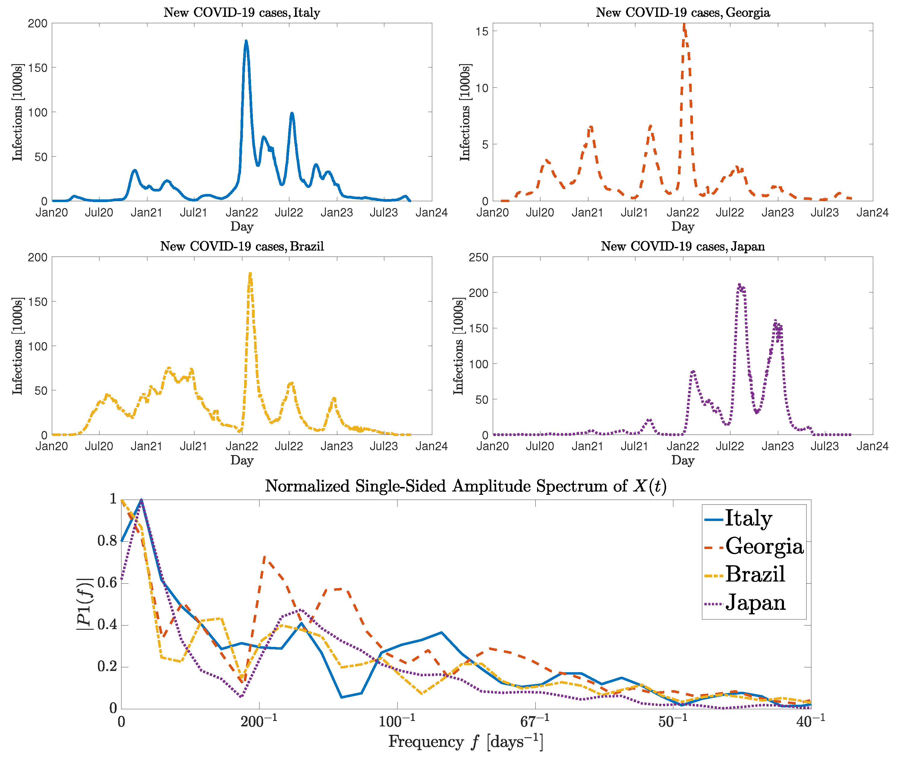
  1. Roser, M. Our World in Data. 2023. Available online: https://ourworldindata.org/coronavirus (accessed on 5 October 2023).
  2. Georgia Departent of Public Health. COVID19 Status Report. 2020. Available online: https://dph.georgia.gov/covid-19-status-report (accessed on 5 October 2023).
  3. Kermack, W.O.; McKendrick, A.G. A contribution to the mathematical theory of epidemics. Proc. R. Soc. Lond. Ser. A Contain. Pap. Math. Phys. Character 1927, 115, 700–721. [Google Scholar]
  4. Breda, D.; Diekmann, O.; De Graaf, W.; Pugliese, A.; Vermiglio, R. On the formulation of epidemic models (an appraisal of Kermack and McKendrick). J. Biol. Dyn. 2012, 6, 103–117. [Google Scholar] [CrossRef] [PubMed]
  5. Hethcote, H.W. The mathematics of infectious diseases. SIAM Rev. 2000, 42, 599–653. [Google Scholar] [CrossRef]
  6. Viguerie, A.; Lorenzo, G.; Auricchio, F.; Baroli, D.; Hughes, T.J.; Patton, A.; Reali, A.; Yankeelov, T.E.; Veneziani, A. Simulating the spread of COVID-19 via a spatially-resolved susceptible–exposed–infected–recovered–deceased (SEIRD) model with heterogeneous diffusion. Appl. Math. Lett. 2021, 111, 106617. [Google Scholar] [CrossRef]
  7. Grave, M.; Viguerie, A.; Barros, G.F.; Reali, A.; Coutinho, A.L. Assessing the spatio-temporal spread of COVID-19 via compartmental models with diffusion in Italy, USA, and Brazil. Arch. Comput. Methods Eng. 2021, 28, 4205–4223. [Google Scholar] [CrossRef]
  8. Zhang, S.; Ponce, J.; Zhang, Z.; Lin, G.; Karniadakis, G. An integrated framework for building trustworthy data-driven epidemiological models: Application to the COVID-19 outbreak in New York City. PLoS Comput. Biol. 2021, 17, e1009334. [Google Scholar] [CrossRef] [PubMed]
  9. Parolini, N.; Dede’, L.; Antonietti, P.F.; Ardenghi, G.; Manzoni, A.; Miglio, E.; Pugliese, A.; Verani, M.; Quarteroni, A. SUIHTER: A new mathematical model for COVID-19. Application to the analysis of the second epidemic outbreak in Italy. Proc. R. Soc. A 2021, 477, 20210027. [Google Scholar] [CrossRef]
  10. Bhouri, M.A.; Costabal, F.S.; Wang, H.; Linka, K.; Peirlinck, M.; Kuhl, E.; Perdikaris, P. COVID-19 dynamics across the US: A deep learning study of human mobility and social behavior. Comput. Methods Appl. Mech. Eng. 2021, 382, 113891. [Google Scholar] [CrossRef]
  11. Jardón-Kojakhmetov, H.; Kuehn, C.; Pugliese, A.; Sensi, M. A geometric analysis of the SIS, SIRS and SIRWS epidemiological models. Nonlinear Anal. Real World Appl. 2021, 58, 103220. [Google Scholar] [CrossRef]
  12. Anggriani, N.; Ndii, M.Z.; Amelia, R.; Suryaningrat, W.; Pratama, M.A.A. A mathematical COVID-19 model considering asymptomatic and symptomatic classes with waning immunity. Alex. Eng. J. 2022, 61, 113–124. [Google Scholar] [CrossRef]
  13. Crellen, T.; Pi, L.; Davis, E.L.; Pollington, T.M.; Lucas, T.C.; Ayabina, D.; Borlase, A.; Toor, J.; Prem, K.; Medley, G.F.; et al. Dynamics of SARS-CoV-2 with waning immunity in the UK population. Philos. Trans. R. Soc. B 2021, 376, 20200274. [Google Scholar] [CrossRef] [PubMed]
  14. Altmann, D.M.; Boyton, R.J. Waning immunity to SARS-CoV-2: Implications for vaccine booster strategies. Lancet Respir. Med. 2021, 9, 1356–1358. [Google Scholar] [CrossRef] [PubMed]
  15. Dolgin, E. COVID vaccine immunity is waning-how much does that matter. Nature 2021, 597, 606–607. [Google Scholar] [CrossRef] [PubMed]
  16. Dafilis, M.P.; Frascoli, F.; Wood, J.G.; McCaw, J.M. The influence of increasing life expectancy on the dynamics of SIRS systems with immune boosting. ANZIAM J. 2012, 54, 50–63. [Google Scholar] [CrossRef]
  17. Lavine, J.S.; King, A.A.; Bjørnstad, O.N. Natural immune boosting in pertussis dynamics and the potential for long-term vaccine failure. Proc. Natl. Acad. Sci. USA 2011, 108, 7259–7264. [Google Scholar] [CrossRef]
  18. Wang, G.; Xiang, Z.; Wang, W.; Chen, Z. Seasonal coronaviruses and SARS-CoV-2: Effects of preexisting immunity during the COVID-19 pandemic. J. Zhejiang Univ.-Sci. B 2022, 23, 451–460. [Google Scholar] [CrossRef]
  19. Fillmore, N.R.; Szalat, R.E.; La, J.; Branch-Elliman, W.; Monach, P.A.; Nguyen, V.; Samur, M.K.; Brophy, M.T.; Do, N.V.; Munshi, N.C. Recent common human coronavirus infection protects against severe acute respiratory syndrome coronavirus 2 (SARS-CoV-2) infection: A Veterans Affairs cohort study. Proc. Natl. Acad. Sci. USA 2022, 119, e2213783119. [Google Scholar] [CrossRef]
  20. Grifoni, A.; Weiskopf, D.; Ramirez, S.I.; Mateus, J.; Dan, J.M.; Moderbacher, C.R.; Rawlings, S.A.; Sutherland, A.; Premkumar, L.; Jadi, R.S.; et al. Targets of T cell responses to SARS-CoV-2 coronavirus in humans with COVID-19 disease and unexposed individuals. Cell 2020, 181, 1489–1501. [Google Scholar] [CrossRef]
  21. Edridge, A.W.; Kaczorowska, J.; Hoste, A.C.; Bakker, M.; Klein, M.; Loens, K.; Jebbink, M.F.; Matser, A.; Kinsella, C.M.; Rueda, P.; et al. Seasonal coronavirus protective immunity is short-lasting. Nat. Med. 2020, 26, 1691–1693. [Google Scholar] [CrossRef]
  22. van Boven, M.; de Melker, H.E.; Schellekens, J.F.; Kretzschmar, M. Waning immunity and sub-clinical infection in an epidemic model: Implications for pertussis in The Netherlands. Math. Biosci. 2000, 164, 161–182. [Google Scholar] [CrossRef]
  23. Laidlaw, B.J.; Ellebedy, A.H. The germinal centre B cell response to SARS-CoV-2. Nat. Rev. Immunol. 2022, 22, 7–18. [Google Scholar] [CrossRef] [PubMed]
  24. Paniskaki, K.; Anft, M.; Thieme, C.J.; Skrzypczyk, S.; Konik, M.J.; Dolff, S.; Westhoff, T.H.; Nienen, M.; Stittrich, A.; Stervbo, U.; et al. Severe acute respiratory syndrome coronavirus 2 cross-reactive b and T cell responses in kidney transplant patients. Transplant. Proc. 2022, 54, 1455–1464. [Google Scholar] [CrossRef] [PubMed]
  25. Yang, X.; Chen, L.; Chen, J. Permanence and positive periodic solution for the single-species nonautonomous delay diffusive models. Comput. Math. Appl. 1996, 32, 109–116. [Google Scholar] [CrossRef]
  26. Li, H.; Guo, S. Dynamics of a SIRC epidemiological model. Electron. J. Differ. Equ. 2017, 121, 1–18. [Google Scholar]
  27. Roy, A.K.; Roy, P.K. Treatment of psoriasis by interleukin-10 through impulsive control strategy: A mathematical study. In Mathematical Modelling, Optimization, Analytic and Numerical Solutions; Springer: Berlin/Heidelberg, Germany, 2020; pp. 313–332. [Google Scholar]
  28. Roy, A.K.; Nelson, M.; Roy, P.K. A control-based mathematical study on psoriasis dynamics with special emphasis on IL-21 and IFN-γ interaction network. Math. Methods Appl. Sci. 2021, 44, 13403–13420. [Google Scholar] [CrossRef]
  29. Roy, A.K.; Al Basir, F.; Roy, P.K.; Chatterjee, A.N. A model analysis to measure the adherence of Etanercept and Fezakinumab therapy for the treatment of psoriasis. Nonlinear Anal. Model. Control 2022, 27, 513–533. [Google Scholar] [CrossRef]
  30. Birkhoff, G.; Rota, G. Ordinary Differential Equations; John Wiley& Sons: Hoboken, NJ, USA, 1978. [Google Scholar]
  31. Hartman, P. Ordinary Differential Equations; SIAM: Philadelphia, PA, USA, 2002. [Google Scholar]
  32. MATLAB, version R2019b; The MathWorks Inc.: Natick, MA, USA, 2019.
Figure 1. Top: Infected population in Italy, Georgia (USA), Japan, and Brazil over the time range January 2020–September 2023. We observe clear oscillatory dynamics [1,2]. The data are smoothened with a 7-day moving average. Bottom: Fourier single-sided spectral analysis showing the dominant frequencies for the new infections in the same four countries/states.
Mathematics 11 04918 g001
Figure 2. Block diagram of the SIRW model. The red arrows refer to nonlinear dynamics (similar to a predator-prey model).
Mathematics 11 04918 g002
Figure 3. SIRW model: results with a limit cycle (top) and with a constant equilibrium (bottom), respective parameters given in Table 1. Top-right and bottom-right zoom the infected population at the beginning and the end of the simulation, showing the convergence to a periodic behavior (left) or stable equilibrium (right).
Mathematics 11 04918 g003
Figure 4. Block diagram of the SIRW2 model. Again, the red arrows refer to nonlinear dynamics (similar to a predator–prey model).
Mathematics 11 04918 g004
Figure 5. Simulation set 1: limit cycle. Synopsis of the compartments (top-left), i u and i e (top-right), total infected (bottom-left) and sensitivity of the infected on χ u u (bottom-right).
Mathematics 11 04918 g005
Figure 6. Simulation set 2: Non-disease-free equilibrium. Synopsis of the compartments (top-left), i u and i e (top-right), total infected (bottom-left) and w u and w e (bottom-right).
Mathematics 11 04918 g006
Figure 7. Simulation set 3: Disease-free equilibrium. Synopsis of the compartments (top-left), i u and i e (top-right), total infected (bottom-left) and w u and w e (bottom-right).
Mathematics 11 04918 g007
Figure 8. More realistic example: The SIRW2 model compared to data from Italy. Notably, COVID-19 mortality is well-captured, both qualitatively and quantitatively, and the timing of the different waves aligns with surveillance data.
Mathematics 11 04918 g008
Figure 9. More realistic example: The SIRW2 model compared to data from Brazil. Notably, COVID-19 mortality is well-captured, both qualitatively and quantitatively, and the timing of the different waves aligns with surveillance data.
Mathematics 11 04918 g009
Table 1. Relevant variables, parameters, parameter names, and units for the system (1).
Parameter/VariableNameUnitsPeriodicSteady Equilibrium
sSusceptible individualsPersons99999999
iInfected individualsPersons11
rRecovered individualsPersons00
wWaning-immunity individualsPersons00
β Contact rate between s and iPersons 1 · Days 1 5.5 × 10 5 5.5 × 10 5
ϕ Recovery rateDays 1 0.050.05
ξ Loss-of-immunity initiation rateDays 1 5 × 10 5 0.005
χ Immunity boosting-contact ratePersons 1 · Days 1 2 × 10 3 2 × 10 3
κ Loss-of-immunity rateDays 1 0.0050.005
Table 2. Relevant variables, parameters, parameter names, and units for the system (2).
Parameter/VariableNameUnits
s u , e Susceptible individuals (no prior immunity, prior immunity)Persons
i u , e Infected individuals (no prior immunity, prior immunity)Persons
r u , e Recovered individuals (no prior immunity, prior immunity)Persons
w u , e Waning-immunity individuals (no prior immunity, prior immunity)Persons
mDeceased individualsPersons
β u u , e , β e u , e Contact rate between s u and i u , i e , s e and i u , i e .Persons 1 · Days 1
ϕ u , e Recovery rate for i u , i e Days 1
ξ u , e Loss-of-immunity initiation rate for r u , r e Days 1
χ u u , e , χ e u , e Immunity boosting rates for r u , r e Persons 1 · Days 1
κ u , e Loss-of-immunity rate for w u , w e Days 1
γ u , e Mortality rate from disease, for i u , i e Days 1
α Vaccination rateDays 1
Π Recruitment ratePersons · Days 1
ρ General mortality rateDays 1
Table 3. Parameter values for the shown simulations.
Parameter/VariableUnitsSim1Sim2Sim3
s u 0 , e 0 Persons9999, 09999, 09999, 0
i u 0 , e 0 Persons30, 030, 030, 0
r u 0 , e 0 Persons0, 00, 00, 0
w u 0 , e 0 Persons0, 00, 00, 0
mPersons000
β u u , e Persons 1 · Days 1 1.54 ×   10 5 , 4 ×   10 5 1.54 ×   10 5 , 4 ×   10 5 1.54 ×   10 5 , 4 ×   10 5
β e u , e Persons 1 · Days 1 5.5 ×   10 5 , 5.5 ×   10 5 5.5 ×   10 5 , 5.5 ×   10 5 5.5 ×   10 5 , 5.5 ×   10 5
ϕ u , e Days 1 0.13, 0.140.13, 0.140.13, 0.28
ξ u , e Days 1 0.005, 0.0050.005, 0.0050.05, 0.005
χ u u , e Persons 1 · Days 1 7.7 ×   10 5 , 3.0 ×   10 3 7.7 ×   10 5 , 3.0 ×   10 3 7.7 ×   10 5 , 3.0 ×   10 3
χ e u , e Persons 1 · Days 1 2.8 ×   10 4 , 2.8 ×   10 4 2.8 ×   10 4 , 2.8 ×   10 4 2.8 ×   10 4 , 2.8 ×   10 4
κ u , e Days 1 0.005, 0.0050.005, 0.0050.05, 0.005
γ u , e Days 1 0.003, 4.4 ×   10 5 0.003, 4.4 ×   10 5 0.0, 0.0
α Days 1 0.0020.0040.0022
ψ Days 1 5 ×   10 5 5 ×   10 5 5 ×   10 5
ρ Days 1 5 ×   10 5 5 ×   10 5 5 ×   10 5
Table 4. Parameter values for the shown simulation.
Parameter/VariableUnitsItaly-Inspired CaseBrazil-Inspired Case
s u 0 , e 0 Persons59,000,000, 0214,000,000, 0
i u 0 , e 0 Persons176,488, 0400,488, 0
r u 0 , e 0 Persons0, 00, 0
w u 0 , e 0 Persons0, 00, 0
mPersons00
β u u , e Persons 1 · Days 1 1.9 ×   10 9 , 3.4 ×   10 9 1.9 ×   10 9 , 3.4 ×   10 9
β e u , e Persons 1 · Days 1 1.1 ×   10 8 , 1.1 ×   10 8 1.1 ×   10 8 , 1.1 ×   10 8
ϕ u , e Days 1 0.11, 0.110.11, 0.11
ξ u , e Days 1 0.01, 0.010.01, 0.01
χ u u , e Persons 1 · Days 1 1.3 ×   10 8 , 5.1 ×   10 8 1.3 ×   10 8 , 5.1 ×   10 8
χ e u , e Persons 1 · Days 1 1.3 ×   10 8 , 4.7 ×   10 8 1.3 ×   10 8 , 4.7 ×   10 8
κ u , e Days 1 0.0083, 0.00830.0083, 0.0083
γ u , e Days 1 0.002, 0.00010.003, 0.00015
α Days 1 0.0050.005
ψ Days 1 3 ×   10 5 3 ×   10 5
ρ Days 1 2.9 ×   10 5 2.9 ×   10 5
Disclaimer/Publisher’s Note: The statements, opinions and data contained in all publications are solely those of the individual author(s) and contributor(s) and not of MDPI and/or the editor(s). MDPI and/or the editor(s) disclaim responsibility for any injury to people or property resulting from any ideas, methods, instructions or products referred to in the content.

