
The Enhanced Wagner–Hagras OLS–BP Hybrid Algorithm for Training IT3 NSFLS-1 for Temperature Prediction in HSM Processes

 ,
, 
 , and
, and 
Abstract
:1. Introduction
- The detailed and novel mathematical formulation of the novel hybrid OLS–BP training algorithm applied to the novel EWH IT3 NSFLS-1 fuzzy logic systems.
- A more precise, economical, and novel method to estimate the final value of the IT3 fuzzy logic systems.
- Using a novel method to construct the EWH IT3 NSFLS-1 system with a dynamical structure.
- To the authors’ best knowledge, this is the first time that a hybrid EWH IT3 NSFLS-1 (OLS–BP) fuzzy system is applied to predict the transfer bar surface temperature at the entry zone of the finishing scale breaker of an HSM.
2. Materials and Methods
2.1. A New Construction and Calculation of the WH IT3 NSFLS-1 System
2.1.1. Input Variables, Rules, and Levels-
2.1.2. The Membership Functions and UOD
2.1.3. The Rule Base
2.1.4. Alpha -Cuts
2.1.5. Firing Intervals
2.1.6. Consequent Centroids
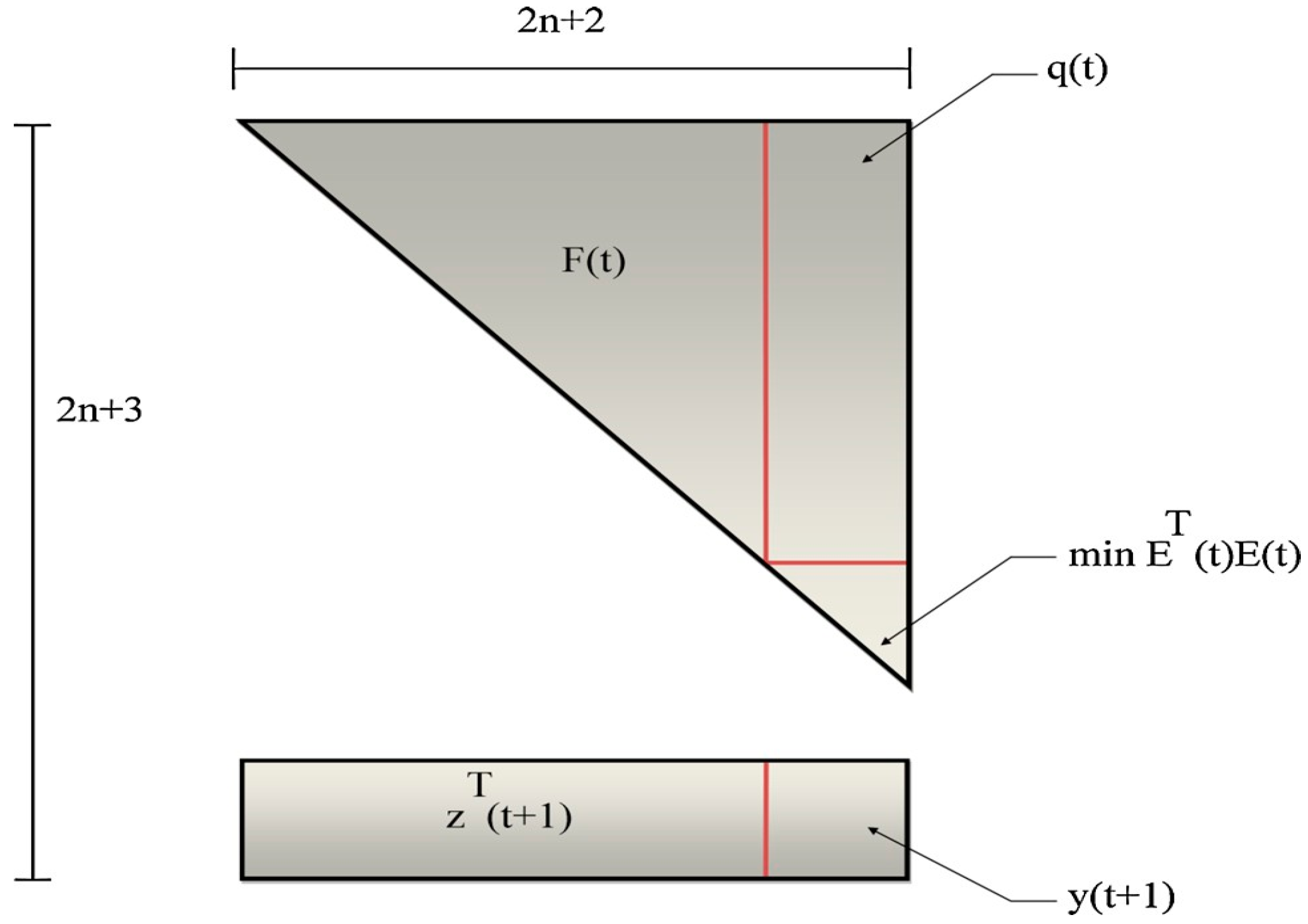
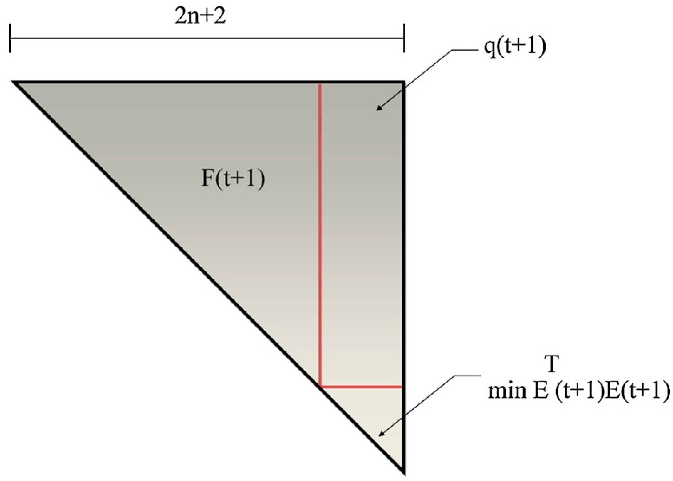
2.1.7. Expansion of the Level-
2.1.8. Calculation of
2.2. The Backpropagation Method for Antecedent Tuning
2.3. The OLS Method for Consequent Tuning
| Algorithm 1: Parameter estimation using rotational orthogonal transformation | |
| 1: | Initialize , , , , and |
| 2: | Triangulate matrices |
| 3: | Solve |
| 4: | Assign estimated values. , |
2.4. The Convergence Analysis
3. Results and Discussion
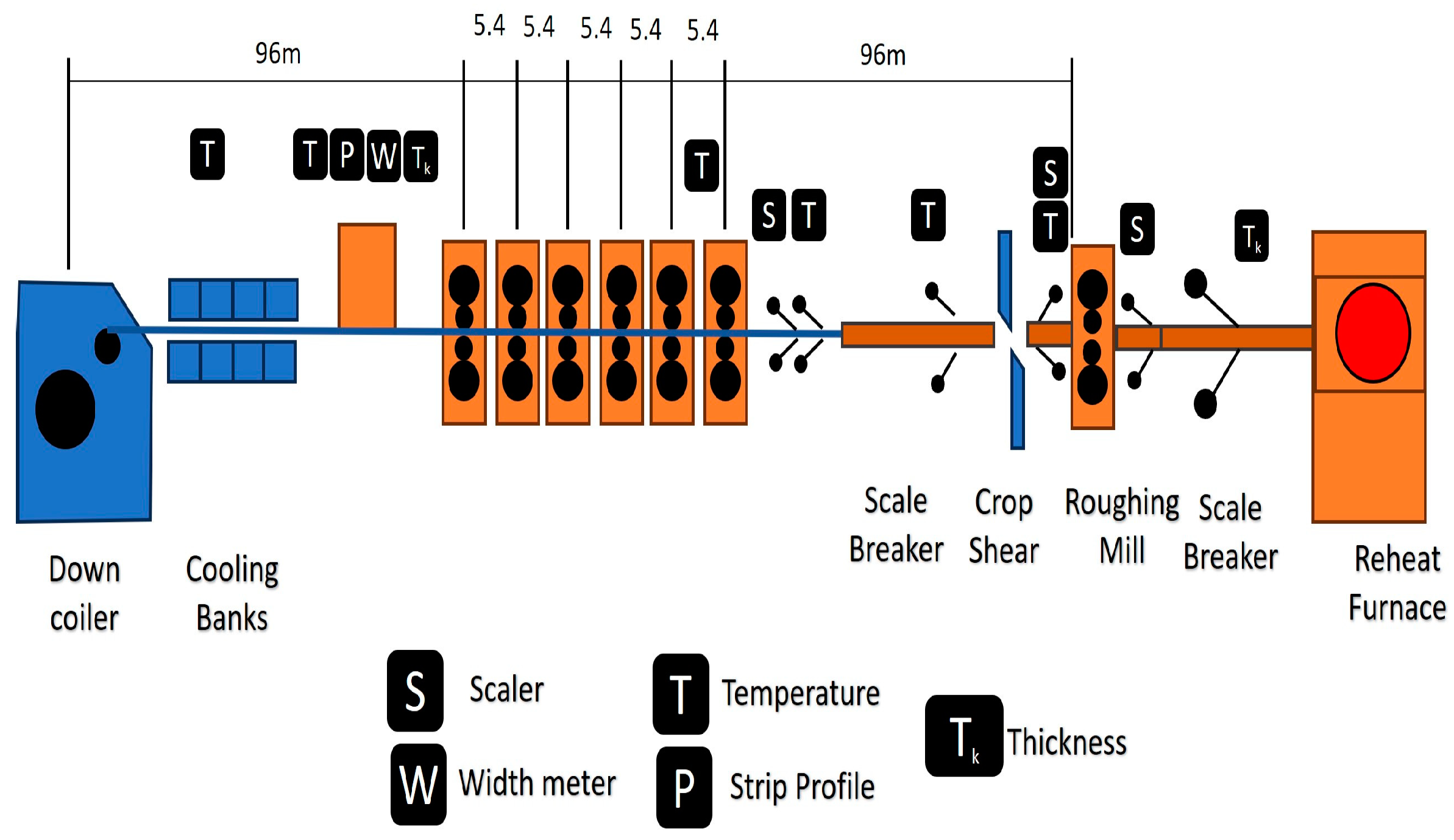
3.1. The Problem: Industrial Process Description
3.2. Simulation
3.2.1. Input–Output Data Pairs
3.2.2. Antecedent Membership Functions
3.2.3. Fuzzy Rule Base
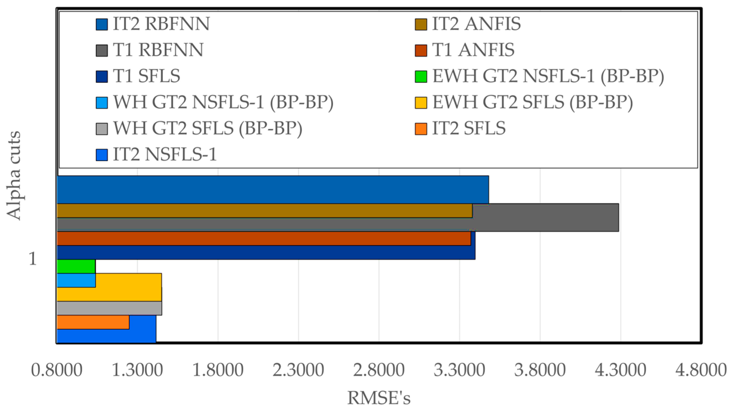
3.3. Results and Discussion
4. Conclusions
Author Contributions
Funding
Data Availability Statement
Conflicts of Interest
Abbreviations
| FLS | Fuzzy logic systems. |
| MF | Membership function. |
| SFLS | Singleton fuzzy logic systems. |
| NS-1 | Type-1 non-singleton. |
| NS-2 | Type-2 non-singleton. |
| NSFLS-1 | Type-1 non-singleton fuzzy logic systems. |
| NSFLS-2 | Type-2 non-singleton fuzzy logic systems. |
| T1 | Type-1. |
| T2 | Type-2. |
| ANFIS | Adaptive network fuzzy inference systems. |
| RBFNN | Radial basis function neural networks. |
| IT2 | Interval type-2. |
| GT2 | General type-2. |
| IT3 | Interval type-3. |
| BP | Back-propagation. |
| OLS | Orthogonal least square. |
| WH | Wagner–Hagras. |
| EWH | Enhanced Wagner–Hagras. |
| RM | Roughing mill. |
| FM | Finishing mill. |
| SB | Scale breaker. |
| CLR | Coiler. |
| HSM | Hot strip mill. |
| MC | Maximum correntropy. |
| KF | Kalman filter. |
| CKF | Correntropy Kalman filter. |
| ARV’s | Automated remote vehicles. |
| PID | Proportional, integral, and derivative. |
| TSK | Takagi–Sugeno–Kang. |
| OWA | Ordered weighted averaging. |
| ANN | Artificial neural network. |
| RLS | Recursive least squares. |
| PSO | Particle swam optimization. |
| BBO | Biogeography-based optimization. |
| LSE | Least square estimator |
| TLBO | Teaching learning-based optimization. |
| KRR | Kernel ridge regression. |
| SVM | Support vector machine. |
| GD | Gradient descent. |
| RBM | Boltzmann machine. |
| Parate | Pitch adjustment rate. |
| HS | Harmony search. |
| AE | Approximate error. |
| DRL | Deep reinforcement learning. |
| UKF | Unscented Kalman filter. |
| SGLOS | Surge-guided line-of-sight. |
| WLS | Weighted least square. |
| NMPC | Nonlinear model predictive control. |
| MPPT | Maximum power point tracking. |
| MOAHA | Multi-objective artificial hummingbird algorithm. |
| EKF | Enhanced Kalman filter. |
Appendix A


References
- Castillo, O.; Castro, J.R.; Melin, P. Interval type-3 fuzzy fractal approach in sound speaker quality control evaluation. Eng. Appl. Artif. Intell. 2022, 116, 105363. [Google Scholar] [CrossRef]
- Castillo, O.; Castro, J.R.; Melin, P. Interval Type-3 Fuzzy Systems: Theory and Design, 1st ed.; Studies in Fuzziness and Soft Computing; Springer Nature: Cham, Switzerland, 2022; Volume 418, pp. 1–100. [Google Scholar] [CrossRef]
- Castillo, O.; Melin, P. Towards interval type-3 intuitionistic fuzzy sets and systems. Mathematics 2022, 10, 4091. [Google Scholar] [CrossRef]
- Peraza, C.; Ochoa, P.; Castillo, O.; Geem, Z.W. Interval type-3 fuzzy differential evolution for designing an interval type-3 fuzzy controller of a unicycle mobile robot. Mathematics 2022, 10, 3533. [Google Scholar] [CrossRef]
- Méndez, G.M.; Lopez-Juarez, I.; Dorantes, P.N.M.; Alcorta, M.A. A New method for design of interval type-3 fuzzy logic systems with uncertain type-2 non-singleton inputs (IT3 NSFLS-2): A study case in a hot strip mill. IEEE Access 2023, 11, 44065–44081. [Google Scholar] [CrossRef]
- Amador-Angulo, L.; Castillo, O.; Melin, P.; Castro, J.R. Interval type-3 fuzzy adaptation of the bee colony optimization algorithm for optimal fuzzy control of an autonomous mobile robot. Micromachines 2022, 13, 1490. [Google Scholar] [CrossRef] [PubMed]
- Castillo, O.; Castro, J.R.; Melin, P. Interval type-3 fuzzy control for automated tuning of image quality in televisions. Axioms 2022, 11, 276. [Google Scholar] [CrossRef]
- Castillo, O.; Castro, J.R.; Melin, P. Forecasting the COVID-19 with interval type-3 fuzzy logic and the fractal dimension. Int. J. Fuzzy Syst. 2022, 25, 182–197. [Google Scholar] [CrossRef]
- Castillo, O.; Castro, J.R.; Melin, P. A methodology for building interval type-3 fuzzy systems based on the principle of justifiable granularity. Int. J. Intell. Syst. 2022, 37, 7909–7943. [Google Scholar] [CrossRef]
- Castillo, O.; Pulido, M.; Melin, P. Interval Type-3 Fuzzy Aggregators for Ensembles of Neural Networks in Time Series Prediction. In Proceedings of the International Conference on Intelligent and Fuzzy Systems, Izmir, Turkey, 19–21 July 2022; Springer: Cham, Switzerland; pp. 785–793. [Google Scholar] [CrossRef]
- Castillo, O.; Castro, J.R.; Melin, P. Interval type-3 fuzzy aggregation of neural networks for multiple time series prediction: The case of financial forecasting. Axioms 2022, 11, 6. [Google Scholar] [CrossRef]
- Castillo, O.; Castro, J.R.; Pulido, M.; Melin, P. Interval type-3 fuzzy aggregators for ensembles of neural networks in COVID-19 time series prediction. Eng. Appl. Artif. Intell. 2022, 114, 105–110. [Google Scholar] [CrossRef]
- Mohammadzadeh, A.; Castillo, O.; Band, S.S.; Mosavi, A. A novel fractional-order multiple-model type-3 fuzzy control for nonlinear systems with unmodeled dynamics. Int. J. Fuzzy Syst. 2021, 23, 1633–1651. [Google Scholar] [CrossRef]
- Aly, A.A.; Felemban, B.F.; Mohammadzadeh, V.; Castillo, O.; Bartoszewicz, A. Frequency regulation system: A deep learning identification, type-3 fuzzy control and LMI stability analysis. Energies 2021, 14, 7801. [Google Scholar] [CrossRef]
- Castillo, O.; Valdez, F.; Peraza, C.; Yoon, J.H.; Geem, Z.W. High-speed interval type-2 fuzzy systems for dynamic parameter adaptation in harmony search for optimal design of fuzzy controllers. Mathematics 2021, 9, 758. [Google Scholar] [CrossRef]
- Melin, P.; Sánchez, D.; Castro, J.R.; Castillo, O. Design of type-3 fuzzy systems and ensemble neural networks for COVID-19 time series prediction using a firefly algorithm. Axioms 2022, 11, 410. [Google Scholar] [CrossRef]
- Kreinovich, V.; Kosheleva, O.; Melin, P.; Castillo, O. Efficient algorithms for data processing under type-3 (and higher) fuzzy uncertainty. Mathematics 2022, 10, 2361. [Google Scholar] [CrossRef]
- Liu, Z.; Mohammadzadeh, A.; Turabieh, H.; Mafarja, M.; Band, S.; Mosavi, A. A new online learned interval type-3 fuzzy control system for solar energy management systems. IEEE Access 2021, 9, 10498–10508. [Google Scholar] [CrossRef]
- Mohammadzadeh, A.; Sabzalian, M.H.; Zhang, W. An interval type-3 fuzzy system and a new online fractional-order learning algorithm: Theory and practice. IEEE T. Fuzzy Syst. 2019, 28, 1940–1950. [Google Scholar] [CrossRef]
- Tian, M.W.; Yan, S.R.; Mohammadzadeh, A.; Tavoosi, J.; Mobayen, S.; Safdar, R.; Assawinchaichote, W.; Vu, M.A.; Zhilenkov, A. Stability of interval type-3 fuzzy controllers for autonomous vehicles. Mathematics 2021, 9, 2742. [Google Scholar] [CrossRef]
- Taghieh, A.; Mohammadzadeh, C.; Zhang, S.; Rathinasamy; Bekiros, S. A novel adaptive interval type-3 neuro-fuzzy robust controller for nonlinear complex dynamical systems with inherent uncertainties. Nonlinear Dyn. 2022, 111, 411–425. [Google Scholar] [CrossRef]
- Singh, D.J.; Verma, N.K.; Ghosh, A.K.; Malagaudanavar, A. An approach towards the design of interval type-3 T-S fuzzy system. IEEE Trans. Fuzzy Syst. 2022, 30, 3880–3893. [Google Scholar] [CrossRef]
- Gheisarnejad, M.; Mohammadzadeh, A.; Khooban, M.H. Model predictive control-based type-3 fuzzy estimator for voltage stabilization of DC power converters. IEEE Trans. Ind. Electron. 2021, 69, 13849–13858. [Google Scholar] [CrossRef]
- Qasem, S.N.; Ahmadian, A.; Mohammadzadeh, A.; Rathinasamy, S.; Pahlevanzadeh, B. A type-3 logic fuzzy system: Optimized by a correntropy based Kalman filter with adaptive fuzzy kernel size. Inf. Sci. 2021, 572, 424–443. [Google Scholar] [CrossRef]
- Gheisarnejad, M.; Mohammadzadeh, A.; Farsizadeh, V.; Khooban, M.H. Stabilization of 5G telecom converter-based deep type-3 fuzzy machine learning control for telecom applications. IEEE Trans. Circuits-II 2021, 69, 544–548. [Google Scholar] [CrossRef]
- Taghieh, A.; Mohammadzadeh, A.; Zhang, C.; Kausar, N.; Castillo, O. A type-3 fuzzy control for current sharing and voltage balancing in microgrids. Appl. Soft Comput. 2022, 129, 109636. [Google Scholar] [CrossRef]
- Taghieh, A.; Zhang, C.; Alattas, K.A.; Bouteraa, Y.; Rathinasamy, S.; Mohammadzadeh, A. A predictive type-3 fuzzy control for underactuated surface vehicles. Ocean Eng. 2022, 266, 11301. [Google Scholar] [CrossRef]
- Wang, J.H.; Tavoosi, J.; Mohammadzadeh, A.; Mobayen, S.; Asad, J.H.; Assawinchaichote, W.; Vu, M.T.; Skruch, P. Non-Singleton type-3 fuzzy approach for flowmeter fault detection, experimental study in a gas industry. Sensors 2021, 21, 7419. [Google Scholar] [CrossRef] [PubMed]
- Balootaki, M.A.; Rahmani, H.; Moeinkhah, H.; Mohammadzadeh, A. Non-singleton fuzzy control for multisynchronization of chaotic systems. Appl. Soft Comput. 2020, 99, 106924. [Google Scholar] [CrossRef]
- Alattas, K.A.; Mohammadzadeh, A.; Mobayen, S.; Aly, A.A.; Felemban, B.F. A new data-driven control system for MEMSs gyroscopes: Dynamics estimation by type-3 fuzzy systems. Micromachines 2021, 12, 1390. [Google Scholar] [CrossRef]
- Mosavi, A.; Shokri, S.N.; Qasem, M.; Band, S.S.; Mohammadzadeh, A. Fractional-order fuzzy control approach for photovoltaic/battery systems under unknown dynamics, variable irradiation and temperature. Electronics 2020, 9, 1455. [Google Scholar] [CrossRef]
- Tian, M.W.; Mohammadzadeh, A.; Tavoosi, J.; Mobayen, S.; Asad, J.H.; Castillo, O.; Várkonyi-Kóczy, A.R. A deep-learned type-3 fuzzy system and its application in modeling problems. Acta Polytech. Hung. 2022, 19, 151–172. [Google Scholar] [CrossRef]
- Tian, M.W.; Bouteraa, Y.; Alattas, K.A.; Yan, S.R.; Alanazi, A.K.; Mohammadzadeh, A.; Mobayen, S. A type-3 fuzzy approach for stabilization and synchronization of chaotic systems: Applicable for financial and physical chaotic systems. Complexity 2022, 2022, 8437910. [Google Scholar] [CrossRef]
- Mohammadzadeh, A.; Vafaie, R.H. A deep learned fuzzy control for inertial sensing: Micro electromechanical systems. Appl. Soft Comput. 2021, 109, 107597. [Google Scholar] [CrossRef]
- Nabipour, N.; Qasem, S.N.; Jermsittiparsert, K. Type-3 fuzzy voltage management in PV/hydrogen fuel cell/battery hybrid systems. Int. J. Hydrogen Energy 2020, 45, 32478–32492. [Google Scholar] [CrossRef]
- Hua, G.; Wang, F.; Zhang, J.; Alattas, K.A.; Mohammadzadeh, A.; The Vu, M. A new type-3 fuzzy predictive approach for mobile robots. Mathematics 2021, 10, 3186. [Google Scholar] [CrossRef]
- Yan, S.; Aly, A.A.; Felemban, B.F.; Gheisarnejad, M.; Tian, M.; Khooban, M.H.; Mohammadzadeh, A.; Mobayen, S. A new event-triggered type-3 fuzzy control system for multi-agent systems: Optimal economic efficient approach for actuator activating. Electronics 2021, 10, 3122. [Google Scholar] [CrossRef]
- Cao, Y.; Raise, A.; Mohammadzadeh, A.; Rathinasamy, S.; Band, S.S.; Mosavi, A. Deep learned recurrent type-3 fuzzy system: Applications for renewable energy modeling/prediction. Energy Rep. 2021, 7, 8115–8127. [Google Scholar] [CrossRef]
- Ma, C.; Mohammadzadeh, A.; Turabieh, H.; Mafarja, M.; Band, S.S.; Mosavi, A. Optimal type-3 fuzzy system for solving singular multi-pantograph Equations. IEEE Access 2020, 8, 225692–225702. [Google Scholar] [CrossRef]
- Vafaie, R.H.; Mohammadzadeh, A.; Piran, M.J. A new type-3 fuzzy predictive controller for mems gyroscopes. Nonlinear Dynam. 2021, 106, 381–403. [Google Scholar] [CrossRef]
- Montes-Dorantes, P.N.; Méndez, G.M. Non-Iterative Wagner-Hagras General type-2 Mamdani Singleton Fuzzy logic System Optimized by Central Composite Design in Quality Assurance by Image Processing. In Recent trends on Type-2 Fuzzy Logic Systems: Theory, Methodology and Applications; Castillo, O., Kumar, A., Eds.; Studies in Fuzziness and Soft Computing; Springer: Cham, Switzerland, 2023; Volume 425. [Google Scholar] [CrossRef]
- Melin, P.; Castillo, O. An intelligent hybrid approach for industrial quality control combining neural networks, fuzzy logic, and fractal theory. Inf. Sci. 2007, 177, 1543–1557. [Google Scholar] [CrossRef]
- Gilan, S.S.; Sebt, M.H.; Shahhosseini, V. Computing with words for hierarchical competency-based selection of personnel in construction companies. Appl. Soft Comput. 2012, 12, 860–871. [Google Scholar] [CrossRef]
- Shahparast, H.; Mansoori, E.G. Developing an online general type-2 fuzzy classifier using evolving type-1 rules. Int. J. Approx. Reason. 2019, 113, 336–353. [Google Scholar] [CrossRef]
- Cheng-Dong, L.I.; Gui-Qing, Z.; Hui-Dong, W.; Wei-Na, R. Properties and data-driven design of perceptual reasoning method based linguistic dynamic systems. Acta Autom. Sin. 2014, 40, 2221–2232. [Google Scholar]
- Mittal, K.; Jain, A.; Vaisla, K.S.; Castillo, O.; Kacprzyk, J. A comprehensive review on type 2 fuzzy logic applications: Past, present and future. Eng. Appl. Artif. Intell. 2020, 95, 103916. [Google Scholar] [CrossRef]
- Ibrahim, A.A.; Zhou, H.B.; Tan, S.X.; Zhang, C.L.; Duan, J.A. Regulated Kalman filter based training of an interval type-2 fuzzy system and its evaluation. Eng. Appl. Artif. Intell. 2020, 95, 103867. [Google Scholar] [CrossRef]
- Balootaki, M.A.; Rahmani, H.; Moeinkhah, H.; Mohammadzadeh, A. On the synchronization and stabilization of fractional-order chaotic systems: Recent advances and future perspectives. Phys. A Stat. Mech. Its Appl. 2020, 551, 124203. [Google Scholar] [CrossRef]
- Ontiveros, E.; Melin, P.; Castillo, O. High order α-planes integration: A new approach to computational cost reduction of General Type-2 Fuzzy Systems. Eng. Appl. Artif. Intell. 2018, 4, 186–197. [Google Scholar] [CrossRef]
- Wu, D.; Mendel, J.M. Recommendations on designing practical interval type-2 fuzzy systems. Eng. Appl. Artif. Intell. 2019, 85, 182–193. [Google Scholar] [CrossRef]
- Chiclana, F.; Zhou, S.M. Type-reduction of general type-2 fuzzy sets: The type-1 OWA approach. Int. J. Intell. Syst. 2013, 28, 505–522. [Google Scholar] [CrossRef]
- Jeng, W.H.R.; Yeh, C.Y.; Lee, S.J. General Type-2 Fuzzy Neural Network with Hybrid Learning for Function Approximation. In Proceedings of the 2009 IEEE International Conference on Fuzzy Systems, Jeju, Republic of Korea, 20–24 August 2009; pp. 1534–1539. [Google Scholar]
- Figueroa-García, J.C.; Román-Flores, H.; Chalco-Cano, Y. Type–reduction of interval type–2 fuzzy numbers via the Chebyshev inequality. Fuzzy Sets Syst. 2022, 435, 164–180. [Google Scholar] [CrossRef]
- Yu, Q.; Dian, S.; Li, Y.; Liu, J.; Zhao, T. Similarity-based non-singleton general type-2 fuzzy logic controller with applications to mobile two-wheeled robots. J. Intell. Fuzzy Syst. 2019, 37, 6841–6854. [Google Scholar] [CrossRef]
- Zhao, T.; Yu, Q.; Dian, S.; Guo, R.; Li, S. Non-singleton general type-2 fuzzy control for a two-wheeled self-balancing robot. Int. J. Fuzzy Syst. 2019, 21, 1724–1737. [Google Scholar] [CrossRef]
- Chen, Y.; Wang, D. Forecasting by general type-2 fuzzy logic systems optimized with QPSO algorithms. Int. J. Control Autom. Syst. 2017, 15, 2950–2958. [Google Scholar] [CrossRef]
- Li, X.; Chen, Y. Discrete non-iterative centroid type-reduction algorithms on general type-2 fuzzy logic systems. Int. J. Fuzzy Syst. 2021, 23, 704–715. [Google Scholar] [CrossRef]
- Zhao, T.; Liu, J.; Dian, S.; Guo, R.; Li, S. Sliding-mode-control-theory-based adaptive general type-2 fuzzy neural network control for power-line inspection robots. Neurocomputing 2020, 401, 281–294. [Google Scholar] [CrossRef]
- Mai, D.S.; Dang, T.H.; Ngo, L.T. Optimization of interval type-2 fuzzy system using the PSO technique for predictive problems. J. Inf. Telecommun. 2021, 5, 197–213. [Google Scholar] [CrossRef]
- Mohammadzadeh, A.; Kumbasar, T. A new fractional-order general type-2 fuzzy predictive control system and its application for glucose level regulation. Appl. Soft Comput. 2020, 91, 106241. [Google Scholar] [CrossRef]
- Mohammadzadeh, A.; Ghaemi, S.; Kaynak, O.; Khanmohammadi, S. Observer-based method for synchronization of uncertain fractional order chaotic systems by the use of a general type-2 fuzzy system. Appl. Soft Comput. 2016, 49, 544–560. [Google Scholar] [CrossRef]
- Geramian, A.; Abraham, A. Customer classification: A mamdani fuzzy inference system standpoint for modifying the failure mode and effect analysis based three-dimensional approach. Expert Syst. Appl. 2021, 186, 115753. [Google Scholar] [CrossRef]
- Tavana, M.R.; Khooban, M.H.; Niknam, T. Adaptive PI controller to voltage regulation in power systems: STATCOM as a case study. ISA Trans. 2017, 66, 325–334. [Google Scholar] [CrossRef]
- Mohammadzadeh, A.; Sabzalian, M.H.; Ahmadian, A.; Nabipour, N. A dynamic general type-2 fuzzy system with optimized secondary membership for online frequency regulation. ISA Trans. 2021, 112, 150–160. [Google Scholar] [CrossRef]
- Torshizi, A.D.; Zarandi, M.H.F. A new cluster validity measure based on general type-2 fuzzy sets: Application in gene expression data clustering. Knowl. Based Syst. 2014, 64, 81–93. [Google Scholar] [CrossRef]
- Khooban, M.H.; Vafamand, N.; Liaghat, A.; Dragicevic, T. An optimal general type-2 fuzzy controller for urban traffic network. ISA Trans. 2017, 66, 335–343. [Google Scholar] [CrossRef] [PubMed]
- Mohammadzadeh, A.; Kaynak, O. A novel general type-2 fuzzy controller for fractional-order multi-agent systems under unknown time-varying topology. J. Frankl. Inst. 2019, 356, 5151–5171. [Google Scholar] [CrossRef]
- Ontiveros, E.; Melin, P.; Castillo, O. Comparative study of interval type-2 and general type-2 fuzzy systems in medical diagnosis. Inf. Sci. 2020, 525, 37–53. [Google Scholar] [CrossRef]
- Zarandi, M.F.; Soltanzadeh, S.; Mohammadi, A.; Castillo, O. Designing a general type-2 fuzzy expert system for diagnosis of depression. Appl. Soft Comput. 2019, 80, 329–341. [Google Scholar] [CrossRef]
- Salehi, F.; Keyvanpour, M.R.; Sharifi, A. GT2-CFC: General type-2 collaborative fuzzy clustering method. Inf. Sci. 2021, 578, 297–322. [Google Scholar] [CrossRef]
- Almaraashi, M.; John, R.; Hopgood, A.; Ahmadi, S. Learning of interval and general type-2 fuzzy logic systems using simulated annealing: Theory and practice. Inf. Sci. 2016, 360, 21–42. [Google Scholar] [CrossRef]
- Carvajal, O.; Melin, P.; Miramontes, I.; Prado-Arechiga, G. Optimal design of a general type-2 fuzzy classifier for the pulse level and its hardware implementation. Eng. Appl. Artif. Intell. 2021, 97, 104069. [Google Scholar] [CrossRef]
- Ontiveros-Robles, E.; Castillo, O.; Melin, P. Towards asymmetric uncertainty modeling in designing general type-2 fuzzy classifiers for medical diagnosis. Expert Syst. Appl. 2021, 183, 115370. [Google Scholar] [CrossRef]
- Doctor, F.; Syue, C.H.; Liu, Y.X.; Shieh, J.S.; Iqbal, R. Type-2 fuzzy sets applied to multivariable self-organizing fuzzy logic controllers for regulating anesthesia. Appl. Soft Comput. 2016, 38, 872–889. [Google Scholar] [CrossRef]
- Castillo, O.; Muhuri, P.K.; Melin, P.; Pulkkinen, P. Emerging issues and applications of type-2 fuzzy sets and systems. Eng. Appl. Artif. Intell. 2020, 90, 103596. [Google Scholar] [CrossRef]
- Sahab, N.; Hagras, H. Adaptive non-singleton type-2 fuzzy logic systems: A way forward for handling numerical uncertainties in real world applications. Int. J. Comput. Commun. Control 2011, 6, 503–529. [Google Scholar] [CrossRef]
- Ontiveros-Robles, E.; Melin, P. A hybrid design of shadowed type-2 fuzzy inference systems applied in diagnosis problems. Eng. Appl. Artif. Intell. 2019, 86, 43–55. [Google Scholar] [CrossRef]
- Ochoa, P.; Castillo, O.; Melin, P.; Soria, J. Differential evolution with shadowed and general type-2 fuzzy systems for dynamic parameter adaptation in optimal design of fuzzy controllers. Axioms 2021, 10, 194. [Google Scholar] [CrossRef]
- Wagner, C.; Hagras, H. Toward general type-2 fuzzy logic systems based on zSlices. IEEE Trans. Fuzzy Syst. 2010, 18, 637–660. [Google Scholar] [CrossRef]
- Shi, J.; Song, Y. Mathematical analysis of a simplified general type-2 fuzzy PID controller. Math. Biosci. Eng. 2020, 17, 7994–8036. [Google Scholar] [CrossRef] [PubMed]
- Ontiveros-Robles, E.; Melin, P.; Castillo, O. An efficient high-order α-plane aggregation in general type-2 fuzzy systems using newton–cotes rules. Int. J. Fuzzy Syst. 2021, 23, 1102–1121. [Google Scholar] [CrossRef]
- Melin, P.; Ontiveros-Robles, E.; Castillo, O. New Medical Diagnosis Models Based on Generalized Type-2 Fuzzy Logic, 1st ed.; Springer International Publishing: Cham, Switzerland, 2021. [Google Scholar] [CrossRef]
- Chen, Y.; Li, C.; Yang, J. Design and application of Nagar-Bardini structure-based interval type-2 fuzzy logic systems optimized with the combination of backpropagation algorithms and recursive least square algorithms. Expert Syst. Appl. 2023, 211, 118596. [Google Scholar] [CrossRef]
- El-Nagar, A.M.; El-Bardini, M.; Khater, A.A. A class of general type-2 fuzzy controller based on adaptive alpha-plane for nonlinear systems. Appl. Soft Comput. 2023, 133, 109938. [Google Scholar] [CrossRef]
- Hazarika, B.B.; Gupta, D. Affinity based fuzzy kernel ridge regression classifier for binary class imbalance learning. Eng. Appl. Artif. Intell. 2023, 117, 105544. [Google Scholar] [CrossRef]
- Yin, R.; Pan, X.; Zhang, L.; Yang, J.; Lu, W. A rule-based deep fuzzy system with nonlinear fuzzy feature transform for data classification. Inf. Sci. 2023, 633, 431–452. [Google Scholar] [CrossRef]
- Sabahi, K.; Zhang, C.; Kausar, N.; Mohammadzadeh, A.; Pamucar, D.; Mosavi, A.H. Input-output scaling factors tuning of type-2 fuzzy PID controller using multi-objective optimization technique. AIMS Math. 2022, 8, 7917–7932. [Google Scholar] [CrossRef]
- Sedaghati, A.; Pariz, N.; Siahi, M.; Barzamini, R. A new adaptive non-singleton general type-2 fuzzy control of induction motors subject to unknown time-varying dynamics and unknown load torque. Soft Comput. 2021, 25, 5895–5907. [Google Scholar] [CrossRef]
- Sabzalian, M.H.; Mohammadzadeh, A.; Rathinasamy, S.; Zhang, W. A developed observer-based type-2 fuzzy control for chaotic systems. Int. J. Syst. Sci. 2021, 54, 2921–2940. [Google Scholar] [CrossRef]
- Huang, H.; Xu, H.; Chen, F.; Zhang, C.; Mohammadzadeh, A. An applied type-3 fuzzy logic system: Practical matlab simulink and M-files for robotic, control, and modeling applications. Symmetry 2023, 15, 475. [Google Scholar] [CrossRef]
- Mehrmolaei, S.; Savargiv, M.; Keyvanpour, M.R. Hybrid learning-oriented approaches for predicting Covid-19 time series data: A comparative analytical study. Eng. Appl. Artif. Intell. 2023, 126, 106754. [Google Scholar] [CrossRef]
- Elhaki, O.; Shojaei, K.; Mohammadzadeh, A.; Rathinasamy, S. Robust amplitude-limited interval type-3 neuro-fuzzy controller for robot manipulators with prescribed performance by output feedback. Neural Comput. Appl. 2023, 35, 9115–9130. [Google Scholar] [CrossRef]
- Castillo, O.; Castro, J.R.; Melin, P. Interval Type-3 Fuzzy Systems: A Natural Evolution from Type-1 and Type-2 Fuzzy Systems. In Fuzzy Logic and Neural Networks for Hybrid Intelligent System Design; Springer International Publishing: Cham, Switzerland, 2023; pp. 209–221. [Google Scholar]
- Yan, B.; Jiang, X.; Alattas, K.A.; Zhang, C.; Mohammadzadeh, A. Generation of limit cycles in nonlinear systems: Machine leaning based type-3 fuzzy control. IEEE Access 2023, 11, 34835. [Google Scholar] [CrossRef]
- Vinothkumar, J.; Thamizhselvan, D. Enhancing controller efficiency in hybrid power system using interval type 3 fuzzy controller with bacterial foraging optimization algorithm. J. Theor. Appl. Inf. Technol. 2023, 101, 12. [Google Scholar] [CrossRef]
- Tarafdar, A.; Majumder, P.; Deb, M.; Bera, U.K. Application of a q-rung orthopair hesitant fuzzy aggregated Type-3 fuzzy logic in the characterization of performance-emission profile of a single cylinder CI-engine operating with hydrogen in dual fuel mode. Energy 2023, 269, 126751. [Google Scholar] [CrossRef]
- Tarafdar, A.; Majumder, P.; Deb, M.; Bera, U.K. Performance-emission optimization in a single cylinder CI-engine with diesel hydrogen dual fuel: A spherical fuzzy MARCOS MCGDM based Type-3 fuzzy logic approach. Int. J. Hydrogen Energy 2023, 48, 28601–28627. [Google Scholar] [CrossRef]
- Singh, D.; Verma, N. Interval Type-3 TS Fuzzy System for Nonlinear Aerodynamic Modelling. Appl. Soft Comput. 2023, 111097. [Google Scholar] [CrossRef]
- Elhaki, O.; Shojaei, K.; Mohammadzadeh, A. Robust state and output feedback prescribed performance interval type-3 fuzzy reinforcement learning controller for an unmanned aerial vehicle with actuator saturation. IET Control Theory A 2023, 17, 605–627. [Google Scholar] [CrossRef]
- Yildirim, B.; Gheisarnejad, M.; Mohammadzadeh, A.; Khooban, M.H. Intelligent frequency stabilization of low-inertia islanded power grids-based redox battery. J. Energy Storage 2023, 71, 108190. [Google Scholar] [CrossRef]
- Cuevas, F.; Castillo, O.; Cortés-Antonio, P. Generalized type-2 fuzzy parameter adaptation in the marine predator algorithm for fuzzy controller parameterization in mobile robots. Symmetry 2022, 14, 859. [Google Scholar] [CrossRef]
- Yahiaoui, F.; Chabour, F.; Guenounou, O.; Bajaj, M.; Hussain-Bukhari, S.S.; Shahzad-Nazir, M.; Mbadjoun-Wapet, D.E. An experimental testing of optimized fuzzy logic-based MPPT for a standalone PV system using genetic algorithms. Mat. Probl. Eng. 2023, 2023, 4176997. [Google Scholar] [CrossRef]
- Ochoa, P.; Castillo, O.; Melin, P.; Castro, J.R. Interval type-3 fuzzy differential evolution for parameterization of fuzzy controllers. Int. J. Fuzzy Syst. 2023, 25, 1360–1376. [Google Scholar] [CrossRef]
- Peraza, C.; Castillo, O.; Melin, P.; Castro, J.R.; Yoon, J.H.; Geem, Z.W. A type-3 fuzzy parameter adjustment in harmony search for the parameterization of fuzzy controllers. Int. J. Fuzzy Syst. 2023, 25, 2281–2294. [Google Scholar] [CrossRef]
- Castillo, O.; Peraza, C.; Ochoa, P.; Amador-Angulo, L.; Melin, P.; Park, Y.; Geem, Z.W. Shadowed type-2 fuzzy systems for dynamic parameter adaptation in harmony search and differential evolution for optimal design of fuzzy controllers. Mathematics 2021, 9, 2439. [Google Scholar] [CrossRef]
- Amador-Angulo, L.; Castillo, O.; Castro, J.R.; Melin, P. A new approach for interval type-3 fuzzy control of nonlinear plants. Int. J. Fuzzy Syst. 2023, 25, 1624–1642. [Google Scholar] [CrossRef]
- Bie, H.; Li, P.; Chen, F.; Ghaderpour, E. An observer-based type-3 fuzzy control for non-holonomic wheeled robots. Symmetry 2023, 15, 1354. [Google Scholar] [CrossRef]
- Yunjun, C.; Chao, J.; Jiuzhi, D.; Zhanshan, Z. Output feedback sliding mode control based on adaptive sliding mode disturbance observer. Meas. Control 2022, 55, 646–656. [Google Scholar] [CrossRef]
- Li, H.; Dai, X.; Zhou, L.; Wu, Q. Encoding words into interval type-2 fuzzy sets: The retained region approach. Inf. Sci. 2023, 629, 760–777. [Google Scholar] [CrossRef]
- Abid, M.S.; Apon, H.J.; Nafi, I.M.; Ahmed, A.; Ahshan, R. Multi-objective architecture for strategic integration of distributed energy resources and battery storage system in microgrids. J. Energy Storage 2023, 72, 108276. [Google Scholar] [CrossRef]
- Tarafdar, A.; Majumder, P.; Bera, U.K. Prediction of Air Quality Index in Kolkata City Using an Advanced Learned Interval Type-3 Fuzzy Logic System. In Proceedings of the 2023 IEEE 8th International Conference for Convergence in Technology (I2CT), Lonavla, India, 7–9 April 2023; pp. 1–7. [Google Scholar]
- Rituraj, R.; Ecker, D.A. Comprehensive Investigation into the Application of Convolutional Neural Networks (ConvNet/CNN) in Smart Grids. In Proceedings of the 2022 IEEE 22nd International Symposium on Computational Intelligence and Informatics and 8th IEEE International Conference on Recent Achievements in Mechatronics, Automation, Computer Science and Robotics (CINTI-MACRo), Budapest, Hungary, 21–22 November 2022; pp. 000359–000368. [Google Scholar]
- Luo, Q.; Bai, J.; Wu, F. Improved constrained predictive functional control using extended non-minimal state space formulation for the cement production process. Processes 2022, 10, 969. [Google Scholar] [CrossRef]
- Zhu, C.; Liu, R.; Li, B.; Xia, J.; Zhang, N. Neural network-based event-triggered adaptive asymptotic tracking control for switched nonlinear systems. Int. J. Control Autom. 2022, 20, 2021–2031. [Google Scholar] [CrossRef]
- Gao, P.; Zhang, H.; Wu, Z.; Wang, J. Visualizing the expansion and spread of coronavirus disease 2019 by cartograms. Environ. Plan. A Econ. Space 2000, 52, 698–701. [Google Scholar] [CrossRef]
- An Explication of the 800-Day COVID-19 Pandemic Spread Behavior of Seven Countries from Different Continents and the World Total in a Non-Linear Time Series Framework. Available online: https://www.researchsquare.com/article/rs-2780972/v2 (accessed on 6 August 2023).
- Mendez, G.M. Orthogonal-Back Propagation Hybrid Learning Algorithm for Type-2 Fuzzy Logic Systems. In Proceedings of the NAFIPS 04 IEEE International Conference on Fuzzy Sets, Banff, AB, Canada, 27–30 June 2004; pp. 899–902. [Google Scholar]
- Mendez, G.M.; López-Juarez, I. Orthogonal-Back Propagation Hybrid Learning Algorithm for Interval Type-1 Non-Singleton Type-2 Fuzzy Logic Systems. WSEAS Trans. Syst. 2005, 4, 212–218. [Google Scholar]
- Mendez, G.M.; Medina, M.A. Orthogonal-Back Propagation Hybrid Learning Algorithm for Interval Type-2 Non-Singleton Type-2 Fuzzy Logic Systems. In Proceedings of the IASTED International Conference on Intelligent Systems and Control, Cambridge, MA, USA, 31 October–2 November 2005; pp. 386–391. [Google Scholar]
- Méndez, G.M.; Hernandez, M.A. Hybrid learning for interval type-2 fuzzy logic systems based on orthogonal least-squares and back-propagation methods. Inf. Sci. 2009, 179, 2146–2157. [Google Scholar] [CrossRef]
- Méndez, G.M.; Martinez, J.C.; González, D.S.; Rendón-Espinoza, F.J. Orthogonal-least-squares and backpropagation hybrid learning algorithm for interval A2-C1 singleton type-2 Takagi-Sugeno-Kang fuzzy logic systems. Int. J. Hybrid Intell. Syst. 2014, 11, 125–135. [Google Scholar]
- Hernandez, M.A.; Melin, P.; Méndez, G.M.; Castillo, O.; López-Juarez, I. A hybrid learning method composed by the orthogonal least-squares and the back-propagation learning algorithms for interval A2-C1 type-1 non-singleton type-2 TSK fuzzy logic systems. Soft. Comput. 2015, 19, 661–678. [Google Scholar] [CrossRef]
- Mendel, J. Uncertain rule-based fuzzy systems. In Introduction and New Directions, 2nd ed.; Springer: Cham, Switzerland, 2017. [Google Scholar] [CrossRef]
- Aguado, A. Temas de Identificación y Control Adaptable, 1st ed.; Instituto de Cibernética, Matemática y Física: Havana, Cuba, 2000. [Google Scholar]
- Mendez, G.M.; Leduc, L.A.; Colas, R.; Cavazos, A.; Soto, R. Modelling recalescence after stock reduction during hot strip rolling. Ironmak. Steelmak. 2013, 33, 484–492. [Google Scholar] [CrossRef]
- Wang, L.-X. Solving Fuzzy Relational Equations Through Network Training. In Proceedings of the Second IEEE International Conference on Fuzzy Systems, San Francisco, CA, USA, 28 March–1 April 1993; Volume 2, pp. 956–960. [Google Scholar] [CrossRef]
- Anderson, J.A. Redes Neurales, 1st ed.; Alfaomega Grupo Editor: México City, México, 2007. [Google Scholar]


| Difficulties | References |
|---|---|
| Implementation | [42] |
| Use in practice | [42] |
| Information is non-functional | [43] |
| Information is not helpful | [43] |
| Information not necessary | [43] |
| Complex learning process | [44,45,46,47,48] |
| Heavy computation | [44,47,48,49,50,51] |
| Complexity in the defuzzification | [44,51,52] |
| Exhaustive computational time | [44,47,48,49,50,51] |
| Not practical to use | [44] |
| Method iterative and algorithmic | [53] |
| Determination of the number of levels- | [49] |
| R | GT2 | Optimization Model | Knowledge Acquisition Designation | System Designation | ||||||
|---|---|---|---|---|---|---|---|---|---|---|
| S | N | L | T | A | U | GT2 | Generalized Type-2 | Shadowed Type-2 | ||
| [15] | X | Robustness analysis | X | X | ||||||
| [44] | X | Ordered weighted averaging (OWA) | X | X | X | |||||
| [45] | X | Data-driven | X | X | ||||||
| [47] | Kalman filters | X | X | X | ||||||
| [48] | X | Artificial neural networks (ANN) | X | X | ||||||
| [52] | X | Recursive least squares (RLS), Gradient-based method, hybrid ANN to optimize clustering | X | X | ||||||
| [55] | X | Social spider optimization | X | X | ||||||
| [58] | Particle swarm optimization (PSO) | X | X | |||||||
| [60] | X | Biogeography-based optimization (BBO) | X | X | ||||||
| [63] | X | Least square estimator (LSE), Teaching learning-based optimization (TLBO) | X | X | ||||||
| [71] | Searching algorithms | X | X | X | ||||||
| [72] | X | X | Ant lion optimizer | X | X | X | ||||
| [78] | X | Hybrid differential evolution algorithm | X | X | ||||||
| [81] | X | Harmony search | X | X | X | |||||
| [82] | X | Support vector machine (SVM), decision trees, ANN, bagging and boosting, bagging, boosting, GD, fuzzy entropy, PSO | X | X | X | X | X | |||
| [83] | X | BP and RLS | X | X | X | |||||
| [84] | X | Lyapunov function | X | X | X | X | X | |||
| [85] | X | Kernel ridge regression (KRR) | X | X | ||||||
| [86] | X | Hierarchically stacked though, gradient descent (GD), gaussian kernel, SVM | X | X | X | X | ||||
| [87] | X | Multi-objective optimization | X | X | ||||||
| [89] | X | Tuning laws | X | X | X | X | ||||
| Ref. | IT3 System | Learning Algorithm | Knowledge Acquisition Designation | ||||||
|---|---|---|---|---|---|---|---|---|---|
| S | N-1 | N-2 | Hybrid | L | A | U | T | ||
| [1] | X | Classification system does not show a learning algorithm or does not need it | X | X | X | ||||
| [2] | X | Theoretical paper for modelling and comparing the IT3 and IT2 systems does not involve learning | X | X | X | X | |||
| [4] | X | Differential evolution | X | X | X | ||||
| [5] | X | GD | X | X | X | X | X | ||
| [7] | X | Empirical knowledge of experts combined with a trial-and-error approach | X | X | X | ||||
| [8] | X | Fractal dimensions | X | X | X | ||||
| [9] | X | Statistical measures, fuzzy c-means clustering, and granular computing used to construct the model not for learning | X | ||||||
| [11] | X | Response aggregation | X | X | X | ||||
| [12] | X | Backpropagation with momentum learning | X | X | X | ||||
| [13] | X | Specific adaptation law | X | X | X | ||||
| [14] | X | Fractional-order model based on restricted Boltzmann machine (RBM) and deep learning contrastive divergence (CD) | X | X | |||||
| [15] | X | Pitch adjustment rate (PArate) parameter in the original harmony search algorithm (HS) | X | X | |||||
| [18] | X | Upper bound of approximate error (AE) | |||||||
| [19] | X | Fractional order | X | X | |||||
| [22] | X | Fuzzy c-regression model clustering algorithm | X | X | |||||
| [25] | X | Deep reinforcement learning (DRL) | X | X | |||||
| [26] | X | Unscented Kalman filter (CUKF) | X | X | X | X | X | ||
| [27] | X | Surge-guided line-of-sight (SGLOS) and auxiliary dynamics | X | X | X | ||||
| [28] | X | MC and UKF | X | X | X | ||||
| [33] | X | Specific control law | X | ||||||
| [39] | X | UKF | X | ||||||
| [40] | X | Lyapunov adaptation rules | X | X | |||||
| [91] | X | Hybrid learning | X | X | |||||
| [92] | X | Robust and adaptive command-filtered backstepping control scheme, adaptive laws | X | X | |||||
| [93] | X | Survey, not a theoretical paper nor an application or development | X | X | X | ||||
| [95] | X | Bacterial foraging optimization algorithm | X | X | |||||
| [96] | X | Does not have learning as a classification model | X | X | |||||
| [97] | X | Spherical fuzzy | X | X | |||||
| [98] | X | Weighted least square (WLS) | X | ||||||
| [99] | X | Actor-critic learning control algorithm associated with Lyapunov stability examination | X | X | X | ||||
| [100] | X | + Nonlinear model predictive control (NMPC) | X | X | |||||
| [101] | X | + Marine predator | X | X | X | X | |||
| [102] | X | + Maximum power point tracking (MPPT), genetic algorithm | X | ||||||
| [103] | X | + Differential evolution | X | X | |||||
| [104] | X | + Harmony search | X | X | |||||
| [105] | X | + Harmony search and the differential evolution | X | X | |||||
| [106] | X | Not learning algorithm, the parameters are changed manually | X | X | |||||
| [107] | X | Terminal sliding mode controller | X | X | |||||
| [108] | X | Adaptive sliding mode disturbance observer, adaptive laws, output with continuous-time linear systems. | X | X | X | ||||
| [109] | X | Retained region approach (granulation) | X | X | |||||
| [110] | X | Multi-objective artificial hummingbird algorithm (MOAHA) | X | X | |||||
| [111] | X | Enhanced Kalman filter (EKF) | X | ||||||
| [112] | X | * Survey of methods is not an application | X | ||||||
| [113] | X | Extended state space model-based constrained predictive functional control | X | ||||||
| [114] | X | + Event-triggered control law | X | ||||||
| [115] | X | + Cartograms to visualize both the expansion and spread | X | ||||||
| [116] | X | + Non-linear time series | X | ||||||
| Fuzzy System∖-Cuts | 1 |
|---|---|
| T1 SFLS | 3.39596 |
| T1 ANFIS | 3.36958 |
| T1 RBFNN | 4.28737 |
| IT2 SFLS | 1.4249 |
| IT2 NSFLS-1 | 1.2542 |
| IT2 ANFIS | 3.37824 |
| IT2 RBFNN | 3.47980 |
| WH GT2 SFLS (BP–BP) | 1.4515 |
| EWH GT2 SFLS (BP–BP) | 1.4497 |
| WH GT2 NSFLS-1 (BP–BP) | 1.0383 |
| EWH GT2 NSFLS-1 (BP–BP) | 1.0383 |
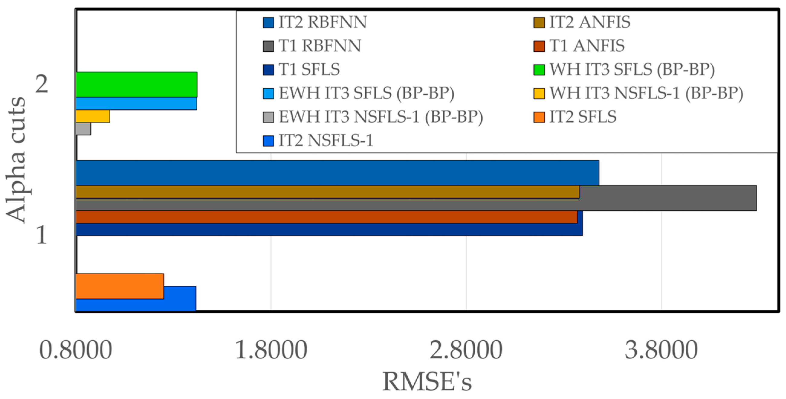
| Fuzzy System∖-Cuts | 1 | 2 |
|---|---|---|
| T1 SFLS | 3.39596 | |
| T1 ANFIS | 3.36958 | |
| T1 RBFNN | 4.28737 | |
| IT2 SFLS | 1.4249 | |
| IT2 NSFLS-1 | 1.2542 | |
| IT2 ANFIS | 3.37824 | |
| IT2 RBFNN | 3.47980 | |
| IT2 NSFLS-1 | 1.2542 | |
| WH IT3 SFLS (BP–BP) | 1.4212 | |
| EWH IT3 SFLS (BP–BP) | 1.4192 | |
| WH IT3 NSFLS-1 (BP–BP) | 0.9729 | |
| EWH IT3 NSFLS-1 (BP–BP) | 0.8761 |
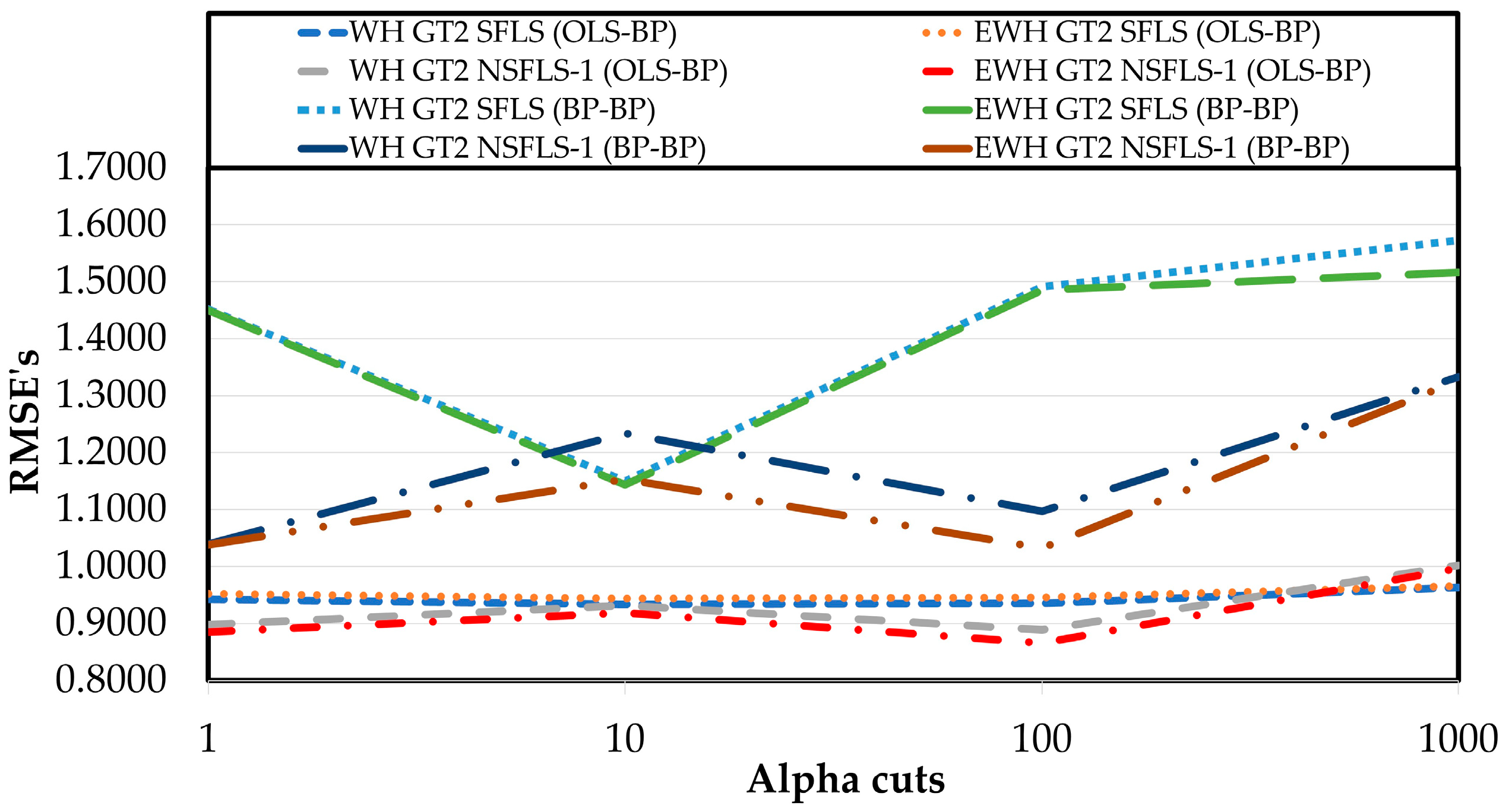
| Fuzzy System∖-Cuts | 1 | 10 | 100 | 1000 |
|---|---|---|---|---|
| IT2 SFLS | 1.4249 | |||
| IT2 NSFLS-1 | 1.2542 | |||
| WH GT2 SFLS (BP–BP) | 1.4515 | 1.1501 | 1.4912 | 1.5727 |
| EWH GT2 SFLS (BP–BP) | 1.4497 | 1.1433 | 1.4852 | 1.5166 |
| WH GT2 NSFLS-1 (BP–BP) | 1.0397 | 1.2338 | 1.097 | 1.3325 |
| EWH GT2 NSFLS-1 (BP–BP) | 1.0383 | 1.1534 | 1.0321 | 1.326 |
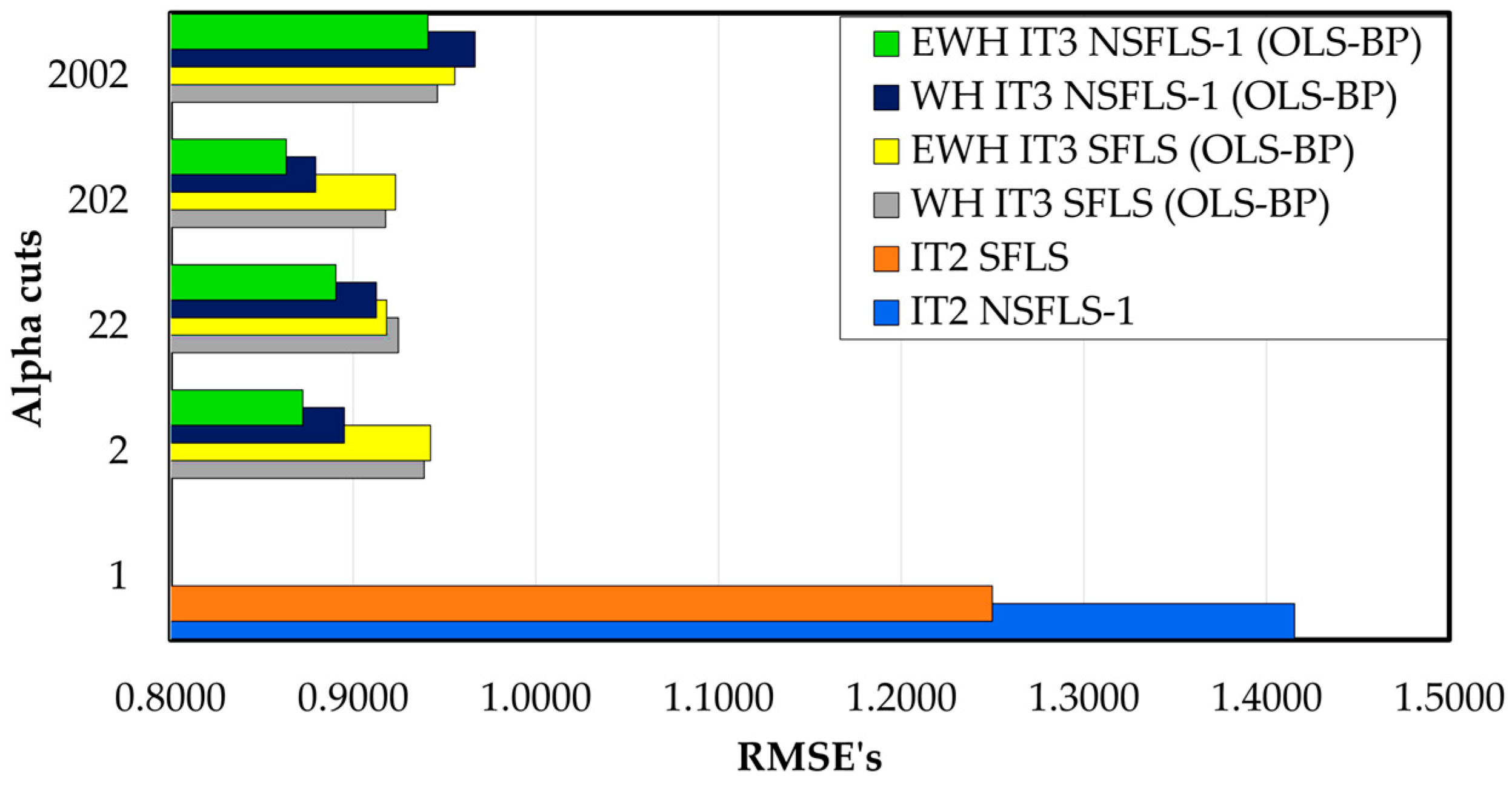
| Fuzzy System∖-Cuts | 1 | 2 | 22 | 202 | 2002 |
|---|---|---|---|---|---|
| IT2 SFLS | 1.4249 | ||||
| IT2 NSFLS-1 | 1.2542 | ||||
| WH IT3 SFLS (BP–BP) | 1.4212 | 1.0573 | 1.4063 | 1.4568 | |
| EWH IT3 SFLS (BP–BP) | 1.4192 | 1.0528 | 1.4016 | 1.4239 | |
| WH IT3 NSFLS-1 (BP–BP) | 0.9729 | 1.1107 | 1.0547 | 1.2197 | |
| EWH IT3 NSFLS-1 (BP–BP) | 0.8761 | 1.0125 | 1.0275 | 1.168 |
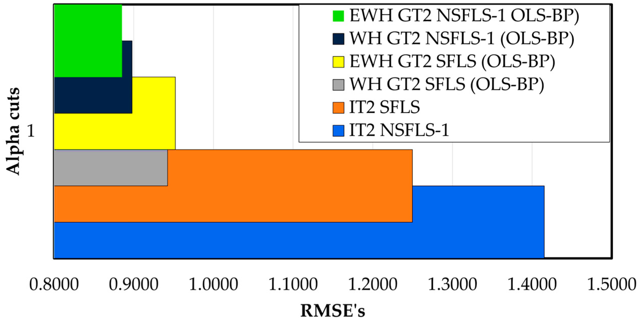
| Fuzzy System∖-Cuts | 1 |
|---|---|
| IT2 SFLS | 1.4249 |
| IT2 NSFLS-1 | 1.2542 |
| WH GT2 SFLS (OLS–BP) | 0.9389 |
| EWH GT2 SFLS (OLS–BP) | 0.9424 |
| WH GT2 NSFLS-1 (OLS–BP) | 0.8952 |
| EWH GT2 NSFLS-1 (OLS–BP) | 0.8724 |
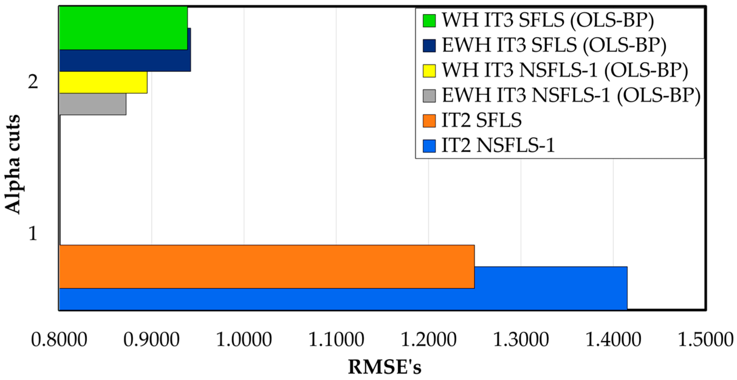
| Fuzzy Systems∖-Cuts | 1 | 2 |
|---|---|---|
| IT2 SFLS | 1.4249 | |
| IT2 NSFLS-1 | 1.2542 | |
| WH IT3 SFLS (OLS–BP) | 0.9389 | |
| EWH IT3 SFLS (OLS–BP) | 0.9424 | |
| WH IT3 NSFLS-1 (OLS–BP) | 0.8952 | |
| EWH IT3 NSFLS-1 (OLS–BP) | 0.8724 |
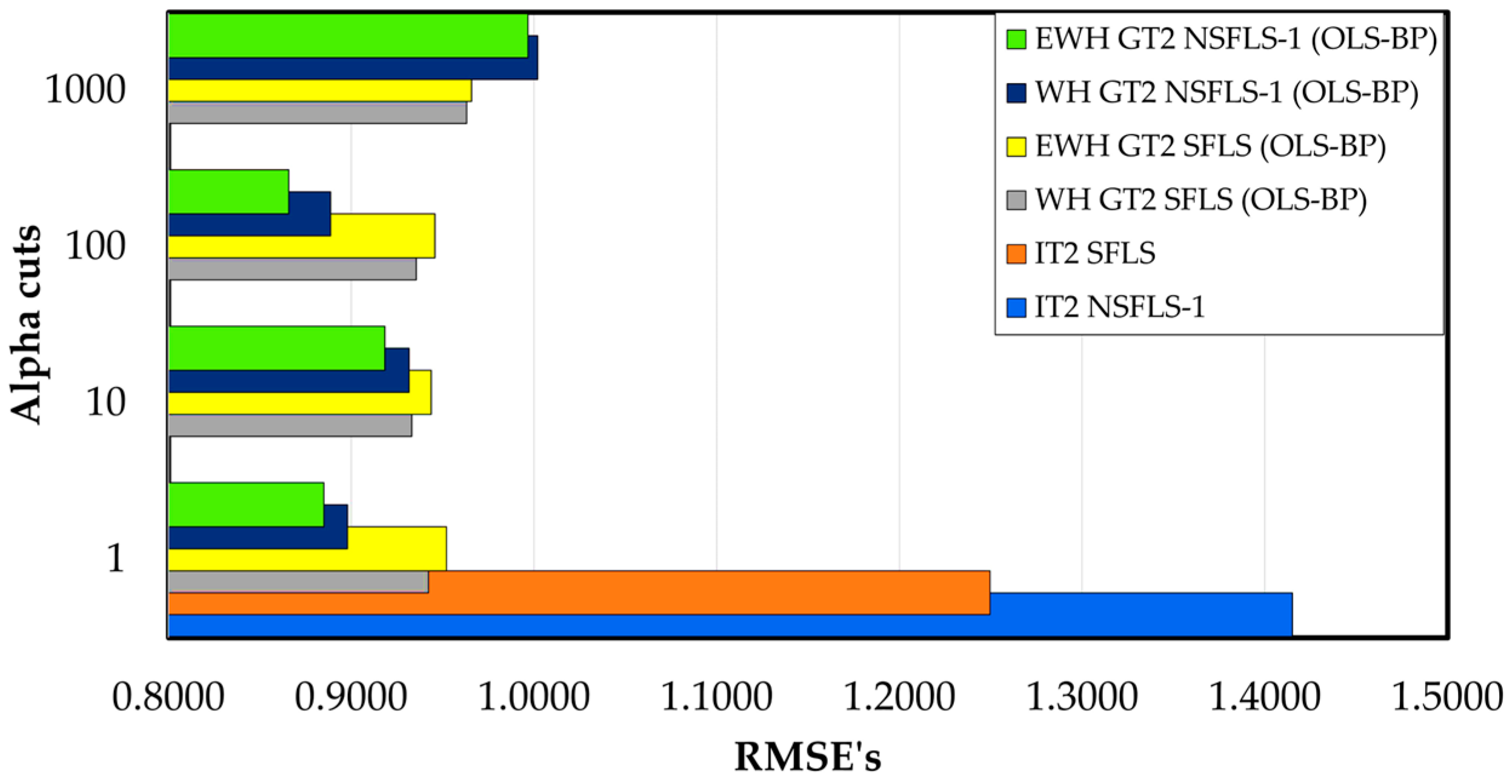
| Fuzzy System∖-Cuts | 1 | 10 | 100 | 1000 |
|---|---|---|---|---|
| IT2 SFLS | 1.4249 | |||
| IT2 NSFLS-1 | 1.2542 | |||
| WH GT2 SFLS (OLS–BP) | 0.9424 | 0.9332 | 0.9356 | 0.9631 |
| EWH GT2 SFLS (OLS–BP) | 0.9521 | 0.9438 | 0.9458 | 0.9658 |
| WH GT2 NSFLS-1 (OLS–BP) | 0.8979 | 0.9316 | 0.8888 | 1.002 |
| EWH GT2 NSFLS1 (OLS–BP) | 0.8851 | 0.9183 | 0.8659 | 0.9967 |
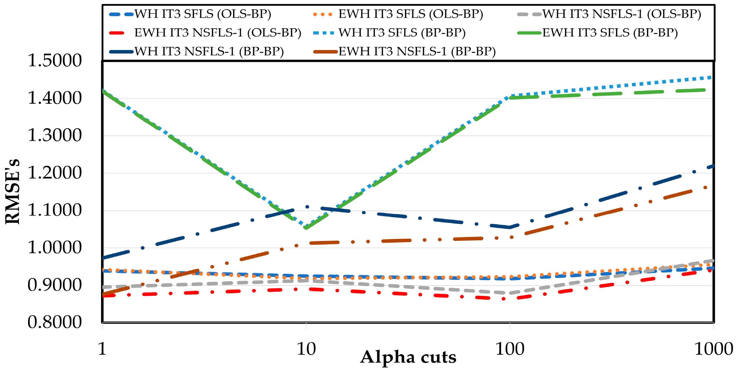
| Fuzzy System∖-Cuts | 1 | 2 | 10 | 100 | 1000 |
|---|---|---|---|---|---|
| IT2 SFLS | 1.4249 | ||||
| IT2 NSFLS-1 | 1.2542 | ||||
| WH IT3 SFLS (OLS–BP) | 0.9389 | 0.9247 | 0.9177 | 0.9461 | |
| EWH IT3 SFLS (OLS–BP) | 0.9424 | 0.9184 | 0.9231 | 0.9556 | |
| WH IT3 NSFLS-1 (OLS–BP) | 0.8952 | 0.9127 | 0.8795 | 0.9666 | |
| EWH IT3 NSFLS-1 (OLS–BP) | 0.8724 | 0.8905 | 0.8634 | 0.9408 |
Disclaimer/Publisher’s Note: The statements, opinions and data contained in all publications are solely those of the individual author(s) and contributor(s) and not of MDPI and/or the editor(s). MDPI and/or the editor(s) disclaim responsibility for any injury to people or property resulting from any ideas, methods, instructions or products referred to in the content. |
© 2023 by the authors. Licensee MDPI, Basel, Switzerland. This article is an open access article distributed under the terms and conditions of the Creative Commons Attribution (CC BY) license (https://creativecommons.org/licenses/by/4.0/).
Share and Cite
Méndez, G.M.; López-Juárez, I.; Alcorta García, M.A.; Martinez-Peon, D.C.; Montes-Dorantes, P.N. The Enhanced Wagner–Hagras OLS–BP Hybrid Algorithm for Training IT3 NSFLS-1 for Temperature Prediction in HSM Processes. Mathematics 2023, 11, 4933. https://doi.org/10.3390/math11244933
Méndez GM, López-Juárez I, Alcorta García MA, Martinez-Peon DC, Montes-Dorantes PN. The Enhanced Wagner–Hagras OLS–BP Hybrid Algorithm for Training IT3 NSFLS-1 for Temperature Prediction in HSM Processes. Mathematics. 2023; 11(24):4933. https://doi.org/10.3390/math11244933
Chicago/Turabian StyleMéndez, Gerardo Maximiliano, Ismael López-Juárez, María Aracelia Alcorta García, Dulce Citlalli Martinez-Peon, and Pascual Noradino Montes-Dorantes. 2023. "The Enhanced Wagner–Hagras OLS–BP Hybrid Algorithm for Training IT3 NSFLS-1 for Temperature Prediction in HSM Processes" Mathematics 11, no. 24: 4933. https://doi.org/10.3390/math11244933
APA StyleMéndez, G. M., López-Juárez, I., Alcorta García, M. A., Martinez-Peon, D. C., & Montes-Dorantes, P. N. (2023). The Enhanced Wagner–Hagras OLS–BP Hybrid Algorithm for Training IT3 NSFLS-1 for Temperature Prediction in HSM Processes. Mathematics, 11(24), 4933. https://doi.org/10.3390/math11244933