A New Incommensurate Fractional-Order COVID 19: Modelling and Dynamical Analysis

Abstract

Nowadays, a lot of research papers are concentrating on the diffusion dynamics of infectious diseases, especially the most recent one: COVID-19. The primary goal of this work is to explore the stability analysis of a new version of the $SEIR$ model formulated with incommensurate fractional-order derivatives. In particular, several existence and uniqueness results of the solution of the proposed model are derived by means of the Picard–Lindelöf method. Several stability analysis results related to the disease-free equilibrium of the model are reported in light of computing the so-called basic reproduction number, as well as in view of utilising a certain Lyapunov function. In conclusion, various numerical simulations are performed to confirm the theoretical findings.

1. Introduction

Coronavirus disease is an acute severe breathing disease resulting from a coronavirus 2 (SARS-CoV-2), which represents a novel component of the family Coronaviridae and the genus Beta coronavirus [1,2]. This virus is mainly transmitted from one human being to another through contact transmission and airborne droplets [3]. The clinical signs of the infected clients appear as severe, moderate, and mild symptoms such as pneumonia, diarrhoea, nausea, new loss of smell or taste, fatigue, difficulty breathing, dry cough, and fever [4,5]. Extremely harsh cases, presenting as organ dysfunctions, chronic medical illness, and death, have often been witnessed in people with immunodeficiencies and elderly patients [6]. The pandemic began spreading in China and then transmitted broadly to communities around the world [7,8].

In view of the fact that the number of confirmed cases of COVID-19 continues to grow, predictions of the number of infected individuals, as well as the COVID-19 pandemic’s ending, are indeed worthy of further examination. From this perspective, mathematical modelling of such a disease can play a key role in investigating its spread dynamics. In general, a mathematical model can provide a sufficient prediction to the outbreak’s coming conditions, enabling decision makers to implement excellent strategies for controlling the spread of diseases. In [9], the authors make a contribution to the mathematical theory of the spread of epidemics and the causes and triggers of the spread. Meanwhile, [10] presents an analytical study and simulation of the model of the spread of epidemics in complex networks. The paper [11] gives an explanation for periodic solutions in epidemiological models. In fact, there are many kinds of mathematical models that can be used to provide a good prediction for the infection spread of pandemics and biological invasions. Among them are what we named the compartment models. This kind of model has confirmed its top position in describing and understanding the complex spread of COVID-19 dynamics. In this paper, we establish a novel version of the SEIR model with incommensurate fractional-order derivatives; the fractional order is characterised by the effect of memory, which allows us to provide more accurate results than the usual derivatives [12]. It is a well-known fact that this model has four main compartments involving the susceptible cases S, exposed cases E, infectious cases I, and recovered cases R. The $SEIR$ model has confirmed its ability to describe the transmission of disease from one infected human to another one in a short period of time. Several investigators have examined the prediction dynamics of various $SEIR$ models, such as severe acute respiratory syndrome [13,14], Middle East respiratory syndrome [15,16], Ebola [17,18], and Dengue fever [19,20,21], to name a few.

Recently, many works have expressed interested in models describing the spread of the COVID-19 virus, in the discrete cases [22] and fractional-order discrete cases [23,24,25,26,27,28,29], and most of their interest was in studying the dynamics of these systems. Some models showed that they have chaotic behavior [30].

In this work, we intend to present a sufficient study that deals with the stability analysis of a new version of the $SEIR$ model formulated with incommensurate fractional-order derivatives. Actually, the initial version of the $SEIR$ model at hand was first proposed in [31] as follows:

$$\left\{\begin{array}{cc}\frac{dS}{dt}=\hfill & \mathsf{\Lambda }-r_1\frac{S\left(t\right)E\left(t\right)}{N\left(t\right)}-r_2\frac{S\left(t\right)I\left(t\right)}{N\left(t\right)}-\mu S\left(t\right)+\tau R\left(t\right),\hfill \\ \frac{dE}{dt}=\hfill & r_1\frac{S\left(t\right)E\left(t\right)}{N\left(t\right)}+r_2\frac{S\left(t\right)I\left(t\right)}{N\left(t\right)}-(\mu +\rho )E\left(t\right),\hfill \\ \frac{dI}{dt}=\hfill & \rho E\left(t\right)-(\gamma +d+\mu )I\left(t\right),\hfill \\ \frac{dR}{dt}=\hfill & \gamma I\left(t\right)-(\mu +\tau )R\left(t\right),\hfill \end{array}\right.$$

(1)

where the model’s description with its parameters can be outlined in

Table 1. Description of the $SEIR$ model reported in [31].

Variable/Parameter	Description
$S\left(t\right)$	Susceptible class
$E\left(t\right)$	Exposed class
$I\left(t\right)$	Infected class
$R\left(t\right)$	Recovered class
$\mathsf{\Lambda }$	Recruitment rate into susceptible population
$r_1,r_2$	Incidence rates
$\mu$	Natural mortality rate
$\tau$	Relapse rate
$\rho$	Progression rate from exposed to infectious class
$\gamma$	Treatment rate for infectious individuals
d	COVID-19 death rate

, reported below.

The total population N can be gained by adding up all classes announced in the model (1), i.e.,

$$N=S+E+I+R.$$

(2)

Over the last few decades, fractional calculus has demonstrated immense effectiveness in providing more sensible outcomes than that of traditional calculus. This is, however, connected to its flexibility in offering accurate approximations to several solutions of a lot of real phenomena and several applied science problems which are better than those that came before. From this point of view, we will pay attention to the model that could be formulated by fractionalising model (1) in the sense of the Caputo incommensurate fractional-order derivative operator. This model, in brief, would take the following form:

$$\left\{\begin{array}{cc}{}_0^C{D}_t^{{\alpha }_1}S\left(t\right)=\hfill & \mathsf{\Lambda }-r_1\frac{S\left(t\right)E\left(t\right)}{N\left(t\right)}-r_2\frac{S\left(t\right)I\left(t\right)}{N\left(t\right)}-\mu S\left(t\right)+\tau R\left(t\right),\hfill \\ {}_0^C{D}_t^{{\alpha }_2}E\left(t\right)=\hfill & r_1\frac{S\left(t\right)E\left(t\right)}{N\left(t\right)}+r_2\frac{S\left(t\right)I\left(t\right)}{N\left(t\right)}-(\mu +\rho )E\left(t\right),\hfill \\ {}_0^C{D}_t^{{\alpha }_3}I\left(t\right)=\hfill & \rho E\left(t\right)-(\gamma +d+\mu )I\left(t\right),\hfill \\ {}_0^C{D}_t^{{\alpha }_4}R\left(t\right)=\hfill & \gamma I\left(t\right)-(\mu +\tau )R\left(t\right),\hfill \end{array}\right.$$

(3)

subject to the following initial conditions:

$$S\left(0\right),E\left(0\right),I\left(0\right),R\left(0\right)\ge 0,$$

(4)

where $0<{\alpha }_1,{\alpha }_2,{\alpha }_3,{\alpha }_4<1$ and ${}_{t_0}^C{D}_t^{\alpha }$ is the Caputo fractional-order derivative operator, which will be presented in the next section.

2. Preliminaries

To proceed to the main objectives, some needed facts and definitions from fractional calculus are collected in the following paragraphs.

Definition 1

([32]). The Riemann–Liouville fractional-order integral operator of an arbitrary integrable function f can be expressed as:

$$I_t^{\alpha }f\left(t\right)=\frac{1}{\mathsf{\Gamma }\left(\alpha \right)}{\int }_{t_0}^t{(t-\tau )}^{\alpha -1}f\left(\tau \right)d\tau ,$$

(5)

where $t\ge t_0$, $0<\alpha <1$, and $\mathsf{\Gamma }(·)$ is the gamma function.

Definition 2

([32]). The Caputo fractional-order derivative operator of the function f can be expressed as:

$${}_{t_0}^C{D}_t^{\alpha }f\left(t\right)=\frac{1}{\mathsf{\Gamma }(1-\alpha )}{\int }_{t_0}^t{(t-\tau )}^{-\alpha }\frac{d}{d\tau }f\left(\tau \right)d\tau ,$$

(6)

where $0<\alpha <1$

For simplicity, we intend to choose the notion ${}^C{D}_t^{\alpha }$ instead of ${}_{t_0}^C{D}_t^{\alpha }$ throughout the remainder of this paper.

Lemma 1

([33]). (Generalised mean value theorem). Suppose that $f\left(t\right)\in C\left(\right[a,b\left]\right)$ and ${}^C{D}_t^{\alpha }f\left(t\right)\in C\left(\right]a,b\left]\right)$, such that $0<\alpha \le 1$, then:

$$f\left(t\right)=f\left(a\right)+\frac{1}{\mathsf{\Gamma }\left(\alpha \right)}{}^C{D}_t^{\alpha }f\left(\xi \right){(t-a)}^{\alpha },$$

(7)

with $a\le \xi \le t$, for all $t\in (a,b]$.

3. Existence and Uniqueness Results

In this part, some theoretical results associated with the existence and uniqueness of the solution of the proposed system (3) are derived with the help of the fixed-point theory and Picard–Lindelöf method. To go forward to this goal, we may rewrite system (3) in the following classical form:

$$\left\{\begin{array}{cc}{}_0^C{D}_t^{{\alpha }_1}S\left(t\right)=\hfill & F_1(t,S)\hfill \\ {}_0^C{D}_t^{{\alpha }_2}E\left(t\right)=\hfill & F_2(t,E)\hfill \\ {}_0^C{D}_t^{{\alpha }_3}I\left(t\right)=\hfill & F_3(t,I)\hfill \\ {}_0^C{D}_t^{{\alpha }_4}R\left(t\right)=\hfill & F_5(t,R)\hfill \end{array}\right.$$

(8)

where the functions $F_i$, $1\le i\le 4$, are defined as follows:

$$\begin{array}{cc}{F}_1(t,S)=\hfill & \mathsf{\Lambda }-r_1\frac{S\left(t\right)E\left(t\right)}{N\left(t\right)}-r_2\frac{S\left(t\right)I\left(t\right)}{N\left(t\right)}-\mu S\left(t\right)+\tau R\left(t\right),\hfill \\ F_2(t,E)=\hfill & r_1\frac{S\left(t\right)E\left(t\right)}{N\left(t\right)}+r_2\frac{S\left(t\right)I\left(t\right)}{N\left(t\right)}-(\mu +\rho )E\left(t\right),\hfill \\ F_3(t,I)=\hfill & \rho E\left(t\right)-(\gamma +d+\mu )I\left(t\right),\hfill \\ F_5(t,R)=\hfill & \gamma I\left(t\right)-(\mu +\tau )R\left(t\right).\hfill \end{array}$$

(9)

In consequence, we proceed in the following manner. We first use the initial conditions given in (4), and then we apply the fractional-order integral operator given in (5) on system (3). This would transform its equations to be as follows:

$$\left\{\begin{array}{cc}S\left(t\right)-S\left(0\right)=\hfill & I_t^{{\alpha }_1}\left(\mathsf{\Lambda }-r_1\frac{S\left(t\right)E\left(t\right)}{N\left(t\right)}-r_2\frac{S\left(t\right)I\left(t\right)}{N\left(t\right)}-\mu S\left(t\right)+\tau R\left(t\right)\right),\hfill \\ E\left(t\right)-E\left(0\right)=\hfill & I_t^{{\alpha }_2}\left(r_1\frac{S\left(t\right)E\left(t\right)}{N\left(t\right)}+r_2\frac{S\left(t\right)I\left(t\right)}{N\left(t\right)}-(\mu +\rho )E\left(t\right)\right),\hfill \\ I\left(t\right)-I\left(0\right)=\hfill & I_t^{{\alpha }_3}\left(\rho E\left(t\right)-(\gamma +d+\mu )I\left(t\right)\right),\hfill \\ R\left(t\right)-R\left(0\right)=\hfill & I_t^{{\alpha }_4}\left(\gamma I\left(t\right)-(\mu +\tau )R(t\right)).\hfill \end{array}\right.$$

(10)

With the help of (9), we can obtain the state variables in terms of $F_i$, $i=1,2,3,4$, as follows:

$$\left\{\begin{array}{cc}S\left(t\right)=\hfill & S\left(0\right)+\frac{1}{\mathsf{\Gamma }\left({\alpha }_1\right)}{\int }_0^t{(t-s)}^{{\alpha }_1-1}{F}_1(s,S\left(s\right))ds,\hfill \\ E\left(t\right)=\hfill & E\left(0\right)+\frac{1}{\mathsf{\Gamma }\left({\alpha }_2\right)}{\int }_0^t{(t-s)}^{{\alpha }_2-1}{F}_2(s,E\left(s\right))ds,\hfill \\ I\left(t\right)=\hfill & I\left(0\right)+\frac{1}{\mathsf{\Gamma }\left({\alpha }_3\right)}{\int }_0^t{(t-s)}^{{\alpha }_3-1}{F}_3(s,I\left(s\right))ds,\hfill \\ R\left(t\right)=\hfill & R\left(0\right)+\frac{1}{\mathsf{\Gamma }\left({\alpha }_4\right)}{\int }_0^t{(t-s)}^{{\alpha }_4-1}{F}_4(s,R\left(s\right))ds.\hfill \end{array}\right.$$

(11)

Accordingly, the Picard iterations can be then implemented to (11) to gain the following equations:

$$\left\{\begin{array}{cc}{S}_{n+1}\left(t\right)=\hfill & S\left(0\right)+\frac{1}{\mathsf{\Gamma }\left({\alpha }_1\right)}{\int }_0^t{(t-s)}^{{\alpha }_1-1}{F}_1(s,S_n\left(s\right))ds,\hfill \\ E_{n+1}\left(t\right)=\hfill & E\left(0\right)+\frac{1}{\mathsf{\Gamma }\left({\alpha }_2\right)}{\int }_0^t{(t-s)}^{{\alpha }_2-1}{F}_2(s,E_n\left(s\right))ds,\hfill \\ I_{n+1}\left(t\right)=\hfill & I\left(0\right)+\frac{1}{\mathsf{\Gamma }\left({\alpha }_3\right)}{\int }_0^t{(t-s)}^{{\alpha }_3-1}{F}_3(s,I_n\left(s\right))ds,\hfill \\ R_{n+1}\left(t\right)=\hfill & R\left(0\right)+\frac{1}{\mathsf{\Gamma }\left({\alpha }_4\right)}{\int }_0^t{(t-s)}^{{\alpha }_4-1}{F}_4(s,R_n\left(s\right))ds.\hfill \end{array}\right.$$

(12)

In order to discuss the first result, we let $X\left(t\right)={\left(S\left(t\right),E\left(t\right),I\left(t\right),R\left(t\right)\right)}^T$, $F(t,X\left(t\right))={\left(F_1(t,S\left(t\right)),F_2(t,E\left(t\right)),F_3(t,I\left(t\right)),F_4(t,R\left(t\right))\right)}^T$ and ${\mathbb{R}}_{+}^4=\left\{X\in {\mathbb{R}}^4:X\ge 0\right\}$.

Lemma 2.

The solution of system (3) (if it exists) with non-negative initial data will remain non-negative.

Proof. 

For the purpose of proving this result, we should first observe that the following assertions hold:

$$\begin{array}{cc}{\left.{}_0^C{D}_t^{{\alpha }_1}S\left(t\right)\right|}_{S=0}=\hfill & \mathsf{\Lambda }+\tau R\left(t\right)\ge 0,\hfill \\ {\left.{}_0^C{D}_t^{{\alpha }_2}E\left(t\right)\right|}_{E=0}=\hfill & r_2\frac{S\left(t\right)I\left(t\right)}{N\left(t\right)}\ge 0,\hfill \\ {\left.{}_0^C{D}_t^{{\alpha }_3}I\left(t\right)\right|}_{I=0}=\hfill & \rho E\left(t\right)\ge 0,\hfill \\ {\left.{}_0^C{D}_t^{{\alpha }_4}R\left(t\right)\right|}_{R=0}=\hfill & \gamma I\left(t\right)\ge 0,\hfill \end{array}$$

(13)

for all $t\in [0,T]$. Consequently, according to Lemma 1, we can conclude that the solution $X\left(t\right)={(S\left(t\right),E\left(t\right),I\left(t\right),R\left(t\right))}^T$ of system (3) belongs to ${\mathbb{R}}_{+}^4$, and this completes the proof. □

In the following content, we aim to state and prove one of the significant results of this work. Actually, this result will pave the way to derive the result that discusses the existence and uniqueness of the solution of system (3), which will be provided later on.

Lemma 3.

The function $F(t,X(t\left)\right)$ defined in (9) satisfies the Lipschitz condition, i.e.,

$$∥F(t,X\left(t\right))-F(t,X^{*}\left(t\right))∥\le \beta ∥\left(X\left(t\right)-X^{*}\left(t\right)\right)∥,$$

(14)

where

$$\beta =max\left\{\left|r_1+r_2+\mu \right|,\left|r_1+\mu +\rho \right|,\left|(\gamma +d+\mu )\right|,\left|(\mu +\tau )\right|\right\}.$$

(15)

Proof. 

Summarising that $S\left(t\right)$ and $S^{*}\left(t\right)$ are couple functions yields the following equality:

$$∥F_1(t,S\left(t\right))-F_1(t,S^{*}\left(t\right))∥=∥\left(r_1\frac{E\left(t\right)}{N\left(t\right)}+r_2\frac{I\left(t\right)}{N\left(t\right)}+\mu \right)\left(S\left(t\right)-S^{*}\left(t\right)\right)∥.$$

(16)

Considering

$${\beta }_1=\left|r_1+r_2+\mu \right|$$

(17)

leads one to deduce the following inequality:

$$∥F_1(t,S\left(t\right))-F_1(t,S^{*}\left(t\right))∥\le {\beta }_1∥\left(S\left(t\right)-S^{*}\left(t\right)\right)∥.$$

(18)

Continuing in the same way, one gets:

$$\begin{array}{cc}∥F_2(t,E\left(t\right))-F_1(t,E^{*}\left(t\right))∥\le \hfill & {\beta }_2∥\left(E\left(t\right)-E^{*}\left(t\right)\right)∥,\hfill \\ ∥F_3(t,I\left(t\right))-F_1(t,I^{*}\left(t\right))∥\le \hfill & {\beta }_3∥\left(I\left(t\right)-I^{*}\left(t\right)\right)∥,\hfill \\ ∥F_5(t,R\left(t\right))-F_1(t,R^{*}\left(t\right))∥\le \hfill & {\beta }_4∥\left(R\left(t\right)-R^{*}\left(t\right)\right)∥,\hfill \end{array}$$

(19)

where

$$\begin{array}{cc}{\beta }_2=\hfill & \left|r_1+\mu +\rho \right|,\hfill \\ {\beta }_3=\hfill & \left|\gamma +d+\mu \right|,\hfill \\ {\beta }_4=\hfill & \left|\mu +\tau \right|.\hfill \end{array}$$

(20)

From (18–19), we find that all four kernels, $F_1,F_2,F_3$, and $F_4$, satisfy the Lipschitz condition. In addition, we also notice that if ${\beta }_i<1$, then the kernels $F_i$s are contradictory for $i=1,2,3,4$. □

Theorem 1.

Consider Lemma 3. If

$$\beta \underset{1\le i\le 4}{max}\frac{T^{{\alpha }_i}}{\mathsf{\Gamma }({\alpha }_i+1)}<1,$$

(21)

then there exists a unique positive solution of system (3).

Proof. 

In fact, the solution of system (3) can be written as:

$$X\left(t\right)=P\left(X\right(t\left)\right),$$

(22)

where $P:C([0,T],{\mathbb{R}}^4)\to C([0,T],{\mathbb{R}}^4)$ is the Picard operator, which can be defined by:

$$P\left(X\left(t\right)\right)=X\left(0\right)+{\int }_0^{t}diag\left(\frac{{(t-s)}^{{\alpha }_1-1}}{\mathsf{\Gamma }\left({\alpha }_1\right)},\frac{{(t-s)}^{{\alpha }_2-1}}{\mathsf{\Gamma }\left({\alpha }_2\right)},\frac{{(t-s)}^{{\alpha }_3-1}}{\mathsf{\Gamma }\left({\alpha }_3\right)},\frac{{(t-s)}^{{\alpha }_4-1}}{\mathsf{\Gamma }\left({\alpha }_4\right)}\right)F(s,X\left(s\right))ds.$$

(23)

At the same time, we have the following consecutive inequalities:

$$\begin{array}{ccc}∥P(X\left(t\right)-P\left(X^{*}\left(t\right)\right)∥\hfill & =\hfill & \begin{array}{c}∥{\int }_0^{t}diag\left(\frac{{(t-s)}^{{\alpha }_1-1}}{\mathsf{\Gamma }\left({\alpha }_1\right)},\frac{{(t-s)}^{{\alpha }_2-1}}{\mathsf{\Gamma }\left({\alpha }_2\right)},\frac{{(t-s)}^{{\alpha }_3-1}}{\mathsf{\Gamma }\left({\alpha }_3\right)},\frac{{(t-s)}^{{\alpha }_4-1}}{\mathsf{\Gamma }\left({\alpha }_4\right)}\right)\hfill \\ \times \left(F(s,X\left(s\right))-F(s,X^{*}\left(s\right))\right)ds∥\hfill \end{array},\hfill \\ \hfill & \le \hfill & \begin{array}{c}∥{\int }_0^{t}diag\left(\frac{{(t-s)}^{{\alpha }_1-1}}{\mathsf{\Gamma }\left({\alpha }_1\right)},\frac{{(t-s)}^{{\alpha }_2-1}}{\mathsf{\Gamma }\left({\alpha }_2\right)},\frac{{(t-s)}^{{\alpha }_3-1}}{\mathsf{\Gamma }\left({\alpha }_3\right)},\frac{{(t-s)}^{{\alpha }_4-1}}{\mathsf{\Gamma }\left({\alpha }_4\right)}\right)ds∥\hfill \\ \times {\displaystyle \underset{s\in [0,T]}{sup}}∥F(s,X\left(s\right))-F(s,X^{*}\left(s\right))∥\hfill \end{array}\hfill \\ \hfill & \le \hfill & {\displaystyle \underset{1\le i\le 4}{max}}{\int }_0^t\frac{{(t-s)}^{{\alpha }_i-1}}{\mathsf{\Gamma }\left({\alpha }_i\right)}ds{\displaystyle \underset{s\in [0,T]}{sup}}∥F(s,X\left(s\right))-F(s,X^{*}\left(s\right))∥,\hfill \\ \hfill & \le \hfill & \beta {\displaystyle \underset{1\le i\le 4}{max}}\frac{T^{{\alpha }_i}}{\mathsf{\Gamma }({\alpha }_i+1)}{\displaystyle \underset{s\in [0,T]}{sup}}∥X\left(t\right)-X^{*}\left(t\right)∥.\hfill \end{array}$$

(24)

Since $\beta {\displaystyle \underset{1\le i\le 4}{max}}\frac{T^{{\alpha }_i}}{\mathsf{\Gamma }({\alpha }_i+1)}<1$, for $t\le T$, then the operator P is a contraction. Hence, system (3) has a unique solution, which finishes the proof of this result. □

4. Stability Analysis of the Model

This part is devoted to deriving various stability analysis results related to the incommensurate fractional-order COVID-9 model (3). Such results are associated with determining the disease-free equilibrium (DFE) point and calculating the basic reproduction number $R_0$.

4.1. Disease-Free Equilibrium (DFE)

It may be stated that identifying the equilibrium points of the $SEIR$ models is deemed one of the key points necessary to investigate their stability analysis. As a matter of fact, there exist two primary types of such equilibria that may be categorised in accordance with the non-existence of the infection: the Endemic Equilibrium (EE) point and the Disease-Free Equilibrium (DFE) point. In particular, to find the DFE point for system (3), we set its right-hand side to be equal to 0, together with letting $I=0$. In other words, we let ${}_0^C{D}_t^{{\alpha }_1}S\left(t\right)=0$, ${}_0^C{D}_t^{{\alpha }_2}E\left(t\right)=0$, ${}_0^C{D}_t^{{\alpha }_3}I\left(t\right)=0$, ${}_0^C{D}_t^{{\alpha }_4}R\left(t\right)=0$. Thus, system (3) is:

$$\left\{\begin{array}{c}\mathsf{\Lambda }-r_1\frac{SE}{N}-r_2\frac{SI}{N}-\mu S+\tau R=0,\\ r_1\frac{SE}{N}+r_2\frac{SI}{N}-(\mu +\rho )E=0,\\ \rho E-(\gamma +d+\mu )I=0,\\ \gamma I-(\mu +\tau )R=0.\end{array}\right.$$

(25)

This immediately gives rise to the equilibrium point:

$$E_F=(S_0,0,0,0)=(\frac{\mathsf{\Lambda }}{\mu },0,0,0).$$

(26)

4.2. Basic Reproduction Number $R_0$

The basic reproduction number $R_0$ signifies the average amount of the secondary cases produced from the preliminary infective individuals within a community without resistance to the pandemic [22]. This vital measure has progressively represented a fundamental amount utilised for identifying the interventions force required to dominate pandemics. In epidemiological models, it is widely known that if $R_0>1$, then the disease will progressively broadcast in the susceptible community. In contrast, if $R_0<1$, then the susceptible community will never suffer from epidemics. The scheme of finding $R_0$ needs to determine the spectral radius $\sigma$ of the next-generation matrix. In other words, $R_0=\sigma \left(G\right)$, where G is the next-generation matrix; see [22] to get a full overview of the calculation of such measure. Herein, we briefly intend to describe how $R_0$ can be calculated. To this end, we consider the following two equations that are taken out from the system (3):

$$\left\{\begin{array}{cc}{}_0^C{D}_t^{{\alpha }_2}E\left(t\right)=\hfill & r_1\frac{S\left(t\right)E\left(t\right)}{N\left(t\right)}+r_2\frac{S\left(t\right)I\left(t\right)}{N\left(t\right)}-(\mu +\rho )E\left(t\right),\hfill \\ {}_0^C{D}_t^{{\alpha }_3}I\left(t\right)=\hfill & \rho E\left(t\right)-(\gamma +d+\mu )I\left(t\right),\hfill \end{array}\right.$$

(27)

In accordance with the above equations, we can determine the matrix $J^{*}$ that can be established based on the leaving fluxes from the infected compartment and the new fluxes of such a compartment. That is,

$$J^{*}=\left(\begin{array}{cc}{r}_1-(\mu +\rho )& r_2\\ \rho & -(\gamma +d+\mu )\end{array}\right).$$

(28)

Now, we can decompose the matrix J in terms of another two matrices, F and V, such that $J=F-V$. This yields:

$$F=\left(\begin{array}{cc}{r}_1& r_2\\ 0& 0\end{array}\right),$$

(29)

and

$$V=\left(\begin{array}{cc}(\mu +\rho )& 0\\ -\rho & (\gamma +d+\mu )\end{array}\right).$$

(30)

Consequently, we can generate the next-generation matrix $G=F{V}^{-1}$ to be in the following form:

$$G=F{V}^{-1}=\left(\begin{array}{cc}\frac{r_1}{\mu +\rho }+\rho \frac{r_2}{\left(\mu +\rho \right)\left(d+\gamma +\mu \right)}& \frac{r_2}{d+\gamma +\mu }\\ 0& 0\end{array}\right).$$

(31)

Therefore, the basic reproduction number $R_0$ will then be given by:

$$R_0=\sigma \left(G\right)=\frac{d{r}_1+\gamma r_1+\mu r_1+\rho r_2}{\left(\mu +\rho \right)\left(d+\gamma +\mu \right)}.$$

(32)

4.3. Stability Analysis

In this section, we aim to further study the stability analysis of system (3) around the DFE. In particular, we will provide some theoretical results associated with the local and global stability analysis of the system at hand around the DFE with the aid of $R_0$ computed in the previous subsection.

4.3.1. Local Stability of DFE

In this part, we will derive a significant result related to the local stability analysis of system (3) around the DFE. This shall be accomplished by bearing in mind the next important theorem.

Theorem 2

([34]). Assume that $0<{\alpha }_i<1$, for $i=1,2,\cdots ,n$. Let M be the lowest common multiple between $u_i$ and $v_i$ in which ${\alpha }_i=\frac{v_i}{u_i}$, where $u_i,v_i\in \mathbb{N}$, such that $(u_i,v_i)=1$, $\forall i=1,2,\cdots ,n$. If all the roots λ of

$$det\left(diag\left({\lambda }^{v_1},{\lambda }^{v_2},\cdots ,{\lambda }^{v_n}\right)-J\right)=0,$$

(33)

satisfies $|arg\lambda |>\frac{\pi }{2M}$, where J is the Jacobian matrix of F at the equilibrium. Then, the equilibrium of system (3) is locally asymptotically stable.

Theorem 3.

Suppose ${\alpha }_2={\alpha }_3=\alpha$. Then, the DFE ($E_F$) of system (3) is locally asymptotically stable if $R_0<1$.

Proof. 

The Jacobian matrix of F at $E_F$ is:

$$J\left(E_F\right)=\left(\begin{array}{cccc}-\mu & -r_1& -r_2& \tau \\ 0& r_1-(\mu +\rho )& r_2& 0\\ 0& \rho & -(\gamma +d+\mu )& 0\\ 0& 0& \gamma & -(\mu +\tau )\end{array}\right).$$

(34)

Consequently, we can obtain:

$$det\left(diag\left({\lambda }^{M{\alpha }_1},{\lambda }^{M{\alpha }_2},{\lambda }^{M{\alpha }_3},{\lambda }^{M{\alpha }_4}\right)-J\left(E_F\right)\right)=0$$

(35)

⇔

$$\left(\mu +{\lambda }^{M{\alpha }_1}\right)\left(\tau +\mu +{\lambda }^{M{\alpha }_4}\right)\left({\lambda }^{M{\alpha }_2+M{\alpha }_3}+B{\lambda }^{M{\alpha }_2}+C{\lambda }^{M{\alpha }_3}+D\right),$$

(36)

where $B=(\gamma +\mu +d)$, $C=\left(\mu +\rho \right)(1+\frac{\rho r_2}{\left(\mu +\rho \right)\left(d+\gamma +\mu \right)}-R_0)$, and $D=\left(\mu +\rho \right)\left(d+\gamma +\mu \right)$$\left(1-R_0\right)$. This immediately yields:

$$\begin{array}{c}\left(\mu +{\lambda }^{M{\alpha }_1}\right)=0\Rightarrow arg{\lambda }_{1,k}=\frac{\pi }{M{\alpha }_1}+2\frac{k\pi }{M{\alpha }_1}\\ \Rightarrow \left|arg{\lambda }_{1,k}\right|>\frac{\pi }{2M},k=0,1,\cdots ,M{\alpha }_1-1,\end{array}$$

(37)

and

$$\begin{array}{c}\left(\tau +\mu +{\lambda }^{M{\alpha }_4}\right)=0\Rightarrow arg{\lambda }_{2,k}=\frac{\pi }{M{\alpha }_4}+2\frac{k\pi }{M{\alpha }_4}\\ \Rightarrow \left|arg{\lambda }_{2,k}\right|>\frac{\pi }{2M},k=0,1,\cdots ,M{\alpha }_4-1.\end{array}$$

(38)

Suppose ${\alpha }_2={\alpha }_3=\alpha$; then, we obtain:

$$\left({\lambda }^{M{\alpha }_2+M{\alpha }_3}+B{\lambda }^{M{\alpha }_2}+C{\lambda }^{M{\alpha }_3}+D\right)=\left({\lambda }^{2M\alpha }+(B+C){\lambda }^{M\alpha }+D\right).$$

(39)

If $R_0<1$, then $(B+C)>0$ and $D>0$. This leads us to deduce:

$${(B+C)}^2-4D>0.$$

Thus, the roots $\left({\lambda }_3^{M\alpha },{\lambda }_4^{M\alpha }\right)$ of

$$\left({\lambda }^{2M\alpha }+(B+C){\lambda }^{M\alpha }+D\right)=0$$

(40)

are negative. This gives:

$$\begin{array}{c}arg{\lambda }_{4,k}=arg{\lambda }_{3,k}=\frac{\pi }{M\alpha }+2\frac{k\pi }{M\alpha }\\ \Rightarrow \left|arg{\lambda }_{4,k}\right|=\left|arg{\lambda }_{3,k}\right|>\frac{\pi }{2M},k=0,1,\cdots ,M\alpha -1.\end{array}$$

(41)

Therefore, according to Theorem 2, the FDE point is locally asymptotically stable if $R_0<1$. □

4.3.2. Global Stability of DFE

In a similar manner to the previous part, we will derive another important result related to the global stability analysis of system (3) around the DFE based on one of the major stability theorems reported below.

Theorem 4

([34]). Let $x=0$ be an equilibrium point for the fractional-order non-linear system (3). Let $V(t,x)$ be a Lyapunov function and ${\gamma }_i$$(i=1,2,3)$ be functions of class $\mathcal{K}$, such that:

$${\gamma }_1\left(∥x∥\right)\le V(t,x\left(t\right))\le {\gamma }_1\left(∥x∥\right)$$

(42)

and

$${}^C{D}_t^{\beta }V(t,x\left(t\right))\le -{\gamma }_3\left(∥x∥\right),$$

(43)

where $\beta \in (0,1)$. Then, the equilibrium point $x=0$ is asymptotically stable.

Theorem 5.

Suppose ${\alpha }_2={\alpha }_3=\alpha$. If $R_0<1$, then the pandemic will disappear.

Proof. 

Consider the Lyapunov function of the form:

$$L\left(t\right)={\theta }_{1}E\left(t\right)+{\theta }_{2}I\left(t\right),$$

(44)

where ${\theta }_1=\frac{1}{2}$, and ${\theta }_2=\frac{r_2}{(\gamma +d+\mu )}$. Differentiating L with respect to the time t yields the following consecutive inequalities:

$$\begin{array}{cc}{}_0^C{D}_t^{\alpha }L\left(t\right)\hfill & ={\theta }_1{}_0^C{D}_t^{\alpha }E\left(t\right)+{\theta }_2{}_0^C{D}_t^{\alpha }I\left(t\right),\hfill \\ \hfill & ={\theta }_1\left(r_1\frac{S\left(t\right)E\left(t\right)}{N\left(t\right)}+r_2\frac{S\left(t\right)I\left(t\right)}{N\left(t\right)}-(\mu +\rho )E\left(t\right)\right)+{\theta }_2\left(\rho E\left(t\right)-(\gamma +d+\mu )I\left(t\right)\right),\hfill \\ \hfill & \le \left({\theta }_1{r}_1+{\theta }_2\rho -(\mu +\rho )\right)E+\left({\theta }_1{r}_2-{\theta }_2(\gamma +d+\mu )\right)I,\hfill \\ \hfill & \le (\mu +\rho )\left(\frac{r_1}{2(\mu +\rho )}+\frac{r_2\rho }{(\mu +\rho )(\gamma +d+\mu )}-1\right)E+\left(-\frac{r_2}{2}\right)I,\hfill \\ \hfill & \le (\mu +\rho )\left(R_0-1\right)E+\left(-\frac{r_2}{2}\right)I.\hfill \end{array}$$

(45)

If $R_0<1,$ then $L\left(t\right)$ will be immediately negative. Therefore, according to Theorem 4, the pandemic will disappear. □

It should be noted that the conditions of the previous theorems do not relate to the fractional-order values. This, however, backs up the fact that these results are just generalisations of the results reported in the case of the integer-order values.

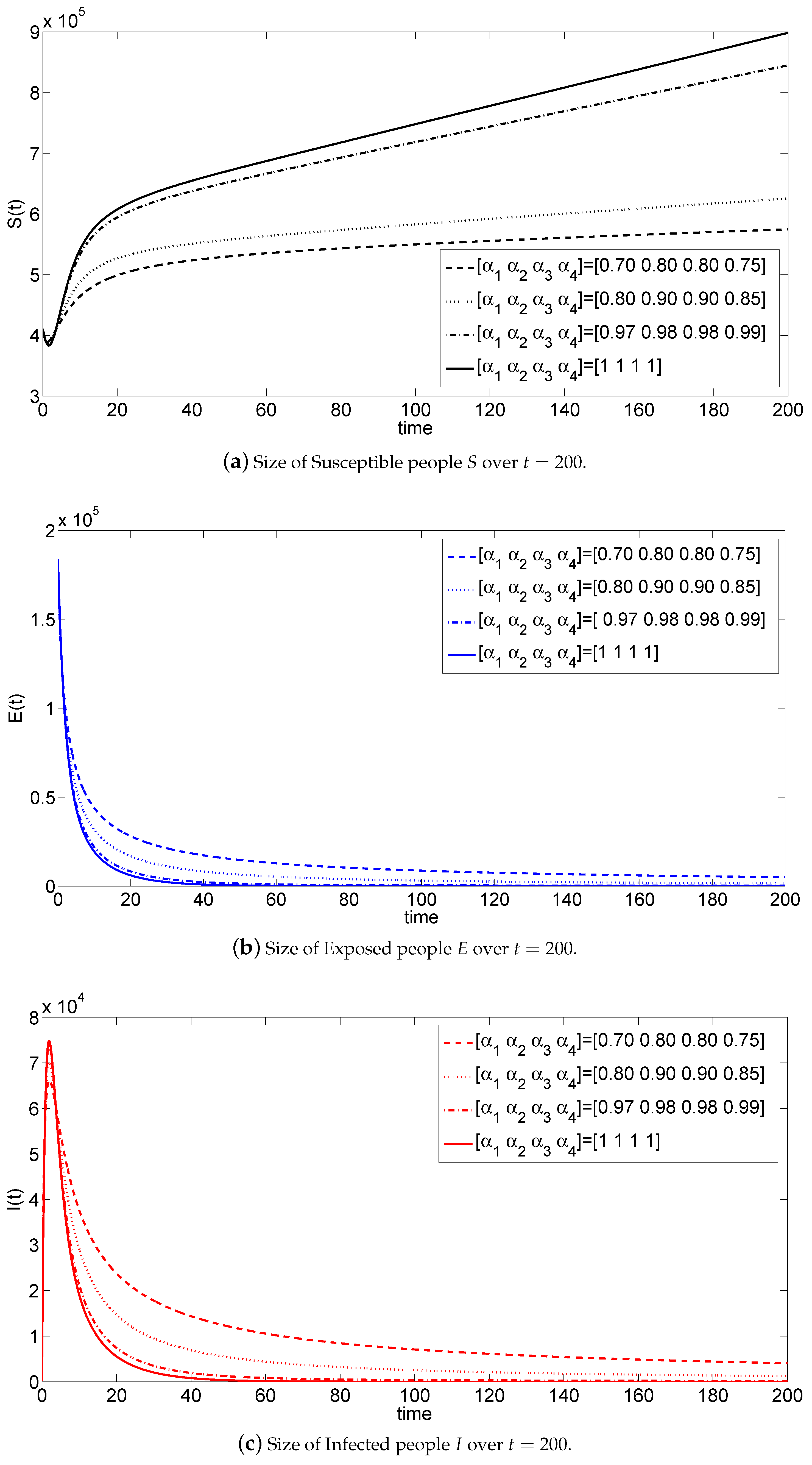
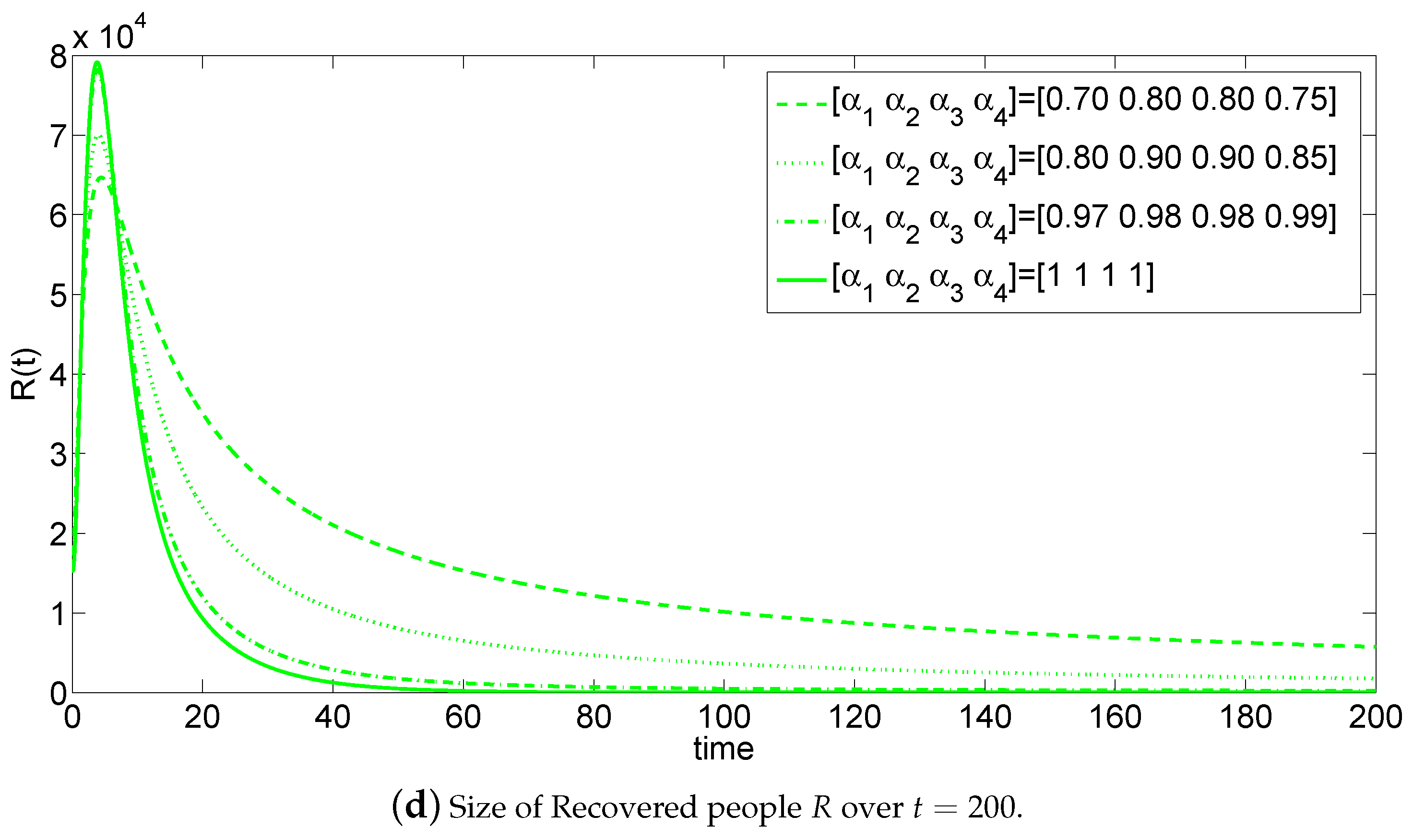
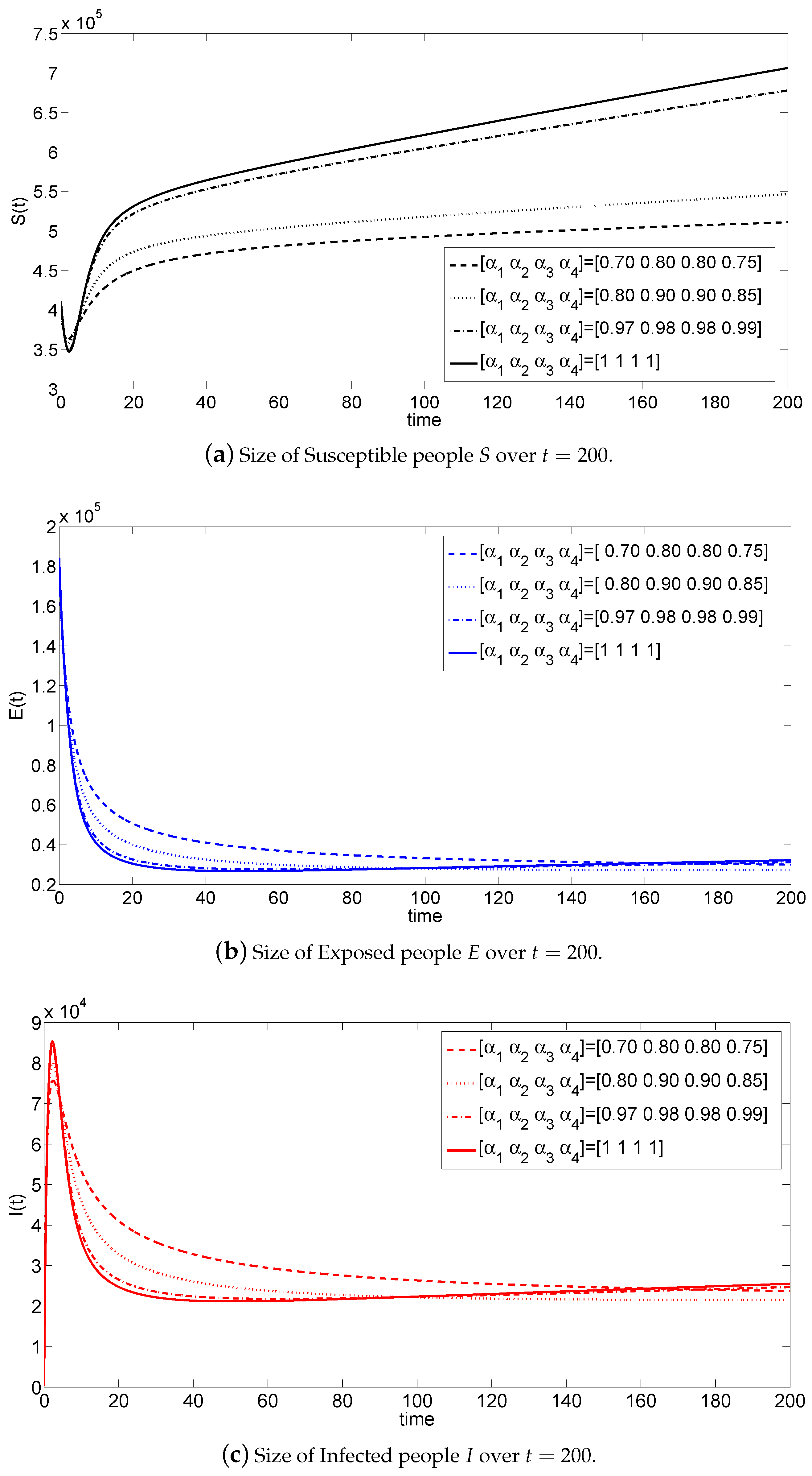
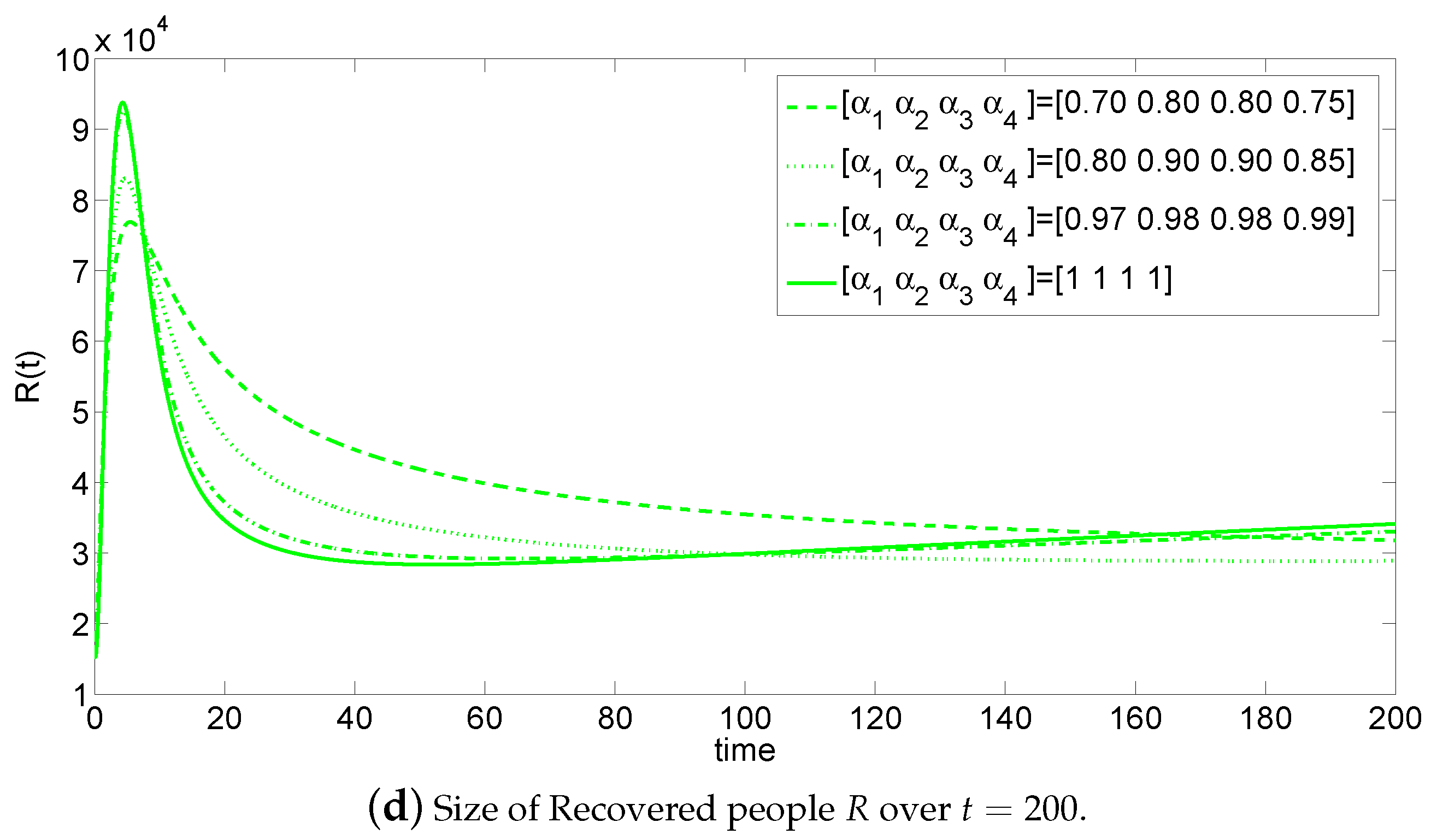
5. Numerical Simulations

In this section, we will perform several numerical simulations to verify the results mentioned in the previous section. We take the value of the initial population as $N\left(0\right)=$ 610,624, so that it is divided as follows: the number of susceptible people $S\left(0\right)=$ 410,624, the number of exposed people $E\left(0\right)=$ 183,981, the number of infected people $I\left(0\right)=267$, and the number of people who have recovered from the disease $R\left(0\right)=15,752$. In the same regard, we assume the parameters of system (3) as follows: the value of the recruitment rate into susceptible population is $\mathsf{\Lambda }=1534$, the value of the natural death rate is $\mu =3.53513\times {10}^{-5}$, the value of the rate of transmission of people from group E to group I is $\rho =0.61515$, the value of the death rate caused by the coronavirus $d=0.022801$, the value of recovery rate $\gamma =0.75217$, and the value of the rate of transmission of people from group R to group S is $\tau =0.56128$. The rate of new infections $r_1=0.40221$, which is related to the friction of group I with group S, such that it is greater than $r_2=0.24521$, which is related to the friction of group S with group I. This is because the people in group I have a visible injury, and this means that their contact with group S is small. On the other hand, we take the fractional-order values as:

$${\alpha }_1=0.7,{\alpha }_2={\alpha }_3=0.8,{\alpha }_4=0.75.$$

(46)

In order to apply Theorem 5, one should first calculate $R_0$ to be as follows:

$$\begin{array}{cc}{R}_0\hfill & =\frac{r_1(d+\gamma +\mu )+\rho r_2}{\left(\mu +\rho \right)\left(d+\gamma +\mu \right)}\hfill \\ \hfill & =\frac{0.40221(0.022801+0.75217+3.53513\times {10}^{-5})+\left(0.61515\right)\left(0.24521\right)}{\left(3.53513\times {10}^{-5}+0.61515\right)(0.022801+0.75217+3.53513\times {10}^{-5})}\hfill \\ \hfill & =0.97018.\hfill \end{array}$$

(47)

Due to $R_0<1$, the pandemic will disappear according to Theorem 5. However, according to the two values of time ($t=20$ and $t=200$ days) and according to the values of ${\alpha }_i$ ($i=1,2,3,4$) given in (46), we generate, respectively, Figure 1a,b, which represent the dynamics of system (3) in case of $R_0<1$.

In the same regard, we plot Figure 2, which represents another dynamic of system (3) but with different values of each of ${\alpha }_i$, where $i=1,2,3,4$.

In light of this figure, we notice that any change in the fractional-order values allows us to control the curvature of the curves. In other words, the incommensurate fractional-order values can allow us to control the slope of the curves separately from each other, which gives us more freedom to make a model that is more compatible with the real results.

On the other hand, if we take the value $r_1=0.50221$, we get $R_0>1$. Thus, according to $t=20$ and $t=200$ days, as well as the values of ${\alpha }_i$ ($i=1,2,3,4$) given in (46), we can generate, respectively, Figure 3a,b, which represent the dynamics of system (3) in case of $R_0>1$.

Based on these curves, we notice that the free disease fixed point is unstable. In fact, this system has another fixed point called the pandemic fixed point, in which studying its stability is deemed a very difficult mission in the abstract case due to the complexity of its calculation. However, Figure 4 shows that the free disease fixed point is also unstable and the pandemic point is asymptotic stable, according to different values of each ${\alpha }_i$, where $i=1,2,3,4$.

6. Conclusions

In this paper, several existence and uniqueness results, as well as several stability analysis results, of a new version of the $SEIR$ model established in view of incommensurate fractional-order derivatives have been investigated. It is worth mentioning that to achieve a good study of the pandemic disease, we should have correct statistics for a certain period of such disease. The longer this period is, the more accurate results of the predictions will be. Furthermore, we can conclude that, when dealing with the integer-order system, there is difficulty persuading the system to agree with certain statistics. This is because the curvature is constant, which means that the integer-order system cannot be agreed with the collected statistics. For this reason, we can use the incommensurate fractional-order models, as shown for system (3). It has been observed that any change in the fractional-order values can allow to control the curvature of the system’s curves. This, immediately, can allow us to agree between the real results and the system’s dynamics in a given interval, as previously shown in Figure 2 and Figure 4. We would then obtain more accurate predictions than that of the integer-order systems. One of the significant features here lies in the fact that when the curvature of any state of the system is changed to match the desired results, the other curvatures of the other compartments will be affected. In other words, we can make the results of any compartment of the system more accurate by controlling the curvature of each state independently, and then we can provide accurate predictions for each one. This is exactly the benefit of using the incommensurate fractional-order in the $SEIR$ models.

References

1. Wang, D.; Hu, B.; Hu, C.; Zhu, F.; Liu, X.; Zhang, J.; Wang, B.; Xiang, H.; Cheng, Z.; Xiong, Y.; et al. Clinical characteristics of 138 hospitalized patients with 2019 novel coronavirus–infected pneumonia in Wuhan, China. JAMA 2020, 323, 1061–1069. [Google Scholar] [CrossRef] [PubMed]
2. Zhu, N.; Zhang, D.; Wang, W.; Li, X.; Yang, B.; Song, J.; Zhao, X.; Huang, B.; Shi, W.; Lu, R.; et al. A novel coronavirus from patients with pneumonia in China, 2019. N. Engl. J. Med. 2020, 382, 727–733. [Google Scholar] [CrossRef] [PubMed]
3. Wintachai, P.; Prathom, K. Stability analysis of SEIR model related to efficiency of vaccines for COVID-19 situation. Heliyon 2021, 7, e06812. [Google Scholar] [CrossRef] [PubMed]
4. Xu, Z.; Shi, L.; Wang, Y.; Zhang, J.; Huang, L.; Zhang, C.; Liu, S.; Zhao, P.; Liu, H.; Zhu, L.; et al. Pathological findings of Covid-19 associated with acute respiratory distress syndrome. Lancet Respir. Med. 2020, 8, 420–422. [Google Scholar] [CrossRef]
5. Huang, C.; Wang, Y.; Li, X.; Ren, L.; Zhao, J.; Hu, Y.; Zhang, L.; Fan, G.; Xu, J.; Gu, X.; et al. Clinical features of patients infected with 2019 novel coronavirus in Wuhan, China. Lancet 2020, 395, 497–506. [Google Scholar] [CrossRef] [Green Version]
6. Guo, T.; Shen, Q.; Guo, W.; He, W.; Li, J.; Zhang, Y.; Wang, Y.; Zhou, Z.; Deng, D.; Ouyang, X.; et al. Clinical characteristics of elderly patients with Covid-19 in Hunan province, China: A multicenter, retrospective study. Gerontology 2020, 66, 467–475. [Google Scholar] [CrossRef]
7. Oreshkova, N.; Molenaar, R.J.; Vreman, S.; Harders, F.; Munnink, B.B.O.; der Honing, R.W.H.; Gerhards, N.; Tolsma, P.; Bouwstra, R.; Sikkema, R.S.; et al. SARS-CoV-2infection in farmed minks, the Netherlands, April and May 2020. Eurosurveillance 2020, 25, 2001005. [Google Scholar] [CrossRef]
8. Schlottau, K.; Rissmann, M.; Graaf, A.; Schön, J.; Sehl, J.; Wylezich, C.; Höper, D.; Mettenleiter, T.C.; Balkema-Buschmann, A.; Harder, T.; et al. Sars-CoV-2 in fruit bats, ferrets, pigs, and chickens: An experimental transmission study. Lancet Microbe 2020, 1, e218–e225. [Google Scholar] [CrossRef]
9. Kermack, W.O.; McKendrick, A.G. A contribution to the mathematical theory of epidemics. Proc. Roy. Soc. A 1927, 115, 700–721. [Google Scholar]
10. Pastor-Satorras, R.; Vespignani, A. Epidemic dynamics and endemic states in complex networks. Proc. Rev. E 2001, 63, 66117. [Google Scholar] [CrossRef] [Green Version]
11. Soper, H.E. The interpretation of periodicity in disease prevalence. J. R. Stat. Soc. 1929, 92, 34. [Google Scholar] [CrossRef]
12. Bestehorn, M.; Michelitsch, T.M.; Collet, B.A.; Riascos, A.P.; Nowakowski, A.F. Simple model of epidemic dynamics with memory effects. Phys. Rev. E 2022, 105, 24205. [Google Scholar] [CrossRef]
13. Ng, T.W.; Turinici, G.; Danchin, A. A double epidemic model for the Sars propagation. BMC Infect. Dis. 2003, 3, 19. [Google Scholar] [CrossRef]
14. Han, X.-N.; Vlas, S.J.D.; Fang, L.-Q.; Feng, D.; Cao, W.-C.; Habbema, J.D.F. Mathemat-ical modelling of Sars and other infectious diseases in China: A review. Trop. Med. Int. Health 2009, 14, 92–100. [Google Scholar] [CrossRef]
15. Kwon, C.-M.; Jung, J.U. Applying discrete SEIR model to characterizing MERSspread in Korea. Int. J. Model. Simul. Sci. Comput. 2016, 7, 1643003. [Google Scholar] [CrossRef]
16. Manaqib, M.; Fauziah, I.; Mujiyanti, M. Mathematical model for MERS-COVdisease transmission with medical mask usage and vaccination. InPrime Indones. J. Pure Appl. Math. 2019, 1, 30–42. [Google Scholar] [CrossRef]
17. Diaz, P.; Constantine, P.; Kalmbach, K.; Jones, E.; Pankavich, S. A modified SEIRmodel for the spread of Ebola in western Africa and metrics for resource allocation. Appl. Math. Comput. 2018, 324, 141–155. [Google Scholar]
18. Boujakjian, H. Modeling the spread of Ebola with SEIRand optimal control. SIAM Undergrad. Res. Online 2016, 9, 299–310. [Google Scholar] [CrossRef]
19. Syafruddin, S.; Noorani, M. SEIRmodel for transmission of Dengue fever in SelangorMalaysia. Int. J. Mod. Phys. Conf. Ser. 2012, 9, 380–389. [Google Scholar]
20. Esteva, L.; Vargas, C. Analysis of a Dengue disease transmission model. Math. Biosci. 1998, 150, 131–151. [Google Scholar] [CrossRef]
21. Sungchasit, R.; Pongsumpun, P. Mathematical model of Dengue virus with primary and secondary infection. Curr. Appl. Sci. Technol. 2019, 19, 154–176. [Google Scholar]
22. Albadarneh, R.B.; Batiha, I.M.; Ouannas, A.; Momani, S. Modeling COVID-19 Pandemic Outbreak using Fractional-Order Systems. Int. J. Math. Comput. Sci. 2021, 16, 1405–1421. [Google Scholar]
23. Almatroud, A.O.; Djenina, N.; Ouannas, A.; Grassi, G.; Al-sawalha, M.M. A novel discrete-time COVID-19 epidemic model including the compartment of vaccinated individuals. Math. Biosci. Eng. 2022, 19, 12387–12404. [Google Scholar] [CrossRef] [PubMed]
24. Dababneh, A.; Djenina, N.; Ouannas, A.; Grassi, G.; Batiha, I.M. A New Incommensurate Fractional-Order Discrete COVID-19 Model with Vaccinated Individuals Compartment. Fractal Fract. 2022, 6, 456. [Google Scholar] [CrossRef]
25. Abbes, A.; Ouannas, A.; Shawagfeh, N.; Jahanshahi, H. The fractional-order discrete COVID-19 pandemic model: Stability and chaos. Nonlinear Dyn. 2023, 111, 965–983. [Google Scholar] [CrossRef]
26. Djenina, N.; Ouannas, A.; Batiha, I.M.; Grassi, G.; Oussaeif, T.E.; Momani, S. A novel fractional-order discrete SIR model for predicting COVID-19 behavior. Mathematics 2022, 10, 2224. [Google Scholar] [CrossRef]
27. Momani, S.; Ouannas, A.; Momani, Z.; Hadid, S.B. Fractional-order COVID-19 pandemic outbreak: Modeling and stability analysis IM Batiha. Int. J. Biomath. 2022, 15, 2150090. [Google Scholar]
28. Djenina, N.; Ouannas, A. The fractional discrete model of COVID-19: Solvability and simulation. Innov. J. Math. 2022, 1, 23–33. [Google Scholar] [CrossRef]
29. Batiha, I.; Al-Nana, A.A.; Albadarneh, R.B.; Ouannas, A.; Al-Khasawneh, A.; Momani, S. Fractional-order coronavirus models with vaccination strategies impacted on Saudi Arabia’s infections. AIMS Math. 2022, 7, 12842–12858. [Google Scholar] [CrossRef]
30. Debbouche, N.; Ouannas, A.; Batiha, I.M.; Grassi, G. Chaotic dynamics in a novel COVID-19 pandemic model described by commensurate and incommensurate fractional-order derivatives. Nonlinear Dyn. 2022, 109, 1–13. [Google Scholar] [CrossRef]
31. Chicchi, L.; Patti, F.D.; Fanelli, D.; Piazza, F.; Ginelli, F. First results with a SEIRD model: Quantifying the population of asymptomatic individuals in Italy, Preprint, Part of the project Analysis and forecast of COVID-19 spreading. 2020. [Google Scholar]
32. Samko, S.G.; Kilbas, A.A.; Marichev, O.I. Fractional Integrals and Derivatives: Theory and Applications; Gordon and Breach Science Publishers: Basel, Switzerland, 1993. [Google Scholar]
33. Odibat, Z.M.; Shawagfeh, N.T. Generalized Taylor’s formula. Appl. Math. Comput. 2007, 186, 286–293. [Google Scholar] [CrossRef]
34. Li, Y.; Chen, Y.; Podlubny, I. Stability of fractional-order nonlinear dynamic systems: Lyapunov direct method and generalized Mittag Leffler stability. Comput. Math. Appl. 2010, 59, 1810–1821. [Google Scholar] [CrossRef]
Figure 1. The dynamics of system (3) according to the values of α reported in (46) and in case of R 0 < 1 .
Mathematics 11 00555 g001
Figure 2. Size of all classes for system (3) according to different values of α and in case of R 0 < 1 .
Mathematics 11 00555 g002aMathematics 11 00555 g002b
Figure 3. The dynamics of system (3) according to the values of α reported in (46) and in case of R 0 > 1 .
Mathematics 11 00555 g003
Figure 4. Size of all classes for system (3) according to different values of α and in case of R 0 > 1 .
Mathematics 11 00555 g004aMathematics 11 00555 g004b