Hopf Bifurcation in a Predator–Prey Model with Memory Effect in Predator and Anti-Predator Behaviour in Prey

Abstract

In this paper, a diffusive predator–prey model with a memory effect in predator and anti-predator behaviour in prey is studied. The stability of the coexisting equilibrium and the existence of Hopf bifurcation are analysed by analysing the distribution of characteristic roots. The property of Hopf bifurcation is investigated by the theory of the centre manifold and normal form method. Through the numerical simulations, it is observed that the anti-predator behaviour parameter $\eta$, the memory-based diffusion coefficient parameter d, and memory delay $\tau$ can affect the stability of the coexisting equilibrium under some parameters and cause the spatially inhomogeneous oscillation of prey and predator’s densities.

1. Introduction

The predator–prey model has attracted the attention of many scholars [1,2,3]. Traditional predator–prey models often label animals as predator and prey; this is based on the assumptions that predators feed on prey [4,5,6]. However, sometimes, anti-predator behaviour in prey may occur [7,8]. Experiments show that anti-predator behaviour in prey can be divided into two cases [9]: (a) morphological changes or through changes in behaviour [10,11] or (b) the preys attack their predators [12,13].

B. Tang and Y. Xiao [9] proposed the following model:

$$\begin{array}{c}\hfill \left\{\begin{array}{c}\frac{du}{dt}=ru(1-\frac{u}{K})-\frac{\beta uv}{a+u^2},\hfill \\ \frac{dv}{dt}=\frac{\mu \beta uv}{a+u^2}-cv-\eta uv.\hfill \end{array}\right.\end{array}$$

(1)

All the parameters are positive. r, K, $\beta$, a, $\mu$, and c represent the growth rate, carrying capacity, capture rate, handling time, conversion rate, and death rate, respectively. The term $\eta uv$ represents the anti-predator behaviour in prey. The function response $\frac{\beta u}{a+u^2}$ is the simplified Monod–Haldane function, which is also called the Holling type IV functional response. They mainly studied the bifurcations, including saddle–node bifurcation, Hopf bifurcation, homoclinic bifurcation, and a Bogdanov–Takens bifurcation of codimension 2, and showed that anti-predator behaviour is a benefit for the prey population [9].

Motivated by the work of [9], some scholars have studied the predator–prey models using anti-predator behaviour [14,15,16,17]. Wang et al. studied a predator–prey model with a stage structure for the prey and anti-predator behaviour and mainly focused on the stability and Hopf bifurcation [15]. J. Liu and X. Zhang considered a delayed reaction–diffusion predator–prey model with anti-predator behaviour and a Holling II functional response [16]. They mainly studied the Turing instability and Hopf bifurcation. R. Yang and J. Ma studied a diffusive predator–prey model with anti-predator behaviour and a Beddington–DeAngelis functional response and showed that the Turing instability induced by diffusion and Hopf bifurcation were induced by time delay [17]. Although it is shown in the literature [16,17] that there may be spatially inhomogeneous periodic solutions caused by time delay, no examples of spatially inhomogeneous periodic solutions are provided in numerical simulations.

In the real world, prey and predators are not static in space and they often engender self-diffusion. Therefore, many scholars use a reaction diffusion equation to describe the growth law of populations [18,19]. In addition, smart predators also have memory effect and cognitive behaviour [20]. For example, blue whales migrate by memory. Another example is that animals in polar regions usually determine their spatial movement by judging their footprints, which record the history of species’ distributions and movements, including time delay. Obviously, highly developed animals can even remember their historical distribution or cluster of species in space. Great progress has been made in the implicit integration of spatial cognition or memory [21,22,23]. Some scholars have studied spatial memory in population models by introducing an additional delayed diffusion term [24,25,26]. In [22], the authors studied a memory-based reaction–diffusion equation with nonlocal maturation delay and a homogeneous Dirichlet boundary condition and mainly considered the local stability and Hopf bifurcation. In [25], Song et al. provided a normal form theory for Turing–Hopf bifurcation in the general reaction–diffusion equation with memory-based diffusion and a nonlocal reaction. In [26], Song et al. obtained the normal form of the Hopf bifurcation in the predator–prey model with a memory effect.

In this paper, assuming the predator has spatial-memory diffusion, we study the following model:

$$\left\{\begin{array}{c}\frac{\partial u(x,t)}{\partial t}=d_1\Delta u+ru(1-\frac{u}{K})-\frac{\beta uv}{a+u^2},\hfill \\ \frac{\partial v(x,t)}{\partial t}=-d\nabla (v\nabla u(t-\tau ))+d_2\Delta v+\frac{\mu \beta uv}{a+u^2}-cv-\eta uv,x\in \mathrm{\Omega },t>0\hfill \\ \frac{\partial u(x,t)}{\partial \overline{\nu }}=\frac{\partial v(x,t)}{\partial \overline{\nu }}=0,x\in \partial \mathrm{\Omega },t>0\hfill \\ u(x,\theta )=u_0(x,\theta )\ge 0,v(x,\theta )=v_0(x,\theta )\ge 0,x\in \overline{\mathrm{\Omega }},\theta \in [-\tau ,0].\hfill \end{array}\right.$$

(2)

where $d_1$ and $d_2$ are self-diffusion parameters. The term $-d\nabla (v\nabla u(t-\tau \left)\right)$ is the memory-based diffusion effect. d is the memory-based diffusion co-efficient and the time delay $\tau >0$ is the averaged memory period of the predator. If we assume the region the prey and predator live in is closed, then the Neumann boundary condition is used. For the convenience of calculation, we use $\mathrm{\Omega }=(0,l\pi )$. As far as we know, no one has studied the model (2) at present. The aim of this paper is to study the effect of the memory delay, the memory-based diffusion, and the anti-predator behaviour on the model (2) from the perspective of stability and Hopf bifurcation.

The paper is arranged as follows. In Section 2, we studied the stability and the existence of Hopf bifurcation. In Section 3, we analysed the property of Hopf bifurcation. In Section 4, we provide some numerical simulations. In Section 5, we obtain a short conclusion.

2. Stability Analysis

The existence of equilibria has been studied in [9]. For the sake of completeness, we just provide the following lemma; the proof is available in [9].

Lemma 1. 

The existence of equilibria for model (2) is as follows.

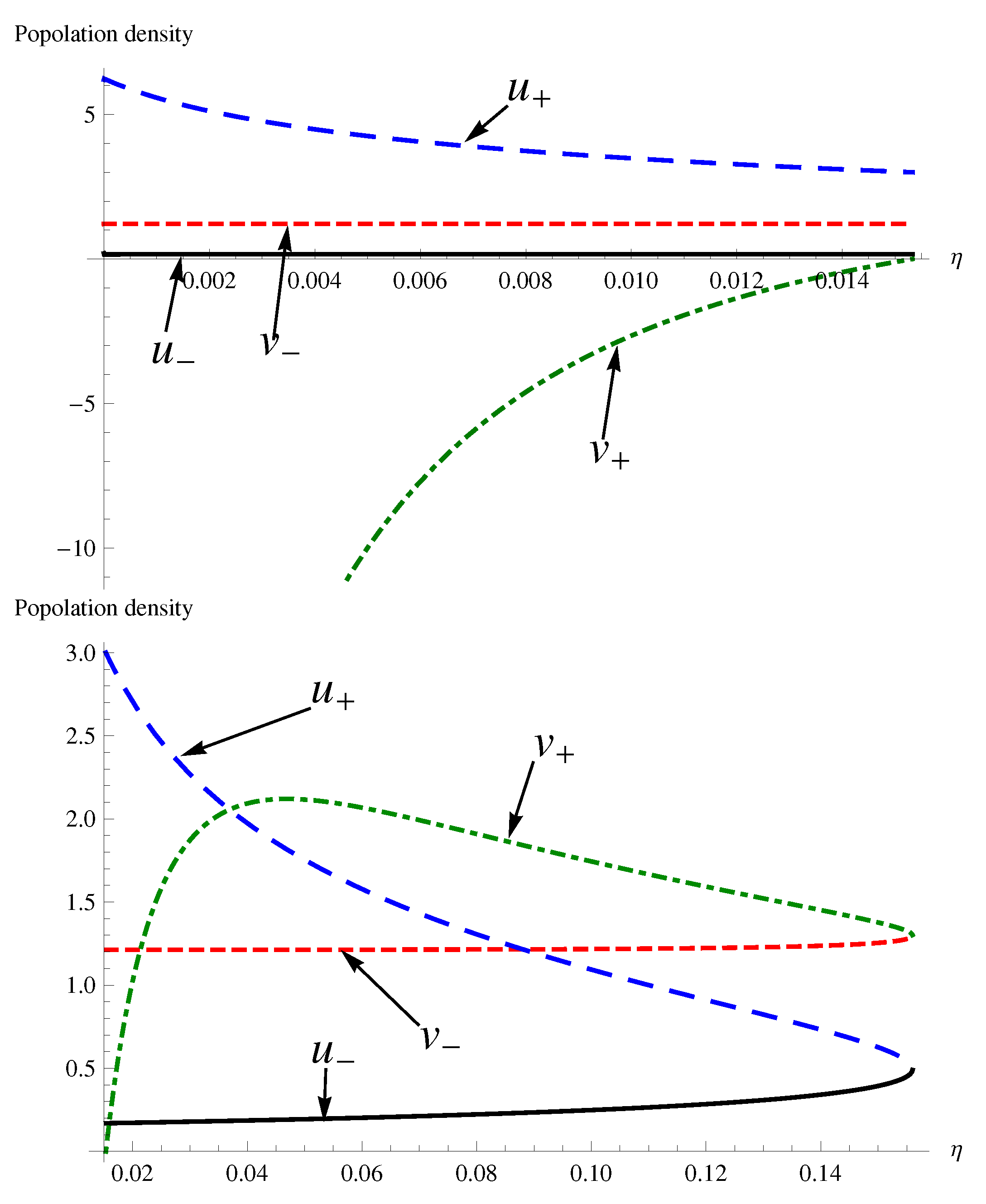
• The model (2) always has two boundary equilibriums $(0,0)$ and $(K,0)$.
• Case I: $a\eta -\beta \mu \ge 0$. The model (2) always has no positive equilibrium.
• Case II: $a\eta -\beta \mu <0$.

  ★

  Subcase I: The model (2) always has no positive equilibrium when $f\left(u_c\right)>0$.

  ★

  Subcase II: The model (2) has two positive equilibria $(u_{-},v_{-})$ and $(u_{+},v_{+})$ when $f\left(u_c\right)<0$ and $f\left(K\right)>0$.

  ★

  Subcase III: The model (2) has a unique positive equilibrium $(u_{-},v_{-})$ when $f\left(u_c\right)<0$ and $f\left(K\right)\le 0$.

  ★

  Subcase IV: The model (2) has a unique positive equilibrium $(u_{-},v_{-})$=$(u_{+},v_{+})$ when $f\left(u_c\right)=0$.

where $u_c=\frac{-c+\sqrt{c^2-3\eta (a\eta -\beta \mu )}}{3\eta },$$f\left(u_c\right)=\frac{1}{27{\eta }^2}\left(2c^3+9c\eta (2a\eta +\beta \mu )-2{\left(c^2+3\eta (-a\eta +\beta \mu )\right)}^{3/2}\right)$, $f\left(u\right)=u^3\eta +c{u}^2+u(a\eta -\beta \mu )+ac=0$, $u_{\pm }=\frac{-c+\sqrt{A}\left(\cos \left[\frac{\theta }{3}\right]\pm \sqrt{3}\sin \left[\frac{\theta }{3}\right]\right)}{3\eta }$, $v_{\pm }=\frac{r(K-u_{\pm })\left(a+u_{\pm }^2\right)}{K\beta }$, $A=c^2-3\eta (\eta a-\beta \mu )$, $B=c(\eta a-\beta \mu )-9\eta ac$, $T=\frac{(2Ac-3\eta B)}{2\sqrt{A^3}}$, $\theta =\arccos \left[T\right]$.

In the following, we just assume the model (2) has a positive equilibrium $E_{*}(u_{*},v_{*})$. In particular, the model (2) may have two positive equilibria. Then, we can use the same method to study the property for different positive equilibria. The linear system of (2) at $E_{*}(u_{*},v_{*})$ is

$$\frac{\partial u}{\partial t}\left(\begin{array}{c}u(x,t)\hfill \\ u(x,t)\hfill \end{array}\right)=J_1\left(\begin{array}{c}\Delta u\left(t\right)\hfill \\ \Delta v\left(t\right)\hfill \end{array}\right)+J_2\left(\begin{array}{c}\Delta u(t-\tau )\hfill \\ \Delta v(t-\tau )\hfill \end{array}\right)+L\left(\begin{array}{c}u(x,t)\hfill \\ v(x,t)\hfill \end{array}\right),$$

(3)

where

$$J_1=\left(\begin{array}{cc}{d}_1& 0\\ 0& d_2\end{array}\right),J_2=\left(\begin{array}{cc}0& 0\\ -d{v}_{*}& 0\end{array}\right),L=\left(\begin{array}{cc}{\alpha }_1& {\alpha }_2\\ {\beta }_1& 0\end{array}\right),$$

and ${\alpha }_1=-\frac{r{u}_{*}}{K\left(a+u_{*}^2\right)}\left(a-2K{u}_{*}+3u_{*}^2\right)$, ${\alpha }_2=-\frac{u_{*}\beta }{a+u_{*}^2}<0$, ${\beta }_1=v_{*}\left(\frac{\left(a-u_{*}^2\right)\beta \mu }{{\left(a+u_{*}^2\right)}^2}-\eta \right)$.

The characteristic equations are:

$${\lambda }^2+{\kappa }_n\lambda +{\nu }_n+{\varrho }_n{e}^{-\lambda \tau }=0,n\in {\mathbb{N}}_0,$$

(4)

where

$${\kappa }_n=(d_1+d_2){\mu }_n-{\alpha }_1,{\nu }_n=-{\alpha }_2{\beta }_1-{\alpha }_1{d}_2{\mu }_n+d_1{d}_2{\mu }_n^2,{\varrho }_n=-{\alpha }_{2}d{v}_{*}{\mu }_n,{\mu }_n=\frac{n^2}{l^2}.$$

2.1. $\tau =0$

The characteristic Equations (4) are:

$${\lambda }^2+{\kappa }_n\lambda +{\nu }_n+{\varrho }_n=0,n\in {\mathbb{N}}_0,$$

(5)

where ${\nu }_n+{\varrho }_n=-{\alpha }_2{\beta }_1-({\alpha }_{2}d{v}_{*}+{\alpha }_1{d}_2){\mu }_n+d_1{d}_2{\mu }_n^2$. We propose the following hypothesis:

Hypothesis 1 (H1).

$$a\eta -\beta \mu <0,K<\frac{a+3u_{*}^2}{2u_{*}},\eta <\frac{\left(a-u_{*}^2\right)\beta \mu }{{\left(a+u_{*}^2\right)}^2}.$$

In particular, in (H1), $K<\frac{a+3u_{*}^2}{2u_{*}}$ implies ${\alpha }_1<0$, and $\eta <\frac{\left(a-u_{*}^2\right)\beta \mu }{{\left(a+u_{*}^2\right)}^2}$ implies ${\beta }_1>0$. We should notice that $u_{*}$ is related to parameter $\eta$, so $\eta <\frac{\left(a-u_{*}^2\right)\beta \mu }{{\left(a+u_{*}^2\right)}^2}$ is very complicated. Then we can obtain the following theorem.

Theorem 1. 

For system (2) with $\tau =0$, $E_{*}(u_{*},v_{*})$ is locally stable under (H1).

2.2. $\tau >0$

Assume (H1) holds and let $i\omega$ ($\omega >0$) be a solution of (4), then:

$$-{\omega }^2+{\kappa }_n\mathrm{i}\omega +{\nu }_n+{\varrho }_n(\cos \omega \tau -\mathrm{i}\sin \omega \tau )=0.$$

We can obtain $\cos \omega \tau =\frac{{\omega }^2-{\nu }_n}{{\varrho }_n}$, $\sin \omega \tau =\frac{{\kappa }_n\omega }{{\varrho }_n}>0$ under hypothesis (H1). It leads to:

$${\omega }^4+\left({\kappa }_n^2-2{\nu }_n\right){\omega }^2+{\nu }_n^2-{\varrho }_n^2=0.$$

(6)

Let $p={\omega }^2$, then (6) becomes:

$$p^2+\left({\kappa }_n^2-2{\nu }_n\right)p+{\nu }_n^2-{\varrho }_n^2=0,$$

(7)

and the roots of (7) are $p_n^{\pm }=\frac{1}{2}[-\left({\kappa }_n^2-2{\nu }_n\right)\pm \sqrt{{\left({\kappa }_n^2-2{\nu }_n\right)}^2-4({\nu }_n^2-{\varrho }_n^2)}].$ By direct computation, we have:

$$\left\{\begin{array}{cc}\hfill {\kappa }_n^2-2{\nu }_n& =(d_1^2+d_2^2){\mu }_n^2-2{\alpha }_1{d}_1{\mu }_n+{\alpha }_1^2+2{\alpha }_2{\beta }_1,\hfill \\ \hfill {\nu }_n-{\varrho }_n& =d_1{d}_2\frac{n^4}{l^4}+({\alpha }_{2}d{v}_{*}-{\alpha }_1{d}_2){\mu }_n-{\alpha }_2{\beta }_1,\hfill \end{array}\right.$$

and ${\nu }_n+{\varrho }_n>0$ under hypothesis (H1). Define ${\eta }_{\pm }=\frac{-({\alpha }_{2}d{v}_{*}-{\alpha }_1{d}_2)\pm \sqrt{{({\alpha }_{2}d{v}_{*}-{\alpha }_1{d}_2)}^2-4d_1{d}_2(-{\alpha }_2{\beta }_1)}}{2d_1{d}_2}$, $d_{*}=\frac{{\alpha }_1{d}_2}{{\alpha }_2{v}_{*}}+\frac{2}{v_{*}}\sqrt{-\frac{b_1{d}_1{d}_2}{{\alpha }_2}}$, and $\mathbb{S}=\left\{n\right|\frac{n^2}{l_2}\in ({\eta }_{-},{\eta }_{+}),n\in {\mathbb{N}}_0\}$. Then:

$$\left\{\begin{array}{c}{\nu }_n-{\varrho }_n>0,ford\le d_{*},n\in {\mathbb{N}}_0,\hfill \\ {\nu }_n-{\varrho }_n>0,ford>d_{*},n\notin \mathbb{S},\hfill \\ {\nu }_n-{\varrho }_n<0,ford>d_{*},n\in \mathbb{S}.\hfill \end{array}\right.$$

(8)

The existence of purely imaginary roots of Equation (4) can be divided into the following two cases.

Case 1:${\alpha }_1^2+2{\alpha }_2{\beta }_1>0$. We can obtain ${\kappa }_n^2-2{\nu }_n>{\alpha }_1^2+2{\alpha }_2{b}_1>0$. For $d>d_{*}$ and $n\in \mathbb{S}$, then Equation (4) has a pair of purely imaginary roots $\pm i{\omega }_n^{+}$ at ${\tau }_n^{j,+}$ for $j\in {\mathbb{N}}_0$ and $n\in \mathbb{S}$. Otherwise, Equation (4) does not have characteristic roots with zero real parts.

Case 2:${\alpha }_1^2+2{\alpha }_2{\beta }_1<0$. Divide this case into the following two subcases.

• For $d\le d_{*}$ and $n\in {\mathbb{S}}_1:=\left\{n\right|{\kappa }_n^2-2{\nu }_n<0,{\left({\kappa }_n^2-2{\nu }_n\right)}^2-4({\nu }_n^2-{\varrho }_n^2)>0,n\in {\mathbb{N}}_0\}$, then Equation (4) has two pairs of purely imaginary roots $\pm i{\omega }_n^{\pm }$ at ${\tau }_n^{j,\pm }$ for $j\in {\mathbb{N}}_0$ and $n\in {\mathbb{S}}_1$. Otherwise, Equation (4) does not have characteristic roots with zero real parts.
• For $d>d_{*}$ and $n\in {\mathbb{S}}_2:=\left\{n\right|{\kappa }_n^2-2{\nu }_n<0,{\left({\kappa }_n^2-2{\nu }_n\right)}^2-4({\nu }_n^2-{\varrho }_n^2)>0,n\in {\mathbb{N}}_0,n\notin \mathbb{S}\}$, then Equation (4) has two pairs of purely imaginary roots $\pm i{\omega }_n^{\pm }$ at ${\tau }_n^{j,\pm }$ for $j\in {\mathbb{N}}_0$ and $n\in {\mathbb{S}}_1$. For $d>d_{*}$ and $n\in \mathbb{S}$, then Equation (4) has a pair of purely imaginary roots $\pm i{\omega }_n^{+}$ at ${\tau }_n^{j,+}$ for $j\in {\mathbb{N}}_0$ and $n\in \mathbb{S}$. Otherwise, Equation (4) does not have characteristic roots with zero real parts.

Where

$${\omega }_n^{\pm }=\sqrt{p_n^{\pm }},{\tau }_n^{j,\pm }=\frac{1}{{\omega }_n^{\pm }}\arccos \left(\frac{{\left({\omega }_n^{\pm }\right)}^2-{\nu }_n}{{\varrho }_n}\right)+2j\pi .$$

(9)

Define $\mathbb{M}=\left\{{\tau }_n^{j,+}\mathrm{or}{\tau }_n^{j,-}\right|$. Equation (4) has purely imaginary roots $\pm i{\omega }_n^{+}\mathrm{or}\pm i{\omega }_n^{-}$ when $\tau ={\tau }_n^{j,+}\mathrm{or}{\tau }_n^{j,-}\}.$

Lemma 2. 

Assume (H1) holds. Then, $Re\left(\frac{d\lambda }{d\tau }\right){|}_{\tau ={\tau }_n^{j,+}}>0$, $Re\left(\frac{d\lambda }{d\tau }\right){|}_{\tau ={\tau }_n^{j,-}}<0$ for ${\tau }_n^{j,\pm }\in \mathbb{S}$ and $j\in {\mathbb{N}}_0$.

Proof. 

By (4), we have:

$${\left(\frac{d\lambda }{d\tau }\right)}^{-1}=\frac{2\lambda +{\kappa }_n}{{\varrho }_n\lambda e^{-\lambda \tau }}-\frac{\tau }{\lambda }.$$

Then:

$$\begin{array}{cc}\hfill {\left[\mathrm{Re}{\left(\frac{d\lambda }{d\tau }\right)}^{-1}\right]}_{\tau ={\tau }_n^{j,\pm }}& =\mathrm{Re}{[\frac{2\lambda +{\kappa }_n}{{\varrho }_n\lambda e^{-\lambda \tau }}-\frac{\tau }{\lambda }]}_{\tau ={\tau }_n^{j,\pm }}\hfill \\ \hfill & ={\left[\frac{1}{{\kappa }_n^2{\omega }^2+{({\nu }_n-\omega )}^2}(2{\omega }^2+{\kappa }_n^2-2{\nu }_n)\right]}_{\tau ={\tau }_n^{j,\pm }}\hfill \\ \hfill & =\pm {\left[\frac{1}{{\kappa }_n^2{\omega }^2+{({\nu }_n-\omega )}^2}\sqrt{{({\kappa }_n^2-2{\nu }_n)}^2-4({\nu }_n^2-{\varrho }_n^2)}\right]}_{\tau ={\tau }_n^{j,\pm }}.\hfill \end{array}$$

Therefore, $\mathrm{Re}\left(\frac{d\lambda }{d\tau }\right){|}_{\tau ={\tau }_n^{j,+}}>0$, $\mathrm{Re}\left(\frac{d\lambda }{d\tau }\right){|}_{\tau ={\tau }_n^{j,-}}<0$. □

Denote ${\tau }_{*}=min\left\{{\tau }_n^{0,\pm }\right|{\tau }_n^{0,\pm }\in \mathbb{M}\}$.

Theorem 2. 

For the model (2), assume (H1) holds.

• $E_{*}(u_{*},v_{*})$ is locally stable for $\tau >0$ when $\mathbb{M}=⌀$.
• $E_{*}(u_{*},v_{*})$ is locally stable for $\tau \in [0,{\tau }_{*})$ when $\mathbb{M}\ne ⌀$.
• $E_{*}(u_{*},v_{*})$ is unstable for $\tau \in ({\tau }_{*},{\tau }_{*}+ϵ)$ for some $ϵ>0$ when $\mathbb{M}\ne ⌀$.
• $\tau ={\tau }_n^{j,+}$$(\tau ={\tau }_n^{j,-})$, $j\in {\mathbb{N}}_0$, ${\tau }_n^{j,\pm }\in \mathbb{M}$ are Hopf bifurcation points.

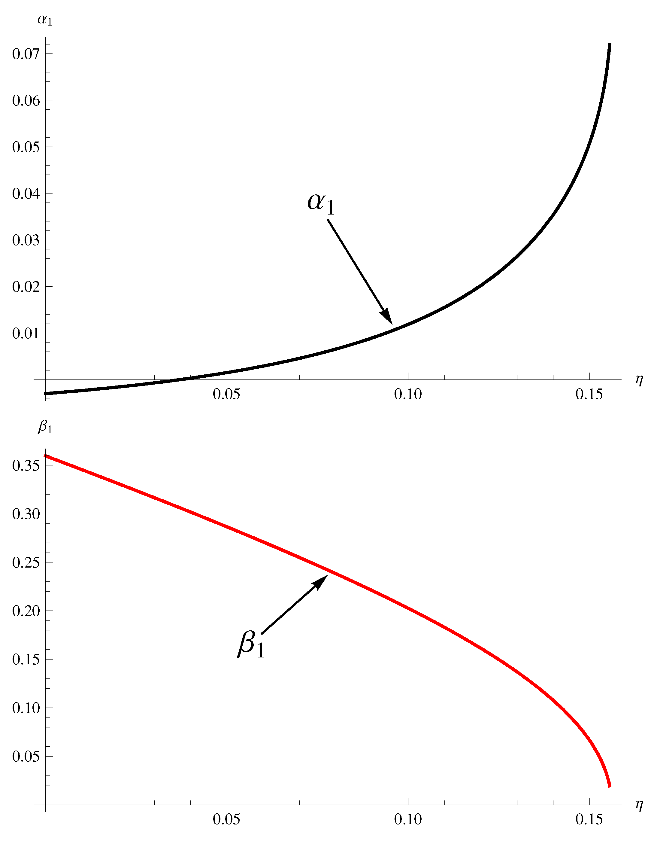
3. Property of Hopf Bifurcation

By the algorithm in [26], we provide the normal form of Hopf bifurcation as follows. The detail computation is provided in Appendix A.

$$\dot{z}=Bz+\frac{1}{2}\left(\begin{array}{c}{B}_1{z}_1\epsilon \\ {\overline{B}}_1{z}_2\epsilon \end{array}\right)+\frac{1}{3!}\left(\begin{array}{c}{B}_2{z}_1^2{z}_2\epsilon \\ {\overline{B}}_2{z}_1{z}_2^2\epsilon \end{array}\right)+O\left(\right|z|{\epsilon }^2+|z^4\left|\right),$$

(10)

where

$$B_1=2i\tilde{\omega }{\psi }^T\varphi ,B_2=B_{21}+\frac{3}{2}(B_{22}+B_{23}).$$

By coordinate transformation $z_1={\omega }_1-i{\omega }_2$, $z_2={\omega }_1+i{\omega }_2$, and ${\omega }_1=\rho \cos \xi$, ${\omega }_2=\rho \sin \xi$, the normal form (10) can be rewritten as:

$$\dot{\rho }=K_1\epsilon \rho +K_2{\rho }^3+O(\rho {\epsilon }^2+{\left|(\rho ,\epsilon )\right|}^4),$$

(11)

where $K_1=\frac{1}{2}\mathrm{Re}\left(B_1\right)$, $K_2=\frac{1}{3!}\mathrm{Re}\left(B_2\right)$.

From [26], we have the following theorem:

Theorem 3. 

If $K_1{K}_2<0(>0)$, the Hopf bifurcation is supercritical (subcritical) and the bifurcating periodic solutions is stable (unstable) for $K_2<0(>0)$.

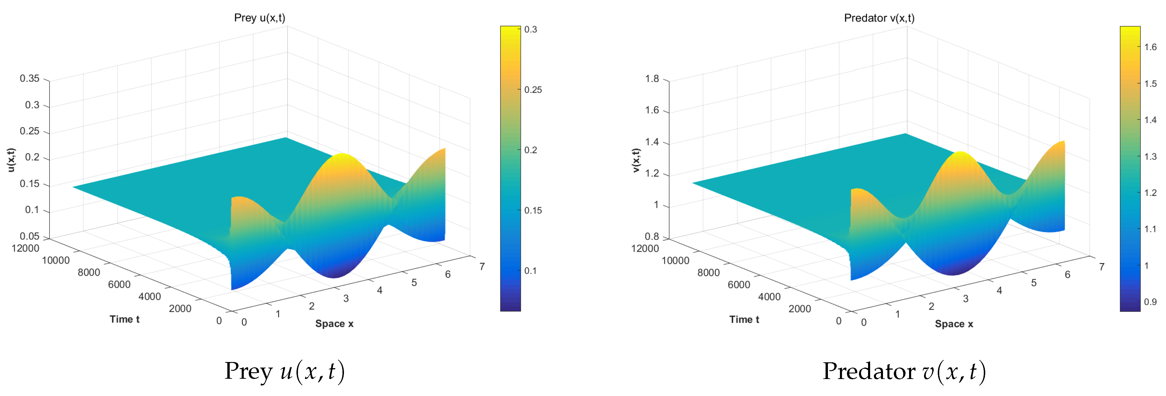
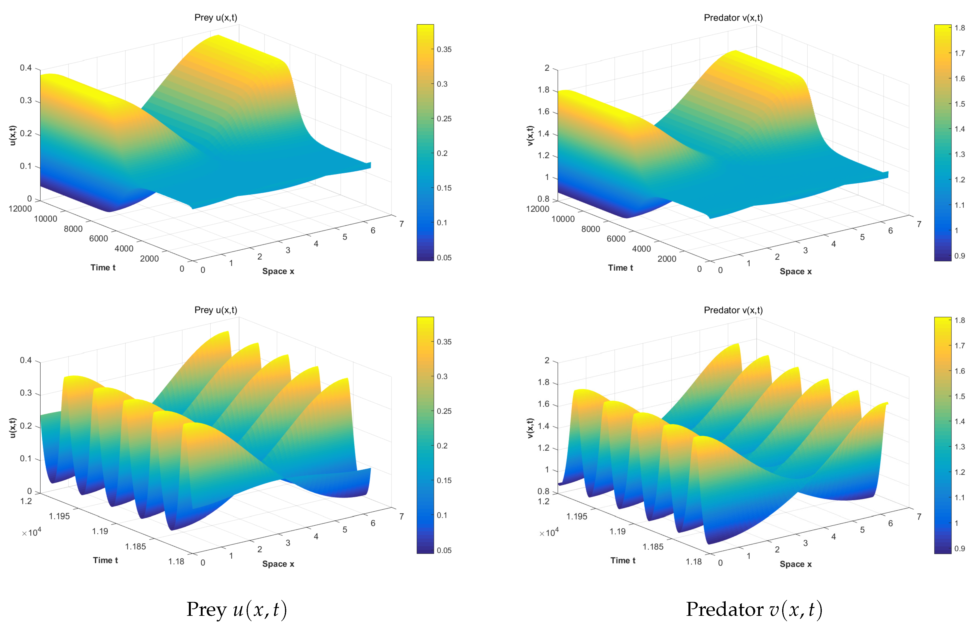
4. Numerical Simulations

Fix the following parameters:

$$c=0.05,r=0.5,a=1,\mu =0.8,\beta =0.4,K=3,d_1=0.1,d_2=0.2,l=2.$$

(12)

4.1. The Effect of Anti-Predator Behaviour

We know that the system (2) has a positive equilibrium when $\eta \le 0.1560$. Especially, the system (2) has a unique positive equilibrium $(u_{-},v_{-})$ when $\eta \le 0.0153$ (Figure 1 left) and has two positive equilibria, $(u_{-},v_{-})$ and $(u_{+},v_{+})$, when $0.0153<\eta <0.1560$ (Figure 1 right). However, when $\eta \approx 0.1560$, $(u_{-},v_{-})$ and $(u_{+},v_{+})$ coincide into one positive equilibrium (Figure 1 right).

Through analysis, we can obtain $(u_{+},v_{+})$, which is always unstable when it exists. Then, we mainly study the dynamics at $(u_{-},v_{-})$. The parameters ${\alpha }_1$ and ${\beta }_1$ with parameter $\eta$ at $(u_{-},v_{-})$ are provided in Figure 2. It shows that $(u_{-},v_{-})$ is always unstable when $\tau =0$ and anti-predator behaviour parameter $\eta$ is larger than some critical value. To guarantee assumption $\left({\mathbf{H}}_{\mathbf{1}}\right)$ is true, ${\alpha }_1<0$ and ${\beta }_1>$ should hold.

The bifurcation diagram of system (2) with parameter $\eta$ when $d=0.7$ is provided in Figure 3 left. When parameter $\eta$ increases, the stability interval of $(u_{-},v_{-})$ becomes smaller. This implies that increasing the anti-predator behaviour parameter $\eta$ is not beneficial to the uniform distribution of predator and prey and will cause inhomogeneous oscillations of the population’s density.

4.2. The Effect of Memory-Based Diffusion

We also provide the bifurcation diagram of system (2) with parameter d when $\eta =0.01$ (Figure 3 right). When parameter $d<d_{*}$, $(u_{-},v_{-})$ is always stable. When we increase parameter d until $d>d_{*}$, the Hopf bifurcating curves emerge. When parameter d increases, the stability interval of $(u_{-},v_{-})$ becomes smaller. This implies that increasing the memory-based diffusion coefficient parameter d is not beneficial to the uniform distribution of predators and prey when $d>d_{*}$ and will cause spatial oscillations of the population’s density.

4.3. The Effect of Memory Delay

Especially, we choose $\eta =0.01$, then $(u_{-},v_{-})\approx (0.1658,1.2134)$ is the unique positive equilibrium. From direct calculation, we have ${\alpha }_1^2+2{\alpha }_2{\beta }_1\approx -0.0446<0$, and $d_{*}\approx 0.5452$. Choose $d=0.7>d_{*}$, then ${\mathbb{S}}_2=\left\{1\right\}$, $\mathbb{S}=\left\{2\right\}$, ${\tau }_{*}={\tau }_1^{0,+}\approx 7.3983<{\tau }_2^{0,+}\approx 10.0126<{\tau }_1^{0,-}\approx 21.1518$ and $K_1\approx 0.04689>0$, $K_2\approx -0.0708<0$. Then $(u_{-},v_{-})$ is locally stable when $\tau \in [0,{\tau }_{*})$ (Figure 4) and unstable when $\tau >{\tau }_{*}$. We can see from Figure 4 that when the time delay is less than the critical value, the density of the prey and predator will be evenly distributed in space and tend to the coexisting equilibrium. In addition, the stable bifurcating periodic orbits with mode-1 and exists for $\tau >{\tau }_{*}$ (Figure 5). At this time, when the time delay is greater than the critical value, the density of prey and predator will produce periodic oscillation and the spatial distribution is uneven. This means that the delay in the averaged memory period of the predator may affect the stability of $(u_{-},v_{-})$ and induce the spatial oscillations of the population’s density under some parameters.

5. Conclusions

We incorporate the predator’s memory effect and the prey’s anti-predator behaviour into a predator–prey model. We mainly study the stability of the coexisting equilibrium and memory delay inducing Hopf bifurcation. Through the method in [26], we provide the normal form of Hopf bifurcation at the coexisting equilibrium that can be used to determine the direction and stability of the bifurcating period solutions. Through numerical simulations, we obtain that the anti-predator behaviour parameter $\eta$ can affect the existence and stability of the coexisting equilibrium. Furthermore, increasing the anti-predator behaviour parameter $\eta$ is not beneficial to the stability of the coexisting equilibrium and will cause spatial inhomogeneous periodic oscillation of the prey and predator’s densities. In addition, the memory-based diffusion coefficient parameter d can also affect the stability of the coexisting equilibrium when it is larger than the critical value $d_{*}$. At last, the memory delay has the destabilizing effect on the coexisting equilibrium and induces spatial inhomogeneous periodic oscillation of prey and predator’s densities.

References

1. Yang, R.; Nie, C.; Jin, D. Spatiotemporal dynamics induced by nonlocal competition in a diffusive predator-prey system with habitat complexity. Nonlinear Dyn. 2022, 110, 879–900. [Google Scholar] [CrossRef]
2. Yang, R.; Wang, F.; Jin, D. Spatially inhomogeneous bifurcating periodic solutions induced by nonlocal competition in a predator-prey system with additional food. Math. Methods Appl. Sci. 2022, 45, 9967–9978. [Google Scholar] [CrossRef]
3. Tan, Y.; Cai, Y.; Yao, R.; Hu, M.; Wang, W. Complex dynamics in an eco-epidemiological model with the cost of anti-predator behaviors. Nonlinear Dyn. 2022, 107, 3127–3141. [Google Scholar] [CrossRef]
4. Xiang, A.; Wang, L. Boundedness of a predator-prey model with density-dependent motilities and stage structure for the predator. Electron. Res. Arch. 2022, 30, 1954–1972. [Google Scholar] [CrossRef]
5. Shang, Z.; Qiao, Y. Bifurcation analysis of a Leslie-type predator-prey system with simplified Holling type IV functional response and strong Allee effect on prey. Nonlinear Anal. Real World Appl. 2022, 64, 103453. [Google Scholar] [CrossRef]
6. Yang, R.; Jin, D.; Wang, W. A diffusive predator-prey model with generalist predator and time delay. Aims Math. 2022, 7, 4574–4591. [Google Scholar] [CrossRef]
7. Tripathi, J.P.; Bugalia, S.; Jana, D.; Gupta, N.; Tiwari, V.; Li, J.; Sun, G.-Q. Modeling the cost of anti-predator strategy in a predator-prey system: The roles of indirect effect. Math. Methods Appl. Sci. 2021, 45, 4365–4396. [Google Scholar] [CrossRef]
8. Pimenov, A.; Kelly, T.C.; Korobeinikov, A.; O’Callaghan, M.J.; Rachinskii, D. Memory and adaptive behavior in population dynamics: Anti-predator behavior as a case study. J. Math. Biol. 2017, 74, 1533–1559. [Google Scholar] [CrossRef]
9. Tang, B.; Xiao, Y. Bifurcation analysis of a predator-prey model with anti-predator behaviour. Chaos Solitons Fractals 2015, 70, 58–68. [Google Scholar] [CrossRef]
10. Lima, S.L. Stress and decision-making under the risk of predation: Recent developments from behavioral, reproductive, and ecological perspectives. Adv. Study Behav. 1998, 27, 215–290. [Google Scholar]
11. Relyea, R.A. How prey respond to combined predators: A review and an empirical test. Ecology 2003, 84, 1827–1839. [Google Scholar] [CrossRef]
12. Choh, Y.; Lgnacio, M.; Sabelis, M.W.; Janssen, A. Predator-prey role reversals, juvenile experience and adult antipredator behaviour. Sci. Rep. 2012, 2, 728. [Google Scholar] [CrossRef] [Green Version]
13. Saitō, Y. Prey kills predator: Counter-attack success of a spider mite against its specific phytoseiid predator. Exp. Appl. Acarol. 1986, 2, 47–62. [Google Scholar] [CrossRef]
14. Prasad, K.D.; Prasad, B.S.R.V. Qualitative analysis of additional food provided predator-prey system with anti-predator behaviour in prey. Nonlinear Dyn. 2019, 96, 1765–1793. [Google Scholar] [CrossRef]
15. Wang, L.; Zhang, M.; Jia, M. A delayed predator-prey model with prey population guided anti-predator behaviour and stage structure. J. Appl. Anal. Comput. 2021, 11, 1811–1824. [Google Scholar] [CrossRef]
16. Liu, J.; Zhang, X. Stability and Hopf bifurcation of a delayed reaction-diffusion predator-prey model with anti-predator behaviour. Nonlinear Anal. Model. Control 2019, 24, 387–406. [Google Scholar] [CrossRef]
17. Yang, R.; Ma, J. Analysis of a diffusive predator-prey system with anti-predator behaviour and maturation delay. Chaos Solitons Fractals 2018, 109, 128–139. [Google Scholar] [CrossRef]
18. Yang, R.; Zhao, X.; An, Y. Dynamical Analysis of a Delayed Diffusive Predator-Prey Model with Additional Food Provided and Anti-Predator Behavior. Mathematics 2022, 10, 469. [Google Scholar] [CrossRef]
19. Yang, R.; Song, Q.; An, Y. Spatiotemporal Dynamics in a Predator-Prey Model with Functional Response Increasing in Both Predator and Prey Densities. Mathematics 2022, 10, 17. [Google Scholar] [CrossRef]
20. Fagan, W.F.; Lewis, M.A.; Auger-Méthé, M.; Avgar, T.; Benhamou, S.; Breed, G.; LaDage, L.; Schlägel, U.E.; Tang, W.-W.; Papastamatiou, Y.P.; et al. Spatial memory and animal movement. Ecol. Lett. 2014, 16, 1316–1329. [Google Scholar] [CrossRef]
21. Shi, J.; Wang, C.; Wang, H.; Yan, X. Diffusive Spatial Movement with Memory. J. Dyn. Differ. Equ. 2020, 32, 979–1002. [Google Scholar] [CrossRef]
22. An, Q.; Wang, C.; Wang, H. Analysis of a spatial memory model with nonlocal maturation delay and hostile boundary condition. Discret. Contin. Dyn. Syst. 2020, 40, 5845–5868. [Google Scholar] [CrossRef]
23. Shi, J.; Wang, C.; Wang, H. Diffusive spatial movement with memory and maturation delays. Nonlinearity 2019, 32, 3188–3208. [Google Scholar] [CrossRef] [Green Version]
24. Shi, Q.; Shi, J.; Wang, H. Spatial movement with distributed delay. J. Math. Biol. 2021, 82, 33. [Google Scholar] [CrossRef] [PubMed]
25. Song, Y.; Wu, S.; Wang, H. Spatiotemporal dynamics in the single population model with memory-based diffusion and nonlocal effect. J. Differ. Equ. 2019, 267, 6316–6351. [Google Scholar] [CrossRef]
26. Song, Y.; Peng, Y.; Zhang, T. The spatially inhomogeneous Hopf bifurcation induced by memory delay in a memory-based diffusion system. J. Differ. Equ. 2021, 300, 597–624. [Google Scholar] [CrossRef]
Figure 1. The existence of positive equilibrium with parameter η .
Mathematics 11 00556 g001
Figure 2. α 1 and β 1 with parameter η at ( u , v ) .
Mathematics 11 00556 g002
Figure 3. Bifurcation diagram of system (2) with parameter η (Left) and d (Right).
Mathematics 11 00556 g003
Figure 4. The numerical simulations of system (2) with d = 0.7 and τ = 7 .
Mathematics 11 00556 g004
Figure 5. The numerical simulations of system (2) with d = 0.7 and τ = 8 . The time scale of the top two figures is from 0 to 12,000. The time scales of the two figures below are from 11,800 to 12,000.
Mathematics 11 00556 g005
Disclaimer/Publisher’s Note: The statements, opinions and data contained in all publications are solely those of the individual author(s) and contributor(s) and not of MDPI and/or the editor(s). MDPI and/or the editor(s) disclaim responsibility for any injury to people or property resulting from any ideas, methods, instructions or products referred to in the content.