Effective Incomplete Multi-View Clustering via Low-Rank Graph Tensor Completion

Abstract

In the past decade, multi-view clustering has received a lot of attention due to the popularity of multi-view data. However, not all samples can be observed from every view due to some unavoidable factors, resulting in the incomplete multi-view clustering (IMC) problem. Up until now, most efforts for the IMC problem have been made on the learning of consensus representations or graphs, while many missing views are ignored, making it impossible to capture the information hidden in the missing view. To overcome this drawback, we first analyzed the low-rank relationship existing inside each graph and among all graphs, and then propose a novel method for the IMC problem via low-rank graph tensor completion. Specifically, we first stack all similarity graphs into a third-order graph tensor and then exploit the low-rank relationship from each mode using the matrix nuclear norm. In this way, the connection hidden between the missing and available instances can be recovered. The consensus representation can be learned from all completed graphs via multi-view spectral clustering. To obtain the optimal multi-view clustering result, incomplete graph recovery and consensus representation learning are integrated into a joint framework for optimization. Extensive experimental results on several incomplete multi-view datasets demonstrate that the proposed method can obtain a better clustering performance in comparison with state-of-the-art incomplete multi-view clustering methods.

1. Introduction

In recent decades, as a fundamental technique of machine learning, data clustering has been widely applied to various fields [1,2,3,4,5,6]. Technically, data clustering aims to partition a set of samples into different groups in an unsupervised way, so that the samples with high similarity are accumulated into the same group, otherwise into different groups. This provides an effective way to analyze the inner structures of data.

Traditional clustering methods are often designed for data with single views. However, real-world data often have multiple modalities or are collected from multiple sources, thus called multi-view data [7,8,9,10]. For example, an image dataset can be described using heterogeneous features, e.g., color descriptors, local binary patterns, or local shape descriptors. A web page can be described by images, links, texts, etc. Since data descriptions from different views often have compatible and complementary information, multi-view data are generally more comprehensive than single-view data in data representation. This indicates that it is possible to obtain better clustering performances using multi-view features than using one-view features. Inspired by this, multi-view clustering [11,12] has received a lot of attention and has led to efforts to improve clustering performances in past years. For example, Cai et al. [13] proposed a robust large-scale multi-view clustering method to integrate heterogeneous representations of large-scale data. Chaudhuri et al. [14] provided a simple and efficient multi-view clustering method, which aims to learn subspaces based on a canonical correlation analysis (CCA). Kumar et al. [15] proposed a multi-view clustering approach in the framework of spectral clustering, where the philosophy of co-regularization is used to make clustering in different views agree with each other. In addition, due to the powerful capabilities of non-negative matrix factorization (NMF) in feature extraction, NMF has been extended to multi-view clustering. For example, Liu et al. [16] proposed a joint NMF algorithm, called MultiNMF, by pushing each coefficient matrix (which corresponds to each view) toward a common consensus matrix. Based on this, Kalayeh et al. [17] developed a weighted multi-view NMF for the problem of dataset imbalance. Motivated by the success of deep learning, many deep matrix decomposition-based algorithms are proposed for improving multi-view clustering by discovering the hierarchical structures of multi-view data, such as in [18,19].

Most previous studies of multi-view data, including the above-mentioned, have tended to rely on input data that can be fully observed from each view. However, due to some unavoidable factors in the process of data collection and transmission, there are observation failures with real-world data (from some views). For example, speakers can be described by audio-visual information, while some may lack visual or auditory information [20]. For bilingual documents (one language as one view), many documents may have only one type of language translation [21]. Thus, each view may have a different number of instances, which would then bring large challenges for conventional methods in multi-view clustering. For convenience, here, the clustering of incomplete multi-view data is called incomplete multi-view clustering (IMC) [22,23].

To overcome the above-mentioned IMC problem, many efforts have been made in recent years. Trivedi et al. [22] first proposed solving the IMC problem by exploiting the kernel canonical correlation analysis (KCCA) of multi-view data. However, this method can only handle two-view data, which must have one complete view and, thus, greatly limits its application in the real world. To alleviate such a limitation, many advanced methods are subsequently being proposed for the IMC problem, such as matrix factorization-based methods, e.g., partial multi-view clustering (PVC) [20], incomplete multimodality grouping (IMG) [24], and partial multi-view subspace clustering (PMSC) [25], which aims to seek the consensus representation of all views for clustering. However, these methods are still inflexible, since they can only work in two-view data with special incomplete cases where some samples are fully observed from all views while others can only be observed from one view. To improve the generalization of the IMC clustering methods, researchers attempted to propose many flexible methods to deal with various incomplete cases. For example, Shao et al. [26] proposed a multi-incomplete-view clustering (MIC) MIC via a weighted NMF with the $L_{2,1}$ constraint. Subsequently, an online multi-view clustering algorithm is proposed to deal with large-scale incomplete multi-view data by a joint weighted NMF framework, where multi-view data are processed chunk by chunk [27]. Moreover, Hu et al. [28] proposed a doubly aligned incomplete multi-view clustering algorithm (DAIMC) by introducing regression to capture more information among multiple views. Wen et al. [29] proposed a general framework for incomplete multi-view clustering, where the low-rank representation was adopted to adaptively construct the graph of each view and then learn a common representation for all views by a co-regularization term. In addition, some other incomplete multi-view clustering methods were proposed, such as in references [30,31,32].

These methods attempted to solve the incomplete multi-view clustering problem by learning a consensus representation or graph shared by each view. However, most of them chose to neglect the missing views regarding incomplete multi-view data, which would greatly increase the difficulties in learning consensus representations for clustering, especially in cases of high missing rates. To tackle this issue, recently, Wen et al. [33] first proposed an adaptive graph completion-based incomplete multi-view clustering (AGC_IMC), attempting to recover the missing connection between the missing and available instances via between-view inferring. For example, assuming multi-view data with l views, the connection of instance j with other instances in view v, i.e., the similarity graph ${\mathbf{S}}^{\left(v\right)}(:,j)$, can be recovered by exploiting the following between-view information.

To overcome this drawback, here, we propose a novel incomplete multi-view clustering method based on low-rank graph completion (IMC-LGC). Generally, the data are drawn from several low-rank subspaces; thus, the learned graph of the corresponding view should discover the low-rank structure of the data [34]. This indicates that the incomplete graph of each view can be recovered by exploiting the low-rank structure inside the view. Moreover, different views often admit the same underlying clustering of the data, i.e., corresponding data points in different views should have the same cluster relationship. This means that the learned graph of each view should reflect the same similarity relation; in other words, there are low-rank relationships among different similarity graphs. Thus, the low-rank relationship among graphs can be used to predict the connections between missing instances and available instances. Inspired by these characteristics, we attempt to improve the multi-view clustering performance by recovering the incomplete graphs using the low-rank information within and between views. Figure 1 presents a flowchart of the proposed method. Specifically, we first stack the similarity graphs of all views into a third-order graph tensor and then exploit the low-rank structure via the low-rank constraint along each mode-unfolding matrix; this process enables the proposed model to capture the low-rank information (within and between views) simultaneously.

In this way, the connection hidden between missing and available instances can be recovered and then further improve the clustering performance. We next learn the consensus representation for clustering from all complete graphs via multi-view spectral clustering. To obtain the optimal multi-view clustering result, the graph completion and consensus representation learning are integrated into a joint optimization framework. A large number of experimental results show that the proposed method obtains better clustering performance than state-of-the-art incomplete multi-view clustering methods. To summarize, our work has the following contributions.

• By revealing the low-rank relationship within each graph and between all graphs, it is expected to restore the hidden connections between missing and available instances.
• We propose exploring the low-rank relationship of within and between views simultaneously by imposing the matrix nuclear norm regularization on each mode matrization of the third-order graph tensor that is stacked by all similarity graphs.
• The graph completion and consensus representation learning were developed to optimize jointly in a unified framework, with the goal of obtaining complete graphs for clustering. Extensive experimental results show that the proposed method outperforms other state-of-the-art IMC methods.

$$\begin{array}{c}\hfill {\mathbf{S}}^{\left(v\right)}(:,j)=\sum _{\overline{v}=1,\overline{v}\ne v}^l{b}_{\overline{v}}{\mathbf{S}}^{\left(\overline{v}\right)}(:,j),\end{array}$$

where $b_{\overline{v}}$ is coefficient. However, this inference would miss the significance and become unreliable when sample j has only one or even no available view.

The rest of the paper is organized as follows. Section 2 briefly introduces preliminaries, which include notations and two representative multi-view spectral clustering methods. Section 3 proposes a novel multi-view spectral clustering method based on low-rank graph completion, and then gives its optimization procedure and the computational complexity analysis. Section 4 analyzes the experimental results conducted on several real-world datasets. Finally, a brief conclusion is offered in Section 5.

2. Preliminaries

2.1. Notations

In this paper, some notations and operations are simply defined as follows. Scalars are denoted by lower-case letters (e.g., $a,b,c$), vectors are denoted by bold lower-case letters (e.g., $\mathbf{a},\mathbf{b},\mathbf{c}$), and matrices are denoted by bold-face capitals (e.g., $\mathbf{A},\mathbf{B},\mathbf{C}$). ${\parallel \mathbf{Z}\parallel }_{*}$ represents the matrix nuclear norm of $\mathbf{Z}$, which is computed by a sum of singular values of matrix $\mathbf{Z}$. As the high-order generalization of vectors and matrices, tensors are denoted by calligraphic letters (e.g., $\mathcal{X},\mathcal{Y},\mathcal{Z}$). The Frobenius norm of $\mathcal{X}\in {\mathbb{R}}^{I_1\times I_2\times \cdots \times I_N}$ can be calculated by

$$\begin{array}{c}\hfill {\parallel \mathcal{X}\parallel }_F=\sqrt{\sum _{i_1=1}^{I_1}\sum _{i_2=1}^{I_2}\cdots \sum _{i_N=1}^{I_N}{\mathcal{X}}_{i_1,i_2,\cdots ,i_N}^2}.\end{array}$$

(1)

Moreover, matrix ${\mathbf{X}}_{\left(k\right)}\in {\mathbb{R}}^{I_k\times I_1\cdots I_{k-1}{I}_{k+1}\cdots I_N}$ denotes the mode-k unfolding of $\mathcal{X}\in {\mathbb{R}}^{I_1\times I_2\times \cdots \times I_N}$[35], which is generated by unfolding $\mathcal{X}$ along the kth mode, such that

$$\begin{array}{c}\hfill {\mathbf{X}}_{\left(k\right)}(i_k,\overline{i_1\cdots i_{k-1}{i}_{k+1}\cdots i_N})=\mathcal{X}(i_1,i_2,\cdots ,i_N),\end{array}$$

(2)

where

$$\begin{array}{cc}\hfill & \overline{i_1\cdots i_{k-1}{i}_{k+1}\cdots i_N}\hfill \\ \hfill =& i_1+(i_2-1)I_1+\cdots +(i_{k-1}-1)I_1\cdots I_{k-2}\hfill \\ \hfill & +(i_{k+1}-1)I_1\cdots I_{k-1}+\cdots +(i_N-1)\prod _{j\ne k}{I}_j.\hfill \end{array}$$

(3)

2.2. Multi-View Spectral Clustering

For a dataset with n samples of m features, i.e., $\mathbf{X}=[x_1,x_2,\cdots ,x_n]\in {\mathbb{R}}^{m\times n}$, spectral clustering [36] first reveals the intrinsic relationship of samples by extracting a symmetric similarity graph $\mathbf{S}\in {\mathbb{R}}^{n\times n}$; where each element of $\mathbf{S}$ is nonnegative and can be taken as the probability of the corresponding two samples belonging to the same class. Then, learning the new low-dimensional representation $\mathbf{U}\in {\mathbb{R}}^{n\times c}$ for clustering by minimizing the following problem, i.e.,

$$\begin{array}{cc}\hfill \underset{\mathbf{U}}{min}& tr\left({\mathbf{U}}^{\top }{\mathbf{L}}_{\mathbf{S}}\mathbf{U}\right)\hfill \\ \hfill s.t.& {\mathbf{U}}^{\top }\mathbf{U}=\mathbf{I}\hfill \end{array}$$

(4)

where $tr(·)$ denotes the matrix trace operation and $\mathbf{I}$ represents the identity matrix. $\mathbf{U}\in {\mathbb{R}}^{n\times c}$ is the obtained low-dimension representation, where the feature dimension c is often set as the cluster number. The Laplacian matrix ${\mathbf{L}}_{\mathbf{S}}\in {\mathbb{R}}^{n\times n}$ of the similarity graph $\mathbf{S}$ can be calculated by ${\mathbf{L}}_{\mathbf{S}}=\mathbf{D}-\mathbf{S}$ in the ratio cut [37] and ${\mathbf{L}}_{\mathbf{S}}=\mathbf{I}-{\mathbf{D}}^{-\frac{1}{2}}\mathbf{S}{\mathbf{D}}^{-\frac{1}{2}}$ in the normalized cut [38], where $\mathbf{D}$ is the diagonal matrix with the ith diagonal element calculated by the sum of the ith column (or row) of the similarity graph $\mathbf{S}$.

Driven by the success of spectral clustering of single-view data, spectral clustering is rapidly extending to multi-view data and many multi-view spectral clustering methods are being developed. Often, multi-view spectral clustering seeks to capture a consensus representation from multiple similarity graphs ${\mathbf{S}}^{\left(v\right)}$, $v=1,2,\cdots ,l$, and then utilizes the k-means on the consensus representation to achieve the final clustering results. One representative method is co-regularized multi-view spectral clustering [15], which seeks to learn the consensus representation by minimizing the following problem:

$$\begin{array}{cc}\hfill \underset{{\mathbf{U}}^{\left(v\right)}}{min}& \sum _{v=1}^{l}tr\left({{\mathbf{U}}^{\left(v\right)}}^{\top }{\mathbf{L}}^{\left(v\right)}{\mathbf{U}}^{\left(v\right)}\right)+{\lambda }_{v}tr\left({\mathbf{U}}^{\left(v\right)}{{\mathbf{U}}^{\left(v\right)}}^{\top }{\mathbf{U}}^{*}{{\mathbf{U}}^{*}}^{\top }\right)\hfill \\ \hfill s.t.& {{\mathbf{U}}^{\left(v\right)}}^{\top }{\mathbf{U}}^{\left(v\right)}=\mathbf{I},{{\mathbf{U}}^{*}}^{\top }{\mathbf{U}}^{*}=\mathbf{I}\hfill \end{array}$$

(5)

where ${\mathbf{L}}^{\left(v\right)}\in {\mathbb{R}}^{n\times n}$ is the normalized graph of the vth view, calculated by ${\mathbf{L}}^{\left(v\right)}={{\mathbf{D}}^{\left(v\right)}}^{-\frac{1}{2}}$${\mathbf{S}}^{\left(v\right)}{{\mathbf{D}}^{\left(v\right)}}^{-\frac{1}{2}}$. ${\mathbf{D}}^{\left(v\right)}$ is the diagonal matrix with the ith diagonal element calculated by the sum of the ith row (or the ith column) of the similarity graph ${\mathbf{S}}^{\left(v\right)}$. ${\mathbf{U}}^{\left(v\right)}\in {\mathbb{R}}^{n\times c}$ is the data representation of the vth view, which is consistent with the consensus representation ${\mathbf{U}}^{*}\in {\mathbb{R}}^{n\times c}$.

Another representative method, based on multi-view spectral clustering, is proposed in reference [39], which seeks to catch the consensus representation shared by every view directly, i.e., solving the following problem:

$$\begin{array}{cc}\hfill \underset{\mathbf{U}}{min}& \sum _{v=1}^{l}tr\left({\mathbf{U}}^{\top }{\mathbf{L}}_{{\mathbf{S}}^{\left(v\right)}}\mathbf{U}\right)\hfill \\ \hfill s.t.& {\mathbf{U}}^{\top }\mathbf{U}=\mathbf{I},\hfill \end{array}$$

(6)

where $\mathbf{U}\in {\mathbb{R}}^{n\times c}$ is the consensus representation shared by each view. ${\mathbf{L}}_{{\mathbf{S}}^{\left(v\right)}}$ is the Laplacian matrix of the similarity graph ${\mathbf{S}}^{\left(v\right)}$. Our work also adopts this multi-view spectral clustering method. Since the graph ${\mathbf{S}}^{\left(v\right)}$ calculated in our work is not symmetric, similar to reference [33], we compute ${\mathbf{L}}_{{\mathbf{S}}^{\left(v\right)}}$ by

$$\begin{array}{c}\hfill {\mathbf{L}}_{{\mathbf{S}}^{\left(v\right)}}={\mathbf{D}}^{\left(v\right)}-\frac{{\mathbf{S}}^{\left(v\right)}+{{\mathbf{S}}^{\left(v\right)}}^{\top }}{2},\end{array}$$

(7)

where ${\mathbf{D}}^{\left(v\right)}$ is a diagonal matrix computed by ${\mathbf{D}}^{\left(v\right)}(i,i)={\sum }_{j=1}^n({\mathbf{S}}_{i,j}^{\left(v\right)}+{\mathbf{S}}_{j,i}^{\left(v\right)})/2$.

3. The Proposed Method

3.1. Learning Model of the Proposed Method

As well-known, the similarity graph plays an important role in multi-view spectral clustering methods to achieve accurate clustering results. Since there are some uncontrollable factors in the process of data collection and transmission, real-world data usually fail to be observed from some views, which means that only some connections of available instances can be computed in each view. For example, for multi-view data with l views and n samples, let ${\mathbf{Y}}^{\left(v\right)}\in {\mathbb{R}}^{m_v\times n_v}$ denote the vth view data with $n_v$ samples of $m_v$ features, only the connections of $n_v$ available samples can be calculated, i.e., ${\overline{\mathbf{S}}}^{\left(v\right)}\in {\mathbb{R}}^{n_v\times n_v}$. In this case, most conventional methods that are selected to neglect the missing views often lead to the failure of good consensus representational learning for clustering, specifically when the missing rate is high. To overcome this drawback, we attempt to restore the missing connections caused by the missing views, i.e., to obtain the complete similarity graphs ${\mathbf{S}}^{\left(v\right)}\in {\mathbb{R}}^{n\times n},v=1,2,\cdots ,l$ of all views, via exploring the low-rank relationship within and between views. Specifically, the proposed model is formulated as

$$\begin{array}{cc}\hfill \underset{{\mathbf{S}}^{\left(v\right)},\mathbf{U}}{min}& \frac{1}{2}\parallel (𝒮-\widetilde{𝒮}){\odot 𝒲\parallel }_F^2+\lambda \sum _{k=1}^2\parallel {\mathbf{S}}_{\left(k\right)}{\parallel }_{*}+\gamma {\parallel {\mathbf{S}}_{\left(3\right)}\parallel }_{*}\hfill \\ \hfill & +\mu \sum _{v=1}^{l}tr\left({\mathbf{U}}^{\top }{\mathbf{L}}_{{\mathbf{S}}^{\left(v\right)}}\mathbf{U}\right)\hfill \\ \hfill s.t.& 0\le 𝒮\le 1,{{\mathbf{S}}^{\left(v\right)}}^{\top }\mathbf{1}=\mathbf{1},{\mathbf{S}}_{i,i}^{\left(v\right)}=0,{\mathbf{U}}^{\top }\mathbf{U}=\mathbf{I}\hfill \end{array}$$

(8)

where ⊙ denotes the Hadamard product (or so-called element-wise product). $𝒮\in {\mathbb{R}}^{n\times n\times l}$ and $\widetilde{𝒮}\in {\mathbb{R}}^{n\times n\times l}$ are third-order tensors stacked by similar graphs ${\left\{{\mathbf{S}}^{\left(v\right)}\right\}}_{v=1}^l$ and ${\left\{{\tilde{\mathbf{S}}}^{\left(v\right)}\right\}}_{v=1}^l$, respectively, i.e., satisfying

$$𝒮(:,:,v)={\mathbf{S}}^{\left(v\right)},\widetilde{𝒮}(:,:,v)={\tilde{\mathbf{S}}}^{\left(v\right)}.$$

${\mathbf{S}}^{\left(v\right)}$ is the estimation of the completed similarity graph of the vth view. ${\tilde{\mathbf{S}}}^{\left(v\right)}\in {\mathbb{R}}^{n\times n}$ is constructed by zero-filling the similarity graph ${\overline{\mathbf{S}}}^{\left(v\right)}\in {\mathbb{R}}^{n_v\times n_v}$ of $n_v$ available instances in the vth view, i.e., the element of ${\tilde{\mathbf{S}}}^{\left(v\right)}$ related to the missing instances are set as 0. The constructed graph ${\tilde{\mathbf{S}}}^{\left(v\right)}$ can be computed from ${\overline{\mathbf{S}}}^{\left(v\right)}$ by the following formula:

$$\begin{array}{c}\hfill {\tilde{\mathbf{S}}}^{\left(v\right)}={\mathbf{G}}^{\left(v\right)}{\overline{\mathbf{S}}}^{\left(v\right)}{{\mathbf{G}}^{\left(v\right)}}^{\top }\end{array}$$

(9)

where ${\mathbf{G}}^{\left(v\right)}\in {\mathbb{R}}^{n\times n_v}$ is defined according to the indices of missing instances:

$${\mathbf{G}}_{i,j}^{\left(v\right)}=\left\{\begin{array}{c}1,\mathrm{if}{y}_i^{\left(v\right)}\mathrm{is}\mathrm{the}v\mathrm{th}\mathrm{view}\mathrm{of}\mathrm{the}i\mathrm{th}\mathrm{sample},\hfill \\ 0,\mathrm{otherwise}.\hfill \end{array}\right.$$

(10)

$𝒲\in {\mathbb{R}}^{n\times n\times l}$ is a third-order tensor stacked by a set of matrix marks ${\left\{{\mathbf{W}}^{\left(v\right)}\right\}}_{v=1}^l$, where ${\mathbf{W}}_{i,j}^{\left(v\right)}=1$ denotes that the ith and jth samples are both available in the vth view, otherwise setting ${\mathbf{W}}_{i,j}^{\left(v\right)}=0$.

The middle term $\lambda {\sum }_{k=1}^2\parallel {\mathbf{S}}_{\left(k\right)}{\parallel }_{*}+\gamma {\parallel {\mathbf{S}}_{\left(3\right)}\parallel }_{*}$ is the low-rank constraint, aiming to complete the similarity graph ${\mathbf{S}}^{\left(v\right)}$ of each view by exploiting the low-rank information within and between similarity graphs. This is inspired by the following: (1) the data are generally drawn from several low-rank subspaces and, thus, the learned graph of the corresponding view, i.e., ${\mathbf{S}}^{\left(v\right)}$, should discover the low-rank structures of data [34], indicating that the incomplete graph of each view can be recovered by exploiting the low-rank structure inside the view; (2) different views often admit the same underlying clustering of data, i.e., corresponding data points in each view should have the same cluster relationship; this means that there is a low-rank relationship between different similarity graphs and it can be used to recover the incomplete graph of each view. To summarize, the low-rank information within and between similarity graphs can be utilized for the similarity graph recovery. To better exploit the low-rank information within and between similarity graphs, in this work, we integrate graphs ${\mathbf{S}}^{\left(v\right)}\in {\mathbb{R}}^{n\times n},v=1,2,\cdots ,l$ into a third-order tensor $𝒮\in {\mathbb{R}}^{n\times n\times l}$ and then learn the low-rank information within and between graphs simultaneously by imposing the matrix nuclear norm on $𝒮$ from three modes, i.e., $\parallel {\mathbf{S}}_{\left(k\right)}{\parallel }_{*},$$k=1,2,3$. Detailed information is shown in Figure 1.

The last term $\mu {\sum }_{v=1}^{l}tr\left({\mathbf{U}}^{\top }{\mathbf{L}}_{{\mathbf{S}}^{\left(v\right)}}\mathbf{U}\right)$ learns the consensus representation directly from all views, where $\mathbf{U}\in {\mathbb{R}}^{n\times c}$ denotes the consensus representation and the dimension c is usually selected by the cluster number. Since graph ${\mathbf{S}}^{\left(v\right)}$ calculated by our work is not symmetric, we compute its Laplacian matrix ${\mathbf{L}}_{{\mathbf{S}}^{\left(v\right)}}$ using

$$\begin{array}{c}\hfill {\mathbf{L}}_{{\mathbf{S}}^{\left(v\right)}}={\mathbf{D}}^{\left(v\right)}-\frac{{\mathbf{S}}^{\left(v\right)}+{{\mathbf{S}}^{\left(v\right)}}^{\top }}{2},\end{array}$$

(11)

where ${\mathbf{D}}^{\left(v\right)}$ is a diagonal matrix computed by ${\mathbf{D}}^{\left(v\right)}(i,i)={\sum }_{j=1}^n({\mathbf{S}}_{i,j}^{\left(v\right)}+{\mathbf{S}}_{j,i}^{\left(v\right)})/2$.

Since the proposed learning model (8) solves the incomplete multi-view clustering by low-rank graph tensor completion, we refer to the proposed method as incomplete multi-view clustering via low-rank graph tensor completion (IMC-LGC).

3.2. Solution to IMC-LGC

The alternating direction method of multipliers (ADMM) is adopted to optimize the proposed problem (8). According to the framework of ADMM, we first introduce auxiliary variables ${\left\{{\mathcal{Z}}^{\left(k\right)}\right\}}_{k=1}^{\left(3\right)}$ to simplify the optimization. Thus, the IMC-LGC model can be rewritten as

$$\begin{array}{cc}\hfill \underset{{\mathbf{S}}^{\left(v\right)},{\mathbf{Z}}_{\left(k\right)}^{\left(k\right)},\mathbf{U}}{min}& \frac{1}{2}\parallel (𝒮-\widetilde{𝒮}){\odot 𝒲\parallel }_F^2+\lambda \sum _{k=1}^2\parallel {\mathbf{Z}}_{\left(k\right)}^{\left(k\right)}{\parallel }_{*}+\gamma {\parallel {\mathbf{Z}}_{\left(3\right)}^{\left(3\right)}\parallel }_{*}\hfill \\ \hfill & +\mu \sum _{v=1}^{l}tr\left({\mathbf{U}}^{\top }{\mathbf{L}}_{{\mathbf{S}}^{\left(v\right)}}\mathbf{U}\right)\hfill \\ \hfill s.t.& 0\le 𝒮\le 1,{{\mathbf{S}}^{\left(v\right)}}^{\top }\mathbf{1}=\mathbf{1},{\mathbf{S}}_{i,i}^{\left(v\right)}=0,𝒮={\mathcal{Z}}^{\left(k\right)},\hfill \\ & {\mathbf{U}}^{\top }\mathbf{U}=\mathbf{I}.\hfill \end{array}$$

(12)

The augmented Lagrangian function of (12) is defined as

$$\begin{array}{c}\hfill L=\frac{1}{2}\parallel (𝒮-\widetilde{𝒮}){\odot 𝒲\parallel }_F^2+\lambda \sum _{k=1}^2\parallel {\mathbf{Z}}_{\left(k\right)}^{\left(k\right)}{\parallel }_{*}+\gamma {\parallel {\mathbf{Z}}_{\left(3\right)}^{\left(3\right)}\parallel }_{*}\\ \hfill +\mu \sum _{v=1}^{l}tr\left({\mathbf{U}}^{\top }{\mathbf{L}}_{{\mathbf{S}}^{\left(v\right)}}\mathbf{U}\right)+\frac{\rho }{2}\sum _{k=1}^3{\parallel {\mathcal{Z}}^{\left(k\right)}-𝒮+\frac{{\mathcal{P}}^{\left(k\right)}}{\rho }\parallel }_F^2\\ \hfill s.t.0\le 𝒮\le 1,{{\mathbf{S}}^{\left(v\right)}}^{\top }\mathbf{1}=\mathbf{1},{\mathbf{S}}_{i,i}^{\left(v\right)}=0,{\mathbf{U}}^{\top }\mathbf{U}=\mathbf{I}.\end{array}$$

(13)

Update Variable ${\mathbf{S}}^{\left(v\right)}$: We fixed the other variables, and simplified the problem with respect to ${\mathbf{S}}^{\left(v\right)}$ as

$$\begin{array}{cc}\hfill \underset{{\mathbf{S}}^{\left(v\right)}}{min}& \frac{1}{2}{\parallel ({\mathbf{S}}^{\left(v\right)}-{\tilde{\mathbf{S}}}^{\left(v\right)})\odot {\mathbf{W}}^{\left(v\right)}\parallel }_F^2+\mu tr\left({\mathbf{U}}^{\top }{\mathbf{L}}_{{\mathbf{S}}^{\left(v\right)}}\mathbf{U}\right)\hfill \\ \hfill & +\frac{\rho }{2}\sum _{k=1}^3{\parallel {\mathbf{S}}^{\left(v\right)}-{\mathbf{Z}}^{(k,v)}-\frac{{\mathbf{P}}^{(k,v)}}{\rho }\parallel }_F^2\hfill \\ \hfill s.t.& {\mathbf{S}}^{\left(v\right)}\le 1,{{\mathbf{S}}^{\left(v\right)}}^{\top }\mathbf{1}=\mathbf{1},{\mathbf{S}}_{i,i}^{\left(v\right)}=0,\hfill \end{array}$$

(14)

where we define ${\mathcal{Z}}^{\left(k\right)}(:,:,v)={\mathbf{Z}}^{(k,v)}$, ${\mathcal{P}}^{\left(k\right)}(:,:,v)={\mathbf{P}}^{(k,v)}$. Note that $tr\left({\mathbf{U}}^{\top }{\mathbf{L}}_{{\mathbf{S}}^{\left(v\right)}}\mathbf{U}\right)=\frac{1}{2}{\sum }_{i=1}^n{\sum }_{j=1}^n{\mathbf{S}}_{i,j}^{\left(v\right)}{\parallel {\mathbf{U}}_{i,:}-{\mathbf{U}}_{j,:}\parallel }_2^2$, by defining ${\mathbf{H}}_{i,j}={\parallel {\mathbf{U}}_{i,:}-{\mathbf{U}}_{j,:}\parallel }_2^2$, ${\mathbf{Q}}^{(k,v)}={\mathbf{Z}}^{(k,v)}+\frac{{\mathbf{P}}^{(k,v)}}{\rho }$, the problem (14) can be rewritten into

$$\begin{array}{cc}\hfill \underset{{\mathbf{S}}^{\left(v\right)}}{min}& \frac{1}{2}\sum _{i=1}^n\sum _{j=1}^n{\mathbf{W}}_{i,j}^{\left(v\right)}{({\mathbf{S}}_{i,j}^{\left(v\right)}-{\tilde{\mathbf{S}}}_{i,j}^{\left(v\right)})}^2+\frac{\mu }{2}\sum _{i=1}^n\sum _{j=1}^n{\mathbf{H}}_{i,j}{\mathbf{S}}_{i,j}^{\left(v\right)}\hfill \\ \hfill & +\frac{\rho }{2}\sum _{k=1}^3\sum _{i=1}^n\sum _{j=1}^n{({\mathbf{S}}_{i,j}^{\left(v\right)}-{\mathbf{Q}}_{i,j}^{(k,v)})}^2\hfill \\ \hfill s.t.& {\mathbf{S}}^{\left(v\right)}\le 1,{{\mathbf{S}}^{\left(v\right)}}^{\top }\mathbf{1}=\mathbf{1},{\mathbf{S}}_{i,i}^{\left(v\right)}=0.\hfill \end{array}$$

(15)

Through the mathematical transformation, the above problem is equivalent to solving the following problem:

$$\begin{array}{cc}\hfill \underset{{\mathbf{S}}^{\left(v\right)}}{min}& \frac{1}{2}\sum _{i=1}^n\sum _{j=1}^n{({\mathbf{S}}_{i,j}^{\left(v\right)}-{\mathbf{T}}_{i,j}^{\left(v\right)})}^2\hfill \\ \hfill s.t.& {\mathbf{S}}^{\left(v\right)}\le 1,{{\mathbf{S}}^{\left(v\right)}}^{\top }\mathbf{1}=\mathbf{1},{\mathbf{S}}_{i,i}^{\left(v\right)}=0,\hfill \end{array}$$

(16)

where

$$\begin{array}{c}\hfill {\mathbf{T}}_{i,j}^{\left(v\right)}=\frac{{\mathbf{W}}_{i,j}^{\left(v\right)}{\tilde{\mathbf{S}}}_{i,j}^{\left(v\right)}+\rho {\sum }_{k=1}^3{\mathbf{Q}}_{i,j}^{(k,v)}-\frac{\mu }{2}{\mathbf{H}}_{i,j}}{{\mathbf{W}}_{i,j}^{\left(v\right)}+3\rho }.\end{array}$$

(17)

Since problem (16) is independent with respect to each column, we can solve it column-by-column using the optimization method in reference [40], i.e., the solution of (16) can be given by

$${\mathbf{S}}_{i,j}^{\left(v\right)}=\left\{\begin{array}{cc}\max ({\mathbf{T}}_{i,j}^{\left(v\right)}+{\eta }_j,0),\hfill & i\ne j,\hfill \\ 0,\hfill & i=j.\hfill \end{array}\right.$$

(18)

Because of the constraints ${\mathbf{S}}^{\left(v\right)}\mathbf{1}=\mathbf{1}$ and ${\mathbf{S}}_{i,i}^{\left(v\right)}=0$, we have

$$\begin{array}{c}\hfill {\eta }_j=\frac{1-{\sum }_{i=1,i\ne j}^n{\mathbf{T}}_{i,j}^{\left(v\right)}}{n-1}.\end{array}$$

(19)

Update Variable ${\mathcal{Z}}^{\left(k\right)},k=1,2,3$: Fixing other variables, the problem with respect to ${\mathcal{Z}}^{\left(k\right)},k=1,2,$ is degraded to solving the following problem:

$$\begin{array}{c}\hfill \underset{{\mathcal{Z}}^{\left(k\right)}}{min}\lambda \parallel {\mathbf{Z}}_{\left(k\right)}^{\left(k\right)}{\parallel }_{*}+\frac{\rho }{2}{\parallel {\mathcal{Z}}^{\left(k\right)}-𝒮+\frac{{\mathcal{P}}^{\left(k\right)}}{\rho }\parallel }_F^2\end{array}$$

(20)

The above problem was proven to lead to a closed form in reference [41,42], which is given by

$$\begin{array}{c}\hfill {\mathbf{Z}}_{\left(k\right)}^{\left(k\right)}={\Theta }_{\frac{\lambda }{\rho }}(𝒮-\frac{{\mathcal{P}}^{\left(k\right)}}{\rho }),k=1,2,\end{array}$$

(21)

where $\Theta$ denotes the singular value thresholding (SVT) operation. Similarly, the problem with respect to ${\mathcal{Z}}^{\left(3\right)}$ is reduced to optimize

$$\begin{array}{c}\hfill \underset{{\mathcal{Z}}^{\left(3\right)}}{min}\gamma \parallel {\mathbf{Z}}_{\left(3\right)}^{\left(3\right)}{\parallel }_{*}+\frac{\rho }{2}{\parallel {\mathcal{Z}}^{\left(3\right)}-𝒮+\frac{{\mathcal{P}}^{\left(3\right)}}{\rho }\parallel }_F^2,\end{array}$$

(22)

and its solution can be calculated by

$$\begin{array}{c}\hfill {\mathbf{Z}}_{\left(3\right)}^{\left(3\right)}={\Theta }_{\frac{\gamma }{\rho }}(𝒮-\frac{{\mathcal{P}}^{\left(3\right)}}{\rho }),\end{array}$$

(23)

Update Variable $\mathbf{U}$: Fixing other variables, the problem with respect to $\mathbf{U}$ can be expressed as

$$\begin{array}{cc}\hfill \underset{\mathbf{U}}{min}& \sum _{v=1}^{l}tr\left({\mathbf{U}}^{\top }{\mathbf{L}}_{{\mathbf{S}}^{\left(v\right)}}\mathbf{U}\right)\hfill \\ \hfill s.t.& {\mathbf{U}}^{\top }\mathbf{U}=\mathbf{I}.\hfill \end{array}$$

(24)

This is a typical eigenvalue decomposition problem. The optimal solution to variable $\mathbf{U}$ can be given by the eigenvectors set corresponding to the first c minimum eigenvalues of matrix ${\sum }_{v=1}^l{\mathbf{L}}_{{\mathbf{S}}^{\left(v\right)}}$.

Update Variable ${\mathcal{P}}^{\left(k\right)}$: The Lagrangian multiplier ${\mathcal{P}}^{\left(k\right)}$ can be updated as

$$\begin{array}{c}\hfill {\mathcal{P}}^{\left(k\right)}={\mathcal{P}}^{\left(k\right)}+\rho ({\mathcal{Z}}^{\left(k\right)}-𝒮).\end{array}$$

(25)

where $\rho =min(\tau \rho ,{\rho }_{max})$, $\tau >1$ and ${\rho }_{max}$ are constants.

The above optimization processes are summarized in Algorithm 1. For a fair comparison, such as other comparison algorithms, we apply k-means to the learning representation $\mathbf{U}$ to obtain the final clustering result. Of course, there are many evolutionary algorithms for the k-means, greedy agglomerative algorithms, etc. [43,44,45,46,47], for further improvements of clustering, but it is not a scope of the proposed algorithm and its comparison algorithms. The point of the proposed algorithm and its comparison algorithms is to verify the validity of learning representation. Hence, the most commonly used k-means is adopted to obtain the final clustering results in our experiment.

Algorithm 1 Incomplete multi-view clustering via low-rank graph tensor completion (IMC-LGC).

Require: Multi-view data ${\left\{{\mathbf{X}}^{\left(v\right)}\right\}}_{v=1}^l$, parameters $\lambda ,\gamma ,\mu$.

Initialization: Construct the similarity graph ${\overline{\mathbf{S}}}^{\left(v\right)},v=1,\cdots ,l$ from observable instances of each view ${\mathbf{X}}^{\left(v\right)}$, and then fill it into ${\tilde{\mathbf{S}}}^{\left(v\right)}$ by letting its element related to the missing instances be 0. Initialize $\mathbf{U}$ by solving (24).

1: while Not converged do

2:    Update variable ${\mathbf{S}}^{\left(v\right)},v=1,\cdots ,l$ by Equation (18).

3:    Update ${\mathcal{Z}}^{\left(k\right)},k=1,2,3$ by Equations (21) and (23).

4:    Update $\mathbf{U}$ by solving (24).

5:    Update ${\mathcal{P}}^{\left(k\right)},k=1,2,3$ by Equation (25).

6: end while

7: Return $\mathbf{U}$.

3.3. Computational Complexity Analysis

As shown in Algorithm 1, the proposed method alternatively optimizes the variables ${\mathbf{S}}^{\left(v\right)}$, ${\mathcal{Z}}^{\left(k\right)}$, $\mathbf{U}$, and ${\mathcal{P}}^{\left(k\right)}$ in each iteration. Given multi-view data with l views, n samples of $m_v$ features, and the c class number, the complexity analysis is shown as follows. The update of ${\mathbf{S}}^{\left(v\right)}$ only contains wise-based operations, whose computational complexities can be ignored. In the update of ${\mathcal{Z}}^{\left(k\right)},k=1,2,3$, the computational cost mainly stems from the SVD operation, which requires complexity $\mathcal{O}\left(n^{3}l\right)$ for ${\left\{{\mathcal{Z}}^{\left(k\right)}\right\}}_{k=1}^2$ and $\mathcal{O}\left(n^2{l}^2\right)$ for ${\mathcal{Z}}^{\left(3\right)}$. In the update of variable $\mathbf{U}$, which needs to calculate the first c minimum eigenvalues of matrix ${\sum }_{v=1}^l{\mathbf{L}}_{{\mathbf{S}}^{\left(v\right)}}$, a more efficient function ‘eigs’ [48] can be used to speed up the computation with cost $\mathcal{O}\left(c{n}^2\right)$. As for the update of variable ${\mathcal{P}}^{\left(k\right)}$, its computational cost can also be ignored since it only contains the basic matrix operations. Thus, the overall computational complexity of the proposed method is about $\mathcal{O}(2n^{3}l+n^2{l}^2+c{n}^2)$ in each iteration.

4. Experiments

This section aims to evaluate the proposed method IMC-LGC on several real-world multi-view datasets with samples missing throughout the comparison with the state-of-the-art IMC methods. Moreover, we also conducted experiments to analyze the parameter sensitivity and convergence. For the proposed method and its compared methods, all the parameters were ’tried’ to obtain the best clustering results according to corresponding papers.

4.1. Dataset Description and Incomplete Multi-View Data Construction

(1) BBCSport [49]: The original BBCSport database contained 737 new articles collected from the BBCSport website. These documents are described by 2–4 views and categorized into 5 classes (i.e., athletics, cricket, football, rugby, and tennis). In our experiments, following the experiment settings in [33], we adopted a subset with 116 samples described by all 4 views to validate the effectiveness of our method. The feature dimensions of different views are 1991, 2063, 2113, and 2158, respectively.

(2) 3Sources (http://erdos.ucd.ie/datasets/3Sources.html, accessed on 10 March 2022): A total of 3 sources consisted of 948 texts collected from 3 online news sources: BBC, Reuters, and The Guardian. Following [33], we experimented on a subset that contained 169 stories that were reported in all 3 sources (to compare the different methods).

(3) Handwritten (https://archive.ics.uci.edu/ml/datasets/Multiple+Features, accessed on 10 March 2022): The original dataset contained 10 digits, i.e., 0–9, where each digit has 200 handwritten images. In our experiment, considering the limitation of computation resources, we selected a subset that consisted of 0–3 digits and each digit had the first 50 images (200 images in total). A total of 4 kinds of features (i.e., pixel averages, Fourier coefficients, profile correlations, and Karhunen-love coefficient) was selected as 4 views; the feature dimensions were 240, 76, 216, and 64, respectively.

(4) MSRC-v1 (https://github.com/youweiliang/ConsistentGraphLearning/tree/master/data, accessed on 10 March 2022): The original dataset consisted of 8 categories of images with data points for the object recognition problem [50]. In the experiment, following [51], we selected the following widely used categories—cow, airplane, building, face, bicycle, car—and each had 30 images. A total of 5 features, i.e., CENTRIST, color moment, GIST, LBP, and HOG, were selected as 5 views, with feature dimensions of 254, 24, 512, 256, and 576, respectively.

(5) ORL Database (http://www.cl.cam.ac.uk/research/dtg/attarchive/facedatabase.html, accessed on 10 March 2022): The ORL dataset consisted of 400 facial images from 40 individuals, where each had 10 different images taken at different times with various lighting, facial expressions (open/closed eyes, smiling/not smiling), and facial details (glasses/no glasses). In the experiment, each image was presented as $64\times 64$, and then 3 types of features were extracted: intensity, LBP, and Gabor, with dimensions of 4096, 3304, and 6750, respectively.

Two types of incomplete multi-view datasets were considered in our experiments. For the BBCSport, 3 sources, and handwritten datasets, 10%, 30%, and 50% of samples were randomly selected as the paired samples whose views were fully observed. We randomly select $\frac{1}{n_v}$ samples of the corresponding remaining samples as the single-view samples, where $n_v$ is the number of views of the dataset. In this way, the incomplete dataset with $p\%$ paired samples was constructed. The MSRC-v1 and ORL datasets, under the condition that each sample contained at least 10%, 30%, and 50% of instances from every view, were randomly removed to construct the incomplete multi-view dataset with different missing-view rates.

4.2. Compared Methods and Evaluation Metric

The following methods, which can handle incomplete multi-view data, were selected to compare with the proposed method.

(1) Best single view (BSV) [24]: For BSV, the missing instances of each view are first filled in the average of instances; then it implements k-means on all views separately and reports their best clustering results.

(2) Concat [24]: For the missing instances, Concat first fills them in the average instances in the corresponding view, and then concatenates all views into a single view with long dimensions; it next reports the clustering results by performing the k-means on the single view.

(3) Multi-incomplete-view clustering (MIC) [26]: The MIC method learns the latent feature matrices for all incomplete views via a weighted multi-view matrix factorization framework and pushes them toward a common consensus using a co-regularized approach, where the missing instances are given as the lower weights to minimize the negative influences from the missing instances.

(4) Online multi-view clustering (OMVC) [27]: Similar to MIC, OMVC also learns the consensus representation for incomplete views by a weighted non-negative matrix factorization framework. To reduce the memory requirements in processing large-scale data, it processes multi-view data chunk-by-chunk.

(5) Graph-regularized partial multi-view clustering (GPMVC) [21]: GPMVC is an extension of the partial multi-view clustering method for partial view datasets, which learns the common representation from the normalized individual representations of all views by exploiting the intrinsic geometry of the data distribution in each view via the graph constraint.

(6) Adaptive graph completion-based incomplete multi-view clustering (AGC_IMC) [33]: AGC_IMC borrows the idea of multi-view spectral clustering and jointly performs graph completion and consensus representation learning in a unified framework, obtaining a more reasonable consensus representation for clustering by inferring the intrinsic connective information on the missing instances and available instances.

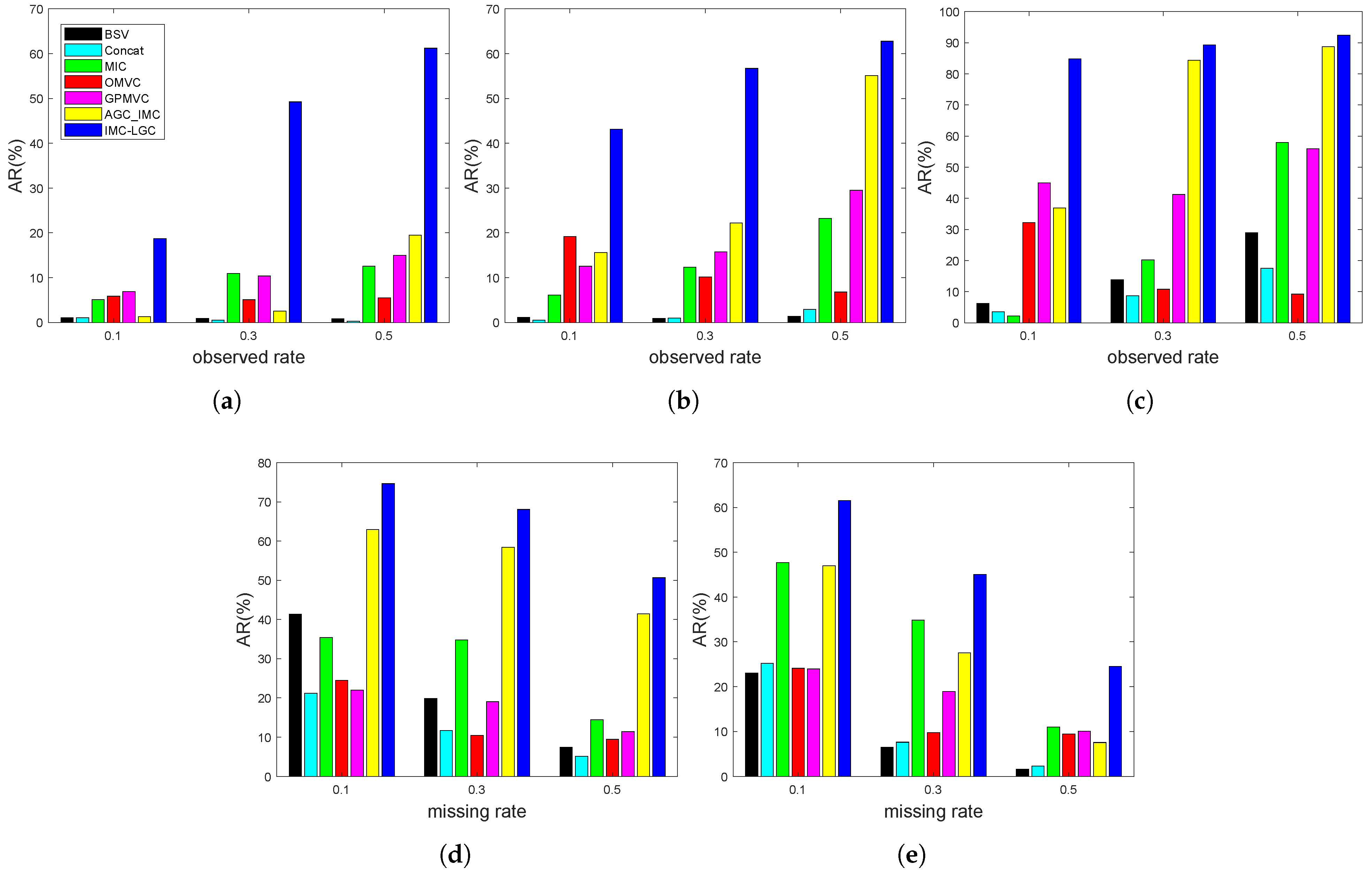
To evaluate the performance of the proposed method and its compared methods, Four well-known evaluation metrics, i.e., accuracy (ACC), normalized mutual information (NMI), purity, adjusted Rand index (AR), were adopted in our experiment [52,53,54], where ACC, NMI, and purity are reported in the table, and AR is shown in the figure. A higher value of these methods means a better clustering performance. For a fair comparison, we ran the above methods 10 times with respect to different view-missing groups, and then collected their average values (%). In addition, all compared methods were implemented with wide parameter ranges and their best performances were reported.

4.3. Experiment Results and Analysis

Experimental results of different incomplete multi-view clustering methods on the above two types of incomplete multi-view databases are enumerated in

Table 1. Average values of ACC (%), NMI (%), and purity (%) of different methods on the BBCSport dataset with different observed rates of paired samples. Bold numbers denote the best results.

	ACC			NMI			Purity
Method\Rate	0.1	0.3	0.5	0.1	0.3	0.5	0.1	0.3	0.5
BSV	34.05	33.71	33.53	12.19	11.76	11.50	34.57	34.40	34.40
Concat	32.84	32.50	32.41	12.68	11.24	9.68	34.22	33.97	34.05
MIC	40.34	46.64	47.07	19.54	28.10	29.04	44.74	50.17	49.83
OMVC	39.31	38.28	37.59	14.72	13.63	15.30	41.12	40.09	40.69
GPMVC	39.05	42.84	45.86	14.81	18.66	22.38	43.71	47.84	50.78
AGC_IMC	30.60	36.12	49.05	7.71	15.01	34.82	39.31	42.07	51.98
IMC-LGC	48.53	70.25	78.18	22.48	50.00	64.28	53.79	75.43	84.48

,

Table 2. Average values of ACC (%), NMI (%), and purity (%) of different methods in 3 source datasets with different observed rates of paired samples. Bold numbers denote the best results.

	ACC			NMI			Purity
Method\Rate	0.1	0.3	0.5	0.1	0.3	0.5	0.1	0.3	0.5
BSV	35.27	35.33	35.15	11.20	11.32	12.05	36.21	36.27	36.39
Concat	34.97	35.56	38.52	11.45	12.31	16.67	36.51	37.75	41.42
MIC	40.83	45.09	52.37	28.95	36.89	46.28	51.12	56.75	62.19
OMVC	45.74	40.89	38.11	35.13	27.93	22.76	58.28	51.89	47.99
GPMVC	38.76	42.01	52.07	20.88	26.24	34.33	50.36	54.44	61.48
AGC_IMC	35.15	45.98	72.84	31.85	39.69	61.94	59.76	62.49	78.05
IMC-LGC	59.82	79.64	79.34	49.79	64.65	65.74	71.24	80.29	81.24

,

Table 3. Average values of ACC (%), NMI (%), and purity (%) of different methods on the handwritten dataset with different observed rates of paired samples. Bold numbers denote the best results.

	ACC			NMI			Purity
Method\Rate	0.1	0.3	0.5	0.1	0.3	0.5	0.1	0.3	0.5
BSV	46.30	56.85	68.65	29.43	38.16	49.41	46.45	56.85	68.65
Concat	41.70	48.05	56.80	28.23	25.61	34.54	41.70	48.05	56.80
MIC	37.15	47.80	78.75	17.18	29.75	61.23	37.30	48.75	78.80
OMVC	57.45	42.15	40.05	41.74	19.15	16.86	58.95	42.50	40.55
GPMVC	71.85	67.05	78.75	51.43	46.80	58.81	71.85	68.25	78.80
AGC_IMC	58.35	93.80	95.60	55.51	83.04	87.15	62.20	93.80	95.60
IMC-LGC	93.95	95.85	97.10	83.35	87.72	90.96	93.95	95.85	97.10

,

Table 4. Average values of ACC (%), NMI (%), and purity (%) of different methods on the MSRC-v1 dataset with different missing view rates. Bold numbers denote the best results.

	ACC			NMI			Purity
Method\Rate	0.1	0.3	0.5	0.1	0.3	0.5	0.1	0.3	0.5
BSV	65.86	53.10	40.10	54.96	43.32	33.06	66.52	53.52	40.76
Concat	44.33	39.81	34.71	36.76	30.41	25.57	46.86	40.71	35.57
MIC	59.19	55.86	41.71	50.20	50.22	32.19	61.29	59.33	42.71
OMVC	48.81	35.62	35.57	37.31	25.22	24.74	50.05	36.62	37.14
GPMVC	46.86	42.48	35.67	34.42	31.60	22.66	48.81	43.33	37.19
AGC_IMC	75.10	74.33	66.10	75.20	69.29	56.23	78.43	76.90	66.76
IMC-LGC	87.80	87.80	77.61	78.91	77.67	62.89	87.80	87.80	77.66

and

Table 5. Average values of ACC (%), NMI (%), and purity (%) of different methods on the ORL dataset with different missing view rates. Bold numbers denote the best results.

	ACC			NMI			Purity
Method\Rate	0.1	0.3	0.5	0.1	0.3	0.5	0.1	0.3	0.5
BSV	48.85	37.25	26.40	69.10	56.54	44.92	54.18	40.98	30.05
Concat	49.15	38.63	28.90	68.76	57.59	47.73	53.43	42.25	32.03
MIC	61.10	54.45	30.58	79.13	73.29	52.94	65.25	59.23	33.58
OMVC	41.48	29.90	29.55	63.96	51.64	51.42	44.30	32.33	31.88
GPMVC	42.30	37.90	30.53	63.30	59.20	51.48	44.75	40.35	32.78
AGC_IMC	69.50	55.93	35.63	83.51	72.76	55.94	72.78	59.73	38.15
IMC-LGC	74.95	63.45	45.25	84.96	77.08	63.67	76.12	65.66	47.57

and Figure 2. These experimental results reflect the following points:

(1) The proposed method obtains significantly better results than the other methods in the five multi-view datasets under two types of incomplete cases. For example, as observed from Table 1, compared with the suboptimal method, the ACC value of the proposed method is improved by about 8%. As shown in Table 2, the ACC achieved by the proposed method is about 7% higher than that of the suboptimal method.

(2) As the observed rate of paired samples increase or the missing rate of view decreases, the BSV and Concat methods fail to obtain obvious improvements in comparison with other methods under our considered cases. For example, the BSV obtains results of 34.05%, 33.71%, and 33.53% of ACC in the BBCSport dataset with observed rates of 0.1, 0.3, and 0.5, respectively; the Concat achieves results of 32.84%, 32.50%, and 32.41% of ACC. These results indicate that the capabilities of BSV and Concat in capturing information are obviously weaker than other methods in dealing with incomplete multi-view data clustering problems, which are mainly caused by their rough processing.

(3) AGC_IMC is most related to our proposed method, IMC-LGC, while it fails to obtain competitive results in most cases, especially when the observed samples are smaller. For example, in Table 3, AGC_IMC obtains 93.80% and the proposed method achieves 95.85% in ACC under the observed rate of 0.3, while AGC_IMC only obtains 58.35% and the proposed method obtains 93.95% in ACC when the observed rate decreases to 0.1. In Table 4, when the missing rate of each view is 0.1, the ACC obtained by AGC_IMC is about 6% smaller than that of the proposed method, i.e., AGC_IMC obtains 69.50% and the proposed method obtains 74.95%; when the missing rate achieves 0.5, the ACC obtained by AGC_IMC is about 10% smaller than that of the proposed method, i.e., AGC_IMC obtains 35.63% and the proposed method obtains 45.25%. These results may be caused by the fact that AGC_IMC only learns the between-view inferring of missing instances and available instances, while the proposed method can capture the low-rank information (within and between views) simultaneously.

4.4. Sensitivity Analysis of the Penalty Parameters

The proposed method has three penalty parameters $\lambda , \gamma , \mathrm{and} \mu$, where $\lambda$ and $\gamma$ are the penalty parameters for low-rank constraint terms, and $\mu$ for the multi-view spectral clustering terms. Next, we analyze the sensitivities of these parameters in terms of clustering accuracy.

4.4.1. Parameters $\lambda$ and $\gamma$

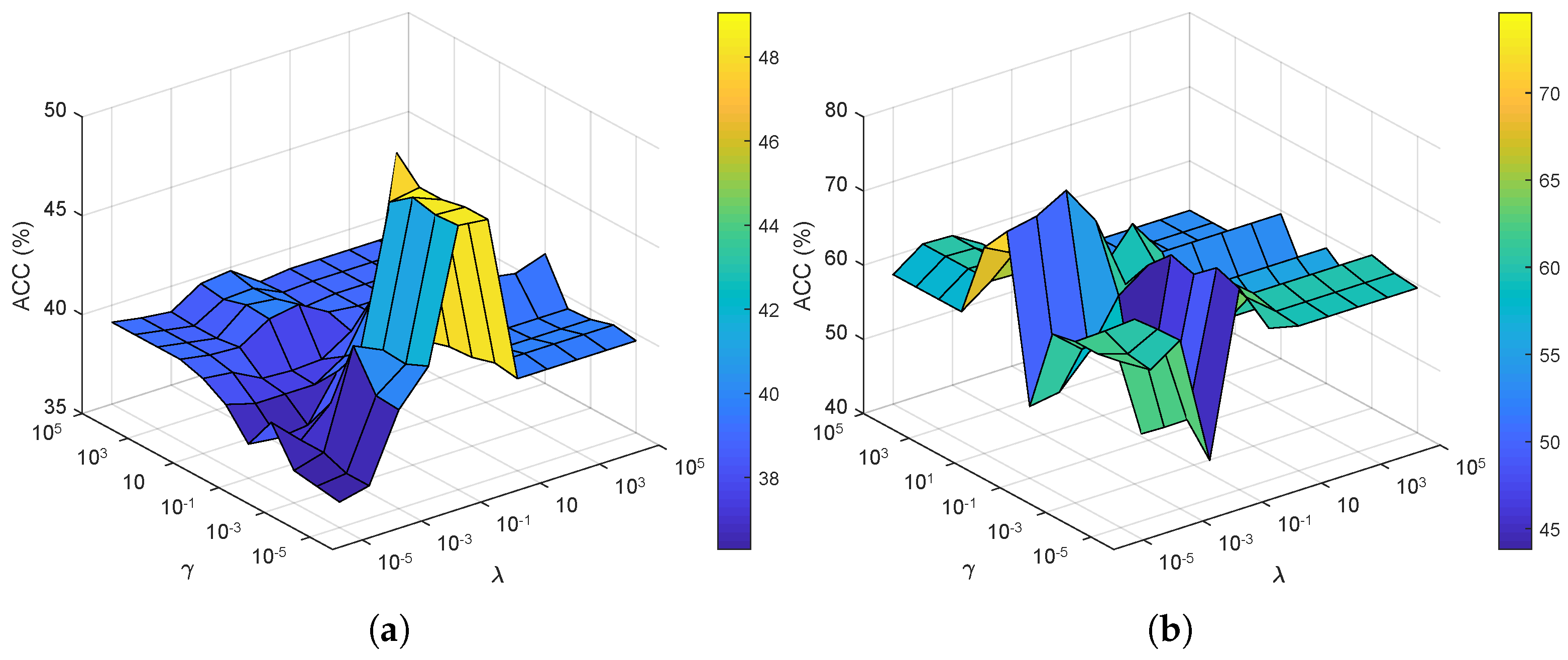
We experimented on the BBCSport dataset with 10% observed paired samples and the MSRC-v1 dataset with 50% missing instances of each view, under different combinations of parameters $\lambda$ and $\gamma$, where $\mu$ is fixed. In the experiment, $\lambda$ and $\gamma$ are selected from a set $\{{10}^{-5},{10}^{-4},{10}^{-3},{10}^{-2},{10}^{-1},1,{10}^1,{10}^2,{10}^3,{10}^4,{10}^5\}$ and $\mu$ is simply fixed by ${10}^{-3}$ for BBCSport and ${10}^{-1}$ for MSRC-v1. The experimental results of the proposed method on the above two datasets are recorded in Figure 3. As for the BBCSport dataset, a relatively good clustering performance could be achieved when $\lambda \in [{10}^{-1},1]$ and $\gamma \in [{10}^{-5},{10}^{-1}]$. As for the MSRC-v1 dataset, the proposed method can obtain the best results when $\lambda$ and $\gamma$ satisfy $\lambda \in [{10}^{-4},{10}^{-1}],\gamma \in [{10}^{-3},1]$. These results led us to choose parameters $\lambda$ and $\gamma$ of the proposed method in experiments with high clustering accuracy. According to the above-mentioned analysis, the parameters $\lambda$ and $\gamma$ are often selected from the set of $[{10}^{-4},{10}^{-1}]$ in our previous experiments.

4.4.2. Parameters $\mu$

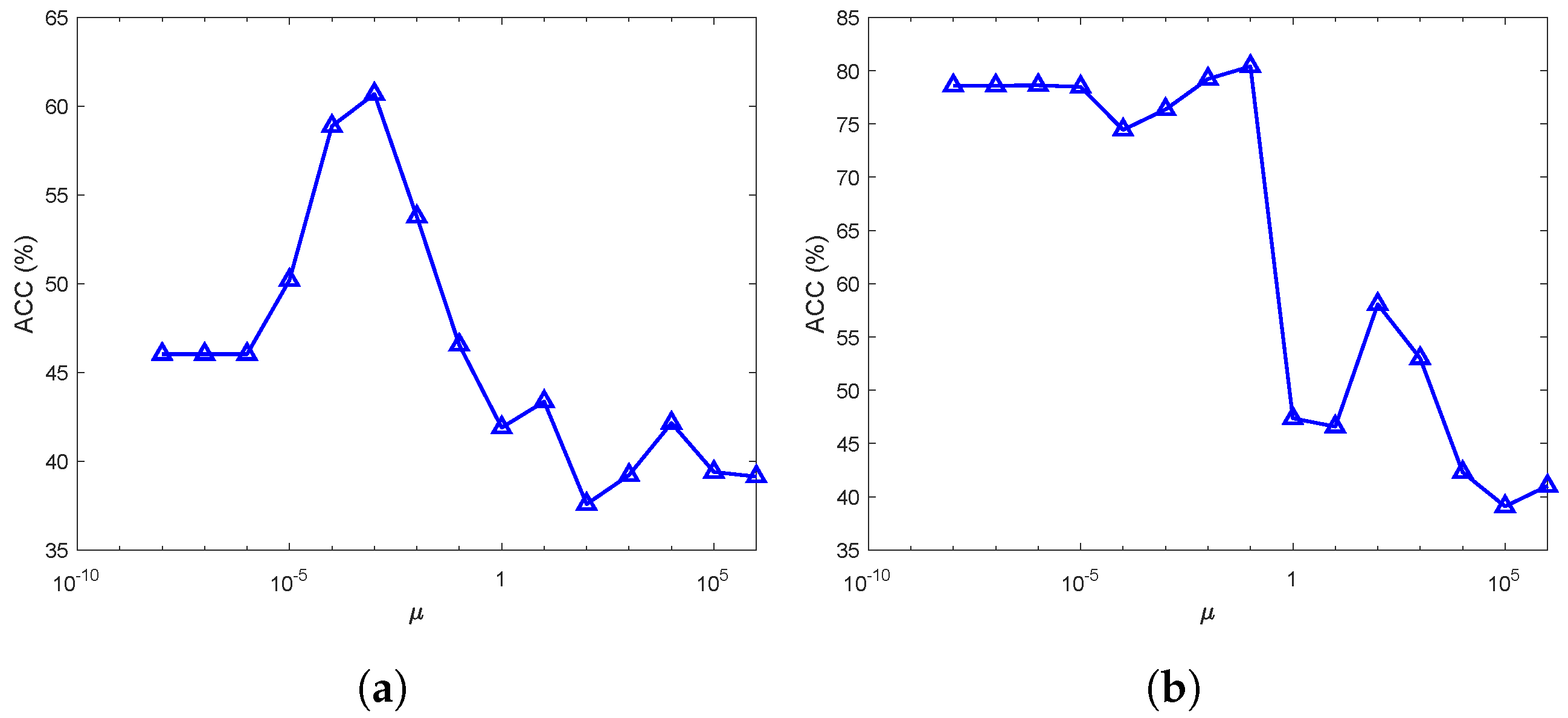
We conducted our experiment on the BBCSport dataset with 20% observed paired samples and the MSRC-v1 dataset with 30% missing instances of each view, under different values of parameter $\mu$, where $\lambda$ and $\gamma$ are fixed. In the experiment, $\mu$ is selected from a set $\{{10}^{-8},{10}^{-7},\cdots ,{10}^{-1},1,{10}^1,{10}^2,{10}^3,{10}^4,{10}^5,{10}^6\}$. As for these two datasets, $\lambda$ and $\gamma$ are simply fixed by ${10}^{-1}$ and ${10}^{-3}$, respectively. The experimental results of the proposed method are recorded in Figure 4, from which we can observe that the proposed method can obtain a rather good performance when $\mu$ is selected from $[{10}^{-5},{10}^{-1}]$. Specifically, the proposed method obtained the best results in the BBCSport dataset when $\mu ={10}^{-3}$, and in the MSRC-v1 dataset when $\mu ={10}^{-1}$. These results led us to choose parameter $\mu$ of the proposed method in experiments with high clustering accuracy. According to the above analysis, parameter $\mu$ was experimentally selected from the set of $[{10}^{-5},{10}^{-1}]$ in our previous experiments.

4.5. Convergence Analysis

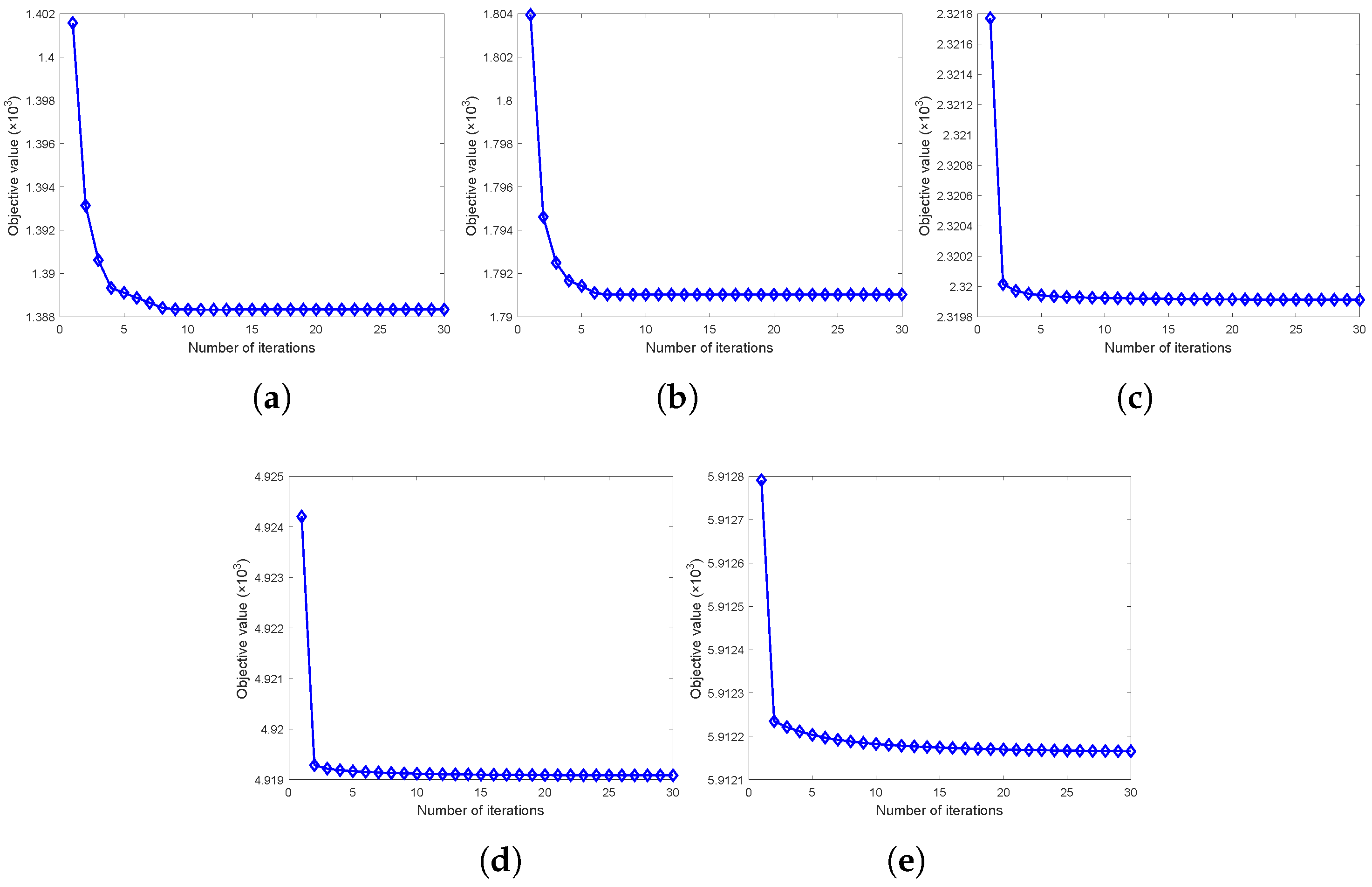
In this section, we experiment on the BBCSport dataset, the 3-sources dataset, the handwritten dataset with 30% observed paired samples, the MSRC-v1 dataset, and the ORL dataset with 30% missing view rates. We record the objective function value versus the iteration in Figure 5. From Figure 5, we can see that the objective function value fast decreased to the stationary point when the iteration increased, which reflects the relatively good convergence property of the proposed method.

5. Conclusions

This paper propose a novel method for the incomplete multi-view clustering problem via low-rank graph tensor completion, with the aim of exploiting the information hidden in missing views. Specifically, the proposed method stacks all similarity graphs into a third-order graph tensor and then exploits the low-rank relationship from each mode using the matrix nuclear norm. In this way, the connections hidden between the missing and available instances can be restored. The consensus representation was learned from all of the completed graphs via the multi-view spectral clustering. To obtain the optimal multi-view clustering results, the graph completion and consensus representation learning were developed to optimize jointly in a unified framework. Extensive experimental results conducted on several incomplete multi-view datasets show that the proposed method outperforms state-of-the-art incomplete multi-view clustering methods.

References

1. Mari nas-Collado, I.; Sipols, A.E.; Santos-Martín, M.T.; Frutos-Bernal, E. Clustering and Forecasting Urban Bus Passenger Demand with a Combination of Time Series Models. Mathematics 2022, 10, 2670. [Google Scholar] [CrossRef]
2. Lukauskas, M.; Ruzgas, T. A New Clustering Method Based on the Inversion Formula. Mathematics 2022, 10, 2559. [Google Scholar] [CrossRef]
3. Sarfraz, S.; Sharma, V.; Stiefelhagen, R. Efficient parameter-free clustering using first neighbor relations. In Proceedings of the IEEE/CVF Conference on Computer Vision and Pattern Recognition, Long Beach, CA, USA, 15–20 June 2019; pp. 8934–8943. [Google Scholar]
4. Wu, B.; Hu, B.G.; Ji, Q. A coupled hidden markov random field model for simultaneous face clustering and tracking in videos. Pattern Recognit. 2017, 64, 361–373. [Google Scholar] [CrossRef] [Green Version]
5. Bazzica, A.; Liem, C.C.; Hanjalic, A. Exploiting scene maps and spatial relationships in quasi-static scenes for video face clustering. Image Vis. Comput. 2017, 57, 25–43. [Google Scholar] [CrossRef]
6. Foggia, P.; Percannella, G.; Sansone, C.; Vento, M. Benchmarking graph-based clustering algorithms. Image Vis. Comput. 2009, 27, 979–988. [Google Scholar] [CrossRef]
7. Zhao, P.; Wu, H.; Huang, S. Multi-View Graph Clustering by Adaptive Manifold Learning. Mathematics 2022, 10, 1821. [Google Scholar] [CrossRef]
8. Prakoonwit, S.; Benjamin, R. 3D surface point and wireframe reconstruction from multiview photographic images. Image Vis. Comput. 2007, 25, 1509–1518. [Google Scholar] [CrossRef]
9. Yin, H.; Hu, W.; Zhang, Z.; Lou, J.; Miao, M. Incremental multi-view spectral clustering with sparse and connected graph learning. Neural Netw. 2021, 144, 260–270. [Google Scholar] [CrossRef]
10. Nie, F.; Li, J.; Li, X. Self-weighted Multiview Clustering with Multiple Graphs. In Proceedings of the IJCAI, Melbourne, Australia, 19–25 August 2017; pp. 2564–2570. [Google Scholar]
11. Zhao, N.; Bu, J. Robust multi-view subspace clustering based on consensus representation and orthogonal diversity. Neural Netw. 2022, 150, 102–111. [Google Scholar] [CrossRef]
12. Bickel, S.; Scheffer, T. Multi-view clustering. In Proceedings of the ICDM, Leipzig, Germany, 4–7 July 2004; Volume 4, pp. 19–26. [Google Scholar]
13. Cai, X.; Nie, F.; Huang, H. Multi-view k-means clustering on big data. In Proceedings of the Twenty-Third International Joint Conference on Artificial Intelligence, Beijing, China, 3–9 August 2013. [Google Scholar]
14. Chaudhuri, K.; Kakade, S.M.; Livescu, K.; Sridharan, K. Multi-view clustering via canonical correlation analysis. In Proceedings of the 26th Annual International Conference On machine Learning, Montreal, QC, Canada, 14–18 June 2009; pp. 129–136. [Google Scholar]
15. Kumar, A.; Rai, P.; Daume, H. Co-regularized multi-view spectral clustering. Adv. Neural Inf. Process. Syst. 2011, 24, 1413–1421. [Google Scholar]
16. Liu, J.; Wang, C.; Gao, J.; Han, J. Multi-view clustering via joint nonnegative matrix factorization. In Proceedings of the 2013 SIAM International Conference on Data Mining, SIAM, Austin, Texas, USA, 2–4 May 2013; pp. 252–260. [Google Scholar]
17. Kalayeh, M.M.; Idrees, H.; Shah, M. NMF-KNN: Image annotation using weighted multi-view non-negative matrix factorization. In Proceedings of the IEEE Conference on Computer Vision and Pattern Recognition, Columbus, OH, USA, 23–28 June 2014; pp. 184–191. [Google Scholar]
18. Zhao, H.; Ding, Z.; Fu, Y. Multi-view clustering via deep matrix factorization. In Proceedings of the Thirty-First AAAI Conference on Artificial Intelligence, San Francisco, CA, USA, 4–9 February 2017. [Google Scholar]
19. Huang, S.; Kang, Z.; Xu, Z. Auto-weighted multi-view clustering via deep matrix decomposition. Pattern Recognit. 2020, 97, 107015. [Google Scholar] [CrossRef]
20. Li, S.Y.; Jiang, Y.; Zhou, Z.H. Partial multi-view clustering. In Proceedings of the AAAI Conference on Artificial Intelligence, Québec City, QC, Canada, 27–31 July 2014; Volume 28. [Google Scholar]
21. Rai, N.; Negi, S.; Chaudhury, S.; Deshmukh, O. Partial multi-view clustering using graph regularized NMF. In Proceedings of the 2016 23rd International Conference on Pattern Recognition (ICPR), Cancun, Mexico, 4–8 December 2016; pp. 2192–2197. [Google Scholar]
22. Rai, P.; Trivedi, A.; Daumé III, H.; DuVall, S.L. Multiview clustering with incomplete views. In Proceedings of the NIPS Workshop on Machine Learning for Social Computing, Whilster, BC, Canada, 11 December 2010. [Google Scholar]
23. Wen, J.; Zhang, Z.; Zhang, Z.; Fei, L.; Wang, M. Generalized incomplete multiview clustering with flexible locality structure diffusion. IEEE Trans. Cybern. 2020, 51, 101–114. [Google Scholar] [CrossRef] [PubMed]
24. Zhao, H.; Liu, H.; Fu, Y. Incomplete multi-modal visual data grouping. In Proceedings of the IJCAI, New York, NY, USA, 9–15 July 2016; pp. 2392–2398. [Google Scholar]
25. Xu, N.; Guo, Y.; Zheng, X.; Wang, Q.; Luo, X. Partial multi-view subspace clustering. In Proceedings of the 26th ACM International Conference on Multimedia, Seoul, Republic of Korea, 22–26 October 2018; pp. 1794–1801. [Google Scholar]
26. Shao, W.; He, L.; Philip, S.Y. Multiple incomplete views clustering via weighted nonnegative matrix factorization with l2,1 regularization. In Proceedings of the Joint European Conference on Machine Learning and Knowledge Discovery in Databases, Porto, Portugal, 7–11 September 2015; Springer: Berlin/Heidelberg, Germany, 2015; pp. 318–334. [Google Scholar]
27. Shao, W.; He, L.; Lu, C.t.; Philip, S.Y. Online multi-view clustering with incomplete views. In Proceedings of the 2016 IEEE International Conference on Big Data (Big Data), Washington, DC, USA, 5–8 December 2016; pp. 1012–1017. [Google Scholar]
28. Hu, M.; Chen, S. Doubly aligned incomplete multi-view clustering. arXiv 2019, arXiv:1903.02785. [Google Scholar]
29. Wen, J.; Xu, Y.; Liu, H. Incomplete multiview spectral clustering with adaptive graph learning. IEEE Trans. Cybern. 2018, 50, 1418–1429. [Google Scholar] [CrossRef] [PubMed]
30. Wang, H.; Zong, L.; Liu, B.; Yang, Y.; Zhou, W. Spectral perturbation meets incomplete multi-view data. arXiv 2019, arXiv:1906.00098. [Google Scholar]
31. Wu, J.; Zhuge, W.; Tao, H.; Hou, C.; Zhang, Z. Incomplete multi-view clustering via structured graph learning. In Proceedings of the Pacific Rim International Conference on Artificial Intelligence, Nanjing, China, 28–31 August 2018; Springer: Berlin/Heidelberg, Germany, 2018; pp. 98–112. [Google Scholar]
32. Liu, X.; Zhu, X.; Li, M.; Wang, L.; Zhu, E.; Liu, T.; Kloft, M.; Shen, D.; Yin, J.; Gao, W. Multiple kernel k k-means with incomplete kernels. IEEE Trans. Pattern Anal. Mach. Intell. 2019, 42, 1191–1204. [Google Scholar] [CrossRef] [Green Version]
33. Wen, J.; Yan, K.; Zhang, Z.; Xu, Y.; Wang, J.; Fei, L.; Zhang, B. Adaptive graph completion based incomplete multi-view clustering. IEEE Trans. Multimed. 2020, 23, 2493–2504. [Google Scholar] [CrossRef]
34. Liu, G.; Lin, Z.; Yan, S.; Sun, J.; Yu, Y.; Ma, Y. Robust recovery of subspace structures by low-rank representation. IEEE Trans. Pattern Anal. Mach. Intell. 2012, 35, 171–184. [Google Scholar] [CrossRef] [Green Version]
35. Kolda, T.G.; Bader, B.W. Tensor Decompositions and Applications. SIAM Rev. 2009, 51, 455–500. [Google Scholar] [CrossRef]
36. Ng, A.Y.; Jordan, M.I.; Weiss, Y. On spectral clustering: Analysis and an algorithm. In Proceedings of the Advances in Neural Information Processing Systems, Vancouver, BC, Canada, 9–14 December 2002; pp. 849–856. [Google Scholar]
37. Hagen, L.; Kahng, A.B. New spectral methods for ratio cut partitioning and clustering. IEEE Trans. Comput.-Aided Des. Integr. Circuits Syst. 1992, 11, 1074–1085. [Google Scholar] [CrossRef] [Green Version]
38. Shi, J.; Malik, J. Normalized cuts and image segmentation. IEEE Trans. Pattern Anal. Mach. Intell. 2000, 22, 888–905. [Google Scholar]
39. Gao, H.; Nie, F.; Li, X.; Huang, H. Multi-view subspace clustering. In Proceedings of the IEEE International Conference on Computer Vision, Santiago, Chile, 7–13 December 2015; pp. 4238–4246. [Google Scholar]
40. Nie, F.; Wang, X.; Jordan, M.; Huang, H. The constrained laplacian rank algorithm for graph-based clustering. In Proceedings of the AAAI Conference on Artificial Intelligence, Phoenix, AZ, USA, 12–17 February 2016; Volume 30. [Google Scholar]
41. Ma, S.; Goldfarb, D.; Chen, L. Fixed point and Bregman iterative methods for matrix rank minimization. Math. Program. 2011, 128, 321–353. [Google Scholar] [CrossRef]
42. Cai, J.F.; Candès, E.J.; Shen, Z. A singular value thresholding algorithm for matrix completion. SIAM J. Optim. 2010, 20, 1956–1982. [Google Scholar] [CrossRef]
43. Naldi, M.C.; Campello, R.J.; Hruschka, E.R.; Carvalho, A. Efficiency issues of evolutionary k-means. Appl. Soft Comput. 2011, 11, 1938–1952. [Google Scholar] [CrossRef]
44. Mousa, A.; El-Shorbagy, M.; Farag, M. K-means-clustering based evolutionary algorithm for multi-objective resource allocation problems. Appl. Math. Inf. Sci 2017, 11, 1681–1692. [Google Scholar] [CrossRef]
45. Kwedlo, W. A clustering method combining differential evolution with the K-means algorithm. Pattern Recognit. Lett. 2011, 32, 1613–1621. [Google Scholar] [CrossRef]
46. Tabatabaei, S.S.; Coates, M.; Rabbat, M. GANC: Greedy agglomerative normalized cut for graph clustering. Pattern Recognit. 2012, 45, 831–843. [Google Scholar] [CrossRef]
47. Tabatabaei, S.S.; Coates, M.; Rabbat, M. Ganc: Greedy agglomerative normalized cut. arXiv 2011, arXiv:1105.0974. [Google Scholar]
48. Wright, T.G.; Trefethen, L.N. Large-scale computation of pseudospectra using ARPACK and eigs. SIAM J. Sci. Comput. 2001, 23, 591–605. [Google Scholar] [CrossRef]
49. Greene, D.; Cunningham, P. Practical solutions to the problem of diagonal dominance in kernel document clustering. In Proceedings of the 23rd International Conference on Machine Learning, Pittsburgh, PA, USA, 25–29 June 2006; pp. 377–384. [Google Scholar]
50. Winn, J.; Jojic, N. Locus: Learning object classes with unsupervised segmentation. In Proceedings of the Tenth IEEE International Conference on Computer Vision (ICCV’05) Volume 1, Washington, DC, USA, 17–20 October 2005; Volume 1, pp. 756–763. [Google Scholar]
51. Nie, F.; Cai, G.; Li, J.; Li, X. Auto-weighted multi-view learning for image clustering and semi-supervised classification. IEEE Trans. Image Process. 2017, 27, 1501–1511. [Google Scholar] [CrossRef]
52. Zhang, C.; Fu, H.; Liu, S.; Liu, G.; Cao, X. Low-rank tensor constrained multiview subspace clustering. In Proceedings of the IEEE International Conference on Computer Vision, Santiago, Chile, 7–13 December 2015; pp. 1582–1590. [Google Scholar]
53. Schütze, H.; Manning, C.D.; Raghavan, P. Introduction to Information Retrieval; Cambridge University Press: Cambridge, UK, 2008; Volume 39. [Google Scholar]
54. Hubert, L.; Arabie, P. Comparing partitions. J. Classif. 1985, 2, 193–218. [Google Scholar] [CrossRef]
Figure 1. Framework of the proposed incomplete multi-view clustering method, integrating the graph completion and consensus representation.
Mathematics 11 00652 g001
Figure 2. ARs (%) of different methods on the (a) BBCSport dataset, (b) 3 sources dataset, (c) Handwritten dataset with different observed rates of paired samples and on (d) MSRC-v1 dataset, (e) ORL dataset with different missing view rates.
Mathematics 11 00652 g002
Figure 3. ACC (%) versus parameters λ and γ of the proposed method on the (a) BBCSport dataset with 10% observed paired samples; (b) MSRC-v1 dataset with 50% missing instances of each view.
Mathematics 11 00652 g003
Figure 4. ACC (%) versus parameters μ of the proposed method on the (a) BBCSport dataset with 20% observed paired samples, (b) MSRC-v1 dataset with 30% missing instances of each view.
Mathematics 11 00652 g004
Figure 5. The convergence curves of the proposed method on five datasets: (a) BBCSport dataset, (b) 3-sources dataset, (c) handwritten dataset with 30% observed rates of paired samples, (d) MSRC-v1 dataset, and (e) ORL dataset with 30% missing view rates.
Mathematics 11 00652 g005