On Cauchy Problems of Caputo Fractional Differential Inclusion with an Application to Fractional Non-Smooth Systems

Abstract

In this innovative study, we investigate the properties of existence and uniqueness of solutions to initial value problem of Caputo fractional differential inclusion. In the study of existence problems, we considered the case of convex and non-convex multivalued maps. We obtained the existence results for both cases by means of the appropriate fixed point theorem. Furthermore, the uniqueness corresponding to both cases was also determined. Finally, we took a non-smooth system, the modified Murali–Lakshmanan–Chua (MLC) fractional-order circuit system, as an example to verify its existence and uniqueness conditions, and through several sets of simulation results, we discuss the implications.

1. Introduction

Because of the background of the applications of fractional calculus in applied mathematics, control systems, material mechanics, biophysics, biomedicine, viscoelasticity, and other areas, fractional calculus has received widespread attention. Fractional calculus and fractional differential equations have rapidly developed in both application and theory. For some specific applications of fractional calculus in various fields, see [1,2,3,4,5,6,7].

Fractional derivatives have global correlation properties and can accurately reflect the evolution of system functions that depend on their history. Therefore, they are commonly used to describe many physical phenomena in modeling [1,8,9,10]. However, because fractional derivatives have global and historical correlation properties, the numerical calculation of fractional differential equations is more difficult. Many electric and magnetic phenomena have been confirmed to be described by fractional calculus [11]. The results of the fractional order are more consistent with actual phenomena. This is mainly related to three types of electronic components: capacitors, inductors, and memristors.

The two most studied fractional derivatives are the Riemann–Liouville and Caputo fractional derivatives. Fractional differential equations has been extensively studied with respect to existence and uniqueness of their solutions [12,13,14,15]. In fractional differential equations, the initial value condition of the Riemann–Liouville type is of fractional order, while the initial value condition of the Caputo type is of integer order. The Caputo type has a more practical physical meaning, so it is often applied to various physical models. For a comparison of the properties of these two fractional derivatives and a theoretical analysis from an application point of view, see [16]. For a physical explanation of the two classes of fractional derivatives, please refer to [17].

Differential inclusion is a generalization of the concept of differential equations. In a dynamical system, it appears to provide the system with a set of possible forward directions at each moment, rather than a specific one. At present, it is widely used in game theory, control theory, optimization control, and other fields [18,19,20]. Differential inclusion theory is also a powerful tool for studying non-smooth dynamic systems [10,18,21,22]. Therefore, in order to study fractional non-smooth systems, we focus on fractional differential inclusion. Fractional-order non-smooth systems exhibit more complex dynamical behavior, and existing results and methods for integer-order non-smooth systems cannot be directly applied to them. Therefore, the problem is challenging.

Fractional differential inclusion is a relatively new area of research that began at the turn of the century. There are also some researches regarding the initial value problem and boundary value problem in fractional differential inclusion. The boundary value problem involving Caputo fractional differential inclusions has been extensively studied [23,24,25,26,27,28,29,30,31]. In recent years, some progress has been made in terms of the initial value problems of this type of differential equation. In 2019, Beddani and Hedia obtained the existence conditions of the solution set of the Riemann–Liouville fractional differential inclusion [32]. An existence result for differential inclusion involving the Caputo–Katugampola fractional derivative was also obtained [33]. In 2020, Gomoyunov investigated the Cauchy problem of Caputo fractional differential inclusion with an initial value condition extended to a finite interval [34]. In 2021, MikhailIn et al. studied a Cauchy problem for semi-linear Caputo fractional differential inclusion [35].

Herein, we study the solution set of Caputo fractional differential inclusion. We generalize the classical integer-order result in [36] to the Caputo fractional order. The conditions are improved compared to existing similar results. Equation (1) is the initial value problem (IVP) of differential inclusion that we will study.

$$\begin{array}{c}\hfill {}_0^C{D}_{\theta }^{\eta }\mu \in \mathcal{F}(\theta ,\mu \left(\theta \right))\mathrm{for}\mathrm{a}.\mathrm{e}.\theta \in \Delta =[0,T],\mu \left(0\right)={\mu }_0,0<\eta <1.\end{array}$$

(1)

$\mathcal{F}:\Delta \times {\mathbb{R}}^n\to \mathcal{P}\left({\mathbb{R}}^n\right)$ is a multivalued map, where $\mathcal{P}\left({\mathbb{R}}^n\right)$ is the family of all nonempty subsets of ${\mathbb{R}}^n$. What we are discussing is whether there exists a solution $\mu :\Delta \to {\mathbb{R}}^n$ such that $\mu \left(0\right)={\mu }_0$, ${}_0^C{D}_{\theta }^{\eta }\mu =h\left(\theta \right)\in \mathcal{F}(\theta ,\mu \left(\theta \right))$ a.e. on $\Delta$.

This paper comprises six sections. In Section 2, we introduce the definitions and properties of the fractional derivative and differential inclusion, as well as some lemmas that need to be used. For relevant definitions used in this paper, we refer to [1,36,37,38,39,40,41]. In Section 3, we consider the existence of solutions to IVP (1) when $\mathcal{F}:\Delta \times {\mathbb{R}}^n\to \mathcal{P}\left({\mathbb{R}}^n\right)$ is convex. This result is obtained from the fixed points of the set of compact Katutani maps in normed linear space. Further, we consider the existence of solutions to IVP (1) when $\mathcal{F}:\Delta \times {\mathbb{R}}^n\to \mathcal{P}\left({\mathbb{R}}^n\right)$ is non-convex. The result is given by the fixed point of the contraction multivalued map in the complete metric space. In Section 4, we consider the uniqueness of solutions of IVP (1). We obtain uniqueness results corresponding to both the convex and non-convex cases. In Section 5, we take the modified Murali–Lakshmanan–Chua (MLC) fractional-order circuit system as an example. We select four groups of different parameters for the system simulation to verify our theorems, and we conduct a brief discussion of the simulation results. In Section 6, we briefly summarize the work in this paper.

2. Preliminaries

In this section, we introduce the definitions and lemmas of fractional derivatives and differential inclusion, which are essential for this paper. For more on the definitions and properties of fractional derivatives, please refer to [1,39,40,41]. For more information and details about differential inclusion, see [36,37,38].

Definition 1

([42]). Let $\Delta =[0,T]$. ${\mathcal{L}}^1(\Delta ,{\mathbb{R}}^n)$ denotes the Banach space consisting of all Lebesgue integrable functions $h:\Delta \to {\mathbb{R}}^n$. The norm on this space is ${∥h∥}_{{\mathcal{L}}^1}={\int }_{\Delta }\left|h\right|d\theta$. $\mathcal{C}(\Delta ,{\mathbb{R}}^n)$ denotes the Banach space consisting of all continuous functions $h:\Delta \to {\mathbb{R}}^n$. The norm on this space is ${∥h∥}_{\infty }=sup\{\left|h\left(\theta \right)\right|:\theta \in \Delta \}$.

Definition 2

([40]). For the function $h\in {\mathcal{L}}^1(\Delta ,{\mathbb{R}}^n)$, its η-order fractional integral is as follows:

$${}_0{D}_{\theta }^{-\eta }h=\frac{1}{\Gamma \left(\eta \right)}{\int }_0^{\theta }{(\theta -\tau )}^{\eta -1}h\left(\tau \right){d}\tau ,$$

where $\eta >0$ and $\Gamma \left(·\right)$ is the Gamma function defined by

$$\Gamma \left(\eta \right)={\int }_0^{\infty }{\tau }^{\eta -1}{e}^{-\tau }{d}\tau .$$

Definition 3

([40]). For $h\in \mathcal{C}(\Delta ,{\mathbb{R}}^n)$, its η-order Caputo fractional derivative is as follows:

$${}_0^C{D}_{\theta }^{\eta }h=\frac{1}{\Gamma \left(n-\eta \right)}{\int }_0^{\theta }{(\theta -\tau )}^{-\eta +n-1}{h}^{\left(n\right)}\left(\tau \right){d}\tau ,$$

where $\eta >0$, $\eta \notin {\mathbb{N}}_{+}$, $n=\left[\eta \right]+1$.

Lemma 1

([1]). For $h\left(\theta \right)\in \mathcal{C}(\Delta ,{\mathbb{R}}^n)$, we first take its η-order fractional derivative and then take its η-order fractional integral. Then, we can obtain the following equation.

$${}_0{D}_{\theta }^{-\eta }{}_0^C{D}_{\theta }^{\eta }h=h\left(\theta \right)-h\left(0\right),$$

where $0<\eta <1$.

Lemma 2

([1]). For the function $h\left(\theta \right)\in {\mathcal{L}}^1(\Delta ,{\mathbb{R}}^n)$, we first take its η-order fractional integral and then take its η-order fractional derivative. Then, we can obtain the following equation.

$${}_0^C{D}_{\theta }^{\eta }{}_0{D}_{\theta }^{-\eta }h=h\left(\theta \right),$$

where $0<\eta <1$.

Definition 4

([40]). The Mittag–Leffler-type function in two parameters is given by

$$E_{i,j}\left(\theta \right)=\sum _{n=1}^{\infty }\frac{{\theta }^n}{\Gamma \left(in+j\right)},i>0,j>0.$$

When $j=1$, it is the Mittag–Leffler-type function in one parameter:

$$E_i\left(\theta \right)=\sum _{n=1}^{\infty }\frac{{\theta }^n}{\Gamma \left(in+1\right)}.$$

The Mittag–Leffler function is crucial for fractional differential equations. Its role is equivalent to that of the natural exponential function in integer-order differential equations.

Definition 5

([42]). We define ${\mathcal{P}}_{cl}\left(W\right)$, ${\mathcal{P}}_b\left(W\right)$, ${\mathcal{P}}_{cp}\left(W\right)$, and ${\mathcal{P}}_{cp,c}\left(W\right)$ in a metric space $(W,d)$ as follows:

$$\begin{array}{cc}\hfill & {\mathcal{P}}_{cl}\left(W\right)=\{Y\in \mathcal{P}\left(W\right):Y\mathit{is}\mathit{closed}\},\hfill \\ \hfill & {\mathcal{P}}_b\left(W\right)=\{Y\in \mathcal{P}\left(W\right):Y\mathit{is}\mathit{bounded}\},\hfill \\ \hfill & {\mathcal{P}}_{cp}\left(W\right)=\{Y\in \mathcal{P}\left(W\right):Y\mathit{is}\mathit{compact}\},\hfill \\ \hfill & {\mathcal{P}}_{cp,c}\left(W\right)=\{Y\in \mathcal{P}\left(W\right):Y\mathit{is}\mathit{compact}\mathit{and}\mathit{convex}\}.\hfill \end{array}$$

If for any $w\in {\mathbb{R}}^n$, the function $g\in {\mathcal{L}}^1(\Delta ,{\mathbb{R}}^n)$, then, $\mathcal{F}:\Delta \to {\mathcal{P}}_{cl}\left({\mathbb{R}}^n\right)$ is considered to be measurable, and g is defined as follows:

$$g\left(\theta \right)=d(w,\mathcal{F}(\theta \left)\right)=inf\left\{\right|w-h|:h\in \mathcal{F}(\theta \left)\right\}.$$

Definition 6

([36]). $\mathcal{F}:W\to \mathcal{P}\left(W\right)$ is said to be upper semi-continuous (u.s.c.) on W if it satisfies the following conditions (i) and (ii):

(i) 

For any $w\in W$, the set $\mathcal{F}\left(w\right)$ is a non-empty closed set and $\mathcal{F}\left(w\right)\subset W$;

(ii) 

For any $w\in W$ and open set $W_{*}$ such that $\mathcal{F}\left(w\right)\subseteq W_{*}\subseteq W$, there exists an open neighborhood $W_0$ of w such that $\mathcal{F}\left(W_0\right)={\bigcup }_{w\in W_0}\mathcal{F}\left(w\right)\subseteq W_{*}$.

For other equivalent definitions of upper semi-continuity, see [36].

Definition 7

([36]). $\mathcal{F}:\Delta \times W\to \mathcal{P}\left(W\right)$ is said to be a Carathéodory map if $\mathcal{F}$ satisfies the following conditions (i) and (ii):

(i) 

$\mathcal{F}(·,w)$ is measurable for each $w\in W$;

(ii) 

$\mathcal{F}(\theta ,·)$ is upper semi-continuous for almost all $\theta \in \Delta$.

Definition 8

([42]). Let $(W,d)$ be a metric space with $d(w_1,w_2)=\left|w_1-w_2\right|$, and the distance ${\mathcal{H}}_d:\mathcal{P}\left(W\right)\times \mathcal{P}\left(W\right)\to {\mathbb{R}}^{+}\bigcup \{\infty \}$ is defined as

$${\mathcal{H}}_d(W_1,W_2)=max\left\{\underset{w_1\in W_1}{sup}d(w_1,W_2),\underset{w_2\in W_2}{sup}d(W_1,w_2)\right\},$$

where $d(w_1,W_2)={inf}_{w_2\in W_2}d(w_1,w_2)$, $d(W_1,w_2)={inf}_{w_1\in W_1}d(w_1,w_2)$.

Definition 9

([42]). $\mathcal{N}:W\to {\mathcal{P}}_{cl}\left(W\right)$ is said to be a k-Lipschitz multivalued map if there exists $k\in {\mathbb{R}}^{+}$ such that

$${\mathcal{H}}_d(\mathcal{N}\left(w_1\right),\mathcal{N}\left(w_2\right))\le kd(w_1,w_2),\mathit{for}\mathit{any}{w}_1,w_2\in W.$$

If there exists $k<1$ that satisfies the above inequality, $\mathcal{N}$ is said to be a contraction multivalued map.

Lemma 3

([43]). Assuming that $(W,d)$ is a complete metric space. If $\mathcal{N}:W\to {\mathcal{P}}_{cl}\left(W\right)$ is a contraction multivalued map, then Fix$\mathcal{N}\ne \varnothing$, where Fix$\mathcal{N}$ is the set of fixed points of $\mathcal{N}$.

Lemma 4

([36]). Let $\mathcal{N}:W\to {\mathcal{P}}_{cl}\left(W\right)$ be a completely continuous operator. If $\mathcal{N}$ is a closed graph operator, then $\mathcal{N}$ is u.s.c. Further, if $\mathcal{N}$ is u.s.c., then $\mathcal{N}$ is a closed graph operator.

$\mathcal{N}$ is said to be a closed graph operator if, for $w_n\in W$, $\underset{n\to \infty }{lim}{w}_n=w$, ${\mu }_n\in \mathcal{N}\left(w_n\right)$, and $\underset{n\to \infty }{lim}{\mu }_n=\mu$, we have $\mu \in \mathcal{N}\left(w\right)$.

Definition 10

([44]). Let $W_1$ and $W_2$ be subsets of linear topological spaces. We assume that $W_2$ is convex. If $\mathcal{N}:W_1\to \mathcal{P}\left(W_2\right)$ is u.s.c. with non-empty compact convex values, then $\mathcal{N}$ is called a Kakutani map (or simply a $\mathbb{K}$-map).

Lemma 5

([44]). Let $W_1$ and $W_2$ be subsets of normed linear space. We assume that $W_1\subset W_2$ is open with $0\in W_1$ and $W_2$ is convex. Then, for $\mathcal{N}\in K_{\partial W_1}({\overline{W}}_1,\mathcal{P}\left(W_2\right))$, at least one of (a) and (b) is true.

(a) 

Fix$\mathcal{N}\ne \varnothing$;

(b) 

There exist $w\in \partial W_1$ and $\lambda \in (0,1)$ such that $w\in \lambda \mathcal{N}\left(w\right)$,

where $K_{\partial W_1}({\overline{W}}_1,\mathcal{P}\left(W_2\right))$ denotes the set of compact Kakutani maps $\mathcal{N}:{\overline{W}}_1\to \mathcal{P}\left(W_2\right)$ that are fixed-point-free on $\partial W_1$.

Lemma 6

([45]). Let $\left\{h_n\right\}$ be a sequence of a normed space W, where $n\in {\mathbb{N}}_{+}$. We assume that $\left\{h_n\right\}$ weakly converges to h in W. Then, there will be a sequence of convex combinations $\{{\mu }_m={\displaystyle \sum _{n=1}^m}{a}_{mn}{h}_n\}$ that strongly converges to h, where ${\displaystyle \sum _{n=1}^m}{a}_{mn}=1$ for $m\in {\mathbb{N}}_{+}$ and $a_{mn}\ge 0$ for $n=1,2,\dots ,m$.

Lemma 7

([38]). Let Y be a compact subset of a separable Banach space W and let $\left\{Y_n\right\}\subset Y$ be a sequence of subsets, where $n\in {\mathbb{N}}_{+}$. Then,

$$\overline{co}\left(\underset{n\to \infty }{lim}sup{Y}_n\right)=\bigcap _{m>0}\overline{co}\left(\bigcup _{n\ge m}{Y}_m\right),$$

where $\overline{co}\left(·\right)$ represents the closure of the convex hull of $\left(·\right)$.

Lemma 8

([38]). We assume that $W_1$, $W_2$ are two metric spaces. If $\mathcal{F}:W_1\to {\mathcal{P}}_{cp}\left(W_2\right)$ is u.s.c, then for each $w\in W_1$,

$$\underset{w^{*}\to w}{lim}sup\mathcal{F}\left(w^{*}\right)=\mathcal{F}\left(w\right).$$

Lemma 9

([46]). Let $\gamma \left(\theta \right)\in {\mathcal{L}}^1(\Delta ,{\mathbb{R}}^{+})$, $\zeta \left(\theta \right)\in \mathcal{C}(\Delta ,{\mathbb{R}}^{+})$, $\mu \left(\theta \right)\in {\mathcal{L}}^1(\Delta ,{\mathbb{R}}^{+})$, and $\zeta \left(\theta \right)$ be non-decreasing. There exists $\mathrm{M}>0$ such that $\gamma \left(\theta \right)$, $\zeta \left(\theta \right)\le \mathrm{M}$. If the following inequality holds:

$$\mu \left(\theta \right)\le \gamma \left(\theta \right)+\zeta \left(\theta \right){\int }_0^{\theta }{(\theta -\tau )}^{\eta -1}\mu \left(\tau \right){d}\tau ,$$

then

$$\mu \left(\theta \right)\le \gamma \left(\theta \right)+{\int }_0^{\theta }\sum _{m=1}^{\infty }\frac{{\left(\zeta \right(\theta )\Gamma (\eta \left)\right)}^m}{\Gamma \left(m\eta \right)}{(\theta -\tau )}^{m\eta -1}\gamma \left(\tau \right){d}\tau ,$$

where $\eta >0$, $\theta \in \Delta =[0,T]$.

3. Proof of the Existence of Solutions

We will first explain the equivalent form of IVP (1). Then, we will consider the existence result of IVP (1) when $\mathcal{F}:\Delta \times {\mathbb{R}}^n\to \mathcal{P}\left({\mathbb{R}}^n\right)$ is convex. The nonlinear Leray–Schauder-type alternative for compact Kakutani maps is the foundation for the proof of the result. A generalized Gronwall inequality is crucial in demonstrating that (b) of Lemma 5 does not hold.

Definition 11.

A function $\mu \left(\theta \right)\in \mathcal{C}(\Delta ,{\mathbb{R}}^n)$ is said to be a solution to IVP (1) if there exists an $h\left(\theta \right)\in {\mathcal{L}}^1(\Delta ,{\mathbb{R}}^n)$ such that ${}_0^C{D}_{\theta }^{\eta }\mu =h\left(\theta \right)$ on Δ for $h\left(\theta \right)\in \mathcal{F}(\theta ,\mu (\theta \left)\right)$ a.e. on Δ and $\mu \left(0\right)={\mu }_0$.

Lemma 10.

If $h\left(\theta \right)\in \mathcal{C}(\Delta ,{\mathbb{R}}^n)$, then the existence of solutions of IVP (2) is equivalent to the existence of solutions of integral Equation (3).

$$\begin{array}{c}\hfill \left\{\begin{array}{c}{}_0^C{D}_{\theta }^{\eta }\mu =h\left(\theta \right)\hfill \\ \mu \left(0\right)={\mu }_0\hfill \end{array}\right.\end{array}$$

(2)

where $0<\eta <1$, $\theta \in \Delta =[0,T]$.

$$\begin{array}{c}\hfill \mu \left(\theta \right)={\mu }_0+\frac{1}{\Gamma \left(\eta \right)}{\int }_0^{\theta }{(\theta -\tau )}^{\eta -1}h\left(\tau \right){d}\tau .\end{array}$$

(3)

Proof. 

Assuming that $\mu \left(\theta \right)$ satisfies (2), and taking the $\eta$-order integral on both sides of Equation ${}_0^C{D}_{\theta }^{\eta }\mu =h\left(\theta \right)$, then by Lemma 1, we have

$$\mu \left(\theta \right)-{\mu }_0=\frac{1}{\Gamma \left(\eta \right)}{\int }_0^{\theta }{(\theta -\tau )}^{\eta -1}h\left(\tau \right)\mathrm{d}\tau .$$

Therefore, $\mu \left(\theta \right)$ is also the solution of (3). Conversely, we assume that $\mu \left(\theta \right)$ satisfies (3), and we take the $\eta$-order derivative of Equation (3). From Lemma 2, we can obtain

$${}_0^C{D}_{\theta }^{\eta }\mu =h\left(\theta \right).$$

Therefore, the lemma holds. □

Definition 12.

For each $\mu \in \mathcal{C}(\Delta ,{\mathbb{R}}^n)$, the set of selections of $\mathcal{F}:\Delta \times {\mathbb{R}}^n\to \mathcal{P}\left({\mathbb{R}}^n\right)$ is given by

$$S_{\mathcal{F},\mu }=\{h\in {\mathcal{L}}^1(\Delta ,{\mathbb{R}}^n):h\left(\theta \right)\in \mathcal{F}(\theta ,\mu \left(\theta \right))\mathrm{a}.\mathrm{e}.\theta \in \Delta \}.$$

The following conditions will help us obtain the first existence result.

(D1)

$\mathcal{F}:\Delta \times {\mathbb{R}}^n\to {\mathcal{P}}_{cp,c}\left({\mathbb{R}}^n\right)$ is a Carathéodory map;

(D2)

There exist a bounded $\varphi \in {\mathcal{L}}^1(\Delta ,{\mathbb{R}}^{+})$ and a bounded $\rho \in {\mathcal{L}}^1(\Delta ,{\mathbb{R}}^{+})$ such that

$${\parallel \mathcal{F}(\theta ,w)\parallel }_{\mathcal{P}}=sup\left\{\right|h|:h\in \mathcal{F}(\theta ,w)\}\le \rho \left(\theta \right)\left|w\right|+\varphi \left(\theta \right)\mathrm{for}\theta \in \Delta \mathrm{and}\mathrm{each}w\in {\mathbb{R}}^n.$$

Theorem 1.

In IVP (1), we assume that $\mathcal{F}$ satisfies the conditions (D1) and (D2). Then, there is at least one solution to IVP (1).

Proof. 

We define a multivalued operator $\mathcal{N}:\mathcal{C}(\Delta ,{\mathbb{R}}^n)\to \mathcal{P}\left(\mathcal{C}(\Delta ,{\mathbb{R}}^n)\right)$ as

$$\mathcal{N}\left(\mu \right)=\{g\in \mathcal{C}(\Delta ,{\mathbb{R}}^n):g\left(\theta \right)={\mu }_0+\frac{1}{\Gamma \left(\eta \right)}{\int }_0^{\theta }{(\theta -\tau )}^{\eta -1}h\left(\tau \right){d}\tau ,h\in S_{\mathcal{F},\mu }\}.$$

If there exists a $\mu \in \mathrm{Fix}\mathcal{N}$, obviously, it also satisfies IVP (1). By the Leray–Schauder principle for compact Kakutani maps, it is proved that the operator $\mathcal{N}$ has a fixed point.

Step 1: For $\forall \mu \in \mathcal{C}(\Delta ,{\mathbb{R}}^n)$, the operator $\mathcal{N}\left(\mu \right)$ is convex.

Suppose that there exist $g_1$, $g_2\in \mathcal{N}\left(\mu \right)$, i.e., there exist $h_1$, $h_2\in S_{\mathcal{F},\mu }$ such that for each $\theta \in \Delta$,

$$g_m\left(\theta \right)={\mu }_0+\frac{1}{\Gamma \left(\eta \right)}{\int }_0^{\theta }{(\theta -\tau )}^{\eta -1}{h}_m\left(\tau \right){d}\tau ,m=1,2.$$

For each $0\le \lambda \le 1$,

$$[\lambda g_1+(1-\lambda )g_2]\left(\theta \right)={\mu }_0+\frac{1}{\Gamma \left(\eta \right)}{\int }_0^{\theta }{(\theta -\tau )}^{\eta -1}\left[\lambda h_1\left(\tau \right)+(\lambda -1)h_2\left(\tau \right)\right]{d}\tau .$$

Since $\mathcal{F}$ has convex values, $S_{\mathcal{F},\mu }$ is convex, so we have

$$\lambda g_1+(1-\lambda )g_2\in \mathcal{N}\left(\mu \right).$$

Step 2: $\mathcal{N}$ maps bounded sets into bounded sets in $\mathcal{C}(\Delta ,{\mathbb{R}}^n)$.

Let $B_r=\{\mu \in \mathcal{C}(\Delta ,{\mathbb{R}}^n):{∥\mu ∥}_{\infty }\le r\}$ be a bounded set in $\mathcal{C}(\Delta ,{\mathbb{R}}^n)$, where $r>0$. Then, for each $\mu \in B_r$, $g\in \mathcal{N}\left(\mu \right)$, we have

$$\begin{array}{cc}\hfill \left|g\left(\theta \right)\right|& \le \left|{\mu }_0\right|+\frac{1}{\Gamma \left(\eta \right)}{\int }_0^{\theta }{(\theta -\tau )}^{\eta -1}\left|h\left(\tau \right)\right|{d}\tau \hfill \\ \hfill & \le \left|{\mu }_0\right|+\frac{1}{\Gamma \left(\eta \right)}{\int }_0^{\theta }{(\theta -\tau )}^{\eta -1}[\rho \left(\tau \right)\left|\mu \left(\tau \right)\right|+\varphi \left(\tau \right)]\mathrm{d}\tau \hfill \\ \hfill & \le \left|{\mu }_0\right|+\frac{1}{\Gamma \left(\eta \right)}{\int }_0^{\theta }{(\theta -\tau )}^{\eta -1}[\rho \left(\tau \right){∥\mu ∥}_{\infty }+\varphi \left(\tau \right)]\mathrm{d}\tau \hfill \\ \hfill & \le \left|{\mu }_0\right|+\frac{r{∥\rho ∥}_{\infty }}{\Gamma \left(\eta \right)}{\int }_0^{\theta }{(\theta -\tau )}^{\eta -1}\mathrm{d}\tau +\frac{{∥\varphi ∥}_{\infty }}{\Gamma \left(\eta \right)}{\int }_0^{\theta }{(\theta -\tau )}^{\eta -1}\mathrm{d}\tau \hfill \\ \hfill & \le \left|{\mu }_0\right|+\frac{{\theta }^{\eta }[r{∥\rho ∥}_{\infty }+{∥\varphi ∥}_{\infty }]}{\Gamma \left(\eta +1\right)}\hfill \\ \hfill & \le \left|{\mu }_0\right|+\frac{T^{\eta }[r{∥\rho ∥}_{\infty }+{∥\varphi ∥}_{\infty }]}{\Gamma \left(\eta +1\right)}\hfill \end{array}$$

Thus, ${∥g∥}_{\infty }\le \left|{\mu }_0\right|+\frac{T^{\eta }[r{∥\rho ∥}_{\infty }+{∥\varphi ∥}_{\infty }]}{\Gamma \left(\eta +1\right)}<\infty$.

Step 3: $\mathcal{N}\left(B_r\right)$ is an equicontinuous set.

Let ${\theta }_1$, ${\theta }_2\in \Delta$, ${\theta }_1<{\theta }_2$, $B_r$ be a bounded set of $\mathcal{C}(\Delta ,{\mathbb{R}}^n)$, as in Step 2. Then, for each $\mu \in B_r$, $g\in \mathcal{N}\left(\mu \right)$, we have

$$\begin{array}{cc}\hfill & \left|g\left({\theta }_2\right)-g\left({\theta }_1\right)\right|\hfill \\ \hfill =& \left|\frac{1}{\Gamma \left(\eta \right)}{\int }_0^{{\theta }_2}{({\theta }_2-\tau )}^{\eta -1}h\left(\tau \right)\mathrm{d}\tau -\frac{1}{\Gamma \left(\eta \right)}{\int }_0^{{\theta }_1}{({\theta }_1-\tau )}^{\eta -1}h\left(\tau \right)\mathrm{d}\tau \right|\hfill \\ \hfill \le & \frac{1}{\Gamma \left(\eta \right)}{\int }_{{\theta }_1}^{{\theta }_2}{({\theta }_2-\tau )}^{\eta -1}\left|h\left(\tau \right)\right|\mathrm{d}\tau +\frac{1}{\Gamma \left(\eta \right)}{\int }_0^{{\theta }_1}\left|{({\theta }_2-\tau )}^{\eta -1}-{({\theta }_1-\tau )}^{\eta -1}\right|\left|h\left(\tau \right)\right|\mathrm{d}\tau \hfill \\ \hfill \le & \frac{r{∥\rho ∥}_{\infty }+{∥\varphi ∥}_{\infty }}{\Gamma \left(\eta +1\right)}{({\theta }_2-{\theta }_1)}^{\eta }+\frac{1}{\Gamma \left(\eta \right)}{\int }_0^{{\theta }_1}\left[{({\theta }_1-\tau )}^{\eta -1}-{({\theta }_2-\tau )}^{\eta -1}\right]\left|h\left(\tau \right)\right|\mathrm{d}\tau \hfill \\ \hfill \le & \frac{r{∥\rho ∥}_{\infty }+{∥\varphi ∥}_{\infty }}{\Gamma \left(\eta +1\right)}{({\theta }_2-{\theta }_1)}^{\eta }+\frac{r{∥\rho ∥}_{\infty }+{∥\varphi ∥}_{\infty }}{\Gamma \left(\eta +1\right)}\left[{({\theta }_2-{\theta }_1)}^{\eta }+{{\theta }_1}^{\eta }-{{\theta }_2}^{\eta }\right]\hfill \\ \hfill \le & \frac{r{∥\rho ∥}_{\infty }+{∥\varphi ∥}_{\infty }}{\Gamma \left(\eta +1\right)}\left[2{({\theta }_2-{\theta }_1)}^{\eta }+{{\theta }_1}^{\eta }-{{\theta }_2}^{\eta }\right]\hfill \end{array}$$

As ${\theta }_1\to {\theta }_2$, $(2{({\theta }_2-{\theta }_1)}^{\eta }+{{\theta }_1}^{\eta }-{{\theta }_2}^{\eta })\to 0$, thus, the proof of Step 3 is complete. Combining the proofs of Steps 2 and 3, we show that $\mathcal{N}$ satisfies the Arzelá–Ascoli theorem. It is proved that the map $\mathcal{N}:\mathcal{C}(\Delta ,{\mathbb{R}}^n)\to \mathcal{P}\left(\mathcal{C}(\Delta ,{\mathbb{R}}^n)\right)$ is a completely continuous operator.

Step 4: $\mathcal{N}$ is u.s.c.

We assume that ${\mu }_n\to {\mu }_{*}$, $g_n\in \mathcal{N}\left({\mu }_n\right)$, and $g_n\to g_{*}$. For the result that $\mathcal{N}$ is a closed graph, we need to prove that $g_{*}\in \mathcal{N}\left({\mu }_{*}\right)$. Since $g_n\in \mathcal{N}\left({\mu }_n\right)$, there exists $h_n\in S_{\mathcal{F},{\mu }_n}$ such that, for each $\theta \in \Delta$,

$$g_n\left(\theta \right)={\mu }_0+\frac{1}{\Gamma \left(\eta \right)}{\int }_0^{\theta }{(\theta -\tau )}^{\eta -1}{h}_n\left(\tau \right)\mathrm{d}\tau .$$

Since $\mathcal{F}:\Delta \times {\mathbb{R}}^n\to {\mathcal{P}}_{cp,c}\left({\mathbb{R}}^n\right)$ is u.s.c., then, for $\forall \epsilon >0$, there exists $n_0>0$ (the value of $n_0$ is related to $\epsilon$) such that, for $n>n_0$,

$$h_n\left(\theta \right)\in \mathcal{F}(\theta ,{\mu }_n\left(\theta \right))\subset \mathcal{F}(\theta ,{\mu }_{*}\left(\theta \right))+\epsilon B(0,1),\mathrm{a}.\mathrm{e}.\theta \in \Delta .$$

Since $\mathcal{F}(\theta ,w)$ is compact, then there exists a sub-sequence $\left\{h_{n_m}\right\}$ such that

$$h_{n_m}\to h_{*}\mathrm{as}m\to \infty .$$

For a.e. $\theta \in \Delta$, we define $h_{*}$ as follows:

$$g_{*}\left(\theta \right)={\mu }_0+\frac{1}{\Gamma \left(\eta \right)}{\int }_0^{\theta }{(\theta -\tau )}^{\eta -1}{h}_{*}\left(\tau \right)\mathrm{d}\tau .$$

We can still use the sequence $\left\{h_n\right\}$ to represent the sub-sequence $\left\{h_{n_m}\right\}$. Next, we prove that $h_{*}\left(\theta \right)\in \mathcal{F}(\theta ,{\mu }_{*}\left(\theta \right))$, a.e. $\theta \in \Delta$. From Lemma 6, there exists a sequence of convex combinations $f_m={\displaystyle \sum _{n=1}^m}{a}_{mn}{h}_n$ that strongly converges to $h_{*}$, where ${\displaystyle \sum _{n=1}^m}{a}_{mn}=1$ for $m\in {\mathbb{N}}_{+}$ and $a_{mn}\ge 0$ for $n=1,2,\dots ,m$. Then, from Lemma 7, we have

$$\begin{array}{cc}\hfill h_{*}\left(\theta \right)& \in \bigcap _{m\ge 1}\overline{\left\{f_m\left(\theta \right)\right\}}\mathrm{a}.\mathrm{e}.\theta \in \Delta \hfill \\ \hfill & \subset \bigcap _{m\ge 1}\overline{co}\{h_s\left(\theta \right),s\ge m\}\hfill \\ \hfill & \subset \bigcap _{m\ge 1}\overline{co}\left\{\bigcup _{s\ge m}\mathcal{F}(\theta ,{\mu }_s\left(\theta \right))\right\}\hfill \\ \hfill & =\overline{co}\{\underset{s\to \infty }{lim}sup\mathcal{F}(\theta ,{\mu }_s\left(\theta \right))\}.\hfill \end{array}$$

Since $\mathcal{F}:\Delta \times {\mathbb{R}}^n\to {\mathcal{P}}_{cp,c}\left({\mathbb{R}}^n\right)$ is u.s.c, then, by Lemma 8, we have

$$\underset{s\to \infty }{lim}sup\mathcal{F}(\theta ,{\mu }_s\left(\theta \right))=\mathcal{F}(\theta ,{\mu }_{*}\left(\theta \right)),\mathrm{a}.\mathrm{e}.\theta \in \Delta .$$

Therefore, $h_{*}\left(\theta \right)\in \overline{co}\left\{\mathcal{F}(\theta ,{\mu }_{*}\left(\theta \right))\right\}$, and $\mathcal{F}(\theta ,{\mu }_{*}\left(\theta \right))$ has convex and closed values, so we have $h_{*}\left(\theta \right)\in \mathcal{F}(\theta ,{\mu }_{*}\left(\theta \right))$. Thus, $g_{*}\in \mathcal{N}\left({\mu }_{*}\right)$, $\mathcal{N}$ has a closed graph. Then, by Lemma 4, $\mathcal{N}$ is u.s.c.

Step 5: A priori bounds on solutions.

Let $\mu \in \mathcal{C}(\Delta ,{\mathbb{R}}^n)$ be such that $\mu \in \lambda \mathcal{N}\left(\mu \right)$ for $\lambda \in (0,1)$. Then, there exists $h\in S_{\mathcal{F},\mu }$ such that, for each $\theta \in \Delta$,

$$\begin{array}{cc}\hfill \left|\mu \left(\theta \right)\right|& \le \left|{\mu }_0\right|+\frac{1}{\Gamma \left(\eta \right)}{\int }_0^{\theta }{(\theta -\tau )}^{\eta -1}\left|h\left(\tau \right)\right|\mathrm{d}\tau \hfill \\ \hfill & \le \left|{\mu }_0\right|+\frac{1}{\Gamma \left(\eta \right)}{\int }_0^{\theta }{(\theta -\tau )}^{\eta -1}[\rho \left(\tau \right)\left|\mu \left(\tau \right)\right|+\varphi \left(\tau \right)]\mathrm{d}\tau \hfill \\ \hfill & \le \left|{\mu }_0\right|+\frac{{∥\rho ∥}_{\infty }}{\Gamma \left(\eta \right)}{\int }_0^{\theta }{(\theta -\tau )}^{\eta -1}\left|\mu \left(\tau \right)\right|\mathrm{d}\tau +\frac{{∥\varphi ∥}_{\infty }}{\Gamma \left(\eta \right)}{\int }_0^{\theta }{(\theta -\tau )}^{\eta -1}\mathrm{d}\tau \hfill \\ \hfill & \le \left|{\mu }_0\right|+\frac{{\theta }^{\eta }{∥\varphi ∥}_{\infty }}{\Gamma \left(\eta +1\right)}+\frac{{∥\rho ∥}_{\infty }}{\Gamma \left(\eta \right)}{\int }_0^{\theta }{(\theta -\tau )}^{\eta -1}\left|\mu \left(\tau \right)\right|\mathrm{d}\tau \hfill \end{array}$$

We define $\gamma \left(\theta \right)=\left|{\mu }_0\right|+\frac{{\theta }^{\eta }{∥\varphi ∥}_{\infty }}{\Gamma \left(\eta +1\right)}$, $\zeta \left(\theta \right)=\frac{{∥\rho ∥}_{\infty }}{\Gamma \left(\eta \right)}$.

Since $\varphi \in {\mathcal{L}}^1(\Delta ,{\mathbb{R}}^{+})$ is bounded and $\rho \in {\mathcal{L}}^1(\Delta ,{\mathbb{R}}^{+})$ is bounded, we have that $\gamma \left(\theta \right)\in {\mathcal{L}}^1(\Delta ,{\mathbb{R}}^{+})$ and $\zeta \left(\theta \right)\in \mathcal{C}(\Delta ,{\mathbb{R}}^{+})$ are non-decreasing. Then, by Lemma 9,

$$\begin{array}{cc}\hfill \left|\mu \left(\theta \right)\right|& \le \gamma \left(\theta \right)+{\int }_0^{\theta }\sum _{m=1}^{\infty }\frac{{\left(\zeta \right(\theta )\Gamma (\eta \left)\right)}^m}{\Gamma \left(m\eta \right)}{(\theta -\tau )}^{m\eta -1}\gamma \left(\tau \right)\mathrm{d}\tau \hfill \\ \hfill & \le \gamma \left(\theta \right)+\gamma \left(\theta \right){\int }_0^{\theta }\sum _{m=1}^{\infty }\frac{{\left(\zeta \right(\theta )\Gamma (\eta \left)\right)}^m}{\Gamma \left(m\eta \right)}{(\theta -\tau )}^{m\eta -1}\mathrm{d}\tau \hfill \\ \hfill & \le \gamma \left(\theta \right)+\gamma \left(\theta \right)\sum _{m=1}^{\infty }\frac{{\left(\zeta \right(T)\Gamma (\eta \left)\right)}^m}{\Gamma \left(m\eta \right)}{\int }_0^{\theta }{(\theta -\tau )}^{m\eta -1}\mathrm{d}\tau \hfill \\ \hfill & \le \gamma \left(\theta \right)+\gamma \left(\theta \right)\sum _{m=1}^{\infty }\frac{{\left(\zeta \right(T)\Gamma (\eta \left)\right)}^m{\theta }^{m\eta }}{\Gamma (m\eta +1)}\hfill \\ \hfill & \le \gamma \left(\theta \right)\sum _{m=0}^{\infty }\frac{{\left(\zeta \right(T)\Gamma (\eta \left)\right)}^m{T}^{m\eta }}{\Gamma (m\eta +1)}\hfill \\ \hfill & \le \gamma \left(T\right)E_{\eta }\left(\zeta \left(T\right)\Gamma \left(\eta \right)T^{\eta }\right)\hfill \end{array}$$

Thus, ${∥\mu ∥}_{\infty }\le \gamma \left(T\right)E_{\eta }\left(\zeta \left(T\right)\Gamma \left(\eta \right)T^{\eta }\right)$, and according to the properties of the Mittag–Leffler-type function, there exists $\mathrm{M}>0$ such that $\gamma \left(T\right)E_{\eta }\left(\zeta \left(T\right)\Gamma \left(\eta \right)T^{\eta }\right)<\mathrm{M}$. Therefore, there exists $\mathrm{M}$ such that ${∥\mu ∥}_{\infty }\ne \mathrm{M}$.

From the above, we can select the $\mathrm{M}>0$ that satisfies ${∥\mu ∥}_{\infty }\ne \mathrm{M}$. Further, we define $Y=\{\mu \in \mathcal{C}(\Delta ,{\mathbb{R}}^n):{∥\mu ∥}_{\infty }<\mathrm{M}\}$. The operator $\mathcal{N}:\overline{Y}\to \mathcal{P}\left(\mathcal{C}(\Delta ,{\mathbb{R}}^n)\right)$ is u.s.c and completely continuous. Therefore, there does not exist $\mu \in \partial Y$ such that $\mu \in \lambda \mathcal{N}\left(\mu \right)$ for $\lambda \in (0,1)$.

Since $\mathcal{N}$ is u.s.c with non-empty compact convex values, $\mathcal{N}$ is a Kakutani map according to Definition 10. Thus, $\mathcal{N}$ does not satisfy condition (b) of Lemma 5. As a result of Lemma 5, Fix$\mathcal{N}$ is non-empty. Therefore, there exists at least one solution in IVP (1). □

(D2’)

There exist $\gamma ,\zeta >0$ such that

$${∥\mathcal{F}(\theta ,w)∥}_{\mathcal{P}}=sup\{\left|h\right|:h\in \mathcal{F}(\theta ,w)\}\le \gamma \left|w\right|+\zeta \mathrm{for}\theta \in \Delta \mathrm{and}\mathrm{each}w\in {\mathbb{R}}^n.$$

Corollary 1.

In IVP (1), we assume that $\mathcal{F}$ satisfies the conditions (D1) and (D2’). Then, there is at least one solution to IVP (1).

Next, we consider the existence result of IVP (1) when $\mathcal{F}:\Delta \times {\mathbb{R}}^n\to \mathcal{P}\left({\mathbb{R}}^n\right)$ is non-convex. The proof is based on the fixed point theorem for a contraction multi-valued map.

(D3)

$\mathcal{F}:\Delta \times {\mathbb{R}}^n\to {\mathcal{P}}_{cp}\left({\mathbb{R}}^n\right)$ is the map for which $\mathcal{F}(·,w)$ is measurable for $\forall w\in {\mathbb{R}}^n$;

(D4)

There exists a bounded $l\in {\mathcal{L}}^1(\Delta ,{\mathbb{R}}^{+})$ such that the following inequalities hold, where $T^{\eta }{l}_0/\Gamma (\eta +1)<1$ for $l_0=sup\{l\left(\theta \right):\theta \in \Delta \}$.

$${\mathcal{H}}_{\mathrm{d}}(\mathcal{F}(\theta ,w_1),\mathcal{F}(\theta ,w_2))\le l\left(\theta \right)\left|w_1-w_2\right|\mathrm{for}\mathrm{any}{w}_1,w_2\in {\mathbb{R}}^n$$

$$\mathrm{and}d(0,\mathcal{F}(\theta ,0\left)\right)\le l\left(\theta \right),\mathrm{a}.\mathrm{e}.\theta \in \Delta .$$

Theorem 2.

In IVP (1), we assume that the conditions (D3) and (D4) are true. Then, the solution set of IVP (1) is non-empty on Δ.

Proof. 

We define a multivalued operator $\mathcal{N}:\mathcal{C}(\Delta ,{\mathbb{R}}^n)\to \mathcal{P}\left(\mathcal{C}(\Delta ,{\mathbb{R}}^n)\right)$ as

$$\mathcal{N}\left(\mu \right)=\{g\in \mathcal{C}(\Delta ,{\mathbb{R}}^n):g\left(\theta \right)={\mu }_0+\frac{1}{\Gamma \left(\eta \right)}{\int }_0^{\theta }{(\theta -\tau )}^{\eta -1}h\left(\tau \right)\mathrm{d}\tau ,h\in S_{\mathcal{F},\mu }\}.$$

For any $\mu \in \mathcal{C}(\Delta ,{\mathbb{R}}^n)$, the set $S_{\mathcal{F},\mu }$ is non-empty. According to (D4), $\mathcal{F}$ has a measurable selection ([47], p65). We need to prove that $\mathcal{N}$ satisfies the conditions of Lemma 3. The proof’s steps are as follows.

Step 1: For any $\mu \in \mathcal{C}(\Delta ,{\mathbb{R}}^n)$, $\mathcal{N}\left(\mu \right)\in {\mathcal{P}}_{cl}\left(\mathcal{C}(\Delta ,{\mathbb{R}}^n)\right)$.

Let $\left\{g_n\right\}$ be a sequence of functions in $\mathcal{N}\left(\mu \right)$ and $g_n\to g_{*}$ in $\mathcal{C}(\Delta ,{\mathbb{R}}^n)$, where $n\in {\mathbb{N}}_{+}$. Thus, $g_{*}$ is also in $\mathcal{C}(\Delta ,{\mathbb{R}}^n)$, and there exists $h_n\in S_{\mathcal{F},\mu }$ such that, for every $\theta \in \Delta$,

$$g_n\left(\theta \right)={\mu }_0+\frac{1}{\Gamma \left(\eta \right)}{\int }_0^{\theta }{(\theta -\tau )}^{\eta -1}{h}_n\left(\tau \right)\mathrm{d}\tau .$$

Since $\mathcal{F}$ has compact values and because of (D4), we can find a sub-sequence to ensure that $\left\{h_n\right\}$ converges to $h_{*}$ in ${\mathcal{L}}^1(\Delta ,{\mathbb{R}}^n)$. Thus, $h_{*}\in S_{\mathcal{F},\mu }$, and for $\theta \in \Delta$,

$$g_n\left(\theta \right)\to g_{*}\left(\theta \right)={\mu }_0+\frac{1}{\Gamma \left(\eta \right)}{\int }_0^{\theta }{(\theta -\tau )}^{\eta -1}{h}_{*}\left(\tau \right)\mathrm{d}\tau .$$

So, $g_{*}\in \mathcal{N}\left(\mu \right)$. Thus, the proof of Step 1 is complete.

Step 2: There exists $k<1$ such that

$${\mathcal{H}}_d(\mathcal{N}\left({\mu }_1\right),\mathcal{N}\left({\mu }_2\right))\le k{∥{\mu }_1-{\mu }_2∥}_{\infty }\mathrm{for}\mathrm{any}{\mu }_1,{\mu }_2\in \mathcal{C}(\Delta ,{\mathbb{R}}^n).$$

Suppose that ${\mu }_1,{\mu }_2\in \mathcal{C}(\Delta ,{\mathbb{R}}^n)$ and $g_1\in \mathcal{N}\left({\mu }_1\right)$. Then, there exists $h_1\left(\theta \right)\in \mathcal{F}(\theta ,{\mu }_1\left(\theta \right))$ such that, for every $\theta \in \Delta$,

$$g_1\left(\theta \right)={\mu }_0+\frac{1}{\Gamma \left(\eta \right)}{\int }_0^{\theta }{(\theta -\tau )}^{\eta -1}{h}_1\left(\tau \right)\mathrm{d}\tau .$$

Because of (D4), for $h_1\left(\theta \right)\in \mathcal{F}(\theta ,{\mu }_1\left(\theta \right))$, there exists $\psi \in \mathcal{F}(\theta ,{\mu }_2\left(\theta \right))$ such that

$$\left|\psi -h_1\left(\theta \right)\right|\le {\mathcal{H}}_d\left(\mathcal{F}(\theta ,{\mu }_2\left(\theta \right)),\mathcal{F}(\theta ,{\mu }_1\left(\theta \right))\right)\le l\left(\theta \right)\left|{\mu }_2\left(\theta \right)-{\mu }_1\left(\theta \right)\right|.$$

We define $U:\Delta \to \mathcal{P}\left({\mathbb{R}}^n\right)$ as follows:

$$U\left(\theta \right)=\{\psi \in {\mathbb{R}}^n:\left|\psi -h_1\left(\theta \right)\right|\}\le l\left(\theta \right)\left|{\mu }_2\left(\theta \right)-{\mu }_1\left(\theta \right)\right|.$$

The multivalued map $V\left(\theta \right)=U\left(\theta \right)\bigcap \mathcal{F}(\theta ,{\mu }_2\left(\theta \right))$ is measurable ([47] pp. 63–64); thus, there is a function $h_2\left(\theta \right)$ that is a measurable selection for $V\left(\theta \right)$. We have $h_2\left(\theta \right)\in \mathcal{F}(\theta ,{\mu }_2\left(\theta \right))$, and for every $\theta \in \Delta$,

$$\left|h_1\left(\theta \right)-h_2\left(\theta \right)\right|\le l\left(\theta \right)\left|{\mu }_1\left(\theta \right)-{\mu }_2\left(\theta \right)\right|.$$

We define $g_2\left(\theta \right)$ for all $\theta \in \Delta$ as follows:

$$g_2\left(\theta \right)={\mu }_0+\frac{1}{\Gamma \left(\eta \right)}{\int }_0^{\theta }{(\theta -\tau )}^{\eta -1}{h}_2\left(\tau \right)\mathrm{d}\tau .$$

Then, for all $\theta \in \Delta$,

$$\begin{array}{cc}\hfill \left|g_1\left(\theta \right)-g_2\left(\theta \right)\right|& \le \frac{1}{\Gamma \left(\eta \right)}{\int }_0^{\theta }{(\theta -\tau )}^{\eta -1}\left|h_1\left(\tau \right)-h_2\left(\tau \right)\right|\mathrm{d}\tau \hfill \\ \hfill & \le \frac{1}{\Gamma \left(\eta \right)}{\int }_0^{\theta }{(\theta -\tau )}^{\eta -1}l\left(\tau \right)\left|{\mu }_1\left(\tau \right)-{\mu }_2\left(\tau \right)\right|\mathrm{d}\tau \hfill \\ \hfill & \le \frac{T^{\eta }{l}_0}{\Gamma \left(\eta +1\right)}{∥{\mu }_1-{\mu }_2∥}_{\infty }\hfill \end{array}$$

Therefore,

$${∥g_1-g_2∥}_{\infty }\le \frac{T^{\eta }{l}_0}{\Gamma \left(\eta +1\right)}{∥{\mu }_1-{\mu }_2∥}_{\infty }.$$

Swapping the roles of ${\mu }_1$ and ${\mu }_2$, we can obtain a similar result by following the same procedure as that above. Thus, it follows that

$${\mathcal{H}}_d(\mathcal{N}\left({\mu }_1\right),\mathcal{N}\left({\mu }_2\right))\le \frac{T^{\eta }{l}_0}{\Gamma \left(\eta +1\right)}{∥{\mu }_1-{\mu }_2∥}_{\infty }.$$

Further, $T^{\eta }{l}_0/\Gamma (\eta +1)<1$; thus, $\mathcal{N}$ is a contraction multivalued map. Finally, according to Lemma 3, there exists a $\mu \in \mathrm{Fix}\mathcal{N}$. Therefore, the solution set of IVP (1) is non-empty on $\Delta$. □

4. Proof of the Uniqueness of Solutions

On the basis that IVP (1) satisfies the existence results, let us discuss the uniqueness of solutions. We will prove these results through the method of contradiction.

Lemma 11

([48]). Assuming that $h\in \mathcal{C}(\Delta ,{\mathbb{R}}^n)$, then for its Caputo fractional derivative, we have the following property with $\eta \in (0,1)$:

$${}_0^C{D}_{\theta }^{\eta }{\left|h\right|}^2\le 2\langle h,{}_0^C{D}_{\theta }^{\eta }h\rangle .$$

(D5)

For $\forall w_1,w_2\in {\mathbb{R}}^n$ and $h_1\in \mathcal{F}(\theta ,w_1)$, $h_2\in \mathcal{F}(\theta ,w_2)$, there exists $l>0$ such that

$$\langle w_1-w_2,h_1-h_2\rangle \le l{\left|w_1-w_2\right|}^2$$

Theorem 3.

In IVP (1), suppose that $\mathcal{F}:\Delta \times {\mathbb{R}}^n\to \mathcal{P}\left({\mathbb{R}}^n\right)$ satisfies the conditions (D1), (D2), and (D5). Then, there is at most one solution of IVP (1) on Δ.

Proof. 

Since $\mathcal{F}$ satisfies (D1) and (D2), we know from Theorem 1 that there is at least one solution to IVP (1). Suppose that ${\mu }_1:\Delta \to {\mathbb{R}}^n$ and ${\mu }_2:\Delta \to {\mathbb{R}}^n$ are both solutions of IVP (1). The function $\phi \left(\theta \right)$ is given by

$$\phi \left(\theta \right)={\left|{\mu }_1\left(\theta \right)-{\mu }_2\left(\theta \right)\right|}^2\mathrm{for}\theta \in \Delta .$$

We take the $\eta$-order Caputo fractional derivative with respect to $\phi \left(\theta \right)$,

$$\begin{array}{cc}\hfill {}_0^C{D}_{\theta }^{\eta }\phi & ={}_0^C{D}_{\theta }^{\eta }{\left|{\mu }_1-{\mu }_2\right|}^2\hfill \\ \hfill & \le 2\langle {\mu }_1\left(\theta \right)-{\mu }_2\left(\theta \right),{}_0^C{D}_{\theta }^{\eta }{\mu }_1-{}_0^C{D}_{\theta }^{\eta }{\mu }_2\rangle \hfill \end{array}$$

Since ${}_0^C{D}_{\theta }^{\eta }{\mu }_1\in \mathcal{F}(\theta ,{\mu }_1\left(\theta \right))$ and ${}_0^C{D}_{\theta }^{\eta }{\mu }_2\in \mathcal{F}(\theta ,{\mu }_2\left(\theta \right))$ for a.e. $\theta \in \Delta$, therefore, ${}_0^C{D}_{\theta }^{\eta }\phi \le 2l\phi \left(\theta \right)$ for a.e. $\theta \in \Delta$. Now, let us prove that $\phi \left(\theta \right)=0$ for $\theta \in \Delta$. We take the $\eta$-order fractional integral over the following inequality:

$${}_0^C{D}_{\theta }^{\eta }\phi \le 2l\phi \left(\theta \right).$$

Then, we have

$${}_0{D}_{\theta }^{-\eta }{}_0^C{D}_{\theta }^{\eta }\phi =\phi \left(\theta \right)-\phi \left(0\right)\le \frac{2l}{\Gamma \left(\eta \right)}{\int }_0^{\theta }{(\theta -\tau )}^{\eta -1}\phi \left(\tau \right)\mathrm{d}\tau .$$

Since ${\mu }_1\left(0\right)={\mu }_2\left(0\right)={\mu }_0$, $\phi \left(0\right)=0$. We assume that $\phi \left(\theta \right)=0$ for $\theta \in \Delta$ is not true. Since $\phi \left(\theta \right)$ is continuous, there exists a $\delta \in \Delta$, $\exists \epsilon >0$ such that $\phi \left(\theta \right)>0$ for $\theta \in [\delta ,\delta +\epsilon )$.

Let ${\delta }^{*}=inf\{\delta :\exists \epsilon >0,\phi \left(\theta \right)>0\mathrm{for}\theta \in [\delta ,\delta +\epsilon )\}$. Since $\phi \left(\theta \right)$ is continuous, $\phi \left({\delta }^{*}\right)=0$. For each ${\epsilon }^{*}\in (0,\epsilon )$, we define ${\theta }^{*}=\{\theta :max\phi \left(\theta \right)\mathrm{for}\theta \in [{\delta }^{*},{\delta }^{*}+{\epsilon }^{*}]\}$. Then,

$$\begin{array}{cc}\hfill \phi \left({\theta }^{*}\right)& \le \frac{2l}{\Gamma \left(\eta \right)}{\int }_{{\delta }^{*}}^{{\theta }^{*}}{({\theta }^{*}-\tau )}^{\eta -1}\phi \left(\tau \right)\mathrm{d}\tau \hfill \\ \hfill & \le \frac{2l}{\Gamma \left(\eta \right)}{\int }_{{\delta }^{*}}^{{\theta }^{*}}{({\theta }^{*}-\tau )}^{\eta -1}\phi \left({\theta }^{*}\right)\mathrm{d}\tau \hfill \\ \hfill & =\frac{2l{({\theta }^{*}-{\delta }^{*})}^{\eta }}{\Gamma \left(\eta +1\right)}\phi \left({\theta }^{*}\right)\hfill \end{array}$$

(4)

Obviously, there exists ${\epsilon }^{*}\in (0,\epsilon )$ for ${\theta }^{*}\in ({\delta }^{*},{\delta }^{*}+{\epsilon }^{*})$, and when ${\epsilon }^{*}$ is small enough, the following inequalities hold.

$$\phi \left({\theta }^{*}\right)>\frac{2l{({\theta }^{*}-{\delta }^{*})}^{\eta }}{\Gamma \left(\eta +1\right)}\phi \left({\theta }^{*}\right).$$

This contradicts Equation (4). Therefore, $\phi \left(\theta \right)=0$ for $\theta \in \Delta$. Then, in IVP (1), there is at most one solution on $\Delta$. □

Theorem 4.

In IVP (1), we assume that $\mathcal{F}:\Delta \times {\mathbb{R}}^n\to \mathcal{P}\left({\mathbb{R}}^n\right)$ satisfies the conditions (D3), (D4), and (D5). Then, there is at most one solution on Δ.

Proof. 

According to Theorem 2, $\mathcal{F}$ satisfies the conditions (D3) and (D4); then, there is also at least one solution to IVP (1). Thus, the proof is the same as that for Theorem 3. □

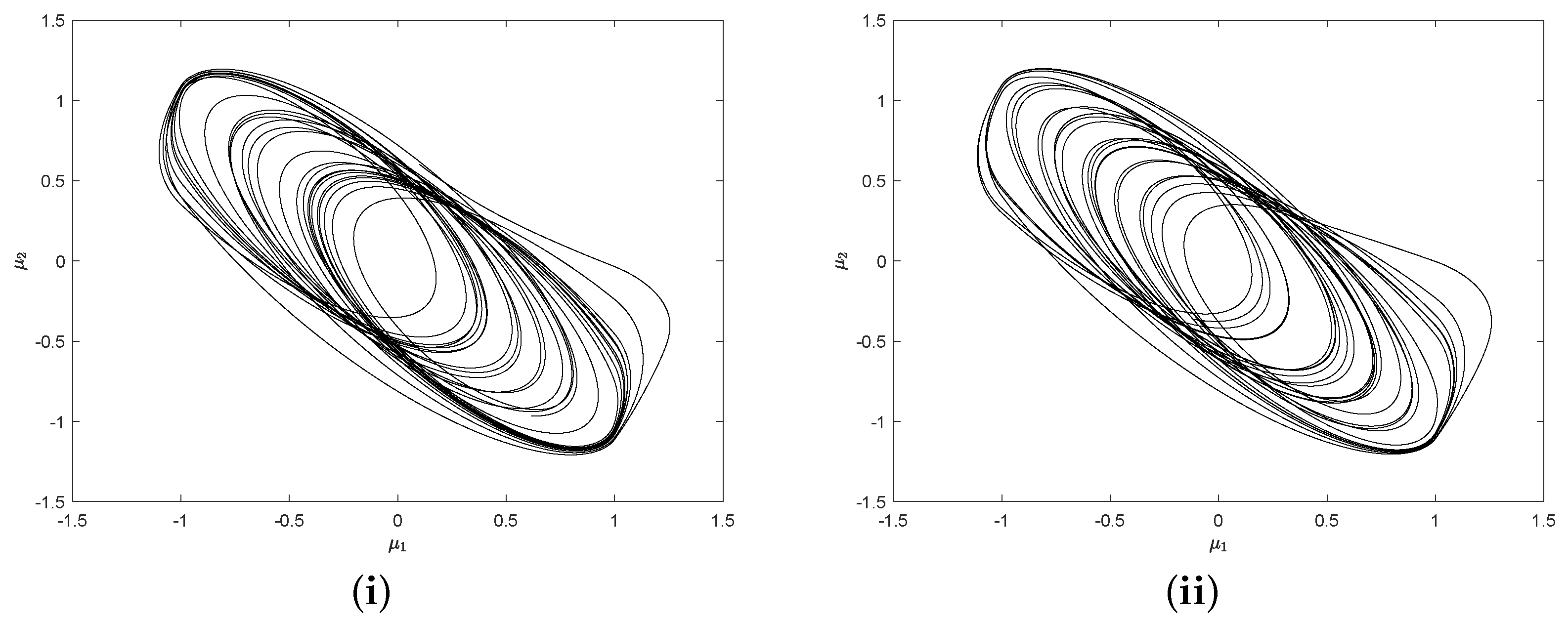
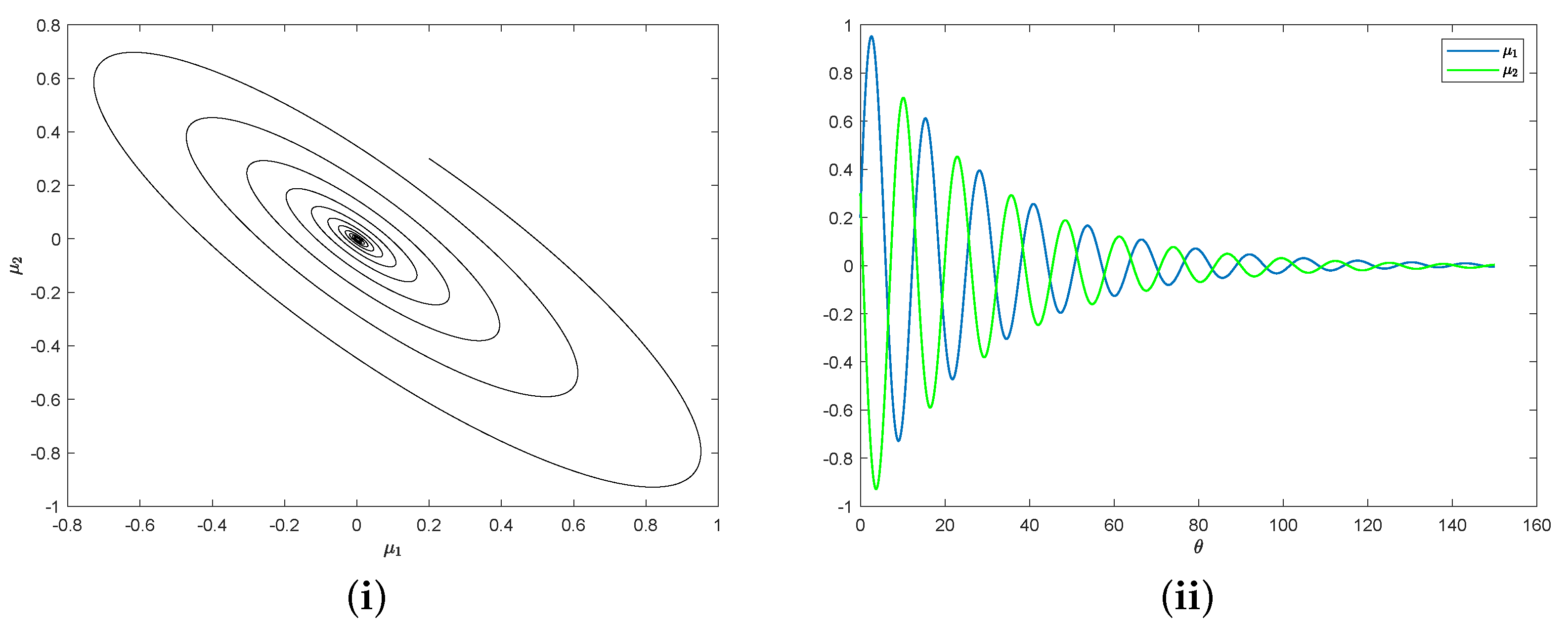
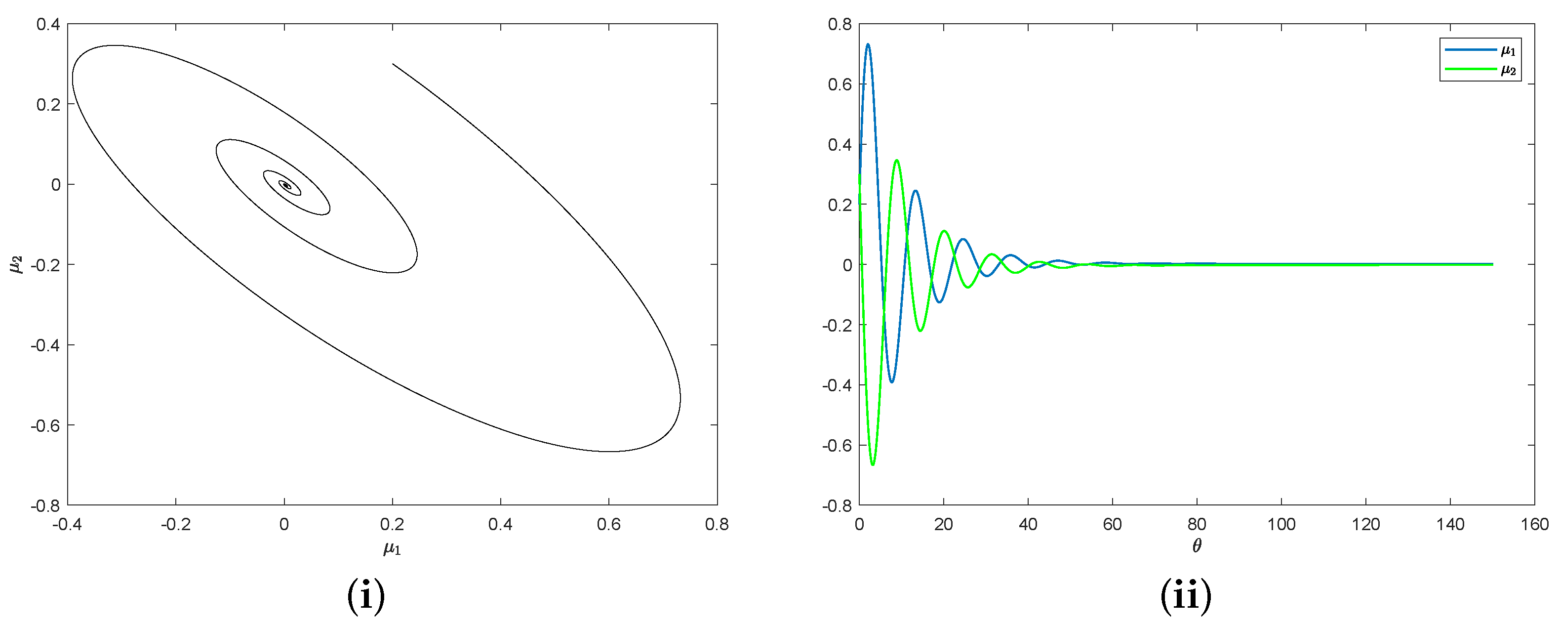
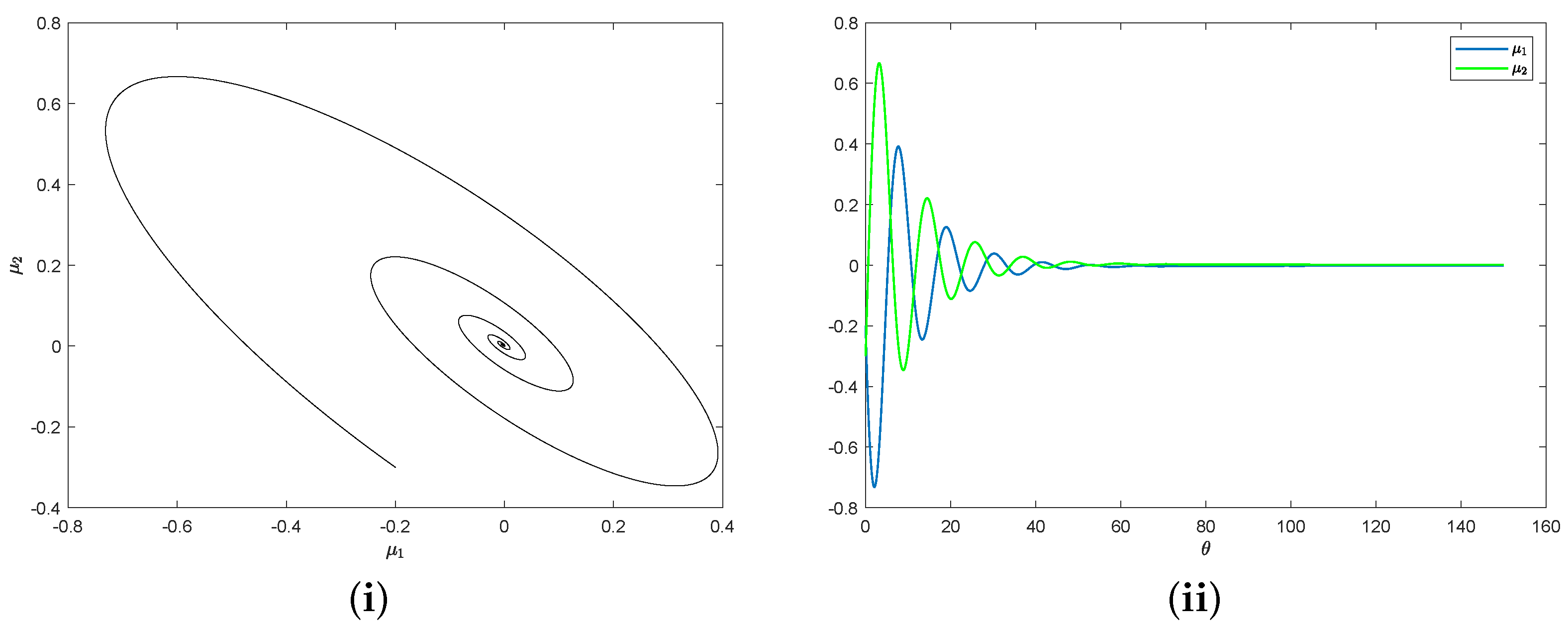
5. Application of a Non-Smooth System

To verify the correctness of our results, we took the modified MLC fractional-order circuit system as an example and simulated it. Under different parameter conditions, the dynamic behavior of modified MLC integer-order circuit systems is very rich [49,50].

The mathematical model of the modified MLC fractional-order circuit system is as follows (5). The model is the result of the dimensionless processing of the original state system, where $a_1$, $a_2$, b, f, and $\omega$ are a set of given parameters. f and $\omega$ are the amplitude and frequency of the external periodic force of the system. For the specific physical meanings of all parameters, please refer to [49,50].

$$\begin{array}{c}\hfill \left\{\begin{array}{c}{}_0^C{D}_{\theta }^{\eta }{\mu }_1={\mu }_2+H\left({\mu }_1\right)\hfill \\ {}_0^C{D}_{\theta }^{\eta }{\mu }_2=-{\mu }_1-(a_1+a_2){\mu }_2+fsin\left(\omega \theta \right)\hfill \end{array}\right.\end{array}$$

(5)

and

$$\begin{array}{c}\hfill H\left({\mu }_1\right)=\left\{\begin{array}{cc}(b-c){\mu }_1+c,\hfill & {\mu }_1>1\hfill \\ b{\mu }_1,\hfill & -1\le {\mu }_1\le 1\hfill \\ (b-c){\mu }_1-c,\hfill & {\mu }_1<-1\hfill \end{array}\right.\end{array}$$

The function $H\left({\mu }_1\right)$ is piecewise, so the system (5) is non-smooth. The switch boundaries ${\mu }_1=-1$ and ${\mu }_1=1$ divide ${\mathbb{R}}^2$ into three units:

$$\begin{array}{cc}\hfill & B_{+}=\left\{({\mu }_1,{\mu }_2)|{\mu }_1>1\right\}\hfill \\ \hfill & B_0=\left\{({\mu }_1,{\mu }_2)|-1\le {\mu }_1\le 1\right\}\hfill \\ \hfill & B_{-}=\left\{({\mu }_1,{\mu }_2)|{\mu }_1<-1\right\}\hfill \end{array}$$

To sum up, the piecewise differential Equation (5) can be represented by the following differential inclusion. In this case, $\mathcal{F}(\theta ,\mu )$ is a piecewise function in a single-valued map.

$$\begin{array}{c}\hfill {}_0^C{D}_{\theta }^{\eta }\mu \in \mathcal{F}(\theta ,\mu )=\left\{\begin{array}{c}{h}_1(\theta ,\mu ),\mu \in B_{+}\hfill \\ h_2(\theta ,\mu ),\mu \in B_0\hfill \\ h_3(\theta ,\mu ),\mu \in B_{-}\hfill \end{array}\right.\end{array}$$

$$h_1(\theta ,\mu )=\left(\begin{array}{c}{\mu }_2+(b-c){\mu }_1+c\\ -{\mu }_1-(a_1+a_2){\mu }_2+fsin\left(\omega \theta \right)\end{array}\right)$$

$$h_2(\theta ,\mu )=\left(\begin{array}{c}{\mu }_2+b{\mu }_1\\ -{\mu }_1-(a_1+a_2){\mu }_2+fsin\left(\omega \theta \right)\end{array}\right)$$

$$h_3(\theta ,\mu )=\left(\begin{array}{c}{\mu }_2+(b-c){\mu }_1-c\\ -{\mu }_1-(a_1+a_2){\mu }_2+fsin\left(\omega \theta \right)\end{array}\right)$$

Let us briefly verify the existence of Equation (5) on $\Delta =[0,T]$ for the initial value $\mu \left(0\right)={\mu }_0$, where ${\mu }_0\in {\mathbb{R}}^2$, $T>0$. Since $\mathcal{F}$ is continuous with respect to t and piecewise continuous with respect to $\mu$, $\mathcal{F}$ satisfies (D1). To prove that $\mathcal{F}$ satisfies (D2), we need to prove that $\mathcal{F}$ satisfies (D2) in different units. For $\mu \in B_{+}$,

$$\begin{array}{cc}\hfill \left|h_1(\theta ,\mu )\right|& \le \sqrt{{({\mu }_2+(b-c){\mu }_1+c)}^2+{(-{\mu }_1-(a_1+a_2){\mu }_2+fsin\left(\omega \theta \right))}^2}\hfill \\ \hfill & \le \left|{\mu }_2+(b-c){\mu }_1+c\right|+\left|(-{\mu }_1-(a_1+a_2){\mu }_2+fsin\left(\omega \theta \right))\right|\hfill \\ \hfill & \le \left|{\mu }_2\right|+\left|b-c\right|\left|{\mu }_1\right|+\left|c\right|+\left|{\mu }_1\right|+\left|a_1+a_2\right|\left|{\mu }_2\right|+\left|f\right|\hfill \\ \hfill & \le [\left|a_1+a_2\right|+1]\left|{\mu }_2\right|+[\left|b-c\right|+1]\left|{\mu }_1\right|+\left|f\right|+\left|c\right|\hfill \\ \hfill & \le [\left|a_1+a_2\right|+1]\sqrt{{{\mu }_1}^2+{{\mu }_2}^2}+[\left|b-c\right|+1]\sqrt{{{\mu }_1}^2+{{\mu }_2}^2}+\left|f\right|+\left|c\right|\hfill \\ \hfill & \le 2max\left\{\left|a_1+a_2\right|+1,\left|b-c\right|+1\right\}\left|\mu \right|+\left|f\right|+\left|c\right|\hfill \end{array}$$

Let $\rho \left(\theta \right)=2max\left\{\left|a_1+a_2\right|+1,\left|b-c\right|+1\right\}$, $\varphi \left(\theta \right)=\left|f\right|+\left|c\right|$; then, $\left|h_1(\theta ,\mu )\right|\le \rho \left(\theta \right)\left|\mu \right|+\varphi \left(\theta \right)$.

In the same way, it can be easily verified that

$$\left|h_2(\theta ,\mu )\right|\le \rho \left(\theta \right)\left|\mu \right|+\varphi \left(\theta \right),\left|h_3(\theta ,\mu )\right|\le \rho \left(\theta \right)\left|\mu \right|+\varphi \left(\theta \right).$$

Therefore, for $\forall {\mu }_0\in {\mathbb{R}}^2$, the existence of solutions of (5) on $\Delta$ has been verified according to Theorem 1.

If we use Theorem 2 to verify the existence of solutions of (5), we will obtain a weaker result. The process is as follows.

Let $a=a_1+a_2$, $\mu$, ${\mu }^{*}\in {\mathbb{R}}^n$, $\mu =({\mu }_1,{\mu }_2)$, ${\mu }^{*}=({\mu }_1^{*},{\mu }_2^{*})$, and $z_1={\mu }_1-{\mu }_1^{*}$, $z_2={\mu }_2-{\mu }_2^{*}$.

$$\begin{array}{cc}\hfill {\mathcal{H}}_d(\mathcal{F}(\theta ,\mu ),\mathcal{F}(\theta ,{\mu }^{*}))& =\left|\mathcal{F}(\theta ,\mu )-\mathcal{F}(\theta ,{\mu }^{*})\right|\hfill \\ \hfill & =\sqrt{{[{\mu }_2-{\mu }_2^{*}+H\left({\mu }_1\right)-H\left({\mu }_1^{*}\right)]}^2+{[-{\mu }_1+{\mu }_1^{*}-a{\mu }_2+a{\mu }_2^{*}]}^2}\hfill \\ \hfill & \le \left|z_2+H\left({\mu }_1\right)-H\left({\mu }_1^{*}\right)\right|+\left|-z_1-a{z}_2\right|\hfill \end{array}$$

For the piecewise function $H\left({\mu }_1\right)-H\left({\mu }_1^{*}\right)$, we have the following discussion.

When $-1\le {\mu }_1\le 1$, $H\left({\mu }_1\right)=b{\mu }_1=(b-c){\mu }_1+c{\mu }_1$. Then, for $H\left({\mu }_1\right)-H\left({\mu }_1^{*}\right)$, we have the following result.

$$\begin{array}{cc}\hfill H\left({\mu }_1\right)-H\left({\mu }_1^{*}\right)& =\left\{\begin{array}{c}(b-c)z_1+c({\mu }_1-1)\hfill \\ (b-c)z_1+c{z}_1\hfill \\ (b-c)z_1+c({\mu }_1+1)\hfill \end{array}\right.\hfill \\ \hfill & \le \left\{\begin{array}{c}(b-c)z_1+\left|c\right|\left|{\mu }_1-1\right|\hfill \\ (b-c)z_1+\left|c\right|\left|z_1\right|\hfill \\ (b-c)z_1+\left|c\right|\left|{\mu }_1+1\right|\hfill \end{array}\right.\hfill \\ \hfill & \le \left\{\begin{array}{cc}(b-c)z_1+\left|c\right|\left|{\mu }_1-{\mu }_1^{*}\right|,\hfill & {\mu }_1^{*}>1\hfill \\ (b-c)z_1+\left|c\right|\left|z_1\right|,\hfill & -1\le {\mu }_1^{*}\le 1\hfill \\ (b-c)z_1+\left|c\right|\left|{\mu }_1-{\mu }_1^{*}\right|,\hfill & {\mu }_1^{*}<-1\hfill \end{array}\right.\hfill \end{array}$$

Therefore, $H\left({\mu }_1\right)-H\left({\mu }_1^{*}\right)\le (b-c)z_1+\left|c\right|\left|z_1\right|$. For ${\mu }_1>1$ or ${\mu }_1<-1$, we can obtain the same result in the same way.

Thus,

$$\begin{array}{cc}\hfill {\mathcal{H}}_d(\mathcal{F}(\theta ,\mu ),\mathcal{F}(\theta ,{\mu }^{*}))& \le (\left|a\right|+1)\left|z_2\right|+(\left|b-c\right|+\left|c\right|+1)\left|z_1\right|\hfill \\ \hfill & \le [\left|a\right|+1+\left|b-c\right|+\left|c\right|+1]\sqrt{{z_1}^2+{z_2}^2}\hfill \end{array}$$

Let $l\left(\theta \right)=\left|a\right|+1+\left|b-c\right|+\left|c\right|+1$, then ${\mathcal{H}}_d(\mathcal{F}(\theta ,\mu ),\mathcal{F}(\theta ,{\mu }^{*}))\le l\left(\theta \right)\left|\mu -{\mu }^{*}\right|$. According to Theorem 2, for $\forall {\mu }_0\in {\mathbb{R}}^2$, there exists a solution of (5) on $[0,T^{\prime }]$, where $0<T^{\prime }<\Gamma (\eta +1)/\phantom{\Gamma (\eta +1)l_0}{l}_0$ and $d(0,\mathcal{F}(\theta ,0\left)\right)\le l\left(\theta \right)$ a.e. on $[0,T^{\prime }]$. This is obviously a weaker result with respect to the existence interval of solutions of (5) for $\forall {\mu }_0\in {\mathbb{R}}^2$. This is because when $\mathcal{F}$ satisfies both (D1) and (D3), (D4) is a more stringent condition than (D2).

Next, let us verify the uniqueness of solutions of (5) on $\Delta =[0,T]$ for the initial value $\mu \left(0\right)={\mu }_0$, where ${\mu }_0\in {\mathbb{R}}^2$, $T>0$. For $\mu$, ${\mu }^{*}\in {\mathbb{R}}^n$, and $h\in \mathcal{F}(\theta ,\mu )$, $h^{*}\in \mathcal{F}(\theta ,{\mu }^{*})$, we have

$$\begin{array}{cc}\hfill & \langle \mu -{\mu }^{*},h-h^{*}\rangle \hfill \\ \hfill & =\left({\mu }_1-{\mu }_1^{*},{\mu }_2-{\mu }_2^{*}\right){\left({\mu }_2-{\mu }_2^{*}+H\left({\mu }_1\right)-H\left({\mu }_1^{*}\right),-{\mu }_1+{\mu }_1^{*}-a{\mu }_2+a{\mu }_2^{*}\right)}^T\hfill \\ \hfill & \le \left(z_1,z_2\right){\left(z_2+H\left({\mu }_1\right)-H\left({\mu }_1^{*}\right),-z_1-a{z}_2\right)}^T\hfill \\ \hfill & =z_1{z}_2+z_1[H\left({\mu }_1\right)-H\left({\mu }_1^{*}\right)]-z_1{z}_2-a{z_2}^2\hfill \\ \hfill & \le \left|z_1\right|(\left|b-c\right|\left|z_1\right|+\left|c\right|\left|z_1\right|)+\left|a\right|{z_2}^2\hfill \\ \hfill & =\left|b-c\right|{z_1}^2+\left|c\right|{z_1}^2+\left|a\right|{z_2}^2\hfill \\ \hfill & \le max\{\left|b-c\right|+\left|c\right|,\left|a\right|\}({z_1}^2+{z_2}^2)\hfill \end{array}$$

Let $l=max\{\left|b-c\right|+\left|c\right|,\left|a\right|\}$; then, $\langle \mu -{\mu }^{*},h-h^{*}\rangle \le l{\left|\mu -{\mu }^{*}\right|}^2$.

According to Theorem 3, for $\forall {\mu }_0\in {\mathbb{R}}^2$, the uniqueness of solutions of (5) on $\Delta$ can be verified.

Finally, we simulate the system with four sets of selected parameters for $\eta =0.9$. This will serve as an auxiliary validation of the above. The software used for the simulation was Matlab. See [51,52] for the numerical algorithm used in our simulation.

In Figure 1, we can see that the system seems to be chaotic. This appears to indicate that the dynamic behavior of the system is also present in the fractional case.

In the integer-order modified MLC circuit system, when the parameters in Figure 2 are used, there is a stable limit cycle in the system [49]. When the parameters in Figure 3 or Figure 4 are used, the system exhibits periodic motion centered at $(0,0)$. However, from Figure 4, there is no stable limit cycle when $\eta =0.9$. From Figure 3 and Figure 4, there seems to be a stable equilibrium point $(0,0)$ when $\eta =0.9$. Regarding this difference, we have the following analysis.

Let $a=a_1+a_2$. When $f=0$, the Jacobian matrix of the circuit system at point (0, 0) is as follows:

$$J=\left[\begin{array}{cc}b& 1\\ -1& -a\end{array}\right]$$

Therefore, its characteristic equation is ${\lambda }^2+(a-b)\lambda +(1-ab)=0$. Thus, its two characteristic roots are ${\lambda }_{\pm }=[-(a-b)\pm \sqrt{{(a-b)}^2-4(1-ab)}]/2$. By the Hurwitz criterion, if the following conditions (6) hold, the characteristic roots ${\lambda }_{\pm }$ have a negative real part, i.e., $\left|arg|{\lambda }_{\pm }|\right|>\frac{\pi }{2}$.

$$(a-b)>0,\left|\begin{array}{cc}(a-b)& 1\\ 0& (1-ab)\end{array}\right|>0.$$

(6)

Therefore, when $a>b,ab<1$, in the case of the integer order, the equilibrium point $(0,0)$ is locally asymptotically stable.

In the case of the fractional order, the condition for the local asymptotic stability of the equilibrium point $(0,0)$ is $\left|arg|{\lambda }_{\pm }|\right|>\frac{\eta }{2}\pi$ [53]. Obviously, the Hurwitz conditions (6) can also ensure the stability of the equilibrium point (0, 0) in this case. For $(a-b)<0,{(a-b)}^2-4(1-ab)<0$, the above two characteristic roots can be written as ${\lambda }_{\pm }=[-(a-b)\mp i\sqrt{4(1-ab)-{(a-b)}^2}]/2$. Thus, we have the following conditions (7):

$$\begin{array}{cc}\hfill & (a-b)<0,{(a-b)}^2-4(1-ab)<0,\hfill \\ \hfill & |{tan}^{-1}\left(\sqrt{4(1-ab)-{\left((a-b)\right)}^2}\right)/(a-b)|>\eta \pi /2.\hfill \end{array}$$

(7)

Therefore, when conditions (6) or (7) hold, in the case of the fractional order, the equilibrium point $(0,0)$ is locally asymptotically stable.

6. Conclusions

In the study of initial value problems of Caputo fractional differential inclusion, we obtain the existence results for the case of convex and non-convex multivalued maps. The nonlinear Leray–Schauder-type alternative for compact Kakutani maps is the foundation for the proof of the convex case, and a generalized Gronwall inequality plays a key role in the application of the fixed point theorem. The proof of the non-convex case is based on the fixed point theorem for a contraction multi-valued map. Depending on an inequality of the Caputo fractional derivative with respect to the inner product, we obtained the uniqueness results corresponding to both the convex and non-convex cases. Finally, we applied our results to a fractional non-smooth system—the modified MLC fractional-order circuit system. Further, we simulated the circuit system with four different sets of parameters and focused on the implications of the simulation results for $f=0$.

References

1. Kilbas, A.A.; Srivastava, H.M.; Trujillo, J.J. Theory and Applications of Fractional Differential Equations; Elsevier: Amsterdam, The Netherlands, 2006. [Google Scholar]
2. Tepljakov, A. Fractional-order Modeling and Control of Dynamic Systems; Springer: Cham, Switzerland, 2017. [Google Scholar]
3. Yang, X.J.; Gao, F.; Yang, J. General Fractional Derivatives with Applications in Viscoelasticity; Academic Press: Cambridge, MA, USA, 2020. [Google Scholar]
4. Tarasov, V.E. Mathematical economics: Application of fractional calculus. Mathematics 2020, 8, 660. [Google Scholar] [CrossRef]
5. Daftardar-Gejji, V. Fractional Calculus and Fractional Differential Equations; Springer: Singapore, 2019. [Google Scholar]
6. Anastassiou, G.A. Advanced ordinary and fractional approximation by positive sublinear operators. Filomat 2021, 35, 1899–1913. [Google Scholar] [CrossRef]
7. Khan, Z.A.; Ahmad, I.; Shah, K. Applications of fixed point theory to investigate a system of fractional order differential equations. J. Funct. Space 2021. [Google Scholar] [CrossRef]
8. Bagley, R.L.; Calico, R.A. Fractional order state equations for the control of viscoelastic damped structures. J. Guid. Control Dyn. 1991, 14, 304–311. [Google Scholar] [CrossRef]
9. Toledo-Hernandez, R.; Rico-Ramirez, V.; Iglesias-Silva, G.A.; Diwekar, U.M. A fractional calculus approach to the dynamic optimization of biological reactive systems. Part I: Fractional models for biological reactions. Chem. Eng. Sci. 2014, 117, 217–228. [Google Scholar] [CrossRef]
10. Zhou, Y. Fractional Evolution Equations and Inclusions: Analysis and Control; Academic Press: Cambridge, MA, USA, 2016. [Google Scholar]
11. Petráš, I. Fractional-Order Nonlinear Systems: Modeling, Analysis and Simulation; Springer: New York, NY, USA, 2011. [Google Scholar]
12. Lakshmikantham, V.; Vatsala, A.S. Basic theory of fractional differential equations. Nonlinear-Anal.-Theory Methods Appl. 2008, 69, 2677–2682. [Google Scholar] [CrossRef]
13. Diethelm, K.; Ford, N.J. Analysis of Fractional Differential Equations. J. Math. Anal. Appl. 2002, 265, 229–248. [Google Scholar] [CrossRef] [Green Version]
14. Wang, F. Existence and Uniqueness of Solutions for a Nonlinear Fractional Differential Equation. J. Appl. Math. Comput. 2012, 39, 53–67. [Google Scholar] [CrossRef]
15. Gambo, Y.Y.; Ameen, R.; Jarad, F.; Abdeljawad, T. Existence and uniqueness of solutions to fractional differential equations in the frame of generalized Caputo fractional derivatives. Adv. Differ. Equ. 2018, 2018, 1–13. [Google Scholar] [CrossRef] [Green Version]
16. Diethelm, K. The Analysis of Fractional Differential Equations: An Application-Oriented Exposition Using Differential Operators of Caputo Type; Springer: Berlin, Germany, 2011. [Google Scholar]
17. Podlubny, I. Geometric and physical interpretation of fractional integration and fractional differentiation. Fract. Calc. Appl. Anal. 2002, 5, 367–386. [Google Scholar]
18. Clarke, F.H.; Ledyaev, Y.S.; Stern, R.J.; Wolenski, P.R. Nonsmooth Analysis and Control Theory; Springer Science & Business Media: Berlin/Heidelberg, Germany, 2008. [Google Scholar]
19. Bergounioux, M.; Bourdin, L. Pontryagin maximum principle for general Caputo fractional optimal control problems with Bolza cost and terminal constraints. ESAIM-Control OPtim. Calc. Var. 2020, 26, 35. [Google Scholar] [CrossRef]
20. Gomoyunov, M.I. Extremal shift to accompanying points in a positional differential game for a fractional-order system. Proc. Steklov Inst. Math. 2020, 308, 83–105. [Google Scholar] [CrossRef]
21. Kunze, M. Non-Smooth Dynamical Systems; Springer: Berlin/Heidelberg, Germany, 2000. [Google Scholar]
22. Smirnov, G.V. Introduction to the Theory of Differential Inclusions; American Mathematical Society: Providence, RI, USA, 2022. [Google Scholar]
23. Ahmad, B.; Alghanmi, M.; Alsaedi, A. A study of generalized caputo fractional differential equations and inclusions with steiltjes-type fractional integral boundary conditions via fixed-point theory. J. Appl. Anal. Comput 2021, 11, 1208–1221. [Google Scholar] [CrossRef] [PubMed]
24. Abbas, M.I.; Ragusa, M.A. Nonlinear fractional differential inclusions with non-singular Mittag-Leffler kernel. AIMS Math. 2022, 7, 20328–20340. [Google Scholar] [CrossRef]
25. Agarwal, R.P.; Benchohra, M.; Hamani, S. A survey on existence results for boundary value problems of nonlinear fractional differential equations and inclusions. Acta Appl. Math. 2010, 109, 973–1033. [Google Scholar] [CrossRef]
26. Cernea, A. A note on the existence of solutions for some boundary value problems of fractional differential inclusions. Fract. Calc. Appl. Anal. 2012, 15, 183–194. [Google Scholar] [CrossRef]
27. Nieto, J.J.; Ouahab, A.; Prakash, P. Extremal solutions and relaxation problems for fractional differential inclusions. Abstr. Appl. Anal. 2013, 2013. [Google Scholar] [CrossRef]
28. Kamenskii, M.; Obukhovskii, V.; Petrosyan, G.; Yao, J.C. Existence and approximation of solutions to nonlocal boundary value problems for fractional differential inclusions. Fixed Point Theory Appl. 2019, 2019, 1–21. [Google Scholar] [CrossRef] [Green Version]
29. Akdemir, A.O.; Karaoğlan, A.; Ragusa, M.A.; Set, E. Fractional integral inequalities via Atangana-Baleanu operators for convex and concave functions. J. Funct. Space 2021, 2021. [Google Scholar] [CrossRef]
30. İlhan, E. Analysis of the spread of Hookworm infection with Caputo-Fabrizio fractional derivative. Turk. J. Sci. 2022, 7, 43–52. [Google Scholar]
31. Liu, X.; Jia, B.G.; Erbe, L.; Peterson, A. Lyapunov Functions for fractional order h-difference systems. Filomat 2021, 35, 1155–1178. [Google Scholar] [CrossRef]
32. Beddani, M.; Hedia, B. Solution sets for fractional differential inclusions. J. Fract. Calc. Appl. 2019, 10, 273–289. [Google Scholar]
33. Cernea, A. On a fractional integro-differential inclusion of Caputo-Katugampola type. Bull. Math. Anal. Appl. 2019, 11, 22–27. [Google Scholar]
34. Gomoyunov, M.I. To the theory of differential inclusions with Caputo fractional derivatives. Differ. Equ. 2020, 56, 1387–1401. [Google Scholar] [CrossRef]
35. Kamenskii, M.; Obukhovskii, V.; Petrosyan, G.; Yao, J.C. On the Existence of a Unique Solution for a Class of Fractional Differential Inclusions in a Hilbert Space. Mathematics 2021, 9, 136. [Google Scholar] [CrossRef]
36. Deimling, K. Multivalued Differential Equations; Walter De Gruyter: Berlin, Germany, 1992. [Google Scholar]
37. Hu, S. Handbook of Multi-Valued Analysis, Volume I: Theory; Kluwer: Dordrecht, The Netherlands, 1997. [Google Scholar]
38. Aubin, J.P.; Frankowska, H. Set-Valued Analysis; Birkhauser: Boston, MA, USA, 1990. [Google Scholar]
39. Dzherbashian, M.M.; Nersesian, A.B. Fractional derivatives and Cauchy problem for differential equations of fractional order. Fract. Calc. Appl. Anal. 2020, 23, 1810–1836. [Google Scholar] [CrossRef]
40. Podlubny, I. Fractional Differential Equations. Mathematics in Science and Engineering; Academic Press: New York, NY, USA, 1999. [Google Scholar]
41. Samko, S.G.; Kilbas, A.A.; Marichev, O.I. Fractional Integrals and Derivatives; Gordon and Breach Science Publishers: Yverdon, Switzerland, 1993. [Google Scholar]
42. Chang, Y.K.; Li, W.T. Existence results for second order impulsive functional differential inclusions. J. Math. Anal. Appl. 2005, 301, 477–490. [Google Scholar] [CrossRef] [Green Version]
43. Covitz, H.; Nadler, S.B. Multi-Valued Contraction Mappings in Generalized Metric Spaces. Isr. J. Math. 1970, 8, 5–11. [Google Scholar] [CrossRef]
44. Granas, A.; Dugundji, J. Fixed Point Theory; Springer: New York, NY, USA, 2003. [Google Scholar]
45. Yosida, K. Functional Analysis, 6th ed.; Springer: Berlin, Germany, 1980. [Google Scholar]
46. Ye, H.; Gao, J.; Ding, Y. A generalized Gronwall inequality and its application to a fractional differential equation. J. Math. Anal. Appl. 2007, 328, 1075–1081. [Google Scholar] [CrossRef] [Green Version]
47. Castaing, C.; Valadier, M. Convex Analysis and Measurable Multifunctions; Springer: Berlin/Heidelberg, Germany, 1977. [Google Scholar]
48. Aguila-Camacho, N.; Duarte-Mermoud, M.A.; Gallegos, J.A. Lyapunov functions for fractional order systems. Commun. Nonlinear Sci. Numer. Simul. 2014, 19, 2951–2957. [Google Scholar] [CrossRef]
49. Fu, S.; Liu, Y. Complex Dynamical Behavior of Modified MLC Circuit. Chaos Solitons Fractals 2020, 141, 110–407. [Google Scholar] [CrossRef]
50. Srinivasan, K.; Chandrasekar, V.K.; Venkatesan, A.; Mohamed, I.R. Duffing–van der Pol oscillator type dynamics in Murali–Lakshmanan–Chua (MLC) circuit. Chaos Solitons Fractals 2016, 82, 60–71. [Google Scholar] [CrossRef]
51. Li, C.; Peng, G. Chaos in Chen’s systems with a fractional order. Chaos Solitons Fractals 2004, 22, 443–450. [Google Scholar] [CrossRef]
52. Zhou, P.; Huang, K. A new 4-D nonequilibrium fractional-order chaotic system and its circuit implementation. Commun. Nonlinear Sci. Numer. Simul. 2014, 19, 2005–2011. [Google Scholar] [CrossRef]
53. Ahmed, E.; El-Sayed, A.M.A.; El-Saka, H.A. On some Routh–Hurwitz conditions for fractional order differential equations and their applications in Lorenz, Rössler, Chua and Chen systems. Phys. Lett. A 2006, 358, 1–4. [Google Scholar] [CrossRef]
Figure 1. Phase diagram of the circuit system for a 1 = 1.00623 , a 2 = 0.00894 , b = 1.00621 , c = 2.93595 , f = 0.5272 , and ω = 0.843 ; (i) μ 0 = ( 0.1 , 0.6 ) ; (ii) μ 0 = ( 0.1 , 0.6 ) .
Mathematics 11 00653 g001
Figure 2. (i) Phase diagram of the circuit system for μ 0 = ( 0.2 , 0.3 ) , a 1 = 0.5 , a 2 = 0.3 , b = 0.9 , c = 2 , and f = 0 ; (ii) evolution of the state μ 1 , μ 2 .
Mathematics 11 00653 g002
Figure 3. (i) Phase diagram of the circuit system for μ 0 = ( 0.2 , 0.3 ) , a 1 = 0.5 , a 2 = 0.3 , b = 0.8 , c = 2 , and f = 0 ; (ii) evolution of the state μ 1 , μ 2 .
Mathematics 11 00653 g003
Figure 4. (i) Phase diagram of the circuit system for μ 0 = ( 0.2 , 0.3 ) , a 1 = 0.5 , a 2 = 0.3 , b = 0.8 , c = 2 , and f = 0 ; (ii) evolution of the state μ 1 , μ 2 .
Mathematics 11 00653 g004
Disclaimer/Publisher’s Note: The statements, opinions and data contained in all publications are solely those of the individual author(s) and contributor(s) and not of MDPI and/or the editor(s). MDPI and/or the editor(s) disclaim responsibility for any injury to people or property resulting from any ideas, methods, instructions or products referred to in the content.