Coordination of Plug-In Electric Vehicle Charging in a Stochastic Framework: A Decentralized Tax/Incentive-Based Mechanism to Reach Global Optimality ^†

Abstract

We address the problem of charging plug-in electric vehicles (PEVs) in a decentralized way and under stochastic dynamics affecting the real-time electricity tariff. The model is formulated as a Nash equilibrium seeking problem, where players wish to minimize the costs for charging their own PEVs. For finite PEVs populations, the Nash equilibrium does not correspond to the social optimum, i.e., to a control strategy minimizing the total electricity costs at the aggregate level. We accordingly introduce some taxes/incentives on the price of electricity for charging PEVs and show that it is possible to tune them so that (a) the social optimum is reached as a Nash equilibrium, (b) in correspondence with this equilibrium, players do not pay any net total tax, nor receive any net total incentive.

1. Introduction

In the transportation sector, plug-in electric vehicles (PEVs) are among the most promising alternatives to the exploitation of fossil fuels [1] and are expected to reach increasingly large market penetrations in the near future [2]. However, even moderate PEVs market penetrations may create new demand peaks in the electricity grid [3,4,5] and lead to serious issues concerning the grid stability [6]. Consequently, the need has emerged to coordinate the charging schedule of PEVs so as to mitigate the demand peaks, or to use the Energy, stored in the PEVs batteries as a source for providing ancillary services [7,8,9,10,11]. This proposal belongs, more generally, to the wider concept of demand-side management in smart grids. In order to regulate the charging of PEVs, centralized [12] as well as decentralized [13,14,15,16] approaches have been studied, the former approach being clearly less attractive in view of a real application. The decentralized approach typically relies on a game-theoretic framework and looks for Nash equilibria, where players cannot decrease their own costs by unilaterally changing their individual controls. The game describing the PEV problem falls within the class of aggregative games [17,18,19], where players are linked by a quantity depending on the sum of their controls. In recent years, a notable effort has been made to develop algorithms to compute or approximate Nash (or generalized Nash) equilibria in a decentralized or semi-decentralized way [20,21,22,23,24,25,26,27,28]. The PEV problem is among the most relevant applications of the above-cited decentralized algorithms (see e.g., [23,24,25,26,27]).

In this paper, we address a Nash-equilibrium-seeking problem for charging PEVs under stochastic dynamics and for a finite number of players. Players wish to minimize their own expected cost for charging PEVs, but at the same time, they must reach a full battery charge before the end of a given time interval. The curve describing the aggregate non-PEV demand for electricity is regulated by an underlying stochastic process. This, in turn, affects the real-time price of electricity, which is modeled as a function depending on the total instantaneous electricity demand. Building upon the model developed in [29], we employ the S-adapted information structure (firstly introduced in [30] and applied for instance in [31,32,33,34,35]) to describe the stochastic dynamics. More specifically, we assume that players can inspect in real-time the evolution of the stochastic process affecting the non-PEV demand, and accordingly adapt their charging controls. By contrast, players are not allowed to observe the other player’s actions. Several studies have already been devoted to the decentralized computation (or approximation) of Nash equilibria under stochastic dynamics (see e.g., [36,37,38,39,40,41]). However, as pointed out in [29], these papers are not concerned with the specific time dynamics and with the corresponding S-adapted information structure that is used in the present paper.

We show that, in the basic model discussed in this paper, the obtained Nash equilibria do not correspond to a social optimum, i.e., to a control curve minimizing the expectation value of the total (PEV and non-PEV), aggregate costs for electricity. This is a consequence of the finite number of players (see also [24,42]). In this case, indeed, single players are capable of affecting the price by modifying their charging controls alone, and can therefore steer the equilibrium towards a particular configuration they prefer, but which differs from a social optimum. To overcome this issue, we introduce some additional taxes/incentives on the price of electricity for charging PEVs, with the aim of recovering a socially optimal solution in correspondence with the Nash equilibrium (see for instance [43], however, in a slightly different context). We then show that such taxes/incentives are not uniquely defined, and analyze the possible options to tune them. As a main result of this paper, we show that it is possible to tune them so that the total tax (or incentive) that is paid (or received) is zero in correspondence with the Nash equilibrium. Remarkably enough, this holds true for any scenario realization of the stochastic process. As a consequence, we obtain a mechanism that allows the social optimum to be reached, but according to which, apart from the payment of the real cost of electricity, no additional money transfer is needed. More specifically, we formulate two variants of the proposed mechanism. In the first case, taxes/incentives are the same for all players, and the condition of zero total tax/incentive is valid at the aggregate level. In the second case, we allow taxes/incentives to be personalized for single players, and the condition of zero total tax/incentive is valid at the individual level.

The paper is structured as follows. In Section 2, we introduce the basic stochastic PEV problem and formulate it as a game involving N players. In Section 3, we introduce the concepts of Nash equilibrium and of social optimum in the context of our problem and show that, in general, they do not overlap. In Section 4, we discuss the proposal of modifying the game by adding some taxes or incentives on the price of electricity used for charging PEVs. Section 5 contains the main results of this paper; the additional taxes/incentives are tuned so as to achieve a vanishing total tax. A brief summary of the proposed mechanism is then described in Section 6. Finally, in Section 7, we discuss a simple numerical example in which the findings of this paper are applied.

Notation: We use boldface (e.g., $\mathit{u}$) to denote vectors. A notation of the type $\mathit{u}:=({\mathit{u}}_n;n\in \{1,\dots ,N\}):=({\mathit{u}}_1,\dots ,{\mathit{u}}_n)$, where ${\mathit{u}}_n\in {\mathbb{R}}^K$ and $\mathit{u}\in {\mathbb{R}}^{NK}$, is used to denote a collection of vectors (or scalars) into a larger vector. Given a function $J(\mathit{x},\mathit{y})$, where $\mathit{x}\in {\mathbb{R}}^K$, the gradient ${\nabla }_{\mathit{x}}J(\mathit{x},\mathit{y})$ is defined as the vector $\left({\partial }_{x_i}J(\mathit{x},\mathit{y});i\in \{1,\dots ,K\}\right)\in {\mathbb{R}}^K$. The Euclidean scalar product is denoted by $⟨·,·⟩$. We also use the following matrix notation: ${\mathbb{I}}_N$ is the identity $N\times N$ matrix, ${\mathbf{1}}_N$ is the column vector of length N whose elements are all equal to one, and finally, given a matrix X, $\sqrt{X}$ denotes its element-wise square root.

2. The Stochastic PEV Charging Problem

The problem studied in this paper is similar to the one discussed in [29] (see also [13,24]). N PEV batteries (possibly different in size) must be fully charged before the end of a given time interval $\mathcal{T}$. We will assume that $\mathcal{T}:=(1,\dots ,T)$ is divided into a set of T periods. As in [13,24,29], we use a real-time electricity tariff depending on the total instantaneous grid load, and model the problem as a game with N players, in which each player wishes to minimize the cost of charging her own PEV. We then look for PEV-charging controls $u_t$ that satisfy a Nash equilibrium of the game (see below for more details). Within our model, the non-PEV electricity demand of single players can be neither programmed nor predicted. However, at the aggregate level, we assume that the average non-PEV demand $d_t$ is actually known. To add some uncertainty, we include possible random fluctuations in the time-evolution of $d_t$, which in turn imply a stochastic dynamics affecting the electricity price. Following [29], we describe these dynamics by using an S-adapted information structure. This means that, during the evolution of the game, players are not assumed to inspect the other player’s actions, but can nevertheless observe the evolution of the stochastic process, i.e., they know the value of the average instantaneous non-PEV demand $d_t$.

Let us first introduce the notation describing the stochastic model. Given a probability space $(\Omega ,\mathfrak{F},\mathbb{P})$, the stochastic dynamics induces a natural filtration $\{\mathsf{\varnothing },\Omega \}\equiv {\mathfrak{F}}_1\subseteq {\mathfrak{F}}_2\dots \subseteq {\mathfrak{F}}_T$ of the $\sigma$-algebra $\mathfrak{F}$, where ${\mathfrak{F}}_T\subseteq \mathfrak{F}$. In this paper, the stochastic process is discrete, and the filtration can consequently be described by an event tree (see Figure 1) with K nodes and T periods. We denote by ${\mathcal{K}}_t\subseteq \mathcal{K}$ the set of all nodes corresponding to the time step $t\in \mathcal{T}$, where $\mathcal{K}$ is the set of all nodes in the event tree. To be more precise, ${\mathcal{K}}_1=\left\{k_1\right\}$ is made of the root node alone; the children nodes of $k_1$ define the set ${\mathcal{K}}_2$; in turn, all children nodes of the nodes in ${\mathcal{K}}_2$ define the set ${\mathcal{K}}_3$, and so on, until the leaf nodes ${\mathcal{K}}_T$ are reached. We use the notation $k_t$ to denote an arbitrary node belonging to ${\mathcal{K}}_t$, i.e., referring to the time step t. Furthermore, we define $\mathcal{A}\left(k_t\right)$ as the set containing the node $k_t$ and all of its ancestors. Notice that, for every node $k_t$, there is a unique path $\mathcal{A}\left(k_t\right)$ leading to $k_t$ from the root node $k_1$. Given a leaf node $k_T$, we call $\mathcal{A}\left(k_T\right)$ a sample path of the stochastic process. We use the letter S to indicate the number $|{\mathcal{K}}_T|$ of sample paths in the event tree. We further assume that, given any node $k_t\in \mathcal{K}$, the probability $P\left(k_t\right)$ that node $k_t$ is realized during period t is known in advance (we refer to [44] for more details about event trees in the S-adapted information structure).

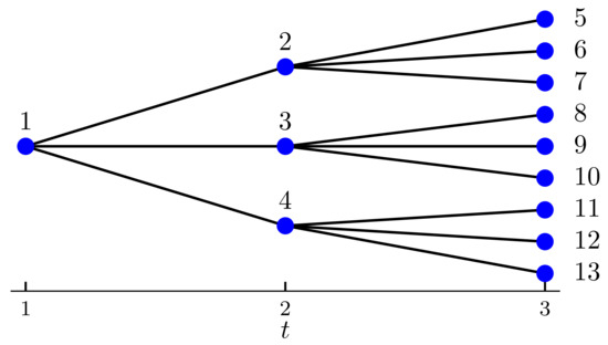
Figure 1. Example of an event tree with $T=3$ periods and $K=13$ nodes. According to the notation used in this paper, ${\mathcal{K}}_1=\left\{1\right\}$, ${\mathcal{K}}_2=\{2,3,4\}$ and ${\mathcal{K}}_3=\{5,\dots ,13\}$, where ${\mathcal{K}}_3\equiv {\mathcal{K}}_T$ is the set of leaf nodes. The tree contains $S=9$ sample paths, that is, $\mathcal{A}\left(5\right)=\{1,2,5\}$, $\mathcal{A}\left(6\right)=\{1,2,6\}$, $\mathcal{A}\left(7\right)=\{1,2,7\}$, $\mathcal{A}\left(8\right)=\{1,3,8\}$, $\mathcal{A}\left(9\right)=\{1,3,9\}$, $\mathcal{A}\left(10\right)=\{1,3,10\}$, $\mathcal{A}\left(11\right)=\{1,4,11\}$, $\mathcal{A}\left(12\right)=\{1,4,12\}$ and $\mathcal{A}\left(13\right)=\{1,4,13\}$.

The non-PEV demand of electricity on the node $k_t$ averaged for a single player is denoted by

$$d\left(k_t\right)>0.$$

(1)

Including the case of zero demand, $d\left(k_t\right)=0$, is, of course, possible, but would require the addition of a constant term in the price function $p(·)$ (see below) to avoid vanishing prices. To keep the notation simple, we prefer thus to define $d\left(k_t\right)$ as given by Equation (1).

Let $\mathcal{N}=\{1,\dots ,N\}$ be the set of players. To each node $k_t$, and for each player $n\in \mathcal{N}$, the control

$$u_n\left(k_t\right)\ge 0,\forall k_t\in \mathcal{K}$$

(2)

describes the amount of power used by player n to charge her own PEV battery on the node $k_t$ of the event tree. Notice that this formulation reflects nonanticipativity; indeed, for any $k_t$, the controls up to period t are clearly unique (and given by $\left\{u_n\left(k_{t^{\prime }}\right)\right|k_{t^{\prime }}\in \mathcal{A}\left(k_t\right)\}$) for every sample path passing through node $k_t$. This means that $u_n\left(k_t\right)$ only depends on the information gained up to the time step t, and therefore, nonanticipativity holds. We call the vector ${\mathit{u}}_n:=\left(\mathit{u}\left(k_t\right);k_t\in \mathcal{K}\right)\in {\mathbb{R}}^K$ collecting the controls of player n an S-adapted strategy for player n. The vector $\mathit{u}:=\left({\mathit{u}}_n;n\in \mathcal{N}\right)\in {\mathbb{R}}^{NT}$ collecting the controls of all players is simply called an S-adapted strategy. For the sake of consistency, a well-defined ordering of the nodes of $\mathcal{K}$ must of course be maintained in the definition of ${\mathit{u}}_n$ and $\mathit{u}$.

We can now describe the problem we are facing in a more precise way. For every node $k_t$, the aggregate control $\overline{u}\left(k_t\right)$ is defined as the average control over all players:

$$\overline{u}\left(k_t\right)=\frac{1}{N}\sum _{n\in \mathcal{N}}{u}_n\left(k_t\right).$$

(3)

Furthermore, for each node $k_t$ we consider an electricity tariff of the type

$$p\left(\frac{d\left(k_t\right)+\overline{u}\left(k_t\right)}{c}\right),$$

where $p(·)$ is a price function, and $c>0$ is the generation capacity averaged for a single player. For each player, the S-adapted cost function describes the expectation value of the cost for charging the PEV battery. Notice that we do not describe the total electricity cost for each player because, as mentioned, we consider the non-PEV electricity consumption of single players to be unpredictable. As discussed in [29], the S-adapted cost function for player n can be written as

$$J_n({\mathit{u}}_n,{\mathit{u}}_{-n}):=\sum _{k_t\in \mathcal{K}}P\left(k_t\right)p\left(\frac{d\left(k_t\right)+\overline{u}\left(k_t\right)}{c}\right)u_n\left(k_t\right),$$

(4)

where ${\mathit{u}}_{-n}:=\left({\mathit{u}}_m;m\in \mathcal{N},m\ne n\right)$ represents the collection of strategies of all players other than n.

As mentioned, each player wants to fully charge the battery before the end of the time interval $\mathcal{T}$. The state-of-charge of battery n in correspondence with node $k_t$ can be described by a number $x_n\left(k_t\right)$, such that $0\le x_n\left(k_t\right)\le 1$. More precisely, we use the following convention (notice that this convention differs from the one used in [29]): $x_n\left(k_t\right)$ is the state-of-charge at the end of the time step t, and at the beginning of the time step $t+1$. Requiring a full charge at the end of the time step T means that $x_n\left(k_T\right)=1$ for each leaf node $k_T$. Denoting by $0\le {\alpha }_n<1$ the charging efficiency and by ${\beta }_n>0$ the battery size, the time evolution of the state-of-charge is governed by the equation

$$x_n\left(k_t\right)=\left\{\begin{array}{c}{x}_{n,0}+\frac{{\alpha }_n}{{\beta }_n}{u}_n\left(k_t\right),t=1\hfill \\ x_n\left(a\left(k_t\right)\right)+\frac{{\alpha }_n}{{\beta }_n}{u}_n\left(k_t\right),1<t\le T,\hfill \end{array}\right.$$

(5)

where $x_{n,0}$ is the state-of-charge at the beginning of the time interval $\mathcal{T}$, and where $a\left(k_t\right)$ is the parent node of $k_t$. By repeatedly inserting Equation (5), we can formulate the full-charge requirement according to

$$1=x_{n,0}+({\alpha }_n/{\beta }_n)\sum _{k_t\in \mathcal{A}\left(k_T\right)}{u}_n\left(k_t\right),\forall k_T\in {\mathcal{K}}_T.$$

(6)

Notice that, for each player n, we are actually dealing with S distinct constraints (let us recall that $S\equiv |{\mathcal{K}}_T|$ is the number of different sample paths of the stochastic process). We can now define the feasibly set ${\mathcal{X}}_n\subseteq {\mathbb{R}}_{+}^K$ for player n as the set of S-adapted strategies ${\mathit{u}}_n$ satisfying Equations (2) and (6):

$$\begin{array}{cc}\hfill {\mathcal{X}}_n:=\{& {\mathit{u}}_n\in {\mathbb{R}}^K|u_n\left(k_t\right)\ge 0\forall k_t\in \mathcal{K},\hfill \\ \hfill & \sum _{k_t\in \mathcal{A}\left(k_T\right)}{u}_n\left(k_t\right)={\gamma }_n,\forall k_T\in {\mathcal{K}}_T\},\hfill \end{array}$$

(7)

where ${\gamma }_n:={\beta }_n(1-x_{n,0})/{\alpha }_n$. To model the players’ wish of minimizing their individual costs, we introduce the following game:

$$\mathcal{G}:=\left\{\begin{array}{cc}{\min }_{{\mathit{u}}_n}\hfill & J_n({\mathit{u}}_n,{\mathit{u}}_{-n})\hfill \\ \mathrm{s}.\mathrm{t}.\hfill & {\mathit{u}}_n\in {\mathcal{X}}_n\hfill \end{array}\right.\forall n\in \mathcal{N}$$

(8)

Notice that players are linked to one another by the price of electricity, which depends on the aggregate demand. In the next section, we will investigate game $\mathcal{G}$ in some more detail.

3. Nash Equilibrium vs. Social Optimum

We start by identifying some standard properties of the feasibility set ${\mathcal{X}}_n$.

 Proposition 1. 

The set ${\mathcal{X}}_n$ of feasible controls is nonempty, compact, and convex for any $n\in \mathcal{N}$. For $T>1$, it further satisfies Slater’s constraint qualification, i.e., its relative interior contains points for which $u_n\left(k_t\right)>0$

 Proof. 

The proof is straightforward. □

Let us now make some technical assumptions regarding the price function.

 Assumption 1. 

On the domain ${\mathbb{R}}_{+}$, the price function $p\left(x\right)$ is positive, convex, twice differentiable, has a strictly positive first derivative, and satisfies the following relation:

$$\frac{d^{2}p}{d{x}^2}(\alpha +x)\le \frac{2}{x}\frac{dp}{dx}(\alpha +x)$$

(9)

for any $\alpha \ge 0$.

This assumption is a proposal to relax the linear price function used, among others, in [24]. One can easily verify that, for instance, any function of the type $p\left(x\right)=a{x}^b$, with $a>0$ and $1\le b\le 3$, satisfies Assumption 1. As pointed out in [29], it may be possible to further relax this assumption to include a broader (and perhaps more simply defined) class of price functions. We leave this study for future research.

We can now proceed to define Nash equilibria (NE) of the game $\mathcal{G}$.

 Definition 1. 

A Nash equilibrium of the game $\mathcal{G}$ is an S-adapted strategy ${\mathit{u}}^{*}=({\mathit{u}}_1,\dots ,{\mathit{u}}_N)$ such that, for every player n, it is not possible to reduce the cost $J_n$ by only modifying the controls of player n:

$$J_n\left({\mathit{u}}_n^{*},{\mathit{u}}_{-n}^{*}\right)\le J_n\left({\mathit{u}}_n,{\mathit{u}}_{-n}^{*}\right),\forall {\mathit{u}}_n\in {\mathcal{X}}_n.$$

(10)

A Nash equilibrium of the game $\mathcal{G}$ can be found, according to the standard procedure, by solving the corresponding Variational Inequality. Defining the pseudogradient $\mathit{F}\left(\mathit{u}\right):=\left({\nabla }_{{\mathit{u}}_n}{J}_n({\mathit{u}}_n,{\mathit{u}}_{-n});n\in \mathcal{N}\right)\in {\mathbb{R}}^{NK}$, and letting $\mathcal{X}:={\mathcal{X}}_1\times \cdots \times {\mathcal{X}}_N\subseteq {\mathbb{R}}_{+}^{NK}$, the Variational Inequality is solved by the S-adapted strategy ${\mathit{u}}^{*}$ if

$$⟨\mathit{F}\left({\mathit{u}}^{*}\right),\mathit{u}-{\mathit{u}}^{*}⟩\ge 0,\forall \mathit{u}\in \mathcal{X}.$$

(11)

The following proposition is important to characterize the existence and uniqueness properties of solutions of the Variational Inequality (11).

 Proposition 2. 

Under Assumption 1, the pseudogradient $\mathit{F}\left(\mathit{u}\right)$ is strictly monotone on $\mathcal{X}$, i.e.,

$$⟨\mathit{F}\left(\mathit{u}\right)-\mathit{F}\left({\mathit{u}}^{\prime }\right),\mathit{u}-{\mathit{u}}^{\prime }⟩>0,\forall \mathit{u}\ne {\mathit{u}}^{\prime }\in \mathcal{X}.$$

(12)

The proof of Proposition 2 follows as the special case for $\lambda \left(k_t\right)=0$ of Proposition A1, and can be found in the Appendix A.

 Proposition 3. 

Under Assumption 1, the game $\mathcal{G}$ has a unique Nash equilibrium ${\mathit{u}}^{*}$, which is also the unique solution of the Variational Inequality (11).

 Proof. 

The proof is standard (see e.g., Theorems 1 and 2 in [45]) and relies on the fact that $\mathit{F}\left(\mathit{u}\right)$ is strictly monotone (Proposition 2). □

Let us now turn to a different kind of equilibrium. We consider this time the expectation value of the total (both PEV and non-PEV) cost for electricity averaged over all players, which is described by the cost function

$$\tilde{J}\left(\overline{\mathit{u}}\right):=\sum _{k_t\in \mathcal{K}}P\left(k_t\right)p\left(\frac{d\left(k_t\right)+\overline{u}\left(k_t\right)}{c}\right)(d\left(k_t\right)+\overline{u}\left(k_t\right)).$$

(13)

 Definition 2. 

A social optimum for the (stochastic) PEV charging problem is an S-adapted strategy $\mathit{u}**$ minimizing the total expected cost, i.e., for which

$$\tilde{J}\left(\overline{\mathit{u}}**\right)\le \tilde{J}\left(\overline{\mathit{u}}\right),\forall \mathit{u}\in \mathcal{X}.$$

(14)

Let us stress that, while we have included both PEV and non-PEV costs in the definition of the social optimum, the game $\mathcal{G}$ introduced above aims at the minimization of costs for charging PEV alone. From a global perspective, a social optimum clearly is the most desirable charging strategy. As shown by [13], in the deterministic case $S=1$ any social optimum of the PEV problem satisfies the valley-filling property, i.e.,

$${\overline{u}}_t^{**}=max\{0,\theta -d_t\}.$$

(15)

The valley-filling level $\theta$ is uniquely defined by (a) the shape of the non-PEV demand curve $d_t$ and (b) the total amount of power to be charged. In the S-adapted case, the valley-filling property is of course violated, since one is obliged to choose controls $u_n\left(k_t\right)$ before knowing the exact evolution of non-PEV demand, i.e., before that it is possible to calculate the valley-filling level $\theta$. In Figure 2, an example of a valley-filling charging profile is plotted (blue curve). The figure also shows an example of social optimum in a stochastic environment, which clearly violates the valley-filling condition (red, dash-dotted curve). The model is borrowed from Section 7, where it is discussed in detail. Here, let us just point out that the step-wise structure in the S-adapted total demand is due to the particular features of the example in question, which is piecewise deterministic.

At this point, it may be natural to wonder whether the Nash equilibrium of $\mathcal{G}$ is also a social optimum. The example plotted in Figure 3 (calculated again, for the sake of simplicity, within a deterministic framework) shows that this is, in general, not true. The main reason is due to the fact that the cost functions of $\mathcal{G}$ only reflect the costs for charging PEVs. In more detail, we may interpret the obtained Nash equilibria as follows: players realize that, by modifying their individual controls, they can affect the price. When $d_t$ is small and charging controls are large, they conclude that it is better to reduce the price by consuming a bit less than in the valley-filling solution. This implies that they must afford larger prices during other periods, where total demand rises above the valley-filling level. In these periods, however, charging controls are small, and the price increase has a smaller impact on the cost of charging PEV. In conclusion, the total aggregate demand $d_t+{\overline{u}}_t$ has a convex shape, as opposed to the flat, valley-filling solution. The figure suggests, however, that the valley-filling social optimum is reached in the case $N\to \infty$. When N is large, indeed, individual charging controls have almost no effect on the price of electricity. If during a given period, prices were sufficiently low, individual players would be incentivized to exploit this favorable condition by charging as much as possible during the period in question, and at the same time believing that price would stay almost unaffected. Since the same reasoning is made by all players, however, the total aggregate demand tends to get levelized, and a valley-filling equilibrium is approached. The convergence of the Nash equilibrium of $\mathcal{G}$ towards the valley-filling solution for $N\to \infty$ is proven in [13] in a framework very similar to the one presented here (see also [24,42]).

Figure 2. Two examples of aggregate control curve ${\overline{u}}_t^{**}$ solving the social optimum condition. The green, dashed curve describes the non-PEV demand, and follows the non-PEV demand curve $d^{\left(1\right)}$ introduced in Section 7. The blue curve represents total demand in the deterministic case and is valley-filling. The red, dash-dotted curve is calculated in a stochastic framework with the S-adapted information structure. It represents the total demand for the scenario realization corresponding to the depicted non-PEV demand curve $d_t$. Details about the numerical settings are discussed in Section 7. In particular, the stochastic curve is borrowed from the upper-left subplot in Figure 4.

Figure 2. Two examples of aggregate control curve ${\overline{u}}_t^{**}$ solving the social optimum condition. The green, dashed curve describes the non-PEV demand, and follows the non-PEV demand curve $d^{\left(1\right)}$ introduced in Section 7. The blue curve represents total demand in the deterministic case and is valley-filling. The red, dash-dotted curve is calculated in a stochastic framework with the S-adapted information structure. It represents the total demand for the scenario realization corresponding to the depicted non-PEV demand curve $d_t$. Details about the numerical settings are discussed in Section 7. In particular, the stochastic curve is borrowed from the upper-left subplot in Figure 4.

Figure 3. Examples of Nash equilibria of the game $\mathcal{G}$ for different numbers N of identical players. The thick blue curve corresponds to the (valley-filling) social optimum and is reached in the limit $N\to \infty$. Details about the game settings are discussed in Section 7; however, with the following differences: (a) the game evolution is deterministic, and follows the non-PEV demand curve $d^{\left(1\right)}$ introduced in Section 7; (b) players are homogeneous, and their parameters are equal to those of players 1–5 in the numerical example of Section 7.

Figure 3. Examples of Nash equilibria of the game $\mathcal{G}$ for different numbers N of identical players. The thick blue curve corresponds to the (valley-filling) social optimum and is reached in the limit $N\to \infty$. Details about the game settings are discussed in Section 7; however, with the following differences: (a) the game evolution is deterministic, and follows the non-PEV demand curve $d^{\left(1\right)}$ introduced in Section 7; (b) players are homogeneous, and their parameters are equal to those of players 1–5 in the numerical example of Section 7.

4. Social Optimum as the Nash Equilibrium of a Game with Taxes and Incentives

In this section, we address the question of whether it is possible to modify the game $\mathcal{G}$ in such a way that the Nash equilibrium corresponds to a social optimum ${\overline{\mathit{u}}}^{**}$. Let us consider the cost functions

$$\begin{array}{cc}\hfill & {\overline{J}}_n({\mathit{u}}_n,{\mathit{u}}_{-n};\mathit{\lambda }):=\hfill \\ \hfill & \sum _{k_t\in \mathcal{K}}P\left(k_t\right)\left(p\left(\frac{d\left(k_t\right)+\overline{u}\left(k_t\right)}{c}\right)+\lambda \left(k_t\right)\right)u_n\left(k_t\right)),\hfill \end{array}$$

(16)

where an additional tax or incentive $\lambda \left(k_t\right)$ has been added to the price of electricity used for charging PEVs. The idea is to calibrate $\lambda \left(k_t\right)$ so as to obtain a game whose Nash equilibrium ${\mathit{u}}^{*}$ is also a social optimum. Notice that, because of the $\lambda \left(k_t\right)$, the total costs afforded by players do not correspond anymore to Equation (13). It is possible to overcome this problem by redistributing the excess/missing costs by means of a lump-sum

$${\Lambda }_n\left(k_T\right)=\sum _{k_t\in \mathcal{A}\left(k_T\right)}\lambda \left(k_t\right)u_n^{*}\left(k_t\right),$$

(17)

so that the net tax paid by players is zero, and the social optimum defined in Equation (14) can still be interpreted as the aggregate control for which total costs are minimized.

We will now show that it is possible to define an extended game involving $\lambda \left(k_t\right)$ as additional controls so that the controls ${\mathit{\lambda }}^{*}$ at the equilibrium correspond to the sought taxes or incentives to achieve social optimality.

At first, we calculate the aggregate control ${\overline{\mathit{u}}}^{**}$ at the social optimum, by simply solving Equation (14) as a convex optimization problem. Notice that, given Assumption 1, the cost function $\tilde{J}\left(\overline{u}\right)$ is actually convex for $\mathit{u}\in \mathcal{X}$, as it is the product of two convex, nondecreasing, positive functions (see e.g., Exercise 3.32 in [46]). Let us now employ the formalism developed in [24] (and extended in [29] to the S-adapted case) to find generalized Nash equilibria in a distributed way. We consider a game ${\mathcal{G}}_{ext}$ with $N+1$ players, and with cost functions given by

$$\begin{array}{cc}\hfill J_n^{ext}(\mathit{u},\mathit{\lambda })& :={\overline{J}}_n(\mathit{u};\mathit{\lambda }),n\in \mathcal{N}\hfill \end{array}$$

(18)

$$\begin{array}{cc}\hfill J_{N+1}^{ext}(\mathit{u},\mathit{\lambda })& :=-\sum _{k_t\in \mathcal{K}}P\left(k_t\right)\lambda \left(k_t\right)\left(\sum _n{u}_n\left(k_t\right)-N{\overline{u}}^{**}\left(k_t\right)\right).\hfill \end{array}$$

(19)

Here, $\mathit{\lambda }:=(\lambda \left(k_t\right);k_t\in \mathcal{K})\in {\mathbb{R}}^K$ is the strategy of the additional player, which can be understood as a central regulator. The game is simply defined as

$${\mathcal{G}}_{ext}:=\left\{\begin{array}{cc}\underset{{\mathit{u}}_n\in {\mathcal{X}}_n}{min}\hfill & J_n^{ext}({\mathit{u}}_n,{\mathit{u}}_{-n},\mathit{\lambda }),\forall n\in \mathcal{N}\hfill \\ \underset{\mathit{\lambda }\in \mathbb{R}}{min}\hfill & J_{N+1}^{ext}(\mathit{u},\mathit{\lambda }).\hfill \end{array}\right.$$

(20)

 Proposition 4. 

Under Assumption 1, game ${\mathcal{G}}_{ext}$ admits the existence of a Nash equilibrium $({\mathit{u}}^{*},{\mathit{\lambda }}^{*})\in {\mathbb{R}}^{K(N+1)}$. Furthermore, the S-adapted strategy ${\mathit{u}}^{*}\in {\mathbb{R}}^{KN}$ at the Nash equilibrium is unique.

 Proof. 

Since the feasibility region for $\mathit{\lambda }\in \mathbb{R}$ is unbounded, one cannot infer the existence of the Nash equilibrium for ${\mathcal{G}}_{ext}$ as directly as it was achieved for Proposition 3. We formulate instead a generalized Nash equilibrium (GNE) seeking problem with feasibility set $\mathcal{U}:=\{\mathit{u}\in \mathcal{X}|{\sum }_n{u}_n\left(k_t\right)=N{\overline{u}}^{**}\left(k_t\right),\forall k_t\in \mathcal{K}\}\subset {\mathbb{R}}^{KN}$. The game reads

$${\mathcal{G}}_{GN}:=\left\{\begin{array}{cc}{\min }_{{\mathit{u}}_n}\hfill & J_n({\mathit{u}}_n,{\mathit{u}}_{-n}),\forall n\in \mathcal{N}\hfill \\ \mathrm{s}.\mathrm{t}.\hfill & \mathit{u}\in \mathcal{U}.\hfill \end{array}\right.$$

(21)

The set $\mathcal{U}$ is bounded and satisfies the standard technical assumptions mentioned in Proposition 1. As a consequence, according to [45], a specific generalized Nash equilibrium of ${\mathcal{G}}_{GN}$ (called a normalized equilibrium) exists and can be found by solving the Karush–Kuhn–Tucker (KKT) Equations (24)–(29). More precisely, several normalized GNE’s may exist. The equilibrium discussed here is obtained by setting to 1 the coefficients $r_n$ defined in [45]. Since the latter KKT conditions are equivalent to finding a Nash equilibrium of ${\mathcal{G}}_{ext}$, it is clear that a Nash equilibrium of ${\mathcal{G}}_{ext}$ exists. Moreover, [45] shows that the GNE of ${\mathcal{G}}_{GN}$ solving the KKT Equations (24)–(29) is unique. This is equivalent to the uniqueness of the controls ${\mathit{u}}^{*}$ at the Nash equilibrium of ${\mathcal{G}}_{ext}$ (notice that, by contrast, no uniqueness property is established for ${\mathit{\lambda }}^{*}$). □

It is clear that any Nash equilibrium $({\mathit{u}}^{*},{\mathit{\lambda }}^{*})$ of ${\mathcal{G}}_{ext}$ is a social optimum, i.e., satisfies the equality constraint

$$\overline{u}\left(k_t\right)={\overline{u}}^{**}\left(k_t\right),\forall k_t\in \mathcal{K}.$$

(22)

Indeed, if Equation (22) were violated at node $k_t$, the (N+1)-th player would try to choose a value of $\lambda \left(k_t\right)$ with $\left|\lambda \right(k_t\left)\right|\to \infty$, so that no equilibrium would be reached. We point out that, since Equation (22) is an equality constraint, the controls $\lambda \left(k_t\right)$ are allowed to be both positive or negative, and can thus be interpreted as taxes or incentives, respectively. This is a difference with respect to [24,29], where the coupling constraints are of the inequality type, and the multipliers $\lambda$ have to be nonnegative. This fact will play a major role in the following section, where a weighted sum of the parameters $\lambda \left(k_t\right)$ will be set equal to zero.

Furthermore, it is clear that the unique S-adapted strategy ${\mathit{u}}^{*}$ corresponds to the Nash equilibrium of the game

$${\mathcal{G}}_{mod}\left({\mathit{\lambda }}^{*}\right):=\left\{\begin{array}{cc}{\min }_{{\mathit{u}}_n}\hfill & {\overline{J}}_n({\mathit{u}}_n,{\mathit{u}}_{-n};{\mathit{\lambda }}^{*})\hfill \\ \mathrm{s}.\mathrm{t}.\hfill & {\mathit{u}}_n\in {\mathcal{X}}_n\hfill \end{array}\right.\forall n\in \mathcal{N},$$

(23)

which is equal to the original game $\mathcal{G}$, but with cost functions of the type given by Equation (16).

Let us make some comments about the results we have obtained so far:

• We have actually found the first possible way to calculate the correct taxes/incentives $\lambda \left(k_t\right)$ to achieve a social optimum. A Nash equilibrium of the extended game ${\mathcal{G}}_{ext}$ can indeed be obtained by solving the corresponding Variational Inequality. As we are going to propose a slightly different procedure for calculating $\lambda \left(k_t\right)$ in Section 5, we prefer here to omit further details about possible numerical methods to solve this Variational Inequality.
• At this stage, however, we have no control over the value of the lump-sum ${\Lambda }_n\left(k_T\right)$ that is redistributed or demanded by each player at the end of the game. If the lump-sum is large as compared to the cost reduction made possible by social optimality, the whole mechanism could be perceived negatively by players.
• The taxes/incentives ${\mathit{\lambda }}^{*}$ at the Nash equilibrium of ${\mathcal{G}}_{ext}$ are not expected to be unique. It may therefore be interesting to investigate whether it is possible to tune them to reduce the lump-sum. In the next section, we will show indeed that it is possible to choose ${\mathit{\lambda }}^{*}$ such that the aggregate lump-sum ${\sum }_n{\Lambda }_n\left(k_T\right)=0$ for each $k_T\in {\mathcal{K}}_T$. We will also propose a variant with personalized price/incentives ${\lambda }_n\left(k_t\right)$, and show that, in this case, the personalized lump-sum can be made to vanish individually for each player.

To be socially accepted, a system with tax/incentive must be egalitarian, i.e., everybody is treated the same way, and fair, i.e., the total tax/incentive must be zero. If all players are homogenous, equality and fairness are possible. If players are not homogenous, this can be partially attained and we have two cases depending if we put the priority on equality or fairness. In the first case, the tax/incentive should be the same for everybody even if the players are different (for example people and big firms should be treated the same way). The price to pay for this is that fairness is only valid at the aggregated level. In the second case, fairness is valid for each player. The price to pay for this is that the tax/incentive might differ. However, it is important to say that players with the same characteristics have the same tax/incentive.

5. Choosing the Level of Taxes/Incentives to Obtain a Vanishing Total Tax/Incentive

Finding a Nash equilibrium of ${\mathcal{G}}_{ext}$ is equivalent to solving the KKT equations

$$\begin{array}{cc}\hfill & \frac{\partial }{\partial u_n\left(k_t\right)}{J}_n+P\left(k_t\right)\lambda \left(k_t\right)+\sum _{k_T\in \mathcal{L}\left(k_t\right)}{\nu }_n\left(k_T\right)-{\mu }_n\left(k_t\right)=0,\hfill \end{array}$$

$$\begin{array}{cc}\hfill & \forall k_t\in \mathcal{K},n\in \mathcal{N}\hfill \end{array}$$

(24)

$$\begin{array}{cc}\hfill & \sum _n{u}_n\left(k_t\right)-N{\overline{u}}^{**}\left(k_t\right)=0,\forall k_t\in \mathcal{K}\hfill \end{array}$$

(25)

$$\begin{array}{cc}\hfill & {\mu }_n\left(k_t\right)\ge 0,\forall k_t\in \mathcal{K},n\in \mathcal{N}\hfill \end{array}$$

(26)

$$\begin{array}{cc}\hfill & u_n\left(k_t\right){\mu }_n\left(k_t\right)=0,\forall k_t\in \mathcal{K},n\in \mathcal{N}\hfill \end{array}$$

(27)

$$\begin{array}{cc}\hfill & u_n\left(k_t\right)\ge 0,\forall k_t\in \mathcal{K},n\in \mathcal{N}\hfill \end{array}$$

(28)

$$\begin{array}{cc}\hfill & \sum _{k_t\in \mathcal{A}\left(k_T\right)}{u}_n\left(k_t\right)={\gamma }_n,\forall k_T\in {\mathcal{K}}_T,n\in \mathcal{N},\hfill \end{array}$$

(29)

where ${\nu }_n\left(k_T\right)$ are the Lagrangian multipliers corresponding to the full-charge constraint (Equation (29)), and where ${\mu }_n\left(k_t\right)$ are the Lagrangian multipliers corresponding to the constraint of nonnegative controls (Equation (28)). In Equation (24), the set $\mathcal{L}\left(k_t\right):=\{k_T\in {\mathcal{K}}_T|k_t\in \mathcal{A}\left(k_T\right)\}$ is the set of leaf nodes having $k_t$ as common ancestor.

Assume now that the S-adapted strategy ${\mathit{u}}^{*}$ solves the KKT equations. We are going to show that, because of some redundancy in the constraints, the parameters $\lambda \left(k_t\right)$, ${\nu }_n\left(k_T\right)$ and ${\mu }_n\left(k_t\right)$ are not uniquely defined. We can indeed find transformations of these parameters that keep the solution ${\mathit{u}}^{*}$ invariant. Consider for instance the transformations

$$\begin{array}{cc}\hfill {\nu }_n\left(k_T\right)& \to {\nu }_n^{\prime }\left(k_T\right)={\nu }_n\left(k_T\right)+{\delta }_{\nu }\left(k_T\right)\hfill \end{array}$$

(30)

$$\begin{array}{cc}\hfill \lambda \left(k_t\right)& \to {\lambda }^{\prime }\left(k_t\right)=\lambda \left(k_t\right)-P{\left(k_t\right)}^{-1}\sum _{k_T\in \mathcal{L}\left(k_t\right)}{\delta }_{\nu }\left(k_T\right),\hfill \end{array}$$

(31)

which are determined by a set $\{{\delta }_{\nu }\left(k_T\right)\in \mathbb{R};k_T\in {\mathcal{K}}_T\}$ of S parameters. We can easily observe that these transformations leave Equation (24) unchanged. In the deterministic case ($S=1$), the transformation of ${\lambda }_t$ reduces to a constant shift ${\lambda }_t\to {\lambda }_t+{\delta }_{\lambda }$, which makes the redundancy between ${\lambda }_t$ and ${\nu }_n$ easy to be understood. Indeed, since players need to consume a well-defined amount of power before the end of the time interval (this is the constraint having ${\nu }_n$ as Lagrange parameters), it is clear that adding a constant term to the price will not change the player’s behavior. In light of this interpretation, we can also consider the transformation in the stochastic case, Equation (31), as the addition of S different constant terms to the price of electricity, one for each scenario. In addition to that, transformations of the type

$$\begin{array}{cc}\hfill {\mu }_n\left(k_t\right)& \to {\mu }_n^{\prime }\left(k_t\right)={\mu }_n\left(k_t\right)+{\delta }_{\mu }\left(k_t\right)\hfill \end{array}$$

(32)

$$\begin{array}{cc}\hfill {\lambda }^{\prime }\left(k_t\right)& \to {\lambda }^{″}\left(k_t\right)={\lambda }^{\prime }\left(k_t\right)+P{\left(k_t\right)}^{-1}{\delta }_{\mu }\left(k_t\right)\hfill \end{array}$$

(33)

can be performed for all nodes $k_t$ in which the charging controls of all players are identical to zero, i.e., in which ${\overline{u}}^{*}\left(k_t\right)=0$. Notice that, in order to preserve the validity of Equation (26), ${\delta }_{\mu }\left(k_t\right)$ must be in the range $[-{min}_n{\mu }_n\left(k_t\right),+\infty )$. We can interpret this transformation as follows: in the nodes where controls are already zero, increasing the price will obviously keep controls equal to zero, since controls must be nonnegative (this is the constraint having ${\mu }_n\left(k_T\right)$ as Lagrange parameters). Decreasing the price may keep the controls equal to zero as well, provided that the price decrease is sufficiently small.

5.1. Tuning the $\lambda$’s So That, at the Equilibrium, the Total Tax/Incentive Is Zero at the Aggregate Level

In this subsection, we show that it is possible to tune the $\lambda \left(k_t\right)$ in such a way that, at the equilibrium, the aggregate control ${\overline{u}}^{*}\left(k_t\right)$ does not pay any tax nor receives any incentive, i.e., ${\sum }_n{\Lambda }_n\left(k_T\right)=0$. As a quite remarkable result, this is true for any sample path $\mathcal{A}\left(k_T\right)$ of the tree. In order to perform the next calculations, it may be convenient to switch to a matrix and vector notation. In addition to the already defined vectors ${\nabla }_n{J}_n\left(\mathit{u}\right)\in {\mathbb{R}}^K$, ${\mathit{u}}_n\in {\mathbb{R}}^K$ and $\mathit{\lambda }\in {\mathbb{R}}^k$, we introduce ${\mathbf{\nu }}_n:=({\nu }_n\left(k_T\right);k_T\in {\mathcal{K}}_T)\in {\mathbb{R}}^S$, and ${\mathbf{\mu }}_n:=({\mu }_n\left(k_t\right);k_t\in \mathcal{K})\in {\mathbb{R}}^K$. All vectors defined here are intended to be column vectors. We also denote by $P\in {\mathbb{R}}^{K\times K}$ the diagonal matrix having all node probabilities $P\left(k_t\right)$ on the diagonal, and by ${\overline{U}}^{*}$ the diagonal matrix having the aggregate controls ${\overline{\mathit{u}}}^{*}$ on the diagonal. Moreover, we introduce the incidence matrix $B\in {\mathbb{R}}^{K\times S}$, with elements $B_{ij}=1$ if the sample path indexed by $j\in \{1,\dots ,S\}$ contains the node indexed by $i\in \{i,\dots ,K\}$, and $B_{ij}=0$ otherwise. With this new notation, Equation (24) writes

$$\begin{array}{c}\hfill {\nabla }_n{J}_n\left(\mathit{u}\right)+P\mathit{\lambda }+B{\mathbf{\nu }}_n-{\mathbf{\mu }}_n.\end{array}$$

(34)

Equations (30) and (31) can be accordingly written as

$$\begin{array}{cc}\hfill {\mathbf{\nu }}_n& \to {\mathbf{\nu }}_n^{\prime }={\mathbf{\nu }}_n+{\mathbf{\delta }}_{\nu }\hfill \end{array}$$

(35)

$$\begin{array}{cc}\hfill \mathit{\lambda }& \to {\mathit{\lambda }}^{\prime }=\mathit{\lambda }-P^{-1}B{\mathbf{\delta }}_{\nu }.\hfill \end{array}$$

(36)

We formulate the condition of zero total tax or incentive for the aggregate control as

$$B^{\top }{\overline{U}}^{*}{\mathit{\lambda }}^{\prime }=0.$$

(37)

Inserting Equation (36) into Equation (37), we obtain the equation

$$B^{\top }{\overline{U}}^{*}{P}^{-1}B{\mathbf{\delta }}_{\nu }=B^{\top }{\overline{U}}^{*}\mathit{\lambda }.$$

(38)

 Proposition 5. 

Equation (38) always admits a solution ${\mathbf{\delta }}_{\nu }$.

 Proof. 

We have to show that a solution ${\mathbf{\delta }}_{\nu }$ of Equation (38) exists. If the matrix $B^{\top }{\overline{U}}^{*}{P}^{-1}B\in {\mathbb{R}}^{S\times S}$ is nonsingular, the result is trivial. Let us consider the case where $B^{\top }{\overline{U}}^{*}{P}^{-1}B$ is singular, i.e., when there is a $\mathit{w}\in {\mathbb{R}}^S$ with $\left|\right|\mathit{w}\left|\right|\ne 0$, and

$$B^{\top }{\overline{U}}^{*}{P}^{-1}B\mathit{w}=\mathbf{0}.$$

(39)

A solution of Equation (38) exists provided that $B^{\top }{\overline{U}}^{*}{P}^{-1}B\in {\mathbb{R}}^{S\times S}$ and $\left(B^{\top }{\overline{U}}^{*}{P}^{-1}B|B^{\top }{\overline{U}}^{*}\mathit{\lambda }\right)\in {\mathbb{R}}^{S\times (S+1)}$ have the same rank. By taking the transposed of these two matrices, and since $B^{\top }{\overline{U}}^{*}{P}^{-1}B$ is symmetric (recall that both ${\overline{U}}^{*}$ and $P^{-1}$ are diagonal), this can be translated into the condition

$${\mathit{\lambda }}^{\top }{\overline{U}}^{*}B\mathit{w}=0.$$

(40)

Define $X\in {\mathbb{R}}^{K\times S}$ by $X:=\sqrt{P^{-1}{\overline{U}}^{*}}B$ (which exists since all elements of X are nonnegative). Equation (39) can be reformulated as ${\mathit{w}}^{\top }{X}^{\top }X\mathit{w}=0$, and thus,

$$X\mathit{w}=\mathbf{0}.$$

(41)

We can conclude that

$$\begin{array}{cc}\hfill {\mathit{\lambda }}^{\top }{\overline{U}}^{*}B\mathit{w}& ={\mathit{\lambda }}^{\top }\sqrt{P}\sqrt{P^{-1}}{\overline{U}}^{*}B\mathit{w}\hfill \end{array}$$

(42)

$$\begin{array}{cc}\hfill & ={\mathit{\lambda }}^{\top }\sqrt{P}\sqrt{{\overline{U}}^{*}}X\mathit{w}=\mathbf{0}.\hfill \end{array}$$

(43)

Therefore, the condition for the existence of a solution of Equation (38) is satisfied. □

Proposition 5 implies that a vector ${\mathit{\lambda }}^{\prime }$ exists (Equation (36)) such that ${\mathit{u}}^{*}$ and ${\mathit{\lambda }}^{\prime }$ solve Equations (34) and (37). In other words, the taxes/incentives ${\mathit{\lambda }}^{\prime }$ allow to achieve a social optimum, and at the same time guarantee that, at the equilibrium, no total tax (or incentive) is paid (or received). We shall now isolate a particular case where an explicit solution of Equation (38) can easily be found.

 Proposition 6. 

If the matrix ${\overline{U}}^{*}B$ has maximal rank (i.e., equal to S), then the symmetric matrix $B^{\top }{\overline{U}}^{*}{P}^{-1}B\in {\mathbb{R}}^{S\times S}$ is nonsingular.

 Proof. 

As in the proof of Proposition 5, let $X:=\sqrt{P^{-1}{\overline{U}}^{*}}B$. If ${\overline{U}}^{*}B$ has a maximal rank, then X has maximal rank as well. Then, the matrix

$$B^{\top }{\overline{U}}^{*}{P}^{-1}B=X^{\top }X$$

(44)

is symmetric and positive definite, and hence invertible. □

Thus, if ${\overline{U}}^{*}B$ has maximal rank, we can invert $B^{\top }{\overline{U}}^{*}{P}^{-1}B$ in Equation (38), so that the transformations given by Equations (35) and (36) become

$$\begin{array}{cc}\hfill {\mathbf{\nu }}^{\prime }& =\mathbf{\nu }+{\left(B^{\top }{\overline{U}}^{*}{P}^{-1}B\right)}^{-1}{\overline{U}}^{*\top }\mathit{\lambda }\hfill \end{array}$$

(45)

$$\begin{array}{cc}\hfill {\mathit{\lambda }}^{\prime }& =\mathit{\lambda }-P^{-1}B{\left(B^{\top }{\overline{U}}^{*}{P}^{-1}B\right)}^{-1}{\overline{U}}^{*\top }\mathit{\lambda }.\hfill \end{array}$$

(46)

Finding ${\mathit{\lambda }}^{\prime }$ in the case where ${\overline{U}}^{*}B$ does not have maximal rank is a bit more technical. In order to simplify the discussion in the current section, we leave this construction to the Appendix B. Here, we just point out that a similar version of Equation (46) is used in this case (see Equation (A11) in the Appendix B, with the difference that some particular redundant scenarios must be removed from B in a suitable way.

To summarize, we have found a procedure allowing us to calibrate the $\lambda \left(k_t\right)$ so as to guarantee the aggregate zero-tax condition ${\sum }_n{\Lambda }_n\left(k_T\right)=0$, $\forall k_T\in {\mathcal{K}}_T$, which can be written as

$$\sum _{k_t\in \mathcal{A}\left(k_T\right)}{\lambda }^{\prime }\left(k_t\right){\overline{u}}^{*}\left(k_t\right)=0,\forall k_T\in {\mathcal{K}}_T.$$

(47)

We still have the degrees of freedom given by Equations (32) and (33). As discussed before, ${\delta }_{\mu }\left(k_t\right)=0$ whenever ${\overline{u}}^{*}\left(k_t\right)>0$, so that any allowed choice of ${\delta }_{\mu }\left(k_t\right)$ does not alter the zero-tax condition. We can thus use this transformation to adjust the taxes in the nodes where prices already are too large, and no power is consumed to charge PEVs. Seeking simplicity, one possible option is to set the taxes or incentives to be as close as possible to zero, so as to avoid unnecessary large taxes or incentives. Defining $\mu \left(k_t\right):={min}_n{\mu }_n\left(k_t\right)$, our proposal is the following. For all nodes $k_t$ where ${\overline{u}}^{*}\left(k_t\right)=0$, define:

$${\lambda }^{″}\left(k_t\right)=\left\{\begin{array}{c}max\left\{{\lambda }^{\prime }\left(k_t\right)-\frac{\mu \left(k_t\right)}{P\left(k_t\right)},0\right\},\mathrm{if}{\lambda }^{\prime }\left(k_t\right)>0\hfill \\ 0,\mathrm{if}{\lambda }^{\prime }\left(k_t\right)\le 0,\hfill \end{array}\right.$$

(48)

otherwise, if ${\overline{u}}^{*}\left(k_t\right)>0$, leave ${\lambda }^{″}\left(k_t\right)={\lambda }^{\prime }\left(k_t\right)$. Notice that, in this transformation, ${\delta }_{\mu }\left(k_t\right)$ is such that the nonnegativity of ${\mu }_n^{\prime }\left(k_t\right)$ is guaranteed for any n.

5.2. Personalizing the $\lambda$’s So That, at the Equilibrium, the Total Tax/Incentive Is Zero at the Individual Level

In the previous subsection, we have found a way to obtain a zero total tax or incentive for each separate scenario. This result is valid, however, only at the aggregate level. At the individual level, unless all players are homogeneous (i.e., have the same charging requirements), single players will continue to pay a nonzero tax or receive a nonzero incentive, which must in turn be compensated by the payment of a nonzero lump-sum ${\Lambda }_n\left(k_t\right)$. It is clear that, by keeping the taxes/incentives $\lambda \left(k_t\right)$ to be the same for all players, there is no way to resolve this issue. In this subsection, we show that assuming that the taxes/incentives can be personalized for each player, then it is possible to extend the zero-tax condition to every single player. We thus consider cost functions of the type ${\overline{J}}_n({\mathit{u}}_n,{\mathit{u}}_{-n};{\mathit{\lambda }}_n)$ for each player n. The personalized zero-tax condition reads

$$\sum _{k_t\in \mathcal{A}\left(k_T\right)}{\lambda }_n^{\prime }\left(k_t\right)u_n^{*}\left(k_t\right)=0,\forall k_T\in {\mathcal{K}}_T,n\in \mathcal{N}.$$

(49)

Notice that the l.h.s. of Equation (49) corresponds to the personalized version of the lump-sum ${\Lambda }_n\left(k_T\right)$ defined in Equation (17). The idea to achieve the fulfillment Equation (49) is quite straightforward. Assume that ${\overline{\mathit{u}}}^{*}$, $\mathit{\lambda }$, ${\mathbf{\nu }}_n$, ${\mathbf{\mu }}_n$ solve the KKT Equations (24)–(29). For each player $n\in \mathcal{N}$, consider first the common taxes/incentives ${\mathit{\lambda }}_n:=\mathit{\lambda }\in {\mathbb{R}}^K$, then transform them to the personalized ${\mathit{\lambda }}_n^{\prime }$ according to the formula

$${\mathit{\lambda }}_n^{\prime }={\mathit{\lambda }}_n-P^{-1}B{\left(B^{\top }{U}_n^{*}{P}^{-1}B\right)}^{-1}{B}^{\top }{U}_n^{*}{\mathit{\lambda }}_n,$$

(50)

where $U_n^{*}\in {\mathbb{R}}^{K\times K}$ is the diagonal matrix having the elements of ${\mathit{u}}_n^{*}$ on the diagonal. Analogously as in Section 5.1, and as discussed in the Appendix B, if $U_n^{*}B$ does not have maximal rank it is possible to eliminate some columns from B so that the vector ${\mathit{\lambda }}_n^{\prime }$ defined by Equation (50) always exists and fulfills the zero-tax condition. We may now continue to follow the proposal described in the previous subsection, and perform a second transformation into ${\mathit{\lambda }}_n^{″}$ according to the following prescription. For all nodes $k_t$ where $u_n^{*}\left(k_t\right)=0$, define:

$${\lambda }_n^{″}\left(k_t\right)=\left\{\begin{array}{c}max\left\{{\lambda }_n^{\prime }\left(k_t\right)-\frac{{\mu }_n\left(k_t\right)}{P\left(k_t\right)},0\right\},\mathrm{if}{\lambda }_n^{\prime }\left(k_t\right)>0\hfill \\ 0,\mathrm{if}{\lambda }_n^{\prime }\left(k_t\right)\le 0,\hfill \end{array}\right.$$

(51)

otherwise, if $u_n^{*}\left(k_t\right)>0$, leave ${\lambda }_n^{″}\left(k_t\right)={\lambda }_n^{\prime }\left(k_t\right)$. Finally, we simply play the game with personalized taxes/incentives

$${\mathcal{G}}_p({\mathit{\lambda }}_1^{″},\dots ,{\mathit{\lambda }}_N^{″}):=\left\{\begin{array}{cc}{\min }_{{\mathit{u}}_n}\hfill & {\overline{J}}_n({\mathit{u}}_n,{\mathit{u}}_{-n};{\mathit{\lambda }}_n)\hfill \\ \mathrm{s}.\mathrm{t}.\hfill & {\mathit{u}}_n\in {\mathcal{X}}_n\hfill \end{array}\right.\forall n\in \mathcal{N},$$

(52)

which is nothing but ${\mathcal{G}}_{mod}$ with personalized values of $\lambda$.

 Proposition 7. 

Let $\mathit{\lambda },{\mathit{\lambda }}_1^{″},\dots ,{\mathit{\lambda }}_N^{″}$ be as described in this subsection. Then, the unique Nash equilibria of ${\mathcal{G}}_{mod}\left(\mathit{\lambda }\right)$ and of ${\mathcal{G}}_p({\mathit{\lambda }}_1^{″},\dots ,{\mathit{\lambda }}_N^{″})$ coincide.

 Proof. 

From Proposition 1, Assumption 1, and Proposition A1, it follows as a standard result that Nash equilibria for the games ${\mathcal{G}}_{mod}\left(\mathit{\lambda }\right)$ and ${\mathcal{G}}_p({\mathit{\lambda }}_1^{″},\dots ,{\mathit{\lambda }}_N^{″})$ exist and are unique. We denote these equilibria by ${\mathit{u}}^{*,m}$ and ${\mathit{u}}^{*,p}$, respectively. Assume now that ${\mathit{u}}^{*}$, $\mathit{\lambda }$, $\mathbf{\nu }$ and $\mathbf{\mu }$ solve the KKT Equations (24)–(29). Since the KKT conditions equivalent to ${\mathcal{G}}_{mod}\left(\mathit{\lambda }\right)$ look exactly the same as Equations (24)–(29), we conclude that the control vector ${\mathit{u}}^{*}$ coincides with the Nash equilibrium ${\mathit{u}}^{*,m}$ of ${\mathcal{G}}_{mod}\left(\mathit{\lambda }\right)$. Pick now an arbitrary $n\in \mathcal{N}$ and transform $\mathit{\lambda }$ into ${\mathit{\lambda }}_n^{″}$, according to the prescriptions of Section 5.2. The solution ${\mathit{u}}^{*,m}$ of the KKT equations does not get modified, and therefore ${\mathit{u}}^{*,m}$ is the unique Nash equilibrium of the game ${\mathcal{G}}_{mod}\left({\mathit{\lambda }}_n^{″}\right)$ as well. In particular, this means that

$${\overline{J}}_n({\mathit{u}}_n^{*,m},{\mathit{u}}_{-n}^{*,m};{\mathit{\lambda }}_n^{″})\le {\overline{J}}_n({\mathit{u}}_n,{\mathit{u}}_{-n}^{*,m};{\mathit{\lambda }}_n^{″}),\forall {\mathit{u}}_n\in {\mathcal{X}}_n.$$

(53)

Repeat Equation (53) for every n, each time with a personalized ${\mathit{\lambda }}_n^{″}$. We obtain exactly the inequalities defining the Nash equilibrium of ${\mathcal{G}}_p({\mathit{\lambda }}_1^{″},\dots ,{\mathit{\lambda }}_N^{″})$. Because of uniqueness, this means that ${\mathit{u}}^{*,m}={\mathit{u}}^{*,p}$. □

To conclude, we have found a procedure for personalizing the additional taxes/incentives, so that, at the equilibrium, the social optimum is attained, and each player pays a zero total tax (or receives a zero total incentive) independently of the scenario that is realized.

6. The Proposed Mechanism

In this section, we summarize the whole procedure we have found and show how it can be applied to a game. We limit our exposition to the variant of personalized taxes/incentives discussed in Section 5.2. This procedure can be adapted very easily to obtain the variant discussed in Section 5.1. To avoid complications, we assume that $U_n^{*}B$ has a maximal rank for any $n\in \mathcal{N}$, else we refer the reader to the discussion made in the Appendix B. In addition to the already defined ${\mathit{u}}^{*}$ and $\mathit{\lambda }$, we use here the following notation: $\mathbf{\nu }:=({\mathbf{\nu }}_n;n\in \mathcal{N})\in {\mathbb{R}}^{NS}$, and $\mathbf{\mu }:=({\mathbf{\mu }}_n;n\in \mathcal{N})\in {\mathbb{R}}^{NK}$.

• N players want to participate in the game. There must be agreement on the event tree defining the non-PEV demand $d\left(k_t\right)$ and on the corresponding node probabilities $P\left(k_t\right)$.
• Each player communicates to a central operator the value ${\gamma }_n$ of the electricity she needs to consume for charging her PEV.
• By solving a one-dimensional convex optimization problem, the central operator calculates the aggregate control ${\overline{\mathit{u}}}^{**}$ at the social optimum.
• The central operator finds a solution ${\mathit{u}}^{*}$, $\mathit{\lambda }$, $\mathbf{\nu }$, $\mathbf{\mu }$ of the KKT Equations (24)–(29) (a possible formalism to solve these equations is discussed in the Appendix C. Then, by using the vector $\mathit{\lambda }$ as input, it calculates for each player n the taxes/incentives ${\mathit{\lambda }}_n^{″}$ according to the prescriptions of Section 5.2, by applying Equations (50) and (51).
• The personalized taxes/incentives ${\mathit{\lambda }}_n^{″}$ are communicated individually to each player.
• The game ${\mathcal{G}}_p({\mathit{\lambda }}_1^{″},\dots ,{\mathit{\lambda }}_N^{″})$ (Equation (52)) can now be played. Its unique Nash equilibrium ${\mathit{u}}^{*}$ will correspond to a social optimum. It is of course possible to compute the charging controls ${\mathit{u}}_n^{*}$ in a distributed way.

7. Numerical Example

In this section, the procedure exposed above is applied to a numerical example.

7.1. Setup

We consider the same settings studied in [29]. The game is played over a full-day time interval with time steps of one hour each, $\mathcal{T}=\{1,\dots ,24\}$. The stochastic dynamics are governed by a two-state Markov process with equal transition probabilities. More specifically, we consider a low non-PEV reference demand $d^{\left(1\right)}$ (equal to the one discussed in [13]) and a high one $d^{\left(2\right)}=d^{\left(1\right)}+0.5\mathrm{kW}$. We assume that the actual non-PEV demand is always equal to the low reference curve $d^{\left(1\right)}$ at the beginning of the time interval. Then, in correspondence with five given periods $\tilde{t}\in \tilde{\mathcal{T}}:=\{5,9,13,17,21\}$, the actual non-PEV demand is allowed to jump from one reference curve to the other with probability $P=0.5$. The full-day interval $\mathcal{T}$ is thus divided into six time intervals ${\mathcal{I}}_{\tilde{t}}:=\{\tilde{t},\dots ,\tilde{t}+3\}$, $\tilde{t}\in \left\{1\right\}\cup \tilde{\mathcal{T}}$, of four hours each. Within each interval ${\mathcal{I}}_{\tilde{t}}$, the non-PEV demand has a deterministic evolution. The whole stochastic process has $2^5=32$ different sample paths and is described by an event tree with 252 nodes.

The price function and the player settings are borrowed from the heterogeneous-players example found in [13]. The price function is given by $p\left(x\right)=0.15x^{3/2}\$/\mathrm{kWh}$, and the generation capacity per single player is $c=12$ kW. $N=10$ players participate in the game and are divided into three homogeneous segments of 5, 3, and 2 players each. The charge goal ${\gamma }_n$ for these segments is given by 10, 15, and 20 kWh, respectively, (the parameters in Equation (6) are $x_{n,0}=0.15$, ${\alpha }_n=0.85$, and ${\beta }_n={\gamma }_n$ for each $n\in \mathcal{N}$).

7.2. Social Optimum

We calculate at first the aggregate control ${\overline{\mathit{u}}}^{**}$ at the social optimum. Similarly to the model discussed in [29], we find that ${\overline{\mathit{u}}}^{**}$ is independent of the demand realization during the intervals ${\mathcal{I}}_5$ and ${\mathcal{I}}_{21}$. Indeed, during the interval ${\mathcal{I}}_5$, both $d^{\left(1\right)}$ and $d^{\left(2\right)}$ are large enough to enforce the control ${\overline{\mathit{u}}}^{**}$ to be zero in any case. During the interval ${\mathcal{I}}_{21}$, by contrast, controls are not necessarily zero. Nevertheless, ${\mathcal{I}}_{21}$ is the last chance to complete the battery charge, and each player is thus obliged to consume a well-defined amount of power during this interval. This, together with the fact that the reference curves $d^{\left(1\right)}$ and $d^{\left(2\right)}$ differ by a constant factor, implies that the (piecewise valley-filling) controls at the social optimum are the same for both scenarios. To conclude, the stochastic process affects the aggregate controls ${\overline{\mathit{u}}}^{**}$ only during the intervals ${\mathcal{I}}_9$, ${\mathcal{I}}_{11}$ and ${\mathcal{I}}_{17}$, which leads to $2^3=8$ different control paths. In Figure 4, the total Energy, consumption $d\left(k_t\right)+{\overline{u}}^{**}\left(k_t\right)$ at the social optimum is shown for these 8 scenarios (blue curves), together with the non-PEV demand $d\left(k_t\right)$ alone (green, dashed curves). The plotted demand realization $d\left(k_t\right)$ during the intervals ${\mathcal{I}}_5$ and ${\mathcal{I}}_{21}$ is chosen arbitrarily. The used nomenclature, for instance “$d111122$”, means that non-PEV demand is low (1) during the first four intervals ${\mathcal{I}}_1$, ${\mathcal{I}}_5$, ${\mathcal{I}}_9$, ${\mathcal{I}}_{13}$, while it is high (2) during the last two intervals ${\mathcal{I}}_{17}$ and ${\mathcal{I}}_{21}$. The piecewise valley-filling shape of the social optimum (already mentioned in Section 3) is evident. We may notice that, as soon as the non-PEV demand realization is low, the solution tends to anticipate the charge load by applying larger controls; by contrast, when the non-PEV demand realization is high, part of the charge load is delayed to later periods, in the hope of lower prices in the future. This explains, for instance, the decreasing shape of the $d111111$ curve and the increasing shape of the $d122222$ curve.

Figure 4. Total aggregated demand $d+{\overline{u}}^{**}$ at the social optimum (blue curve) and non-PEV demand d (green dashed curve) for eight different scenarios. The aggregated demand ${\overline{u}}^{**}$ for the remaining twenty-four scenarios reduces to the eight curves shown here.

Figure 4. Total aggregated demand $d+{\overline{u}}^{**}$ at the social optimum (blue curve) and non-PEV demand d (green dashed curve) for eight different scenarios. The aggregated demand ${\overline{u}}^{**}$ for the remaining twenty-four scenarios reduces to the eight curves shown here.

7.3. Zero Total Tax/Incentive at the Aggregate Level

We solve the KKT Equations (24)–(29) as discussed in Appendix C and obtain the taxes/incentives $\mathit{\lambda }$ to achieve the social optimum. More specifically, a solution $({\mathit{u}}^{*},\mathit{\lambda },\mathbf{\nu })$ of the Variational Inequality given by Equation (A16) is found by using a simple Extragradient Algorithm (see Algorithm 12.1.9 in [47]). We then transform $\mathit{\lambda }$ into ${\mathit{\lambda }}^{″}$ by applying Equations (46) and (48). The aggregate control ${\overline{\mathit{u}}}^{*}$ obviously corresponds to the social optimum ${\overline{\mathit{u}}}^{**}$ shown in Figure 4. Like in the case of ${\overline{\mathit{u}}}^{**}$, we find that the 32 scenarios reduce to 8 different scenarios for each individual S-adapted strategy ${\mathit{u}}_n^{*}$, $n\in \mathcal{N}$. For symmetry reasons, and because of the uniqueness of ${\mathit{u}}^{*}$ at the Nash equilibrium of ${\mathcal{G}}_{ext}$, the controls ${\mathit{u}}_n^{*}$ are equal for all players within the same segment (i.e., for players 1–5, or players 6–8, or players 9–10). The reduction to eight different scenarios is observed for the tuned parameter ${\mathit{\lambda }}^{″}$ as well (as shown in the next subsection, however, this fact does not hold as a general rule). In Figure 5, we plot the aggregate control ${\overline{\mathit{u}}}^{*}$ (upper subplot) and the tuned ${\mathit{\lambda }}^{″}$ (lower subplot) for these eight sample paths. For illustration purposes, we also plot the “raw” parameter $\mathit{\lambda }$ (central subplot) that was obtained by solving the KKT equations. Let us stress that such a $\mathit{\lambda }$ is rather arbitrary, since, as explained, it is calculated without fixing the degrees of freedom carried by the parameters ${\mathbf{\delta }}_{\nu }$ and ${\mathbf{\delta }}_{\mu }$.

The figure clearly shows the advantages of the tuning procedure. As a first reason, we observe that the largest $|{\lambda }^{″}\left(k_t\right)|$ are in the range of $0.003\$$, while the largest $\left|\lambda \right(k_t\left)\right|$ are larger by a factor 10, and thus less preferable. Moreover, the role played by the ${\mathit{\lambda }}^{″}$ to regulate the PEV demand appears to be more intuitive. For instance, when $d\left(k_t\right)$ is large (e.g., during the intervals ${\mathcal{I}}_1$ and ${\mathcal{I}}_5$), taxes are not necessary to prevent players from applying nonzero controls, and ${\lambda }^{″}\left(k_t\right)$ is actually equal to zero. We also see that the ${\lambda }^{″}$-curves present two peaks in correspondence with the regions where the charging controls are small. This clearly has the effect of preventing the aggregate control from raising over the valley-filling level, as it happens for instance in the non-valley-filling curves that were depicted in Figure 3. Finally, we observe that ${\lambda }^{″}\left(k_t\right)$ is negative (and thus plays the role of an incentive) in the region where charging controls are large. This allows us to recover the taxes paid in correspondence with the two peaks so that the total paid tax is zero.

Figure 5. Aggregate control ${\mathit{u}}^{*}$ at the social optimum, taxes/incentives $\mathit{\lambda }$ obtained as a direct solution of the KKT equations, and tuned taxes/incentives ${\mathit{\lambda }}^{″}$ for eight different scenarios. In the legend, asterisks “∗” correspond to the intervals ${\mathcal{I}}_{\tilde{t}}$ during which the solution is not affected by the non-PEV demand realization.

Figure 5. Aggregate control ${\mathit{u}}^{*}$ at the social optimum, taxes/incentives $\mathit{\lambda }$ obtained as a direct solution of the KKT equations, and tuned taxes/incentives ${\mathit{\lambda }}^{″}$ for eight different scenarios. In the legend, asterisks “∗” correspond to the intervals ${\mathcal{I}}_{\tilde{t}}$ during which the solution is not affected by the non-PEV demand realization.

7.4. Zero Total Tax/Incentive at the Individual Level

Starting from the parameter $\mathit{\lambda }$ calculated in the previous subsection, we perform the personalized tuning $\mathit{\lambda }\to {\mathit{\lambda }}_n^{″}$ for each $n\in \mathcal{N}$, by applying Equations (50) and (51). Results are plotted in Figure 6 for players 1, 6, and 9, each one being representative of the homogenous segment she belongs to (we recall that ${\gamma }_1=10$ kWh, ${\gamma }_6=15$ kWh, and ${\gamma }_9=15$ kWh). Because of symmetry, for all players within the same segment, the personalized taxes/incentives ${\mathit{\lambda }}_n^{″}$ are equal. As a difference with respect to the previous subsection, we observe here more than 8 different ${\lambda }^{″}$-curves (more precisely, we have 10 different curves for player 1, 9 different curves for player 6, and 8 different curves for player 9). We actually find that the non-PEV demand realization during the last interval ${\mathcal{I}}_{21}$, while being irrelevant for the determination of the controls ${\mathit{u}}_n^{*}$, does affect the value of ${\lambda }^{″}\left(k_t\right)$ in some situations. For example, the control $u_1^{*}\left(k_t\right)$ of player 1 is zero during the whole interval ${\mathcal{I}}_{21}$ for both sample paths “d111111” and “d111112” (see for instance the blue line in the upper subplot of Figure 7). We observe that, if non-PEV demand is high during ${\mathcal{I}}_{21}$, no tax is needed to impose a zero control (blue line in the upper-left subplot of Figure 6). However, if non-PEV demand is low, a relatively large tax during periods 21 and 22 is needed to prevent player 1 from applying nonzero controls (green, dashed line in the upper-left subplot of Figure 6).

In Figure 7, for illustration purposes, the sample path “d111111” is selected and shown in some more detail. In the upper subplot, we show the individual and aggregate control curves, summed to the non-PEV demand. In the lower subplot, the personalized taxes/incentives ${\lambda }^{″}\left(k_t\right)$ are plotted for the three players. A priori, one may have expected that the personalized taxes for player n increase monotonically with the amount of power ${\gamma }_n$ that must be consumed by the player in question. However, we observe that there is no such immediate connection between ${\gamma }_n$ and the size of the peaks in the ${\lambda }^{″}$-curves. For instance, players 1 and 6 (who need to consume less power than player 9) must stop charging their batteries at period 21, and as a consequence, relatively high tax peaks are required for them (blue curve and cyan, dash-dotted curve in the lower subplot). By contrast, player 9 is allowed to charge some amount of power during period 21, and therefore needs a lower tax (yellow, dotted curve in the lower subplot).

Figure 6. Personalized taxes/incentives ${\mathit{\lambda }}_n^{″}$ for players 1, 6, and 9 and for 10 different scenarios. In the legend, asterisks “∗” denote time intervals during which, for the scenario in question, the value of ${\lambda }_n^{″}\left(k_t\right)$ is independent of the non-PEV demand realization $d\left(k_t\right)$.

Figure 6. Personalized taxes/incentives ${\mathit{\lambda }}_n^{″}$ for players 1, 6, and 9 and for 10 different scenarios. In the legend, asterisks “∗” denote time intervals during which, for the scenario in question, the value of ${\lambda }_n^{″}\left(k_t\right)$ is independent of the non-PEV demand realization $d\left(k_t\right)$.

Figure 7. Upper subplot: non-PEV demand, and individual and aggregate control curves at the equilibrium summed to the non-PEV demand for the scenario “d111111”. Lower subplot: personalized taxes/incentives ${\mathit{\lambda }}_n^{″}$.

Figure 7. Upper subplot: non-PEV demand, and individual and aggregate control curves at the equilibrium summed to the non-PEV demand for the scenario “d111111”. Lower subplot: personalized taxes/incentives ${\mathit{\lambda }}_n^{″}$.

8. Summary and Conclusions

We have studied a stochastic PEV charging problem, where N players must achieve a full charge of their PEV batteries before the end of a given time interval, under a real-time electricity tariff depending on the total (PEV and non-PEV) electricity demand. The non-PEV demand of single players can be neither scheduled nor predicted. However, a probabilistic knowledge of the aggregate non-PEV demand evolution is assumed to be given in terms of an event tree with known node probabilities. We have considered a game where players wish to minimize the costs for charging their own PEVs, and shown that the obtained Nash equilibrium does not correspond, in general, to a social optimum (although it converges towards a social optimum for $N\to \infty$). Some additional taxes/incentives $\mathit{\lambda }$ were thus introduced with the aim of correcting the Nash equilibrium so that a social optimum is obtained.

As a main result of this paper, we have found a procedure to uniquely fix the $\mathit{\lambda }$ so as to guarantee that, at the Nash equilibrium, the total tax (or incentive) that is paid (or received) is zero for any sample path of the event tree. In particular, we have selected two variants of this procedure:

(a)

Taxes/incentives are the same for all players, and the total tax/incentive at the equilibrium is zero at the aggregate level.

(b)

Taxes/incentives are personalized for each player, and the total tax/incentive at the equilibrium is zero at the individual level.

The existence of such taxes/incentives is guaranteed provided that the assumptions discussed in the paper are valid. Moreover, the procedure we found allows us to set the taxes/incentives as close as possible to zero. As a result, the obtained ${\mathit{\lambda }}^{″}$ are quite essential, in the sense that they allow us to obtain a Nash equilibrium which is also a social optimum, and at the same time they interfere as little as possible with the price of electricity and with the cost sustained by the players. For instance, in the simple numerical example discussed here, the tuned taxes/incentives turn out to be approximately one order of magnitude smaller than the typical $\mathit{\lambda }$ found without applying our procedure. Once the taxes/incentives are known, they can be implemented in a distributed mechanism to obtain the social optimum in a decentralized way.

This innovative method can be easily extended to other aspects of smart grid management. For instance, for further research, we aim to adapt this method in the field of the production of electricity from domestic photovoltaic panels. More precisely, households equipped with a small battery could be coordinated, with a price incentive in order to optimize production and consumption at the grid level.

References

- Hu, J.; Morais, H.; Sousa, T.; Lind, M. Electric vehicle fleet management in smart grids: A review of services, optimization and control aspects. Renew. Sustain. Energy Rev. 2016, 56, 1207–1226. [Google Scholar] [CrossRef]
- Zhou, Y.; Wang, M.; Hao, H.; Johnson, L.; Wang, H.; Hao, H. Plug-in electric vehicle market penetration and incentives: A global review. Mitig. Adapt. Strateg. Glob. Chang. 2015, 20, 777–795. [Google Scholar] [CrossRef]
- Rahman, S.; Shrestha, G.B. An investigation into the impact of electric vehicle load on the electric utility distribution system. IEEE Trans. Power Deliv. 1993, 8, 591–597. [Google Scholar] [CrossRef]
- Lemoine, D.M.; Kammen, D.M.; Farrell, A.E. An innovation and policy agenda for commercially competitive plug-in hybrid electric vehicles. Environ. Res. Lett. 2008, 3, 014003. [Google Scholar] [CrossRef]
- Kelly, L.; Rowe, A.; Wild, P. Analyzing the impacts of plug-in electric vehicles on distribution networks in British Columbia. In Proceedings of the 2009 IEEE Electrical Power & Energy, Conference (EPEC), Montreal, QC, Canada, 22–23 October 2009; pp. 1–6. [Google Scholar]
- Lopes, J.A.P.; Soares, F.J.; Almeida, P.M.R. Integration of electric vehicles in the electric power system. Proc. IEEE 2010, 99, 168–183. [Google Scholar] [CrossRef]
- Clement-Nyns, K.; Haesen, E.; Driesen, J. The impact of charging plug-in hybrid electric vehicles on a residential distribution grid. IEEE Trans. Power Syst. 2009, 25, 371–380. [Google Scholar] [CrossRef]
- Quinn, C.; Zimmerle, D.; Bradley, T.H. The effect of communication architecture on the availability, reliability, and economics of plug-in hybrid electric vehicle-to-grid ancillary services. J. Power Sources 2010, 195, 1500–1509. [Google Scholar] [CrossRef]
- Hashemi, B.; Shahabi, M.; Teimourzadeh-Baboli, P. Stochastic-Based Optimal Charging Strategy for Plug-In Electric Vehicles Aggregator Under Incentive and Regulatory Policies of DSO. IEEE Trans. Veh. Technol. 2019, 68, 3234–3245. [Google Scholar] [CrossRef]
- Sheik Mohammed, S.; Titus, F.; Thanikanti, S.B.; Sulaiman, S.M.; Deb, S.; Kumar, N.M. Charge Scheduling Optimization of Plug-In Electric Vehicle in a PV Powered Grid-Connected Charging Station Based on Day-Ahead Solar Energy Forecasting in Australia. Sustainability 2022, 14, 3498. [Google Scholar] [CrossRef]
- Bessa, R.; Matos, M.A. Economic and technical management of an electric vehicles aggregation agent: A literature survey. Eur. Trans. Electr. Power 2012, 22, 334–350. [Google Scholar] [CrossRef]
- Sortomme, E.; Hindi, M.M.; MacPherson, S.J.; Venkata, S. Coordinated charging of plug-in hybrid electric vehicles to minimize distribution system losses. IEEE Trans. Smart Grid 2011, 2, 198–205. [Google Scholar] [CrossRef]
- Ma, Z.; Callaway, D.S.; Hiskens, I.A. Decentralized charging control of large populations of plug-in electric vehicles. IEEE Trans. Control. Syst. Technol. 2013, 21, 67–78. [Google Scholar] [CrossRef]
- Ma, Z.; Zou, S.; Liu, X. A distributed charging coordination for large-scale plug-in electric vehicles considering battery degradation cost. IEEE Trans. Control. Syst. Technol. 2015, 23, 2044–2052. [Google Scholar] [CrossRef]
- Ma, Z.; Zou, S.; Ran, L.; Shi, X.; Hiskens, I.A. Efficient decentralized coordination of large-scale plug-in electric vehicle charging. Automatica 2016, 69, 35–47. [Google Scholar] [CrossRef]
- Gan, L.; Topcu, U.; Low, S.H. Optimal decentralized protocol for electric vehicle charging. IEEE Trans. Power Syst. 2012, 28, 940–951. [Google Scholar] [CrossRef]
- Kukushkin, N.S. Best response dynamics in finite games with additive aggregation. Games Econ. Behav. 2004, 48, 94–110. [Google Scholar] [CrossRef]
- Jensen, M.K. Aggregative games and best-reply potentials. Econ. Theory 2010, 43, 45–66. [Google Scholar] [CrossRef]
- Cornes, R.; Hartley, R. Fully aggregative games. Econ. Lett. 2012, 116, 631–633. [Google Scholar] [CrossRef]
- Parise, F.; Colombino, M.; Grammatico, S.; Lygeros, J. Mean field constrained charging policy for large populations of plug-in electric vehicles. In Proceedings of the 53rd IEEE Conference on Decision and Control, Los Angeles, CA, USA, 15–17 December 2014; pp. 5101–5106. [Google Scholar]
- Parise, F.; Gentile, B.; Grammatico, S.; Lygeros, J. Network aggregative games: Distributed convergence to Nash equilibria. In Proceedings of the 2015 54th IEEE Conference on Decision and Control (CDC), Osaka, Japan, 15–18 December 2015; pp. 2295–2300. [Google Scholar]
- Koshal, J.; Nedić, A.; Shanbhag, U.V. Distributed algorithms for aggregative games on graphs. Oper. Res. 2016, 64, 680–704. [Google Scholar] [CrossRef]
- Paccagnan, D.; Kamgarpour, M.; Lygeros, J. On aggregative and mean field games with applications to electricity markets. In Proceedings of the 2016 European Control Conference (ECC), Bucharest, Romania, 13–16 June 2023; pp. 196–201. [Google Scholar] [CrossRef]
- Paccagnan, D.; Gentile, B.; Parise, F.; Kamgarpour, M.; Lygeros, J. Distributed computation of generalized Nash equilibria in quadratic aggregative games with affine coupling constraints. In Proceedings of the 2016 IEEE 55th Conference on Decision and Control (CDC), Las Vegas, NV, USA, 12–14 December 2016; pp. 6123–6128. [Google Scholar]
- Grammatico, S.; Parise, F.; Colombino, M.; Lygeros, J. Decentralized convergence to Nash equilibria in constrained deterministic mean field control. IEEE Trans. Autom. Control. 2016, 61, 3315–3329. [Google Scholar] [CrossRef]
- Grammatico, S. Dynamic control of agents playing aggregative games with coupling constraints. IEEE Trans. Autom. Control. 2017, 62, 4537–4548. [Google Scholar] [CrossRef]
- Belgioioso, G.; Grammatico, S. Semi-decentralized generalized Nash equilibrium seeking in monotone aggregative games. arXiv 2020, arXiv:2003.04031. [Google Scholar] [CrossRef]
- Belgioioso, G.; Nedich, A.; Grammatico, S. Distributed generalized Nash equilibrium seeking in aggregative games on time-varying networks. IEEE Trans. Autom. Control. 2020, 66, 2061–2075. [Google Scholar] [CrossRef]
- Balmelli, S.; Moresino, F. Decentralized computation of charging controls for plug-in electric vehicles in the S-adapted information structure. In Proceedings of the 2020 European Control Conference (ECC), Saint Petersburg, Russia, 12–15 May 2020; pp. 1336–1341. [Google Scholar]
- Haurie, A.; Zaccour, G.; Smeers, Y. Stochastic equilibrium programming for dynamic oligopolistic markets. J. Optim. Theory Appl. 1990, 66, 243–253. [Google Scholar] [CrossRef]
- Altman, E.; Haurie, A.; Moresino, F.; Pourtallier, O. Approximating Nash-Equilibria in Nonzero-sum Games. Int. Game Theory Rev. 2000, 2, 155–172. [Google Scholar] [CrossRef]
- Haurie, A.; Moresino, F. Computation of S-adapted equilibria in piecewise deterministic games via stochastic programming methods. Ann. Int. Soc. Dyn. Games 2001, 6, 225–252. [Google Scholar]
- Haurie, A.; Moresino, F. S-adapted oligopoly equilibria and approximations in stochastic variational inequalities. Ann. Oper. Res. 2002, 114, 183–201. [Google Scholar] [CrossRef]
- Drouet, L.; Haurie, A.; Moresino, F.; Vial, J.P.; Vielle, M.; Viguier, L. An oracle based method to compute a coupled equilibrium in a model of international climate policy. Comput. Manag. Sci. 2008, 5, 119–140. [Google Scholar] [CrossRef]
- Pineau, P.O.; Rasata, H.; Zaccour, G. Impact of some parameters on investments in oligopolistic electricity markets. Eur. J. Oper. Res. 2011, 213, 180–195. [Google Scholar] [CrossRef]
- Huang, M.; Caines, P.E.; Malhamé, R.P. Large-population cost-coupled LQG problems with nonuniform agents: Individual-mass behavior and decentralized ε-Nash equilibria. IEEE Trans. Autom. Control. 2007, 52, 1560–1571. [Google Scholar] [CrossRef]
- Yu, C.; van der Schaar, M.; Sayed, A.H. Distributed learning for stochastic generalized Nash equilibrium problems. IEEE Trans. Signal Process. 2017, 65, 3893–3908. [Google Scholar] [CrossRef]
- Lei, J.; Shanbhag, U.V. Distributed variable sample-size gradient-response and best-response schemes for stochastic Nash games over graphs. arXiv 2018, arXiv:1811.11246. [Google Scholar]
- Lei, J.; Shanbhag, U.V. Linearly convergent variable sample-size schemes for stochastic Nash games: Best-response schemes and distributed gradient-response schemes. In Proceedings of the 2018 IEEE Conference on Decision and Control (CDC), Miami, FL, USA, 17–19 December 2018; pp. 3547–3552. [Google Scholar]
- Lei, J.; Shanbhag, U.V.; Pang, J.S.; Sen, S. On Synchronous, Asynchronous, and Randomized Best-Response Schemes for Stochastic Nash Games. Math. Oper. Res. 2020, 45, 157–190. [Google Scholar] [CrossRef]
- Franci, B.; Grammatico, S. A distributed (preconditioned) projected-reflected-gradient algorithm for stochastic generalized Nash equilibrium problems. arXiv 2020, arXiv:2003.10261. [Google Scholar]
- Vayá, M.G.; Grammatico, S.; Andersson, G.; Lygeros, J. On the price of being selfish in large populations of plug-in electric vehicles. In Proceedings of the 2015 54th IEEE Conference on Decision and Control (CDC), Osaka, Japan, 15–18 December 2015; pp. 6542–6547. [Google Scholar]
- Xi, X.; Sioshansi, R. Using price-based signals to control plug-in electric vehicle fleet charging. IEEE Trans. Smart Grid 2014, 5, 1451–1464. [Google Scholar] [CrossRef]
- Haurie, A.; Zaccour, G. S-adapted equilibria in games played over event trees: An overview. In Advances in Dynamic Games: Applications to Economics, Finance, Optimization, and Stochastic Control; Nowak, A.S., Szajowski, K., Eds.; Birkhäuser Boston: Boston, MA, USA, 2005; pp. 417–444. [Google Scholar] [CrossRef]
- Rosen, J.B. Existence and uniqueness of equilibrium points for concave N-Person games. Econometrica 1965, 33, 520–534. [Google Scholar] [CrossRef]
- Boyd, S.; Boyd, S.P.; Vandenberghe, L. Convex Optimization; Cambridge University Press: Cambridge, UK, 2004. [Google Scholar]
- Facchinei, F.; Pang, J.S. Finite-Dimensional Variational Inequalities and Complementarity Problems; Springer Science & Business Media: Berlin/Heidelberg, Germany, 2007. [Google Scholar]
Disclaimer/Publisher’s Note: The statements, opinions and data contained in all publications are solely those of the individual author(s) and contributor(s) and not of MDPI and/or the editor(s). MDPI and/or the editor(s) disclaim responsibility for any injury to people or property resulting from any ideas, methods, instructions or products referred to in the content. |
© 2023 by the authors. Licensee MDPI, Basel, Switzerland. This article is an open access article distributed under the terms and conditions of the Creative Commons Attribution (CC BY) license (https://creativecommons.org/licenses/by/4.0/).