Abstract
Monte Carlo simulation is performed with uniformly distributed U(0,1) pseudo-random numbers. Because the numbers are generated from a mathematical formula, they will contain some serial correlation, even if very small. This serial correlation becomes embedded in the correlation structure of the response variable. The response variable becomes an asynchronous time series. This leads to hidden errors in the response variable. The purpose of this paper is to illustrate how this happens and how it can be corrected. The method is demonstrated for the case of a simple queue for which the time in the system is known exactly from theory. The paper derives the correlation between an exponential random variable and its antithetic counterpart obtained by power transform with an infinitesimal negative exponent.
Keywords:
inverse correlation; variance reduction; antithetic random variates; simulation model bias; bias reduction MSC:
37M05; 37M10
1. Introduction
The random numbers used in Monte Carlo simulation can be obtained from linear congruential generators (LCG) (Lehmer [1]). The inverse transformation technique can then be applied to random numbers in order to obtain random variates appropriate to the particular system application. The random numbers are pseudo-random. Therefore, they must contain some serial correlation, no matter how small. This is also true for the random variates. In order to reduce serial correlation in the numbers, other methods have been developed. Devroye [2] provides a tome of methods.
Consider the corresponding algorithm of the form where M and P (M < P) are real numbers, and the curly brackets denote the fractional part of the number. The correlation between the sequence of numbers depends significantly on P and M. At the same time, the corresponding correlation coefficient tends to zero, if M→∞ and the strengthened law of large numbers and the simplest version of the central limit theorem are asymptotically fulfilled. See also Franklin [3] and Ermakov [4]. The LCG utilized in this research is = (a + c)mod(), where a = 630,360,016, c = 0 and m = . Here, a and m are very large, meaning that serial correlation is small and the period is very long—guaranteed not to repeat. However, even if a complete sequence of numbers is totally uncorrelated, it will still contain subsets of correlated sequences. True randomness will contain some uncorrelated components, some positively correlated components, and some negatively correlated components. Random walk simulation experiments have been reported (Proykova [5]) wherein the walker is temporarily trapped in the vicinity of correlated numbers. The trap can contain a very wide variety of random numbers. In any case, traces of serial correlation will become embedded in the correlation structure of the response variable. This results in hidden errors.
Ferrenberg, Lanau, and Wong [6] reported errors in their simulation study of the Ising model, wherein two-dimensional lattice gauge physics caused problems when using LCGs (see also Peterson [7]). Other random number generator methods presumed to be better gave worse results. For other methods see Marsaglia [8]; Park and Miller [9]; Marsaglia [10,11]; Marsaglia and Tsang [12]; Marsaglia and Tsay [13]; Marsaglia, MacLaren and Bray [14]; Marsaglia and MacLaren [15]; Marsaglia, Ananthanarayan, and Paul [16]; Marsaglia and Tsang [17]; Leva [18]; Kroese, Taimre, and Botev [19].
This paper shows how antithetic variables can be used to reduce hidden errors in the response variable. A power transform with an infinitesimal negative exponent is applied to the response variable to produce a new variable that is negatively correlated with the response variable. Theoretical proof of the negative correlation is given below. To convert the transformed variable into units of the original variable, the response variable is regressed onto the power transformed variable. The estimated regression equation thus obtained is then used to inverse transform the power transformed variable back into the units of the original response variable. A weighted average of the two antithetic variables is then computed. The combined variable has negligible error.
1.1. Background
Hammersley and Morton [20] proposed inversely correlated random numbers for the purpose of variance reduction. In practice, the variance reduction may actually increase (Cheng [21]; Kleijnen [22]). Cheng suggested their own improvements. If their method was successful in reducing variance, there is still bias error that remains uncorrected. Reducing variance makes the response variable more precisely wrong. More recent variance reduction methodology is given by Garcia-Pareja, Lallena & Salvat [23]. In this paper, our aim is to eliminate bias.
Antithetic random variables analysis via power transformation of actual time series data was introduced by Ridley [24]. The Ridley [24] antithetic time series theorem states that “if > 0, t = 1, 2, 3, … is a discrete realization of a lognormal stochastic process, such that ln ~ N(µ,σ2), then if the correlation between and is ρ, then limσ→0,p→0− ρ = −1”. Serially correlated antithetic random variables can be combined to generate a new random variable that is not serially correlated. Ridley [24] provides antithetic fitted function and antithetic fitted error variance function theorems for lognormally distributed random variables. Ridley ([25,26,27,28,29,30]) demonstrate applications in time series analysis and forecasting. At first thought, it appears that the creation of antithetic random variables by this method might be useful for computer simulation. However, the response variable obtained from the computer simulation is exponentially distributed, not lognormally distributed. So, in this paper, we derive the antithetic exponential random variables theorem below in Section 2.
1.2. Power Transformation and Antithetic Variables
In this research, we are concerned with artificial sequences of antithetic random numbers and variables. These are a special type of time series where the variable is asynchronous. That is, the times between observations are unequal. We define antithetic variables as follows:
Definition 1.
Two random variables are antithetic if their linear correlation is negative. A bivariate collection of random variables is asymptotically antithetic if its limiting correlation approaches minus one asymptotically.
Definition 2.
T(ξ,t) is an ensemble of exponentially distributed random variables, where ξ belongs to a sample space and t belongs to an index set representing time, such that is a discrete realization of a stochastic process from the ensemble, and are serially correlated.
Ferrenberg, Lanau, and Wong’s [6] study worsened with the use of so-called better random numbers. Additionally, there is the existence of pockets of serially correlated numbers even in a set that is truly random in totality. Therefore, we will not pursue better random numbers. Instead, we will focus on correcting the effect of serial correlation on bias in the response variable. Additionally, only the simple linear congruential random number generator is used.
This paper is organized as follows: In Section 2, we derive the analytic function for the correlation between an exponentially distributed random variable and the random variable obtained from its pth exponent. In Section 3, we conduct a Monte Carlo computer simulation for a simple queue to estimate the response variable, time in the system. In Section 4, we explore the effect of combining the response variable with its power-transformed antithetic variable counterpart. Section 5 contains conclusions and suggestions for future research.
2. Correlation between and
Antithetic exponential random variables theorem: If > 0, where are discrete, realizations of an exponential stochastic process occurring at time t, such that ~ E(), then if is the correlation between and , then
Proof.
The proof is given in the Appendix A. □
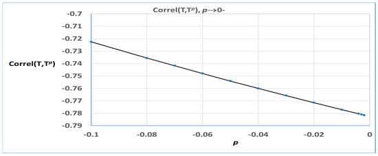
This correlation is illustrated in Table 1 and Figure 1 for ~ E() and values of p on and between −0.1 and −0.001. The correlations are averages calculated from 1000 samples of 500 numbers each, obtained from Matlab [31]. The correlation between and is seen to be negative, approaching −0.7821.
Unlike the case of the lognormal distribution, where the limiting correlation between the random variable and its infinitesimal negative pth exponent is −1, here, the limiting correlation is ≈−0.78. That is, and can only offer partial antithetic combining. In order to convert back into the units of , consider the regression of on , If the correlation were −1, that is, and were perfectly negatively correlated, it would follow that Since the correlation is ≈−0.78, we will use the approximation . Let the fitted values of be denoted by , let and denote the least square estimates of and , respectively, and let s denote the standard deviation. Then, as p0−. This random variable is negatively correlated with This fitted regression equation can be used to convert back to the original scale of
3. Computer Simulation Experiment
The computer simulation in our experiment is depicted in Figure 2. The schematic shows the various queueing systems to be analyzed by Monte Carlo experiments. An example of a queueing system is jobs waiting to be processed by a computer’s central processing unit (CPU). There are many examples. This particular system is an M/M/1 queueing system. The time between arrivals is an exponentially distributed random variate. The mean arrival rate is . The mean time between arrivals is 1/. The service time is an exponentially distributed random variate. The service rate is μ. The mean service time is 1/μ. In this simple queue, the source population for arriving entities is infinite. The queue is un-capacitated. There is a single server. The entity processing rule is first come first served. This is a test system in which the time in the system can be determined exactly from queueing theory. For these parameters, the time in the system is 1/(1/μ − 1/λ) For convenience, in Section 2 will now be replaced by T, where it is understood that T represents a time series.
In the standard traditional experiment, the experiment is conducted with an inter-arrival time denoted by derived from the uniformly distributed random number and service time derived from the uniformly distributed random number . The LCG (suggested by Harrell, Ghosh, and Bowden [32]) is = 630,360,016mod(). It is deployed in their Promodel commercial software package, which is widely used by engineers and managers.
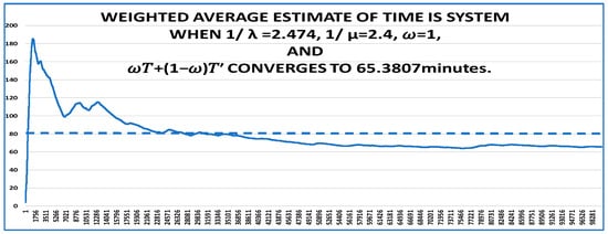
The first simulation scenario is based on a mean inter-arrival time of 3 min and a mean service rate of 2.4 min. That is, λ = 1/3 per minute and μ = 1/2.4 per minute. The response variable chosen is the average time that an entity spends in the system. The average time that entities spend in the system is well known to be precisely = 1/(μ − λ) = 1/(1/2.4 − 1/3) = 12 min. Based on a 100,000 arrivals simulation, the estimated simulation time in the system is T = 11.63 (see Table 2). The bias is 12 − 11.65 = 0.35 = 2.92%. For most applications this level of accuracy may suffice. However, as the λ/μ ratio increases toward 1, the bias increases, and the decline in accuracy is significant. Table 2 shows the results for various λ/μ ratios. For an example of high bias, consider μ = 1/2.4, 1/λ = 2.474, λ/μ = 0.97, the = 1/(1/2.4–1/2.474) = 80.24 min. The estimated simulation time in the system is T = 65.3807 (see Figure 3). The bias = 65.3807–80.24 = −14.8593 = −18.51%. This bias is unacceptable, as are many estimates in Table 2. If any one of these λ/μ values produce errors in the time in the system, it illustrates the problem that we said can occur in the simulation. The systematic change in the bias error with λ/μ illustrates that the occurrence is not accidental. These results also provide a general understanding of antithetic power transformation and insights into how unbiased simulation systems might be implemented.
To reduce this bias, the antithetic time in the system is obtained from where p = −0.0001. Then, T is regressed on to express in the original units of T. The estimated regression equation is given by
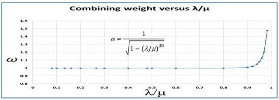
The final result is the weighted average , where and are combining weights. For each combination of μ and λ, there is an for the corresponding λ/μ ratio that results in negligible bias (estimated in bold numbers).
4. Optimizing the Combining Weights
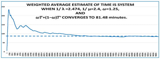
A graph of for various λ/μ ratios that result in negligible bias (estimated in bold numbers) is given in Figure 4. This graph of is a smooth monotonically increasing function of λ/μ. The optimization of the weight is performed by consulting Figure 4 once the λ/μ ratio for the system design is known. Further analysis of the data for Figure 4 reveals the functional relationship between and A graph of simulation estimates of time in the system when 1/λ = 2.474, 1/μ = 2.4 min, = 1.25, and converges to 81.48 min is given is Figure 5. The graph is created once is obtained from Figure 4. The bias is now 80.24 − 81.48 = 1.24 = 1.5%. This is acceptable. We also observe that the shapes of the graphs in Figure 3 and Figure 5 are essentially the same, except that one is biased and one is unbiased.
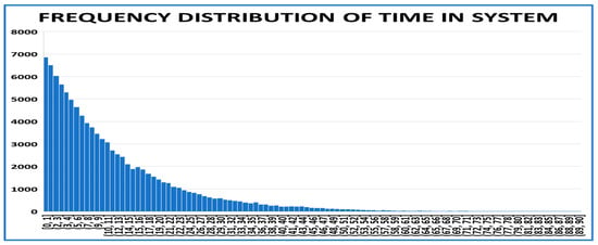
The next analysis will focus on the correlation structure associated with the response variable (T). First, we examine the distribution of the response variable. A histogram of the response variable is shown in Figure 6. The distribution is similar in appearance to an exponential distribution. From Section 2, the correlation between an exponential variate and its power transformation is ≈−0.78. So, one might expect Correl(T, ) as p → 0− to be in the neighborhood of −0.78. We are interested in the relationship between and Correl(T, ), with the idea of using Correl(T, ) as an estimator of . It turns out, for this simulation, that as p → 0−, Correl(T, ) ≈ −0.8 and Correl(T, ) ≈ −0.8. The effect of correlation in the random numbers is embedded in this empirical correlation structure of the response variable. We can think of the mean time in the system as the parameter of its exponential probability distribution.
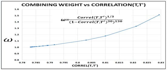
Analysis of the data for T and reveals the graph shown in Figure 7. This graph is a smooth monotonically increasing function of Correl(T,). It permits the optimization of without having to know the λ/μ ratio. Optimization of the weight is performed by consulting the graph once Correl (T, ) for the system design is calculated from T and . Further analysis of the data for Figure 7 reveals the functional relationship between ω and
5. Conclusions
The Monte Carlo experiments reported in this paper are for a simple queue for which the system response variable and time in the system are known from theory. That way we can determine if the simulation estimate is accurate. The simulations demonstrate the presence of hidden errors in the response variable. It is assumed that this bias is due to traces of serial correlation in the random numbers on which the simulation was based. If the bias is due to pre-simulation traces of serial correlation, then since subsets of correlation are part of the overall randomness, bias cannot be avoided by better random numbers. This appears to be an artifact of the Monte Carlo simulation that cannot be improved by the choice of random numbers. It is unlikely that better random numbers will make this problem go away. It appears that the serially correlated random numbers produce a response variable time series in which serial correlation becomes embedded in the correlation structure of time in the system.
To correct the problem, antithetic random variables were created from the response variable and its power transformation. These formed antithetic variables that were combined. The combining weights were determined to be a function of correlation between the response variable and its antithetic counterpart. The combined variable was proven to contain negligible bias. The combined estimates were closer to their corresponding values that are known to be true from theory, combining reduced bias in the estimated values.
Future research might be conducted for different system designs and antithetic variable combining strategies. The Ferrenberg, Lanau, and Wong [6] lattice gauge problem can be revisited by applying the method discussed here. One might also investigate the possibility of deriving the function for the antithetic combining weight from a study of the topology that describes the relationship between the weight and the correlation structure of the system response variable with its antithetic counterpart.
Author Contributions
D.R.: Conceptualization, topic selection, experiment design, methodology, computations, writing, supervision. D.R. and P.N.: Mathematical proofs. All authors have read and agreed to the published version of the manuscript.
Funding
This research received no external funding.
Data Availability Statement
All data are generated in the paper.
Conflicts of Interest
The authors declare no conflict of interest.
Appendix A. Correlation between and
Consider the random variable that has exponential distribution with mean Its pdf is given by
Its moment-generating function is . A quick evaluation of the resulting improper integral yields
Let be a positive integer, then the derivative of is
It is well known that , for a positive integer greater or equal to 1.
in Equation (A2) contains factorial for positive integers. The Gamma function see (Andrews, Askey, and Roy [33]) is also known as the generalized factorial. Euler’s second integral can be extended to include all real valued arguments excluding the negative values as follows:
Expression (A3) will be used to extend Expression (A2) for non-positive integer values as follows:
Equation (A4) can be extended to complex values p such that .
It follows from (A4) that:
The Maclaren series expansions of the terms in Equation (A5) are
where is the Euler-Mascheroni constant defined by
We then obtain
Similarly,
Therefore, ; and and
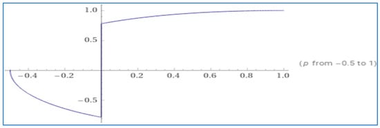
This limiting correlation is in a δ neighborhood of 0. There is a discontinuity at 0. See Figure A1.
References
- Lehmer, D.H. Mathematical methods in large-scale computing units. Annu. Comput. Lab. Harvard Univ. 1951, 26, 141–146. [Google Scholar]
- Devroye, L. Nonuniform Variate Generation; Springer: Berlin/Heidelberg, Germany; New York, NY, USA, 1986. [Google Scholar]
- Franklin, J.N. Deterministic simulation of random processes. Math. Comput. 1963, 17, 28–59. [Google Scholar] [CrossRef]
- Ermakov, S.M. Note on pseudorandom sequences. USSR Comput. Math. Math. Phys. 1972, 12, 307–314. [Google Scholar] [CrossRef]
- Proykova, A. How to improve a random number generator. Comput. Phys. Commun. 2000, 124, 125–131. [Google Scholar] [CrossRef]
- Ferrenberg, A.M.; Landau, D.P.; Wong, J.Y. Monte Carlo Simulations: Hidden errors from “good” random number generators. Phys. Rev. Lett. 1992, 69, 3382–3384. [Google Scholar] [CrossRef]
- Peterson, I. The Bias of Random-Number Generators; MathTrek: Milpitas, CA, USA, 2003. [Google Scholar]
- Marsaglia, G. Random numbers fall mainly in the planes. Proc. Natl. Acad. Sci. USA 1968, 61, 25–28. [Google Scholar] [CrossRef] [PubMed]
- Park, S.K.; Miller, K.W. Random Number Generators: Good Ones Are Hard To Find. Commun. ACM 1988, 31, 1192–1201. [Google Scholar] [CrossRef]
- Marsaglia, G. Expressing a random variable in terms of uniform random variables. Ann. Math. Stat. 1961, 32, 894–898. [Google Scholar] [CrossRef]
- Marsaglia, G. Generating a variable from the tail of the normal distribution. Technometrics 1964, 6, 101–102. [Google Scholar]
- Marsaglia, G.; Tsang, W.W. The Monte Python method for generating random variable. ACM Trans. Math. Softw. 1988, 24, 341–350. [Google Scholar] [CrossRef]
- Marsaglia, G.; Tsay, L.H. Matrices and the structure of random number sequences. Linear Algebra Its Appl. 1985, 67, 147–156. [Google Scholar] [CrossRef]
- Marsaglia, G.; MacLaren, M.D.; Bray, T.A. A fast procedure for generating normal random variables. Commun. ACM 1964, 7, 3–10. [Google Scholar]
- Marsaglia, G.; MacLaren, M.D. A fast procedure for generating exponential random variables. Commun. ACM 1964, 7, 298–300. [Google Scholar] [CrossRef]
- Marsaglia, G.; Ananthanarayan, K.; Paul, N.J. Improvements on fast methods for generating normal random variables. Inf. Process. Lett. 1976, 5, 27–30. [Google Scholar] [CrossRef]
- Marsaglia, G.; Tsang, W.W. A fast, easily implemented method for sampling from decreasing or symmetric unimodal density functions. SIAM J. Sci. Stat. Comput. 1984, 5, 349–359. [Google Scholar] [CrossRef]
- Leva, J.L. A fast normal random number generator. ACM Trans. Math. Sofware 1992, 18, 454–455. [Google Scholar] [CrossRef]
- Kroese, D.P.; Taimre, T.; Botev, Z.I. Handbook of Monte Carlo Methods; John Wiley & Sons: New York, NY, USA, 2011. [Google Scholar]
- Hammersley, J.M.; Morton, K.W. A new Monte Carlo technique: Antithetic variates. Math. Proc. Camb. Philos. Soc. 1956, 52, 449–475. [Google Scholar] [CrossRef]
- Cheng, R.C.H. The Use of Antithetic Variates in Computer Simulations. J. Opl. Res. Soc. 1982, 33, 229–237. [Google Scholar] [CrossRef]
- Kleijnen, J.P.C. Antithetic variates, common random numbers and optimal computer time allocation in simulation. Manag. Sci. 1975, 21, 1176–1185. [Google Scholar] [CrossRef]
- Garcia-Pareja, S.; Lallena, A.M.; Salvat, F. Variance-Reduction Methods for Monte Carlo Simulation of Radiation Transport. Front. Phys. 2021, 2021, 633. [Google Scholar] [CrossRef]
- Ridley, A.D. Optimal Antithetic Weights for Lognormal Time Series Forecasting. Comput. Oper. Res. 1999, 26, 189–209. [Google Scholar] [CrossRef]
- Ridley, A.D. Combining Global Antithetic Forecasts. Int. Trans. Oper. Res. 1995, 2, 387–398. [Google Scholar] [CrossRef]
- Ridley, A.D. Optimal Weights for Combining Antithetic Forecasts. Comput. Ind. Eng. 1997, 32, 371–381. [Google Scholar] [CrossRef]
- Ridley, A.D.; Ngnepieba, P.; Duke, D. Parameter Optimization for Combining Lognormal Antithetic Time Series. Eur. J. Math. Sci. 2013, 2, 235–245. [Google Scholar]
- Ridley, A.D.; Ngnepieba, P. Antithetic time series analysis and the CompanyX data. J. R. Stat. Soc. A 2014, 177, 83–94. [Google Scholar] [CrossRef]
- Ridley, A.D.; Ngnepieba, P. General Theory of Antithetic Time Series. J. Appl. Math. Phys. 2015, 3, 1726–1741. [Google Scholar]
- Ridley, A.D. Advances in Antithetic Time Series: Separating fact from artifact. Oper. Res. Decis. 2016, 26, 57–68. [Google Scholar] [CrossRef]
- MATLAB. Application Program Interface Reference, Version 8; The MathWorks, Inc.: Natick, MA, USA, 2008. [Google Scholar]
- Harrell, C.; Ghosh, B.; Bowden, R. Simulation Using Promodel; McGraw Hill: New York, NY, USA, 2004. [Google Scholar]
- Andrews, G.E.; Askey, R.; Roy, R. Special Functions; Cambridge University Press: Cambridge, UK, 1999. [Google Scholar]
Disclaimer/Publisher’s Note: The statements, opinions and data contained in all publications are solely those of the individual author(s) and contributor(s) and not of MDPI and/or the editor(s). MDPI and/or the editor(s) disclaim responsibility for any injury to people or property resulting from any ideas, methods, instructions or products referred to in the content. |
© 2023 by the authors. Licensee MDPI, Basel, Switzerland. This article is an open access article distributed under the terms and conditions of the Creative Commons Attribution (CC BY) license (https://creativecommons.org/licenses/by/4.0/).

