New Spectral Results for Laplacian Harary Matrix and the Harary Laplacian-Energy-like Applying a Matrix Order Reduction

Abstract

In this paper, we introduce the concepts of Harary Laplacian-energy-like for a simple undirected and connected graph G with order n. We also establish novel matrix results in this regard. Furthermore, by employing matrix order reduction techniques, we derive upper and lower bounds utilizing existing graph invariants and vertex connectivity. Finally, we characterize the graphs that achieve the aforementioned bounds by considering the generalized join operation of graphs.

1. Introduction and Preliminaries

Throughout the paper, let $G=(V,E)$ be a connected simple undirected graph with vertex set V and edge set E. The order of a graph is the cardinality of its vertex set, $\left|V\right|$, the size of a graph is the cardinality of its edge set, $\left|E\right|$, and $A\left(G\right)$ is the adjacency matrix associated with the graph G of order n with eigenvalues ${\lambda }_i\left(A\left(G\right)\right),$ for all $i=1,\dots ,n.$

The energy of a graph is a concept that comes from theoretical chemistry and is studied in mathematical chemistry to approximate the total $\pi$-electron energy of a molecule [1,2,3]. In 1978, Ivan Gutman defined the energy of a graph through the eigenvalues of the adjacency matrix of a graph [4] as

$$E\left(G\right)=\sum _{i=1}^n\left|{\lambda }_i\left(A\left(G\right)\right)\right|.$$

It should be noted that the interest for this graph invariant goes far beyond chemistry; for example, it is used for minimum and maximum energy for certain families of graphs [5,6,7], on upper and lower bounds for the energy of graphs [8,9,10,11], and the extension of energy to the Laplacian energy of graphs [12]. Additionally, in [13], the authors list various papers published in 2019 on graph energies, and summarize their main collective characteristics, but an interesting motivation is that the authors cite articles that show applications of graph energy outside the field of mathematics. For example, in [14], a topic related to climate change is addressed; the authors identify the vertices of a graph with the terms “soil”, “climate”, “hydrogeomorphic features”, “biotic features”, and similar, connected by directed or undirected edges, and, in this case, the respective energy “indicates the overall strength of positive and negative feedbacks present”.

In 2008, Liu and Liu defined the Laplacian-energy-like of a graph [15] as

$$LEL\left(G\right)=\sum _{i=1}^n\sqrt{{\mu }_i}$$

where ${\mu }_1\left(G\right)\ge {\mu }_2\left(G\right)\ge \dots \ge {\mu }_n\left(G\right)=0$ are the Laplacian eigenvalues of G.

The authors in [15] have shown that this invariant has similar features to molecular graph energy, see [4]. In [16], it was demonstrated that $LEL$ can be used both in graph discriminating analysis and in correlating studies for modeling a variety of physical and chemical properties and biological activities. This motivates us to extend the results of $LEL$ by considering other matrices associated with graphs that can be representations of various physical or chemical phenomena.

The distance between the vertices $v_i$ and $v_j$ of G, denoted by $d\left(v_i,v_j\right)=d_{i,j}$, is equal to the length of (number of edges in) the shortest path that connects $v_i$ and $v_j$. The Harary matrix of graph G, which is also called the reciprocal distance matrix, and is denoted by $RD\left(G\right)$, was defined in 1993, independently in [17,18], as a matrix of order n, given by

$$RD{\left(G\right)}_{i,j}=\left\{\begin{array}{cc}\frac{1}{d\left(v_i,v_j\right)}& \mathrm{if}i\ne j\\ 0& \mathrm{if}i=j.\end{array}\right.$$

Henceforth, we consider $i\ne j$ for $d\left(v_i,v_j\right)$.

The reciprocal distance degree of a vertex v, denoted by $RT\left(v\right)$, is given by

$$RT\left(v\right)=\sum _{\underset{u\ne v}{u\in V\left(G\right)}}\frac{1}{d\left(u,v\right)}.$$

Let $RT\left(G\right)$ be the diagonal Harary degree matrix of order n defined by $R{T}_{i,i}=R{T}_i=RT\left(v_i\right)$ for $i=1,\dots ,n$.

The Harary index of a graph G, denoted by $H\left(G\right)$, is defined in [17,18] as

$$H\left(G\right)=\frac{1}{2}\sum _{i=1}^n\sum _{j=1}^{n}RD{\left(G\right)}_{i,j}=\frac{1}{2}\sum _{\underset{u\ne v}{u,v\in V\left(G\right)}}\frac{1}{d\left(u,v\right)}.$$

Clearly,

$$H\left(G\right)=\frac{1}{2}\sum _{v\in V\left(G\right)}RT\left(v\right).$$

In 2018, the authors defined the reciprocal distance Laplacian matrix [19] as

$$RL\left(G\right)=RT\left(G\right)-RD\left(G\right).$$

Since $RL\left(G\right)$ is a real symmetric matrix, we can write its eigenvalues in decreasing order

$${\lambda }_1\left(RL\left(G\right)\right)\ge {\lambda }_2\left(RL\left(G\right)\right)\ge \dots \ge {\lambda }_{n-1}\left(RL\left(G\right)\right)\ge {\lambda }_n\left(RL\left(G\right)\right).$$

We observe that $RL\left(G\right)$ is a positive semi-definite matrix. The following result is fundamental in matrix theory, and will help us to show that the smallest eigenvalue of $RL\left(G\right)$ is simple, i.e., their algebraic multiplicity is one.

Theorem 1

([3] Eigenvalue Interlacing Theorem). Let A be the symmetric matrix of order n. Let B be a principal sub-matrix of order m, obtained by deleting both i-th row and i-th column of A, for some values of i. Suppose A has eigenvalues ${\lambda }_1\ge {\lambda }_2\ge \dots \ge {\lambda }_n$ and B has eigenvalues ${\beta }_1\ge {\beta }_2\ge \dots \ge {\beta }_m$. Then

$${\lambda }_{n-m+k}\le {\beta }_k\le {\lambda }_k,$$

for $k=1,2,\dots ,m$.

A fundamental spectral result of the Laplacian matrix associated with a graph is that its smallest eigenvalue is zero. The following result shows that for the extension $RL\left(G\right)$, zero is also an eigenvalue.

Lemma 1.

Let G be a connected graph on n vertices and let $\mathbf{e}$ be the all one vector. Then, $(0,\mathbf{e})$ is an eigenpair of $RL\left(G\right)$ and 0 is a simple eigenvalue.

Proof. 

Clearly, each row sum of $RL\left(G\right)$ is 0. Thus, $(0,\mathbf{e})$ is an eigenpair of $RL\left(G\right)$. Now, we show that 0 has multiplicity equal to 1.

If $n=1$, the result is immediate.

If $n\ge 2$, then let $R{L}_i$ be the $(n-1)\times (n-1)$ matrix obtained from $RL\left(G\right)$ by eliminating the i-th row and column. Using Theorem 1, we have that

$${\lambda }_n\left(RL\left(G\right)\right)\le {\lambda }_{n-1}\left(R{L}_i\right)\le {\lambda }_{n-1}\left(RL\left(G\right)\right).$$

On the other hand, by construction, we can see that the matrix $R{L}_i$ is strictly diagonal dominant, so $R{L}_i$ is a positive definite matrix. Therefore, ${\lambda }_{n-1}\left(RL\left(G\right)\right)>0$. □

In [20], the authors established bounds for the spectral radius of reciprocal distance Laplacian matrix, and in [21] gave bounds on the reciprocal distance Laplacian energy and characterized the graphs that attained some of those bounds.

Since $RL\left(G\right)$ is a positive semi-definite matrix, then the spectral radius $\rho \left(RL\left(G\right)\right)={\lambda }_1\left(RL\left(G\right)\right)$.

We recall that the notation ${\lambda }^{\left[p\right]}$ means that the eigenvalue $\lambda$ has an algebraic multiplicity equal to p.

Remark 1.

We can see that for the complete graph $K_n,$ $RL\left(K_n\right)=(n-1)I_n-(J_n-I_n)$, where $J_n$ is a matrix with all its entries equal to one and $I_n$ denotes the identity matrix of order n. Then, the $RL\left(K_n\right)$-spectrum is $\{0,n^{[n-1]}\}$.

Theorem 2

([19]). If G is aconnected graph on $n>2$ vertices, then the multiplicity of $\rho \left(RL\left(G\right)\right)$ is $p\le n-1$ with equality if and only if G is the complete graph.

Theorem 3

([19]). Let G be a connected graph on n vertices and $m\ge n$ edges. Consider the connected graph $\tilde{G}$ obtained from G by the deletion of an edge. Let

$${\lambda }_1\left(RL\left(G\right)\right),{\lambda }_2\left(RL\left(G\right)\right),\dots ,{\lambda }_n\left(RL\left(G\right)\right)$$

and

$${\lambda }_1\left(RL\left(\tilde{G}\right)\right),{\lambda }_2\left(RL\left(\tilde{G}\right)\right),\dots ,{\lambda }_n\left(RL\left(\tilde{G}\right)\right)$$

be the reciprocal distance Laplacian spectra of G and $\tilde{G}$, respectively. Then, for all $i=1,\dots ,n$,

$${\lambda }_i\left(RL\left(\tilde{G}\right)\right)\le {\lambda }_i\left(RL\left(G\right)\right).$$

An immediate consequence of Theorem 3 is the following result.

Corollary 1.

Let G be a connected graph on n vertices. Then

$$\rho \left(RL\right(G\left)\right)\le n.$$

At least to the authors’ knowledge, there are several upper bounds, but we only found one lower bound, which is the below theorem

Theorem 4

([20]). Let G be a connected graph on $n\ge 4$ vertices. Then

$$\rho \left(RL\right(G\left)\right)\ge 2H\left(G\right)-n(n-2).$$

Clearly, when n increases, the bound is not adjusted, so in this work we will propose a more appropriate bound. For this, it is necessary to remember the definition of the Frobenius norm of a matrix.

The Frobenius norm of an $n\times n$ matrix $M=\left(m_{i,j}\right)$ is

$${\left|\right|M\left|\right|}_F=\sqrt{\sum _{i=1}^n\sum _{j=1}^n{\left|m_{i,j}\right|}^2}.$$

In particular,

$${\left|\right|RL\left(G\right)\left|\right|}_F^2=\sum _{i=1}^n({\lambda }_i{\left(RL\left(G\right)\right)}^2.$$

Finally, we give the definition of the equitable quotient matrix and its respective spectral result, which will be a fundamental tool in the development of this work.

Definition 1

([22]). Let X be a complex matrix of order n described in the following block form

$$X=\left[\begin{array}{cccc}{X}_{1,1}& X_{1,2}& \dots & X_{1,r}\\ X_{2,1}& X_{2,2}& \dots & X_{2,r}\\ ⋮& ⋮& \ddots & ⋮\\ X_{r,1}& X_{r,2}& \dots & X_{r,r}\end{array}\right]$$

where the blocks $X_{i,j}$ are $n_i\times n_j$ matrices for any $1\le i,j\le r$ and $n=n_1+n_2+\dots +n_r$. For $1\le i,j\le r$, let $b_{i,j}$ denote the average row sum of $X_{i,j}$, i.e., $b_{i,j}$ is the sum of all entries in $X_{i,j}$ divided by the number of rows. Then $B\left(X\right)=\left(b_{i,j}\right)$ is called the quotient matrix of X. If for each pair $i,j$, $X_{i,j}$ has a constant row sum, then $B\left(X\right)$ is called the equitable quotient matrix of X.

Theorem 5

([23]). Let $B\left(X\right)$ be the equitable quotient matrix of X as defined in Definition 1. Then, the spectrum of $B\left(X\right)$ is contained in the spectrum of X.

In this paper, applying the block division matrix technique and using the quotient matrix, new spectral results are obtained from the reciprocal Laplacian matrix. Additionally, we obtain the eigenvalues of certain graphs and in particular obtain eigenvalues of the generalized join product of regular graphs. Finally, we apply these results to obtain extreme graphs, among all the connected graphs of prescribed order in terms of the vertex connectivity, for the energy that we define as Harary Laplacian-like energy, denoted by $HLEL\left(G\right)$ as

$$HLEL\left(G\right)=\sum _{i=1}^{n-1}\sqrt{{\lambda }_i\left(RL\left(G\right)\right)}.$$

2. Main Spectral Results

In this section, we give some spectral results about the $RL\left(G\right)$ matrix. In particular, we give a new lower bound for the spectral radius and we characterize the spectrum of certain types of graphs. Our result is more appropriate than the one given by Theorem 4, since for any value of n it is positive and we also characterize when this bound is obtained.

Theorem 6.

Let G be a connected graph on $n\ge 2$ vertices. Then

$$\rho \left(RL\left(G\right)\right)\ge \frac{{\left|\right|RL\left(G\right)\left|\right|}_F^2}{2H\left(G\right)}.$$

The equality holds if and only if $G=K_n$.

Proof. 

Since G is a connected graph of order $n\ge 2$, then, from Lemma 1, for $i=1,\dots ,n-1$

$${\lambda }_i\left(RL\left(G\right)\right)>0$$

and

$$\rho \left(RL\left(G\right)\right){\lambda }_i\left(RL\left(G\right)\right)\ge {\left({\lambda }_i\left(RL\left(G\right)\right)\right)}^2.$$

Thus

$$\rho \left(RL\left(G\right)\right)\left(\sum _{i=1}^{n-1}{\lambda }_i\left(RL\left(G\right)\right)\right)\ge {\lambda }_1{\left(RL\left(G\right)\right)}^2+\dots +{\lambda }_{n-1}{\left(RL\left(G\right)\right)}^2.$$

(1)

Therefore

$$\rho \left(RL\left(G\right)\right)\ge \frac{{\left|\right|RL\left(G\right)\left|\right|}_F^2}{2H\left(G\right)}.$$

The equality holds if and only if the equality (1) holds, and this is

$$\rho \left(RL\left(G\right)\right)={\lambda }_2\left(RL\left(G\right)\right)=\dots ={\lambda }_{n-1}\left(RL\left(G\right)\right).$$

Therefore, the multiplicity of $\rho \left(RL\right(G\left)\right)$ is $n-1$. Using Theorem 2, we conclude that $G=K_n$. □

A pair of vertices u and v in G are called twins if they have the same neighborhood, and the same edge weights in the case of a weighted graph. Twin vertices in graphs have proven very useful in the study of the spectra. Motivated by the study of eigenvalues of the adjacency and Laplacian matrices when there are twin vertices in a graph, we study the eigenvalues for the matrix $RL\left(G\right)$.

If $uv$ is an edge in G, they are called adjacent twins, and if $uv$ is not an edge in G, they are called non-adjacent twins.

Theorem 7.

Let G be a connected graph of order n and U be a subset of $V\left(G\right)$ such that U is a set of non-adjacent twins, with $\left|U\right|=t$. Then $RT\left(v\right)=h$ is constant for each $v\in U$ and $\left(h+\frac{1}{2}\right)$ is an eigenvalue of $RL\left(G\right)$ with a multiplicity of at least $t-1$.

Proof. 

Without loss of generality, we can label the vertices of U as $v_1,\dots ,v_t$. Then $d\left(v_i,v_k\right)=d\left(v_j,v_k\right)$ for all $v_i,v_j\in U$ and for all $v_k\in V\left(G\right)$, in particular $d\left(v_i,v_j\right)=2$ for all $v_i,v_j\in U$. We note that $RT\left(v_i\right)=RT\left(v_j\right)$ for all $v_i,v_j\in U$. Let $h=RT\left(v_i\right)$ for all $v_i\in U$ and let $X_i={\mathbf{e}}_1-{\mathbf{e}}_{i+1}$ for $i=1,2,\dots ,t-1$ where ${\mathbf{e}}_i$ is the i-th canonical vector. Then

$$RL\left(G\right)X_i={\left[h+\frac{1}{2},0,\dots ,0,-\frac{1}{2}-h,0,\dots ,0\right]}^T=\left(h+\frac{1}{2}\right)X_i.$$

Since $X_1,X_2,\dots ,X_{t-1}$ are linearly independent, $\left(h+\frac{1}{2}\right)$ is an eigenvalue of $RL\left(G\right)$ with a multiplicity of at least $t-1$. □

Proposition 1.

Let ${\mathcal{T}}_{a,b}$ be a tree of diameter 3 and order $n=a+b+2\ge 4$. Then the $RL$-eigenvalues are $\left\{{\left(\frac{3a+2b+9}{6}\right)}^{[a-1]},{\left(\frac{2a+3b+9}{6}\right)}^{[b-1]}\right\}$ and the eigenvalues of the matrix

$$\left[\begin{array}{cccc}\frac{2b+9}{6}& -1& -\frac{1}{2}& -\frac{b}{3}\\ -a& \frac{2a+b+2}{2}& -1& -\frac{b}{2}\\ -\frac{a}{2}& -1& -\frac{a+2b+2}{2}& b\\ -\frac{a}{3}& -\frac{1}{2}& -1& \frac{2a+9}{6}\end{array}\right].$$

Proof. 

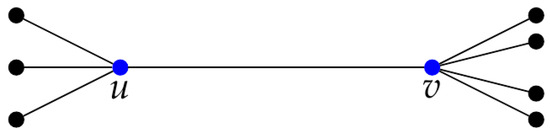
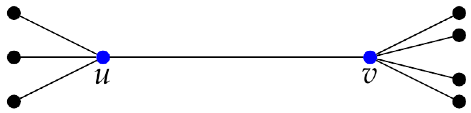
Let u, v be the central vertices of a tree of diameter 3 (see Figure 1). Consider the following partition of the graph ${\mathcal{T}}_{a,b}$

$$\left\{V_1,\left\{u\right\},\left\{v\right\},V_2\right\}.$$

Figure 1. A tree ${\mathcal{T}}_{3,4}$ of diameter 3 and order $n=9$ is shown in the above image.

Clearly, $V_1$ and $V_2$ are independent sets to ${\mathcal{T}}_{a,b}$ such that for any $x,y\in V_1$, $N\left(x\right)=N\left(y\right)=u$ and for any $x,y\in V_2$, $N\left(x\right)=N\left(y\right)=v,$ where $N\left(v\right)$ denotes the neighboring vertices of $v\in V\left(G\right).$

We observe that for all vertex $v_i$ in $V_1$ we have $R{T}_i=\frac{a-1}{2}+1+\frac{1}{2}+\frac{b}{3}=\frac{3a+2b+6}{6}$, analogously for all vertex $v_j$ in $V_2$, and $R{T}_j=\frac{2a+3b+6}{6}$. Then, using Theorem 7, we have that $\frac{3a+2b+9}{6}$ and $\frac{2a+3b+9}{6}$ are eigenvalues of $RL\left({\mathcal{T}}_{a,b}\right)$ with multiplicities $a-1$ and $b-1$, respectively.

Let $R{T}_a=\frac{3a+2b+6}{6}$ and $R{T}_b=\frac{2a+3b+6}{6}$. Then, $RL\left({\mathcal{T}}_{a,b}\right)$ has the following block matrix form

$$RL\left({\mathcal{T}}_{a,b}\right)=\left[\begin{array}{cccc}R{T}_{a}I-\frac{1}{2}[J_a-I_a]& -\left[J_{a\times 1}\right]& -\frac{1}{2}\left[J_{a\times 1}\right]& -\frac{1}{3}\left[J_{a\times b}\right]\\ -\left[J_{1\times a}\right]& \frac{2a+b+2}{2}& -1& -\frac{1}{2}\left[J_{1\times b}\right]\\ -\frac{1}{2}\left[J_{1\times a}\right]& -1& \frac{a+2b+2}{2}& -\left[J_{1\times b}\right]\\ -\frac{1}{3}\left[J_{b\times a}\right]& -\frac{1}{2}-\left[J_{b\times 1}\right]& \left[J_{b\times 1}\right]& R{T}_{b}I-\frac{1}{2}[J_b-I_b]\end{array}\right].$$

Let $M\left({\mathcal{T}}_{a,b}\right)$ be the equitable quotient matrix of $RL\left({\mathcal{T}}_{a,b}\right),$ considering that each block has a constant row sum, an then we can write

$$M\left({\mathcal{T}}_{a,b}\right)=\left[\begin{array}{cccc}R{T}_a-\frac{a-1}{2}& -1& -\frac{1}{2}& -\frac{b}{3}\\ -a& R{T}_u& -1& -\frac{b}{2}\\ -\frac{a}{2}& -1& R{T}_v& -b\\ -\frac{a}{3}& -\frac{1}{2}& -1& R{T}_b-\frac{b-1}{2}\end{array}\right].$$

Applying Theorem 5, the eigenvalues of $M\left({\mathcal{T}}_{a,b}\right)$ are eigenvalues of $RL\left({\mathcal{T}}_{a,b}\right)$. Finally, replacing $R{T}_a=\frac{3a+2b+6}{6}$, $R{T}_b=\frac{2a+3b+6}{6}$, $R{T}_u=\frac{2a+b+2}{2}$ and $R{T}_v=\frac{a+2b+2}{2}$, the matrix given in Theorem is obtained. □

A set of vertices that induces a subgraph with no edges is called an independent set. A bipartite graph is a graph whose vertex set can be partitioned into two disjoint and independent sets $V_1$ and $V_2$, that is, every edge connects a vertex in $V_1$ to one in $V_2$. A complete bipartite graph is a special kind of bipartite graph where every vertex of the first set is adjacent to every vertex of the second set. A complete bipartite graph with partitions of size $|V_1|=a$ and $|V_2|=b$ is denoted by $K_{a,b}$. A star graph is a complete bipartite graph with partitions of size $|V_1|=1$ and $|V_2|=n-1$. The star graph of order n is denoted either by $K_{1,n-1}$ or $S_n$.

The following proposition gives us the eigenvalues of a complete bipartite graph associated to the reciprocal distance Laplacian matrix.

Proposition 2.

Let $K_{a,b}$ be a complete bipartite graph on $n=a+b$ vertices. Then, the spectrum of $RL\left(K_{a,b}\right)$ is

$$\begin{array}{cc}\hfill \sigma \left(RL\left(K_{a,b}\right)\right)=& \left\{n,{\left(\frac{a+2b}{2}\right)}^{\left[a-1\right]},{\left(\frac{2a+b}{2}\right)}^{\left[b-1\right]},0\right\}.\end{array}$$

Proof. 

Since $V_1$ and $V_2$ are independent sets to $K_{a,b}$ such that for any $x,y\in V_1$, $N\left(x\right)=N\left(y\right)=V_2$ and for any $x,y\in V_2$, $N\left(x\right)=N\left(y\right)=V_1$, then for all $v_i\in V_1$, we obtain that $R{T}_i=\frac{a+2b-1}{2}$ and for all vertex $v_j\in V_2$ we have that $R{T}_j=\frac{2a+b-1}{2}$. Now, using Theorem 7, we have that $\frac{a+2b}{2}$ is an eigenvalue with multiplicity $a-1$ and $\frac{2a+b}{2}$ is an eigenvalue with multiplicity $b-1$.

From Lemma 1, we have that zero is always an eigenvalue of the matrix $RL\left(G\right)$. We observe that $\frac{a+2b}{2}$ and $\frac{2a+b}{2}$ are non-zero. Therefore, we have $n-1$ eigenvalues. We obtain the other eigenvalue by applying the fact that the trace of the matrix is equal to the sum of its eigenvalues and the trace of $RL\left(G\right)$ is equal to the sum of its reciprocal distance degrees. □

Corollary 2.

Let $S_n$ be the star graph on $n\ge 3$ vertices. Then the spectrum of the reciprocal distance Laplacian matrix of $S_n$ is

$$\sigma \left(RL\left(S_n\right)\right)=\left\{n,{\left(\frac{n+1}{2}\right)}^{\left[n-2\right]},0\right\}.$$

Theorem 8.

Let G be a connected graph of order n and U be a subset of $V\left(G\right)$ such that U is a set of adjacent twins, with $\left|U\right|=t$. Then, $RT\left(v\right)=h^{\prime }$ is constant for each $v\in U$ and $\left(h^{\prime }+1\right)$ is an eigenvalue of $RL\left(G\right)$ with multiplicity at least $t-1$.

Proof. 

Without loss of generality, we can label the vertices of U as $v_1,\dots ,v_t$. Then $d\left(v_i,v_k\right)=d\left(v_j,v_k\right)$ for all $v_i,v_j\in U$ and for all $v_k\in V\left(G\right)$, and in particular $d\left(v_i,v_j\right)=1$ for all $v_i,v_j\in U$. Thus, $RT\left(v_i\right)=RT\left(v_j\right)$ for all $v_i,v_j\in U$. Let $h^{\prime }=RT\left(v_i\right)$ for all $v_i\in U$ and let $X_i={\mathbf{e}}_1-{\mathbf{e}}_{i+1}$ for $i=1,2,\dots ,t-1$. Then,

$$RL\left(G\right)X_i={\left[h^{\prime }+1,0,\dots ,0,-1-h^{\prime },0,\dots ,0\right]}^T=\left(h^{\prime }+1\right)X_i.$$

Since $X_1,X_2,\dots ,X_{t-1}$ are linearly independent, $\left(h^{\prime }+1\right)$ is an eigenvalue of $RL\left(G\right)$ with a multiplicity of at least $t-1$. □

A clique of a graph is a subset of vertices in which every two vertices are adjacent. A complete split graph, denoted by $C{S}_{a,n-a}$, is a graph consisting of a clique of a vertices and an independent set of the remaining $n-a$ vertices, such that each vertex in the clique is adjacent to every vertex in the independent set.

Proposition 3.

Let $C{S}_{a,n-a}$ be a complete split graph on n vertices. Then

$$\sigma \left(RL\left(C{S}_{a,n-a}\right)\right)=\left\{n^{\left[a\right]};{\left(\frac{n+a}{2}\right)}^{\left[n-a-1\right]};0\right\}.$$

Proof. 

Notice that for the clique of order a, we have that

$$h^{\prime }=1\left(a-1\right)+1\left(n-a\right)=n-1.$$

Applying Theorem 8, we obtain that n is an $RL$-eigenvalue of $C{S}_{a,n-a}$ with a multiplicity of at least $a-1$.

Analogously, for the independent set of order $n-a$, we have that

$$h=\frac{1}{2}\left(n-a-1\right)+1\left(a\right)=\frac{\left(n+a-1\right)}{2}.$$

Applying Theorem 7, we obtain that

$$\frac{\left(n+a-1\right)}{2}+\frac{1}{2}=\frac{n+a}{2}$$

is an $RL$-eigenvalue of $C{S}_{a,n-a}$ with a multiplicity of at least $n-a-1$.

From Lemma 1, we have that zero is always an eigenvalue of the matrix $RL\left(G\right)$. Since $\frac{n+a}{2}\ne 0$, we have $n-1$ eigenvalues. We obtain the other eigenvalue by applying the fact that the trace of the matrix is equal to the sum of its eigenvalues, and the trace of $RL\left(G\right)$ is equal to the sum of its reciprocal distance degrees. □

Finally, in this section, we study the spectrum for the generalized join graph operation. In particular, we characterize the spectrum of the reciprocal distance Laplacian matrix for the generalized join of regular graphs. We study this operation between graphs since certain graphs can be expressed as a join product of graphs of a much lower order, reducing the process of obtaining their eigenvalues. Furthermore, in the final part of the next section, we use the join product of certain types of graphs to obtain bounds for the Harary Laplacian-energy-like.

Let $G_1=(V_1,E_1)$ and $G_2=(V_2,E_2)$ be two vertex disjoint graphs. The join graph operation of $G_1$ and $G_2$ is the graph $G=G_1\vee G_2$ such that $V\left(G\right)=V\left(G_1\right)\cup V\left(G_2\right)$ and $E\left(G\right)=E\left(G_1\right)\cup E\left(G_2\right)\cup \{xy:x\in V\left(G_1\right),y\in V\left(G_2\right)\}$. This join operation can be generalized as follows [24]: Let $\mathcal{H}$ be a graph of order s. Let $V\left(\mathcal{H}\right)=\{v_1,\dots ,v_s\}$. Let $\{G_1,\dots ,G_s\}$ be a set of pairwise vertex disjoint graphs. For $1\le i\le s$, the vertex $v_i\in V\left(\mathcal{H}\right)$ is assigned to the graph $G_i$. Let G be the graph obtained from the graphs $G_1,\dots ,G_s$ and the edges connecting each vertex of $G_i$ with all the vertices of $G_j$ if and only if $v_i,v_j\in E\left(\mathcal{H}\right)$. That is, G is the graph with vertex set $V\left(G\right)={\bigcup }_{i=1}^{s}V\left(G_i\right)$ and edge set

$$E\left(G\right)=\left(\bigcup _{i=1}^{s}E\left(G_i\right)\right)\bigcup \left(\bigcup _{v_i,v_j\in E\left(\mathcal{H}\right)}\{uv:u\in V\left(G_i\right),v\in V\left(G_j\right)\}\right).$$

This graph operation is denoted by

$$G=\underset{\mathcal{H}}{\bigvee }\{G_i:1\le i\le s\}.$$

Consider the vertices of G with the labels $1,\dots ,{\sum }_{i=1}^s{n}_i$ starting with the vertices of $G_1$, continuing with the vertices of $G_2,G_3,\dots ,G_{s-1}$ and finally with the vertices of $G_s$.

Let $\mathcal{H}$ be a connected graph of order s and for $i=1,\dots ,s$, let $G_i$ be a ${\delta }_i$-degree regular connected graph of order $n_i$. Let $d_{i,j}^{\mathcal{H}}$ be the distance between $v_i,v_j\in V\left(\mathcal{H}\right)$. Here, with the above mentioned labeling, we obtain that the reciprocal distance Laplacian matrix of the $\mathcal{H}$-join $G={\displaystyle \underset{\mathcal{H}}{\bigvee }}\{G_i:1\le i\le s\}$ has the form

$$\begin{array}{ccc}\hfill RL\left(G\right)& =& \left[\begin{array}{cccc}{L}_1& \frac{-1}{d_{1,2}^{\mathcal{H}}}{J}_{n_1\times n_2}& \dots & \frac{-1}{d_{1,s}^{\mathcal{H}}}{J}_{n_1\times n_s}\\ \frac{-1}{d_{1,2}^{\mathcal{H}}}{J}_{n_2\times n_1}& L_2& \ddots & ⋮\\ ⋮& \ddots & \ddots & \frac{-1}{d_{(s-1),s}^{\mathcal{H}}}{J}_{n_{s-1}\times n_s}\\ \frac{-1}{d_{1,s}^{\mathcal{H}}}{J}_{n_s\times n_1}& \dots & \frac{-1}{d_{(s-1),s}^{\mathcal{H}}}{J}_{n_s\times n_{s-1}}& L_s\end{array}\right]\hfill \end{array}$$

(2)

where

$$L_i=k_i{I}_{n_i}+\frac{-1}{2}(J_{n_i}-I_{n_i}+A\left(G_i\right)),$$

(3)

with

$$k_i=\frac{{\delta }_i+n_i-1}{2}+\sum _{j\ne i}\frac{n_j}{d_{i,j}^{\mathcal{H}}}.$$

Notice that the matrices $L_i$ defined in (3) are not necessarily the reciprocal distance Laplacian matrices $L\left(G_i\right)$.

Now, using the results of the partitioned quotient matrix, we will obtain the spectrum of the reciprocal distance Laplacian of the graph $G={\displaystyle \underset{\mathcal{H}}{\bigvee }}\{G_i:1\le i\le s\}$, where $\{G_i,\dots G_s\}$ is a family of a regular graph.

Lemma 2.

Let $L_i$ be the diagonal blocks of the matrix defined in (2) such that, for $i=1,\dots ,s$, $G_i$ is a ${\delta }_i$-regular graph with adjacency eigenvalues $\{{\delta }_i,{\lambda }_2,\dots ,{\lambda }_{n_i}\}$. Then, the spectrum of $L_i$ is

$$\sigma \left(L_i\right)=\left\{\sum _{j\ne i}\frac{n_j}{d_{i,j}^{\mathcal{H}}},k_i+\frac{1}{2}-\frac{1}{2}{\lambda }_{n_i}\left(A\left(G_i\right)\right),\dots ,k_i+\frac{1}{2}-\frac{1}{2}{\lambda }_2\left(A\left(G_i\right)\right)\right\},$$

with $k_i=\frac{{\delta }_i+n_i-1}{2}+\sum _{j\ne i}\frac{n_j}{d_{i,j}^{\mathcal{H}}}$.

Proof. 

Since

$$L_i=k_i{I}_{n_i}+\frac{-1}{2}(J_{n_i}-I_{n_i}+A\left(G_i\right))$$

has constant row sum equal to $k_i-\frac{n_i-1+{\delta }_i}{2}$ where $k_i=\frac{{\delta }_i+n_i-1}{2}+\sum _{j\ne i}\frac{n_j}{d_{i,j}^{\mathcal{H}}}$, and there is l such that

$$L_i{\mathbf{e}}_{n_i}={\lambda }_l\left(L_i\right){\mathbf{e}}_{n_i},$$

with

$${\lambda }_l\left(L_i\right)=\sum _{j\ne i}\frac{n_j}{d_{i,j}^{\mathcal{H}}}.$$

Let $\left\{{\mathbf{e}}_{n_i},{\mathbf{u}}_{i,2},\dots ,{\mathbf{u}}_{i,n_i}\right\}$ be the set of eigenvectors corresponding to the adjacency eigenvalues of regular graph $G_i$, $\{{\delta }_i,{\lambda }_2,\dots ,{\lambda }_{n_i}\},$ respectively. We observe that, for $j=2,\dots ,n_i$, $J_{n_i}{\mathbf{u}}_{i,j}=0{\mathbf{u}}_{i,j}$ and $A\left(G_i\right){\mathbf{u}}_{i,j}={\lambda }_j{\mathbf{u}}_{i,j}$. Then

$$\begin{array}{ccc}\hfill L_i{\mathbf{u}}_{i,j}& =& \left(k_i{I}_{n_i}+\frac{-1}{2}(J_{n_i}-I_{n_i}+A\left(G_i\right))\right){\mathbf{u}}_{i,j}\hfill \\ & =& \left(k_i+\frac{1}{2}-\frac{1}{2}{\lambda }_i\right){\mathbf{u}}_{i,j}.\hfill \end{array}$$

Therefore, for $i=1,\dots ,s$ the spectrum of $L_i$ is

$$\sigma \left(L_i\right)=\left\{\sum _{j\ne i}\frac{n_j}{d_{i,j}^{\mathcal{H}}},k_i+\frac{1}{2}-\frac{1}{2}{\lambda }_{n_i}\left(A\left(G_i\right)\right),\dots ,k_i+\frac{1}{2}-\frac{1}{2}{\lambda }_2\left(A\left(G_i\right)\right)\right\},$$

(4)

with $k_i=\frac{{\delta }_i+n_i-1}{2}+{\displaystyle \sum _{j\ne i}}\frac{n_j}{d_{i,j}^{\mathcal{H}}}$. □

The following result allows us to know the spectrum of new families of regular graphs obtained using the generalized graph join operation.

Theorem 9.

Let $\mathcal{H}$ be a connected graph of order s and $G={\displaystyle \underset{\mathcal{H}}{\bigvee }}\{G_i:1\le i\le s\}$ where, for each $i\in \{1,\dots ,s\}$, $G_i$ is a regular graph. Then, the spectrum of $RL\left(G\right)$ is

$$\sigma \left(RL\left(G\right)\right)=\bigcup _{i=1}^s\left(\sigma \left(L_i\right)\setminus \left\{{\lambda }_l\left(L_i\right)\right\}\right)\cup \sigma \left(F_s\right),$$

where ${\lambda }_l\left(L_i\right)={\displaystyle \sum _{j\ne i}}\frac{n_j}{d_{i,j}^{\mathcal{H}}}$ and $F_s$ is the $s\times s$ matrix

$$F_s=\left[\begin{array}{cccccc}{\lambda }_l\left(L_1\right)& \frac{-1}{d_{1,2}^{\mathcal{H}}}{n}_2& \frac{-1}{d_{1,3}^{\mathcal{H}}}{n}_3& \dots & \frac{-1}{d_{1,(s-1)}^{\mathcal{H}}}{n}_{s-1}& \frac{-1}{d_{1,s}^{\mathcal{H}}}{n}_s\\ \frac{-1}{d_{1,2}^{\mathcal{H}}}{n}_1& {\lambda }_l\left(L_2\right)& \frac{-1}{d_{2,3}^{\mathcal{H}}}{n}_3& \dots & \frac{-1}{d_{2,(s-1)}^{\mathcal{H}}}{n}_{s-1}& \frac{-1}{d_{2,s}^{\mathcal{H}}}{n}_s\\ \frac{-1}{d_{1,3}^{\mathcal{H}}}{n}_1& \frac{-1}{d_{2,3}^{\mathcal{H}}}{n}_2& {\lambda }_l\left(L_3\right)& \dots & \frac{1}{d_{3,(s-1)}^{\mathcal{H}}}{n}_{s-1}& \frac{-1}{d_{3,s}^{\mathcal{H}}}{n}_s\\ ⋮& ⋮& & \ddots & & ⋮\\ \frac{-1}{d_{1,(s-1)}^{\mathcal{H}}}{n}_1& \frac{-1}{d_{2,(s-1)}^{\mathcal{H}}}{n}_2& \frac{-1}{d_{3,(s-1)}^{\mathcal{H}}}{n}_3& \dots & {\lambda }_l\left(L_{s-1}\right)& \frac{1}{d_{(s-1),s}^{\mathcal{H}}}{n}_s\\ \frac{-1}{d_{1,s}^{\mathcal{H}}}{n}_1& \frac{-1}{d_{2,s}^{\mathcal{H}}}{n}_2& \frac{-1}{d_{3,s}^{\mathcal{H}}}{n}_3& \dots & \frac{-1}{d_{s-1,s}^{\mathcal{H}}}{n}_{s-1}& {\lambda }_l\left(L_s\right)\end{array}\right].$$

Proof. 

Let $G_i$ be a ${\delta }_i$-regular graph such that $\{{\mathbf{u}}_{i,1}={\mathbf{e}}_{n_i},{\mathbf{u}}_{i,2},\dots ,{\mathbf{u}}_{i,n_i}\}$ is a set of eigenvectors corresponding to the adjacency eigenvalues $\{{\delta }_i,{\lambda }_{i,2},\dots ,{\lambda }_{i,n_i}\}$. Then, using Lemma 2 we have that, for $j=2,\dots ,n_i$,

$$\begin{array}{ccc}\hfill RL\left(G\right)\left[\begin{array}{c}0\\ ⋮\\ 0\\ {\mathbf{u}}_{i,j}\\ 0\\ ⋮\\ 0\end{array}\right]& =& \left[\begin{array}{cccc}{L}_1& \frac{-1}{d_{1,2}^{\mathcal{H}}}{J}_{n_1\times n_2}& \dots & \frac{-1}{d_{1,s}^{\mathcal{H}}}{J}_{n_1\times n_s}\\ \frac{-1}{d_{1,2}^{\mathcal{H}}}{J}_{n_2\times n_1}& L_2& \ddots & ⋮\\ ⋮& \ddots & \ddots & \frac{-1}{d_{(s-1),s}^{\mathcal{H}}}{J}_{n_{s-1}\times n_s}\\ \frac{-1}{d_{1,s}^{\mathcal{H}}}{J}_{n_s\times n_1}& \dots & \frac{-1}{d_{(s-1),s}^{\mathcal{H}}}{J}_{n_s\times n_{s-1}}& L_s\end{array}\right]\left[\begin{array}{c}0\\ ⋮\\ 0\\ {\mathbf{u}}_{i,j}\\ 0\\ ⋮\\ 0\end{array}\right]\hfill \\ & =& \left(k_i+\frac{1}{2}-\frac{1}{2}{\lambda }_j\right)\left[\begin{array}{c}0\\ ⋮\\ 0\\ {\mathbf{u}}_{i,j}\\ 0\\ ⋮\\ 0\end{array}\right].\hfill \end{array}$$

Therefore, for $i=1,\dots ,s$ and for $j=2,\dots ,n_i$,

$$\left(\sigma \left(L_i\right)\setminus \left\{{\lambda }_1\left(L_i\right)\right\}\right)\subset \sigma \left(RL\left(G\right)\right).$$

The remaining eigenvalues will be obtained from the quotient matrix associated with the matrix $RL\left(G\right)$ given in Equation (2). The matrix $RL\left(G\right)$ is a matrix partitioned into blocks such that each block has a constant row sum. Then, the equitable quotient matrix of $RL\left(G\right)$ is

$$F_s=\left[\begin{array}{cccccc}{\lambda }_l\left(L_1\right)& \frac{-1}{d_{1,2}^{\mathcal{H}}}{n}_2& \frac{-1}{d_{1,3}^{\mathcal{H}}}{n}_3& \dots & \frac{-1}{d_{1,(s-1)}^{\mathcal{H}}}{n}_{s-1}& \frac{-1}{d_{1,s}^{\mathcal{H}}}{n}_s\\ \frac{-1}{d_{1,2}^{\mathcal{H}}}{n}_1& {\lambda }_l\left(L_2\right)& \frac{-1}{d_{2,3}^{\mathcal{H}}}{n}_3& \dots & \frac{-1}{d_{2,(s-1)}^{\mathcal{H}}}{n}_{s-1}& \frac{-1}{d_{2,s}^{\mathcal{H}}}{n}_s\\ \frac{-1}{d_{1,3}^{\mathcal{H}}}{n}_1& \frac{-1}{d_{2,3}^{\mathcal{H}}}{n}_2& {\lambda }_l\left(L_3\right)& \dots & \frac{1}{d_{3,(s-1)}^{\mathcal{H}}}{n}_{s-1}& \frac{-1}{d_{3,s}^{\mathcal{H}}}{n}_s\\ ⋮& ⋮& & \ddots & & ⋮\\ \frac{-1}{d_{1,(s-1)}^{\mathcal{H}}}{n}_1& \frac{-1}{d_{2,(s-1)}^{\mathcal{H}}}{n}_2& \frac{-1}{d_{3,(s-1)}^{\mathcal{H}}}{n}_3& \dots & {\lambda }_l\left(L_{s-1}\right)& \frac{1}{d_{(s-1),s}^{\mathcal{H}}}{n}_s\\ \frac{-1}{d_{1,s}^{\mathcal{H}}}{n}_1& \frac{-1}{d_{2,s}^{\mathcal{H}}}{n}_2& \frac{-1}{d_{3,s}^{\mathcal{H}}}{n}_3& \dots & \frac{-1}{d_{s-1,s}^{\mathcal{H}}}{n}_{s-1}& {\lambda }_l\left(L_s\right)\end{array}\right].$$

So, applying Theorem 5, we obtain that

$$\sigma \left(F_s\right)\subset \sigma \left(RL\left(G\right)\right).$$

□

Corollary 3.

Let $\mathcal{H}$ be a connected graph of order s and $G={\displaystyle \underset{\mathcal{H}}{\bigvee }}\{G_i:1\le i\le s\}$ where, for each $i\in \{1,\dots ,s\}$, $G_i$ is a regular graph. Then,

$$\{0,\rho \left(RL\left(G\right)\right)\}\in \sigma \left(F_s\right).$$

Proof. 

From Equation (2), we can see that the eigenvalues of the matrices $L_i$ interlace the eigenvalues of $RL\left(G\right)$. Then, from Theorem 9, the largest and smallest eigenvalues of $RL\left(G\right)$ are the largest and smallest eigenvalues of $F_s$, respectively. □

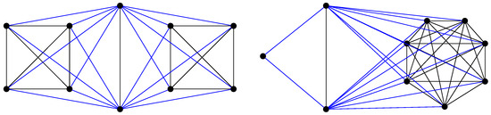
Example 1.

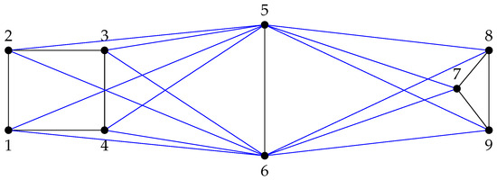
For $\mathcal{H}=P_3$, $G_1=C_4$, $G_2=K_2$ and $G_3=K_3$, the graph $G={\displaystyle \underset{P_3}{\bigvee }}\{G_1,G_2,G_3\}$ is given in the following Figure 2.

Figure 2. $G={\displaystyle \underset{P_3}{\bigvee }}\{C_4,K_2,K_3\}$.

In this example, we have that $k_1=6$, $k_2=8$, $k_3=6$ and

$$L_1=\left[\begin{array}{rrrr}\hfill 6& -1& \hfill -\frac{1}{2}& -1\\ \hfill -1& 6& \hfill -1& -\frac{1}{2}\\ \hfill -\frac{1}{2}& -1& \hfill 6& -1\\ \hfill -1& -\frac{1}{2}& \hfill -1& 6\end{array}\right]L_2=\left[\begin{array}{rr}\hfill 8& -1\\ \hfill -1& 8\end{array}\right]L_3=\left[\begin{array}{rrr}\hfill 6& -1& \hfill -1\\ \hfill -1& 6& \hfill -1\\ \hfill -1& -1& \hfill 6\end{array}\right].$$

Thus, $\sigma \left(R{L}_1\right)=\{\frac{7}{2},{\frac{13}{2}}^{\left[2\right]},\frac{15}{2}\}$, $\sigma \left(R{L}_2\right)=\{7,9\}$, $\sigma \left(R{L}_3\right)=\{4,7^{\left[2\right]}\}$ where ${\lambda }^{\left[t\right]}$ denotes that λ is an eigenvalue with multiplicity t. Moreover

$$F_3=\left[\begin{array}{rrr}\hfill \frac{7}{2}& -2& -\frac{3}{2}\\ \hfill -4& 7& -3\\ \hfill -2& -2& 4\end{array}\right]$$

and $\sigma \left(F_3\right)=\{9,\frac{11}{2},0\}$. Applying Theorem 9, we obtain

$$\sigma \left(RL\left(G\right)\right)=\left\{9^{\left[2\right]},\frac{15}{2},7^{\left[2\right]},{\frac{13}{2}}^{\left[2\right]},\frac{11}{2},0\right\}.$$

A wheel graph on $n\ge 4$ vertices, denoted by $W_n$, is a graph formed by connecting a single vertex to all vertices of a cycle of order $n-1$. We observe that $W_n=K_1\vee C_{n-1}$.

A generalized wheel graph on n vertices, denoted by $G{W}_{a,n-a}$, is a graph consisting of an independent set of order a and a cycle of the remaining $n-a$ vertices, such that each vertex in the cycle is adjacent to every vertex in the independent set. We can write this graph as

$$G{W}_{a,n-a}=\overline{K_a}\bigvee C_{n-a}=\underset{S_{a+1}}{\bigvee }\{C_{n-a},K_1,K_1,\dots ,K_1\}.$$

The $\overline{K_a}$ is not a connected graph, and since we define the join product for connected graphs, so that the distance between the components is not indeterminate, then we will use the following notation

$$G{W}_{a,n-a}=\underset{S_{a+1}}{\bigvee }\{C_{n-a},K_1,K_1,\dots ,K_1\}.$$

Proposition 4.

Let $G{W}_{a,n-a}$ be a generalized wheel graph on n vertices. Then the eigenvalues of $RL\left(G{W}_{a,n-a}\right)$ are $n,0,{\frac{2n-a}{2}}^{[a-1]}$ and the eigenvalues of the form $\left(\frac{n+a+2}{2}-cos\left(\frac{2\pi (n-a+1-j)}{n-a}\right)\right)$ for $j=2,\dots ,n-a$.

Proof. 

In the generalized join operation

$$G{W}_{a,n-a}=\underset{S_{a+1}}{\bigvee }\{C_{n-a},K_1,K_1,\dots ,K_1\},$$

we associate the cycle to the central vertex of the star and each vertex $K_1$ is associated to the pending vertices of the star. Considering the labeling in this same order, we have that the expressions given in (2) and (3), for the graph $G{W}_{a,n-a}$, are

$$\begin{array}{ccc}\hfill RL\left(G{W}_{a,n-a}\right)& =& \left[\begin{array}{ccccc}{L}_1& -J_{n-a\times 1}& -J_{n-a\times 1}& \dots & -J_{n-a\times 1}\\ -J_{1\times n-a}& L_2& -\frac{1}{2}& \dots & -\frac{1}{2}\\ -J_{1\times n-a}& -\frac{1}{2}& L_3& \ddots & ⋮\\ ⋮& ⋮& \ddots & \ddots & -\frac{1}{2}\\ -J_{1\times n-a}& -\frac{1}{2}& \dots & -\frac{1}{2}& L_{a+1}\end{array}\right]\hfill \end{array}$$

where

$$L_1=\frac{n+a+1}{2}{I}_{n-a}+-(J_{n-a}-I_{n-a}+A\left(C_{n-a}\right)),$$

and

$$L_2=\dots =L_{a+1}=\left[\frac{2n-a-1}{2}\right]$$

are matrices of order $1\times 1$. Now, expression (4) for $L_1$ becomes

$$\sigma \left(L_1\right)=\left\{a,\frac{n+a+2}{2}-\frac{1}{2}{\lambda }_{n-a}\left(A\left(C_{n-a}\right)\right),\dots ,\frac{n+a+2}{2}-\frac{1}{2}{\lambda }_2\left(A\left(C_{n-a}\right)\right)\right\},$$

Since the adjacency eigenvalues of the cycle of order p have the form $cos\left(\frac{2\pi (p+1-j)}{p}\right)$, then, from Theorem 9, for $j=2,\dots ,n-a$, we have that $\left(\frac{n+a+2}{2}-cos\left(\frac{2\pi (n-a+1-j)}{n-a}\right)\right)$ are eigenvalues of $RL\left(G{W}_{a,n-a}\right)$.

Now, the matrix $F_s$ given in Theorem 9 has the form

$$F_{a+1}=\left[\begin{array}{cccccc}a& -1& -1& \dots & -1& -1\\ -(n-a)& \frac{2n-a-1}{2}& -\frac{1}{2}& \dots & -\frac{1}{2}& -\frac{1}{2}\\ -(n-a)& -\frac{1}{2}& \frac{2n-a-1}{2}& \dots & -\frac{1}{2}& -\frac{1}{2}\\ ⋮& ⋮& & \ddots & & ⋮\\ -(n-a)& -\frac{1}{2}& -\frac{1}{2}& \dots & \frac{2n-a-1}{2}& -\frac{1}{2}\\ -(n-a)& -\frac{1}{2}& -\frac{1}{2}& \dots & -\frac{1}{2}& \frac{2n-a-1}{2}\end{array}\right].$$

(5)

We recall that ${\mathbf{e}}_i$ denotes the i-th canonical vector. Then, for $i=3,\dots ,a+1$

$$F_{a+1}[{\mathbf{e}}_2-{\mathbf{e}}_{2+i}]=\frac{2n-a}{2}\left[{\mathbf{e}}_2-{\mathbf{e}}_{2+i}\right].$$

Thus, $\frac{2n-a}{2}$ is an eigenvalue of $F_{a+1}$ with multiplicity $a-1$. From Theorem 9, we have that $\frac{2n-a}{2}$ is an eigenvalue of $RL\left(G{W}_{a,n-a}\right)$ with multiplicity $a-1$. From Corollary 3, we have that the largest and smallest eigenvalues of $RL\left(G\right)$ are the largest and smallest eigenvalues of $F_{a+1}$ matrix given in (5). Then, we obtain the spectral radius applying the fact that the trace of the matrix is equal to the sum of its eigenvalues. This fact, applied to the matrix $F_{a+1}$, gives us that $\rho \left(RL\left(G{W}_{a,n-a}\right)\right)=n$. □

An immediate consequence is the following result.

Corollary 4.

Let $W_n$ be a wheel graph on n vertices. Then, the eigenvalues of $RL\left(W_n\right)$ are $n,0$ and the eigenvalues of the form $\left(\frac{n+3}{2}-cos\left(\frac{2\pi (n-j)}{n-1}\right)\right)$ for $j=2,\dots ,n-1$.

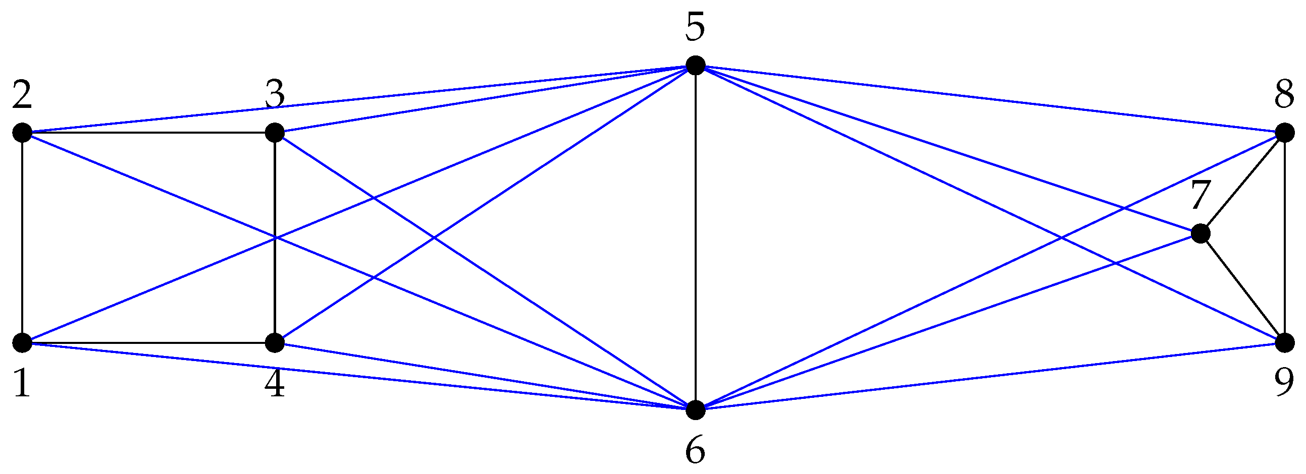
Example 2.

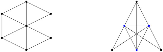
Consider the wheel graph $W_7=K_1\vee C_6$ (see Figure 3). The spectrum $\sigma \left(RL\left(W_7\right)\right)=\{7,6,{\left(\frac{9}{2}\right)}^{\left[2\right]},{\left(\frac{9}{11}\right)}^{\left[2\right]},0\}$. In fact, verifying the expressions given in Corollary 4, we see that

$$\begin{array}{cccc}{\lambda }_1=& 7,& {\lambda }_7=& 0\end{array}$$

and, for $j=2,\dots ,6$, so we apply the expression

$${\lambda }_j=\frac{n+3}{2}-cos\left(\frac{2\pi (n-j)}{n-1}\right).$$

Figure 3. The image shows on the left side the wheel graph of order 7, denoted by $W_7$, and on the right side it shows the generalized wheel graph of order 6 and with $a=3$, denoted by $G{W}_{3,3}$ (where the vertices of $C_3$ are highlighted in blue).

Thus, we have

$$\begin{array}{cc}{\lambda }_2=\hfill & \frac{7+3}{2}-cos\left(\frac{2\pi (7-2)}{7-1}\right)=\frac{9}{2}\hfill \\ {\lambda }_3=\hfill & \frac{7+3}{2}-cos\left(\frac{2\pi (7-2)}{7-3}\right)=\frac{11}{2}\hfill \\ {\lambda }_4=\hfill & \frac{7+3}{2}-cos\left(\frac{2\pi (7-4)}{7-1}\right)=6\hfill \\ {\lambda }_5=\hfill & \frac{7+3}{2}-cos\left(\frac{2\pi (7-5)}{7-1}\right)=\frac{11}{2}\hfill \\ {\lambda }_6=\hfill & \frac{7+3}{2}-cos\left(\frac{2\pi (7-6)}{7-1}\right)=\frac{9}{2}.\hfill \end{array}$$

Example 3.

Consider the following generalized wheel graph with $a=3$, $G{W}_{3,3}={\displaystyle \underset{S_4}{\bigvee }}\{C_3,K_1,K_1,K_1\}$ (see Figure 3). The spectrum $\sigma \left(RL\left(G{W}_{3,3}\right)\right)=\{6^{\left[3\right]},{\left(\frac{9}{2}\right)}^{\left[2\right]},0\}.$ Verifying the expressions given in Proposition 4, we obtain

$$\begin{array}{ccccc}{\lambda }_1=6,& {\lambda }_4=\frac{9}{2},& {\lambda }_5=\frac{9}{2}& \mathit{and}& {\lambda }_6=0.\end{array}$$

For $j=2,3$ applying the expression

$${\lambda }_j=\frac{n+a+2}{2}-cos\left(\frac{2\pi (n-a+1-j)}{n-a}\right)$$

we have

$$\begin{array}{cc}{\lambda }_2=\hfill & \frac{6+3+2}{2}-cos\left(\frac{2\pi (6-3+1-2)}{6-3}\right)=6\hfill \\ {\lambda }_3=\hfill & \frac{6+3+2}{2}-cos\left(\frac{2\pi (6-3+1-3)}{6-3}\right)=6.\hfill \end{array}$$

3. Bounds for Harary Laplacian-Energy-like

In this section, we obtain upper and lower bounds of Harary Laplacian-energy-like of a graph, in terms of the other invariants of the graph.

Remark 2.

If $\tilde{G}$ is the connected graph obtained from G by the deletion of an edge, then from definition of the reciprocal distance Laplacian matrix, we obtain that $trace\left(RL\left(\tilde{G}\right)\right)<trace\left(RL\left(G\right)\right)$.

An immediate consequence due to the Theorem 3 is the following result.

Corollary 5.

If G and $\tilde{G}$ are connected graphs such that $\tilde{G}$ is obtained from G by the deletion of an edge, then

$$HLEL\left(\tilde{G}\right)<HLEL\left(G\right).$$

From Corollary 5 and Remark 1, we obtain the following result.

Corollary 6.

Among the all connected graphs on n vertices and $m\ge n$ edges, the complete graph $K_n$ has the largest Harary Laplacian-energy-like. Thus

$$HLEL\left(G\right)\le (n-1)\sqrt{n}$$

with equality if and only if $G=K_n$.

In the following Theorem, we obtain an upper bound of Harary Laplacian-energy-like in terms of the number of vertices and the Harary index.

Theorem 10.

Let G be a connected graph of order $n\ge 2$ and Harary index $H\left(G\right)$. Then

$$\begin{array}{c}\hfill HLEL\left(G\right)\le \sqrt{2H\left(G\right)+n(n-1)(n-2)},\end{array}$$

with equality if and only if $G=K_n$.

Proof. 

Let G be a connected graph of order $n\ge 2$. We have

$$\begin{array}{cc}\hfill {\left(HLEL\left(G\right)\right)}^2& ={\left(\sum _{i=1}^{n-1}\sqrt{{\lambda }_i\left(RL\left(G\right)\right)}\right)}^2\hfill \\ \hfill & =\sum _{i=1}^{n-1}{\lambda }_i\left(RL\left(G\right)\right)+2\sum _{i\ne j}\sqrt{{\lambda }_i\left(RL\left(G\right)\right)}\sqrt{{\lambda }_j\left(RL\left(G\right)\right)}.\hfill \end{array}$$

(6)

From Theorem 3 and Remark 1, we obtain

$$\begin{array}{c}\hfill \rho \left(RL\left(G\right)\right)\le \rho \left(RL\left(K_n\right)\right)=n,{\lambda }_i\left(RL\left(G\right)\right)\le {\lambda }_i\left(RL\left(K_n\right)\right)=n,i\ge 2.\end{array}$$

Now,

$$\begin{array}{cc}\hfill \sum _{i\ne j}\sqrt{{\lambda }_i\left(RL\left(G\right)\right)}\sqrt{{\lambda }_j\left(RL\left(G\right)\right)}=& \sqrt{{\lambda }_1\left(RL\left(G\right)\right)}(\sqrt{{\lambda }_2\left(RL\left(G\right)\right)}+\dots +\sqrt{{\lambda }_{n-1}\left(RL\left(G\right)\right)})\hfill \\ \hfill & +\sqrt{{\lambda }_2\left(RL\left(G\right)\right)}(\sqrt{{\lambda }_3\left(RL\left(G\right)\right)}+\dots +\sqrt{{\lambda }_{n-1}\left(RL\left(G\right)\right)})\hfill \\ \hfill & +\dots +\sqrt{{\lambda }_{n-2}\left(RL\left(G\right)\right)}\sqrt{{\lambda }_{n-1}\left(RL\left(G\right)\right)}\hfill \\ \hfill \le & \sqrt{n}\left((n-2)\sqrt{n}\right)+\sqrt{n}\left((n-3)\sqrt{n}\right)+\dots +\sqrt{n}\sqrt{n}\hfill \\ \hfill =& n\sum _{i=1}^{n-2}i=\frac{n(n-1)(n-2)}{2}.\hfill \end{array}$$

Replacing Equation (6), we obtain

$$\begin{array}{c}\hfill HLEL\left(G\right)\le \sqrt{2H\left(G\right)+n(n-1)(n-2)}.\end{array}$$

We observe that the equality occurs if and only if ${\rho }_1\left(G\right)=n$ and ${\lambda }_i\left(RL\left(G\right)\right)=n$, for all $2\le i\le n-1$. Applying Theorem 2, we obtain that $G=K_n$. □

An upper bound of Harary Laplacian-energy-like in terms of the number of vertices, Harary index and the Frobenius norm of reciprocal distance Laplacian matrix of graph G are obtained.

Theorem 11.

Let G be a graph of order $n\ge 2$. Then

$$\begin{array}{c}\hfill HLEL\left(G\right)\le \sqrt{\frac{{\left|\right|RL\left(G\right)\left|\right|}_F^2}{2H\left(G\right)}}+\sqrt{(n-2)\left(2H\left(G\right)-\frac{{\left|\right|RL\left(G\right)\left|\right|}_F^2}{2H\left(G\right)}\right)}.\end{array}$$

The equality holds if and only if $G=K_n$.

Proof. 

We observe that $HLEL\left(G\right)=\sqrt{\rho \left(RL\right(G\left)\right)}+{\displaystyle \sum _{i=2}^{n-1}}\sqrt{{\lambda }_i\left(RL\left(G\right)\right)}$. Using the Cauchy–Schwartz’s inequality, we obtain

$$\begin{array}{c}\hfill {\left(HLEL\left(G\right)-\sqrt{\rho \left(RL\right(G\left)\right)}\right)}^2\le (n-2)\sum _{i=2}^{n-1}{\lambda }_i\left(RL\left(G\right)\right).\end{array}$$

(7)

Thus

$$\begin{array}{c}\hfill HLEL\left(G\right)\le \sqrt{\rho \left(RL\right(G\left)\right)}+\sqrt{(n-2)\left(2H\right(G)-\rho (RL\left(G\right)\left)\right)}.\end{array}$$

Let $m\left(x\right)=\sqrt{x}+\sqrt{(n-2)\left(2H\right(G)-x)}$ be a real function. We recall that $m\left(x\right)$ is a strictly decreasing function in the interval $\left[\frac{2H\left(G\right)}{n-1},2H\left(G\right)\right]$.

We observe that $\rho \left(RL\right(G\left)\right)<2H\left(G\right)$ and

$$\begin{array}{c}\hfill \frac{2H\left(G\right)}{n-1}=\frac{{\left(2H\left(G\right)\right)}^2}{(n-1)2H\left(G\right)}\le \frac{{\displaystyle \sum _{i=1}^{n-1}}{\lambda }_i{\left(RL\left(G\right)\right)}^2}{2H\left(G\right)}=\frac{{\left|\right|RL\left(G\right)\left|\right|}_F^2}{2H\left(G\right)}.\end{array}$$

Then, using Theorem 6, we have

$$\frac{2H\left(G\right)}{n-1}\le \frac{{\left|\right|RL\left(G\right)\left|\right|}_F^2}{2H\left(G\right)}\le \rho \left(RL\left(G\right)\right)<2H\left(G\right).$$

Therefore

$$\begin{array}{c}\hfill HLEL\left(G\right)\le \sqrt{\frac{{\left|\right|RL\left(G\right)\left|\right|}_F^2}{2H\left(G\right)}}+\sqrt{(n-2)\left(2H\left(G\right)-\frac{{\left|\right|RL\left(G\right)\left|\right|}_F^2}{2H\left(G\right)}\right)}.\end{array}$$

Now, we observe that the equality holds whenever the equality (7) and the bound given in Theorem 6 hold. In the first case, the equality occurs if

$$\rho \left(RL\left(G\right)\right)={\lambda }_2\left(RL\left(G\right)\right)=\dots ={\lambda }_{n-1}\left(RL\left(G\right)\right),$$

and thus the multiplicity of $\rho \left(RL\right(G\left)\right)$ is $n-1$ and, using Theorem 2, we conclude that $G=K_n$. In the second case, the equality in Theorem 6 occurs if $G=K_n$. Reciprocally, if $G=K_n$ with $n\ge 2$, then

$$\begin{array}{c}\hfill \sqrt{\frac{{\left|\right|RL\left(G\right)\left|\right|}_F^2}{2H\left(G\right)}}+\sqrt{(n-2)\left(2H\left(G\right)-\frac{{\left|\right|RL\left(G\right)\left|\right|}_F^2}{2H\left(G\right)}\right)}=(n-1)\sqrt{n}.\end{array}$$

□

The following example shows a comparison of the bounds obtained with the real $HLEL$ values considering various known graphs.

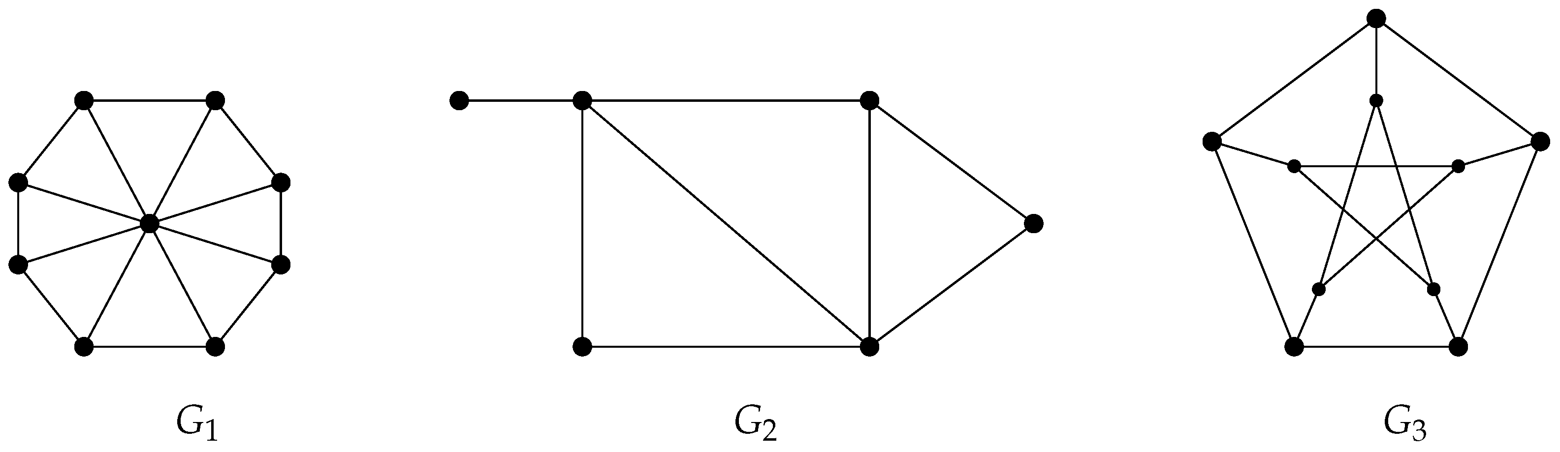
Example 4.

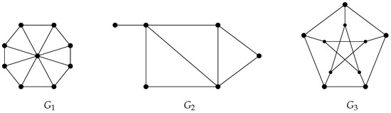
We consider the graphs $G_1$, $G_2$ given by Figure 4. Let $G_3$ be the Petersen graph and let $G_4=S_7$, $G_5=P_7$ and $G_6=C_7$ be the star, path and cycle on seven vertices, respectively.

Figure 4. Examples of connected simple undirected graphs.

Using four decimal places, in Table 1 we show the upper bounds obtained for Harary Laplacian-energy-like for the given graphs.

Table 1. Examples of the upper bounds obtained for Harary Laplacian-energy-like.

	${\mathit{G}}_{\mathbf{1}}$	${\mathit{G}}_{\mathbf{2}}$	${\mathit{G}}_{\mathbf{3}}$	${\mathit{S}}_{\mathbf{7}}$	${\mathit{P}}_{\mathbf{7}}$	${\mathit{C}}_{\mathbf{7}}$
$HLEL\left(G\right)$	$20.3256$	$10.5869$	$23.2019$	$11.5900$	$11.4529$	$12.3590$
Corollary 6	$24.0000$	$12.2475$	$28.4605$	$15.8745$	$15.8745$	$15.8745$
Theorem 10	$23.5797$	$11.9443$	$27.9285$	$15.3948$	$15.2414$	$15.3514$
Theorem 11	$20.3958$	$10.6452$	$23.2378$	$12.7267$	$11.5658$	$12.4094$

Lemma 3

([25]). Let m and n be natural numbers such that $m\ge n>2$. Let $a_1,a_2,\dots ,a_m$ be positive real numbers. Then,

$$\frac{2}{n}{\left(\sum _{i=1}^m{a}_i\right)}^2>\sum _{i=1}^m{a}_i^2.$$

Theorem 12.

Let G be a graph of order $n>2$. Then

$$HLEL\left(G\right)>\sqrt{(n-1)H\left(G\right)}.$$

Proof. 

Applying Lemma 3 to the definition of $HLEL\left(G\right)$, we obtain

$${\left(HLEL\left(G\right)\right)}^2>\frac{n-1}{2}\sum _{i=1}^{n-1}{\lambda }_i\left(RL\left(G\right)\right)=(n-1)H\left(G\right).$$

Therefore,

$$HLEL\left(G\right)>\sqrt{(n-1)H\left(G\right)}.$$

□

Example 5.

The Table 2 shows, to four decimal places, the lower bound obtained for Harary Laplacian-energy-like for the graphs given in Example 4.

Table 2. Examples of the lower bounds obtained for Harary Laplacian-energy-like.

	${\mathit{G}}_{\mathbf{1}}$	${\mathit{G}}_{\mathbf{2}}$	${\mathit{G}}_{\mathbf{3}}$	${\mathit{S}}_{\mathbf{7}}$	${\mathit{P}}_{\mathbf{7}}$	${\mathit{C}}_{\mathbf{7}}$
$HLEL\left(G\right)$	$20.3256$	$10.5869$	$23.2019$	$11.5900$	$11.4529$	$12.3590$
Theorem 12	$14.4222$	$7.5277$	$16.4317$	9	$8.1792$	$8.7750$

Now, to begin the end of this section, we recall that the vertex connectivity of a graph G, denoted by $\kappa \left(G\right)$, is the minimum number of vertices of G, the deletion of which disconnects G. Clearly, $\kappa \left(K_n\right)=n-1$. Applying the results of the previous section, we find upper bounds on Harary Laplacian-energy-like among all the connected graphs of prescribed order in terms of the vertex connectivity.

Let $\mathcal{V}(n,k)$ be the family of connected graphs G of order n such that $\kappa \left(G\right)\le k$.

For $i=1,2,3$, let $G_i$ be a ${\delta }_i$-regular graph of order $n_i$. Then $G=G_1\vee (G_2\cup G_3)$ is a graph of order $n=n_1+n_2+n_3$. Observe that

$$G_1\vee (G_2\cup G_3)\equiv \underset{P_3}{\bigvee }\{G_2,G_1,G_3\}$$

and

$$G_1\vee (G_2\cup G_3)\in \mathcal{V}(n,n_1).$$

Labeling the vertices of $G=G_1\vee (G_2\cup G_3)$ starting with the vertices of $G_1$, continuing with the vertices of $G_2$ and finishing with the vertices of $G_3$, and using the results obtained in the previous subsection, the reciprocal distance Laplacian matrix $RL\left(G\right)$ becomes

$$RL\left(G\right)=\left[\begin{array}{ccc}{L}_1& -J_{n_1\times n_2}& -J_{n_1\times n_3}\\ -J_{n_2\times n_1}& L_2& \frac{-1}{2}{J}_{n_2\times n_3}\\ -J_{n_3\times n_1}& \frac{-1}{2}{J}_{n_3\times n_2}& L_3\end{array}\right]$$

where for $i=1,2,3,$

$$L_i=k_i{I}_{n_i}-\frac{1}{2}\left(J_{n_i}-I_{n_i}+A\left(G_i\right)\right)$$

(8)

and

$$\begin{array}{ccc}\hfill k_1& =& \frac{1}{2}(n_1-1)+\frac{1}{2}{\delta }_1+n_2+n_3\hfill \\ \hfill k_2& =& \frac{1}{2}(n_2-1)+\frac{1}{2}{\delta }_2+n_1+\frac{1}{2}{n}_3\hfill \\ \hfill k_3& =& \frac{1}{2}(n_3-1)+\frac{1}{2}{\delta }_3+n_1+\frac{1}{2}{n}_2.\hfill \end{array}$$

The eigenvalues of $L_1$, $L_2$ and $L_3$ associated to ${\mathbf{e}}_{n_1},{\mathbf{e}}_{n_2}$ and ${\mathbf{e}}_{n_3}$, respectively, are

$${\lambda }_l\left(L_1\right)=n_2+n_3,{\lambda }_l\left(L_2\right)=n_1+\frac{1}{2}{n}_{3}and{\lambda }_l\left(L_3\right)=n_1+\frac{1}{2}{n}_2$$

(9)

Using these observations, the following result is due to applying Theorem 9.

Proposition 5.

If $G=G_1\vee (G_2\cup G_3)$ and, for $i=1,2,3$, $G_i$ is a ${\delta }_i$-regular graph then

$$\sigma \left(L\left(G\right)\right)=(\sigma \left(L_1\right)\cup \sigma \left(L_2\right)\cup \sigma \left(L_3\right)-\{{\lambda }_l\left(L_1\right),{\lambda }_l\left(L_2\right),{\lambda }_l\left(L_3\right)\})\cup \sigma \left(F_3\right)$$

where $L_1,L_2,L_3$ are as in (8), ${\lambda }_l\left(L_1\right),{\lambda }_l\left(L_2\right),{\lambda }_l{L}_3)$ are as in (9) and

$$F_3=\left[\begin{array}{ccc}{\lambda }_l\left(L_1\right)& -n_2& -n_3\\ -n_1& {\lambda }_l\left(L_2\right)& -\frac{1}{2}{n}_3\\ -n_1& -\frac{1}{2}{n}_2& {\lambda }_l\left(L_3\right)\end{array}\right]$$

(10)

Let n and k be positive integers, with $k\le n-1$ and consider the graph

$$G\left(j\right)=K_k\vee (K_j\cup K_{n-k-j})$$

where, without loss of generality, we assume $1\le j\le \lfloor \frac{n-k}{2}\rfloor$. The following result is obtained by applying Proposition 5 to $RL\left(G\right(j\left)\right)$.

Proposition 6.

Let $G\left(j\right)=K_k\vee (K_j\cup K_{n-k-j})$ such that $1\le j\le \lfloor \frac{n-k}{2}\rfloor$. Then

$$\begin{array}{ccc}\hfill \sigma \left(RL\right(G\left(i\right)\left)\right)& =& \left\{n^{\left[k\right]},\frac{n+k}{2},{\left(\frac{n+k+j}{2}\right)}^{[j-1]},{\left(\frac{2n-j}{2}\right)}^{[n-k-j-1]},0\right\}\hfill \end{array}$$

In particular,

$$\begin{array}{ccc}\hfill HLEL(K_k\vee (K_1\cup K_{n-k-1}))& =& k\sqrt{n}+\sqrt{\frac{n+k}{2}}+(n-k-2)\sqrt{\frac{2n-1}{2}}.\hfill \end{array}$$

Proof. 

We observe that for the graph $G\left(j\right)=K_k\vee (K_j\cup K_{n-k-j})$, the matrices $L_1$, $L_2$ and $L_3$ in (8) are

$$\begin{array}{ccc}\hfill L_1& =& (n-1)I_k-A\left(K_k\right)\hfill \\ \hfill L_2& =& \left(\frac{n+k+j-2}{2}\right)I_i-A\left(K_j\right)\hfill \\ \hfill L_3& =& \left(\frac{2n-j-2}{2}\right)I_{n-k-j}-A\left(K_{n-k-j}\right),\hfill \end{array}$$

respectively, and the matrix $F_3\left(G\left(j\right)\right)$ in (10) becomes

$$F_3=\left[\begin{array}{ccc}n-k& -j& -(n-k-j)\\ -k& \frac{n+k-j}{2}& -\frac{n-k-j}{2}\\ -k& -\frac{j}{2}& \frac{k+j}{2}\end{array}\right].$$

Then,

$$\begin{array}{ccc}\hfill \sigma \left(L_1\right)& =& \left\{n^{[k-1]},n-k\right\}\hfill \\ \hfill \sigma \left(L_2\right)& =& \left\{{\left(\frac{n+k+j}{2}\right)}^{[j-1]},\frac{n+k-j}{2}\right\}\hfill \\ \hfill \sigma \left(L_3\right)& =& \left\{{\left(\frac{2n-j}{2}\right)}^{[n-k-j-1]},\frac{2k+j}{2}\right\}\hfill \end{array}$$

and the spectrum of $F_3\left(G\left(j\right)\right)$ is

$$\sigma \left(F_3\left(G\left(j\right)\right)\right)=\left\{n,\frac{n+k}{2},0\right\}.$$

Since

$$HLEL\left(G\right)=\sum _{i=1}^{n-1}\sqrt{{\lambda }_i\left(RL\left(G\right)\right)}.$$

The result is obtained. □

Let

$$\mathcal{W}(n,k)=\{G\in V(n,k):|E\left(G\right)|\ge n\}.$$

and let

$$\begin{array}{ccc}\hfill c(n,k)& =& k\sqrt{n}+\sqrt{\frac{n+k}{2}}+(n-k-2)\sqrt{\frac{2n-1}{2}}.\hfill \end{array}$$

If, $K_0$ denotes the empty graph, i.e., the graph without edges and without vertices, then we have the following results.

Lemma 4.

Let $G\left(j\right)=K_k\vee (K_j\cup K_{n-k-j})$ for $1\le j\le \lfloor \frac{n-k}{2}\rfloor$. Then

$$HLEL\left(G\left(⌊\frac{n-k}{2}⌋\right)\right)\le HLEL\left(G\left(j\right)\right)\le HLEL\left(G\left(1\right)\right).$$

Proof. 

From Proposition 6, we have

$$HLEL\left(G\left(j\right)\right)=k\sqrt{n}+\sqrt{\frac{n+k}{2}}+(j-1)\sqrt{\frac{n+k+j}{2}}+(n-k-j-1)\sqrt{\frac{2n-j}{2}}.$$

We define the function

$$f\left(x\right)=(x-1)\sqrt{\frac{n+k+x}{2}}+(n-k-x-1)\sqrt{\frac{2n-x}{2}}.$$

We observe that $f\left(x\right)=f(n-k-x)$ for $x\in [0,n-k]$ and f is a strictly decreasing function in the interval

$$\left[\frac{n-k}{2}-\frac{\sqrt{(k+7n-2)(5k+11n+2)}}{6},\frac{n-k}{2}\right]\supset \left[1,\frac{n-k}{2}\right].$$

Thus, the result is obtained. □

Theorem 13.

If $G\in \mathcal{W}(n,k)$, then

$$HLEL\left(G\right)\le c(n,k),fork=1,\dots ,n-1.$$

(11)

Additionally, the equality in (11) holds if and only is $G=K_k\vee (K_1\cup K_{n-k-1})$.

Proof. 

Let $G\in \mathcal{W}(n,k)$. We first consider $k=n-1$. From Corollary 6, $HLEL\left(G\right)\le HLEL\left(K_n\right)$ with equality if and only if $G=K_n$. Furthermore

$$c(n,n-1)=(n-1)\sqrt{n}=HLEL\left(K_n\right).$$

Then, the result is true for $k=n-1$. Now, let $1\le k\le n-2$ and let $G\in \mathcal{W}(n,k)$ such that $HLEL\left(G\right)$ is a maximum.

Let $S\subseteq V\left(G\right)$ such that $G\setminus S$ is a disconnected graph and $\left|S\right|=\kappa \left(G\right)$. We denote by $C_1,C_2,\dots ,C_r$ the r connected components of $G\setminus S$. Clearly $r\ge 2$. Suppose that $r>2$, then we can construct a new graph $G\cup \left\{e\right\}$ where e is an edge connecting a vertex in $C_1$ with a vertex in $C_2$. We can see that $G\cup \left\{e\right\}\in W(n,k)$. Using Corollary 5, we have

$$HLEL\left(G\right)<HLEL(G\cup \{e\left\}\right).$$

It is a contradiction because G is the graph with maximum $HLEL$. Therefore $r=2$, that is, $G\setminus S=C_1\cup C_2$.

By definition $\left|S\right|\le k$. Now, we claim that $\left|S\right|=k$.

Suppose $\left|S\right|<k$. Since $G\setminus S=C_1\cup C_2$, we may construct a graph $H=G\cup \left\{e\right\}$ where e is an edge joining a vertex $u\in V\left(C_1\right)$ with a vertex $v\in V\left(C_2\right)$. We see that $H\setminus S$ is a connected graph and the deletion of the vertex u disconnected it, and then $H\in \mathcal{W}(n,k)$. Using Corollary 5, $HLEL\left(G\right)<HLEL\left(H\right)$, which is also a contradiction. Hence, $G\setminus S=C_1\cup C_2$ and $\left|S\right|=k$. Let $|C_1|=j$. Then $|C_2|=n-k-j$. Through the repeated application of Corollary 5, we can conclude that

$$G=K_k\vee (K_j\cup K_{n-k-j})=G\left(j\right)$$

for some $1\le i\le \lfloor \frac{n-k}{2}\rfloor$. We have proved $HLEL\left(G\right)\le HLEL\left(G\right(i\left)\right)$ for all $G\in W(n,k)$. From Lemma 4, we have that $HLEL\left(G\right(i\left)\right)\le HLEL\left(G\right(1\left)\right)$. Since $HLEL\left(G\right(1\left)\right)=c(n,k)$, for $k=1,\dots ,n-1$, the equality holds if and only if $G=K_k\vee (K_1\cup K_{n-k-1})$. □

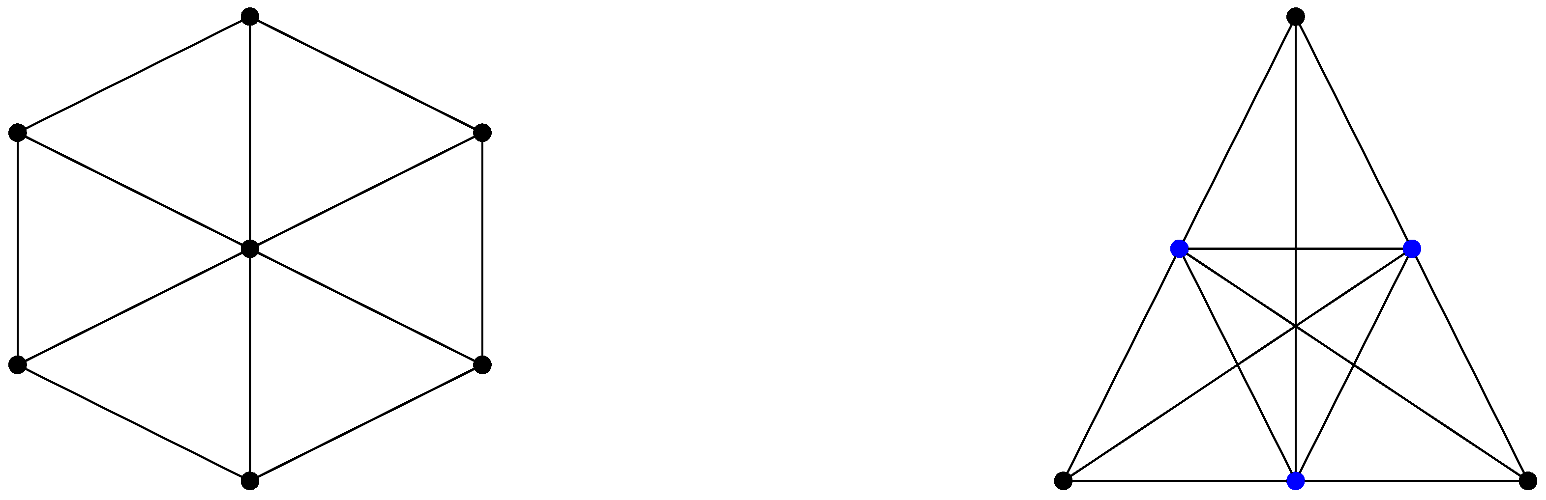
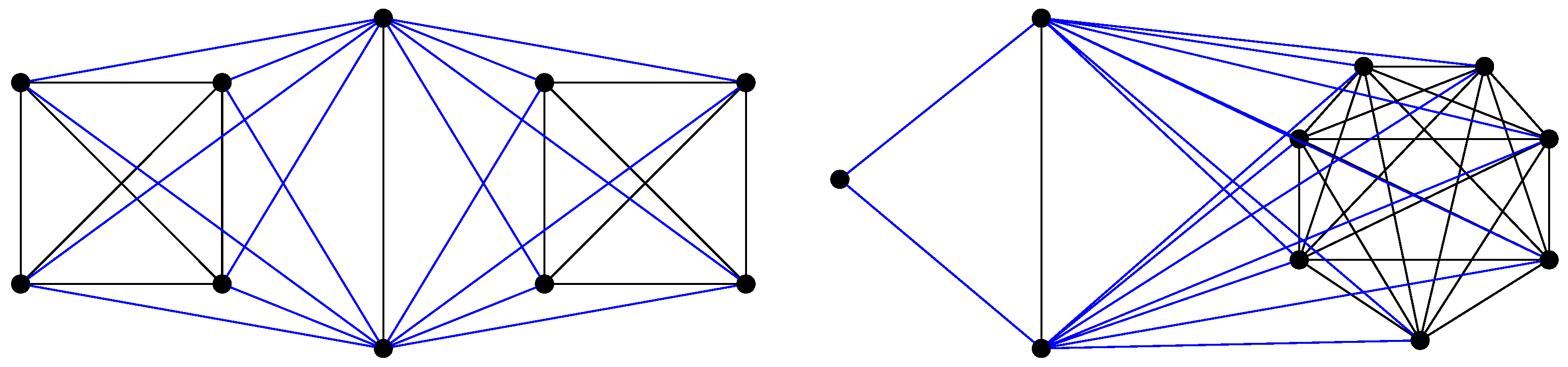
Example 6.

For $n=10$ and $k=2$, the graphs with minimum and maximum Harary Laplacian-energy-like are $G_1=K_2\vee (K_4\cup K_4)$ and $G_2=K_2\vee (K_1\cup K_7)$, respectively (see Figure 5). In fact, using four decimal places,

$$HLEL\left(K_2\vee (K_4\cup K_4)\right)=25.7446\mathit{and}HLEL\left(K_2\vee (K_1\cup K_7)\right)=27.2673.$$

Figure 5. The graphs $G_1=K_2\vee (K_4\cup K_4)$ and $G_2=K_2\vee (K_1\cup K_7)$.

4. Conclusions

We obtain new spectral results from the Laplacian version of the Harary matrix, known as the Laplacian matrix of the reciprocal of the distance, reducing the order of the matrices from which the eigenvalues are obtained and, in several cases, all the eigenvalues are explicitly provided. We introduce the concept of Harary Laplacian-energy-like, we obtain bounds for this energy and we find extreme graphs for the minimum and maximum values that this energy has for certain families of graphs.

References

- Gutman, I. The Energy of a Graph: Old and New Results. In Algebraic Combinatorics and Applications; Betten, A., Kohnert, A., Laue, R., Wassermann, A., Eds.; Springer: Berlin/Heidelberg, Germany, 2001; pp. 196–211. [Google Scholar]
- Gutman, I.; Furtula, B. The total π-electron energy saga. Croat. Chem. Acta 2017, 90, 359–368. [Google Scholar] [CrossRef]
- Li, X.; Shi, Y.; Gutman, I. Graph Energy; Springer: New York, NY, USA, 2012. [Google Scholar]
- Gutman, I. The energy of a graph. Ber. Math. Statist. Sekt. Forschungsz. Graz 1978, 103, 1–22. [Google Scholar]
- Aashtab, A.; Akbari, S.; Ghasemian, E.; Ghodrati, A.H.; Hosseinzadeh, M.A.; Koorepazan-Moftakhar, F. On the minimum energy of regular graphs. Linear Algebra Appl. 2019, 581, 51–71. [Google Scholar] [CrossRef]
- Das, K.C.; Mojallal, S.A.; Sun, S. On the sum of the k largest eigenvalues of graphs and maximal energy of bipartite graphs. Linear Algebra Appl. 2019, 569, 175–194. [Google Scholar] [CrossRef]
- Zhu, J.; Yang, J. Minimal energies of trees with three branched vertices. MATCH Commun. Math. Comput. Chem. 2018, 79, 263–274. [Google Scholar]
- Alawiah, N.; Rad, N.J.; Jahanbani, A.; Kamarulhaili, H. New upper bounds on the energy of a graph. MATCH Commun. Math. Comput. Chem. 2018, 79, 287–301. [Google Scholar]
- Jahanbani, A. Upper bounds for the energy of graphs. MATCH Commun. Math. Comput. Chem. 2018, 79, 275–286. [Google Scholar]
- Jahanbani, A.; Rodriguez, J. Koolen-Moulton-Type Upper Bounds on the Energy of a Graph. MATCH Commun. Math. Comput. Chem. 2020, 83, 497–518. [Google Scholar]
- Oboudi, M.R. A new lower bound for the energy of graphs. Linear Algebra Appl. 2019, 590, 384–395. [Google Scholar] [CrossRef]
- Das, K.C.; Mojallal, S.A. On Laplacian energy of graphs. Discret. Math. 2014, 325, 52–64. [Google Scholar] [CrossRef]
- Gutman, I.; Ramane, H. Research on Graph Energies in 2019. MATCH Commun. Math. Comput. Chem. 2020, 84, 277–292. [Google Scholar]
- Phillips, J.D. State factor network analysis of ecosystem response to climate change. Ecol. Complex. 2019, 40, 100789. [Google Scholar] [CrossRef]
- Liu, J.; Liu, B. A Laplacian-energy-like invariant of a graph. MATCH Commun. Math. Comput. Chem. 2008, 59, 355–372. [Google Scholar]
- Stevanovic, D.; Ilic, A.; Onisor, C.; Diudea, M. LEL—A Newly Designed Molecular Descriptor. Acta Chim. Slov. 2009, 56, 410–417. [Google Scholar]
- Ivanciuc, O.; Balaban, T.S.; Balaban, A.T. Reciprocal distance matrix, related local vertex invariants and topological indices. J. Math. Chem. 1993, 12, 309–318. [Google Scholar] [CrossRef]
- Plavsić, D.; Nikolić, S.; Trinajstić, N.; Mihalić, Z. On the Harary index for the characterization of chemical graphs. J. Math. Chem. 1993, 12, 235–250. [Google Scholar] [CrossRef]
- Bapat, R.; Panda, S.K. The Spectral Radius of the Reciprocal Distance Laplacian Matrix of a Graph. Bull. Iran. Math. 2018, 44, 1211–1216. [Google Scholar] [CrossRef]
- Medina, L.; Trigo, M. Upper bounds and lower bounds for the spectral radius of Reciprocal Distance, Reciprocal Distance Laplacian and Reciprocal Distance signless Laplacian matrices. Linear Algebra Appl. 2021, 609, 386–412. [Google Scholar] [CrossRef]
- Medina, L.; Trigo, M. Bounds on the Reciprocal distance energy and Reciprocal distance Laplacian energies of a graph. Linear Multilinear Algebra 2022, 70, 3097–3118. [Google Scholar] [CrossRef]
- Brouwer, A.E.; Haemers, W.H. Spectra of Graphs—Monograph; Springer: Berlin/Heidelberg, Germany, 2011. [Google Scholar]
- You, L.; Yang, M.; So, W.; Xi, W. On the spectrum of an equitable quotient matrix and its application. Linear Algebra Appl. 2019, 577, 21–40. [Google Scholar] [CrossRef]
- Cardoso, D.M.; de Freitas, M.A.A.; Martins, E.; Robbiano, M. Spectra of graphs obtained by a generalization of the join graph operation. Discret. Math. 2013, 313, 733–741. [Google Scholar] [CrossRef]
- Diaz, R.; Rojo, O. Sharp upper bounds on the distance energies of a graph. Linear Algebra Appl. 2018, 545, 55–75. [Google Scholar] [CrossRef]
Disclaimer/Publisher’s Note: The statements, opinions and data contained in all publications are solely those of the individual author(s) and contributor(s) and not of MDPI and/or the editor(s). MDPI and/or the editor(s) disclaim responsibility for any injury to people or property resulting from any ideas, methods, instructions or products referred to in the content. |
© 2023 by the authors. Licensee MDPI, Basel, Switzerland. This article is an open access article distributed under the terms and conditions of the Creative Commons Attribution (CC BY) license (https://creativecommons.org/licenses/by/4.0/).