Painlevé Analysis of the Traveling Wave Reduction of the Third-Order Derivative Nonlinear Schrödinger Equation

Abstract

The second partial differential equation from the Kaup–Newell hierarchy is considered. This equation can be employed to model pulse propagation in optical fiber, wave propagation in plasma, or high waves in the deep ocean. The integrability of the explored equation in traveling wave variables is investigated using the Painlevé test. Periodic and solitary wave solutions of the studied equation are presented. The investigated equation belongs to the class of generalized nonlinear Schrödinger equations and may be used for the description of optical solitons in a nonlinear medium.

1. Introduction

In the present paper, we study the analytical properties of the following partial differential equation

$$\begin{array}{c}i{q}_t+i{q}_{xxx}+3q_x^2{q}^{*}+3q|q_x{|}^2+3{\left|q\right|}^2{q}_{xx}-\\ \\ -{3i\left|q\right|}^2{q}^2{q}_x^{*}-\frac{9i}{2}{\left|q\right|}^4{q}_x=0.\end{array}$$

(1)

where $q(x,t)$ is a complex function, $q^{*}$ is the complex conjugate of q, and x and t are independent variables.

Equation (1) is a third-order partial differential equation, which is the second member of the integrable Kaup–Newell hierarchy. Third- and higher-order equations from this hierarchy have not received as much attention as the second-order equation, which is the first equation of the hierarchy (for papers on that equation, see, for example, refs. [1,2,3,4,5,6,7]). In [8], a model for an integrable system of long lattice waves was derived, which is now known as the second equation of the Kaup–Newell hierarchy (1). In [9], Equation (1) was obtained from the Kaup–Newell scattering formulation. As many integrable hierarchies have appeared (see, for instance, refs. [8,10,11]), their exact solutions have been sought after because exact solutions of integrable hierarchies are able to accurately reflect several physical phenomena, for instance, pulse propagation in optical fiber or high and steep waves in the deep ocean [12,13]. The inverse scattering method was applied to obtain the higher-order soliton matrix and the general expression of the higher-order soliton from the Kaup–Newell hierarchy in [14]. Explicit soliton, rational, positon, breather, and rogue wave solutions of the third-order flow equation from the Kaup–Newell hierarchy were generated by applying the Darboux transformation and the Taylor expansion in [15].

There have also been a number of works devoted to Painlevé analysis of partial differential equations over the years. For instance, in [16], Painlevé analysis for the second-order generalized derivative nonlinear Schrodinger equation was performed. In [17], with the aid of symbolic computation, the Painlevé-integrability of a general two-coupled nonlinear Schrodinger system was systematically examined by carrying out the Painlevé test. Many more papers are devoted not only to the construction of solutions of equations describing optical pulses but also to the study of their analytical properties using the Painlevé test [18,19,20,21], as it helps to understand integrability and obtain local expansions of the solutions in Laurent or Puiseux series. To the best of our knowledge, the traveling wave reduction of Equation (1) has not been tested for integrability using Painlevé analysis. Thus, our objective in this paper is to explore integrability by conducting the Painlevé test of the traveling wave reduction of Equation (1) and finding its exact solutions in the form of solitary and periodic waves.

The present work is organized as follows. In Section 2, Equation (1) is reduced to the system of ordinary differential equations by introducing the traveling wave substitution. In Section 3, we conduct the Painlevé analysis and obtain local expansions of solutions of the system in the Puiseux series. In Section 4, we find exact solutions in the form of periodic and solitary waves.

2. Reduction to the System of Nonlinear Ordinary Differential Equations

It is easy to see that Equation (1) admits the shift transformation group in variables x and t. As a consequence, there exist solutions of Equation (1) in traveling wave variables. Substituting

$$\begin{array}{c}q(x,t)=q\left(z\right),z=x-C_{0}t\end{array}$$

(2)

into Equation (1) yields the following ordinary differential equation:

$$\begin{array}{c}i{q}_{zzz}+3q_z^2{q}^{*}+3q|q_z{|}^2+{3\left|q\right|}^2{q}_{zz}-3i{\left|q\right|}^2{q}^2{q}_z^{*}-\\ -\frac{9i}{2}{\left|q\right|}^4{q}_z-i{C}_0{q}_z=0.\end{array}$$

(3)

where $C_0$ is the speed of a traveling wave. The following sections deal with the analytical properties of Equation (3).

3. Painlevé Test for the System of Ordinary Differential Equations Obtained

Let us look for the solution of Equation (3) in the form

$$q\left(z\right)=y\left(z\right)e^{i\varphi \left(z\right)},$$

(4)

where $y\left(z\right)$ is a real function describing the amplitude of a wave packet.

Substituting (4) into the explored Equation (3) yields the following system of equations for the real and imaginary parts of the resulting expression

$$\begin{array}{c}{C}_{0}y{\varphi }_z-3y_{zz}{\varphi }_z-3y_z{\varphi }_{zz}-y{\varphi }_{zzz}+y{\varphi }_z^3+6y{y}_z^2-3y^3{\varphi }_z^2+\\ \\ +3y^2{y}_{zz}+\frac{3y^5{\varphi }_z}{2}=0,\end{array}$$

(5)

$$\begin{array}{c}3y^3{\varphi }_{zz}-3y{\varphi }_z{\varphi }_{zz}-3y_z{\varphi }_z^2+12y_z{y}^2{\varphi }_z-C_0{y}_z+y_{zzz}-\frac{15y^4{y}_z}{2}=0.\end{array}$$

(6)

Denoting ${\varphi }_z=\psi$, we reduce the order of Equations (5) and (6) as follows

$$\begin{array}{c}3y^2{y}_{zz}+C_{0}y\psi -3y_{zz}\psi -3y_z{\psi }_z-y{\psi }_{zz}+y{\psi }^3+\\ \\ +6y{y}_z^2-3y^3{\psi }^2+\frac{3y^5\psi }{2}=0,\end{array}$$

(7)

$$\begin{array}{c}{y}_{zzz}-3y_z{\psi }^2+12y_z{y}^2\psi -C_0{y}_z-\frac{15y^4{y}_z}{2}-3y\psi {\psi }_z+3y^3{\psi }_z=0.\end{array}$$

(8)

To investigate the integrability of the system of Equations (7) and (8), we apply the Painlevé test. The Painlevé test is an effective technique for studying the analytical properties of ordinary differential equations [16,17,18,19,20,21]. If the system possesses the Painlevé property, then its general solution has no movable critical singular points. In that case, we may expect this system to have enough first integrals to be solvable by quadratures. Whenever a system exhibits the Painlevé property, it is integrable.

The three steps of the Painlevé test were first introduced in [22]. A detailed description of each step of the test with examples can also be found, for instance, in [23,24].

The first step of the Painlevé test involves finding the leading terms of Equations (7) and (8) by substituting

$$y\left(z\right)=y_0{(z-z_0)}^{-p},\psi \left(z\right)={\psi }_0{(z-z_0)}^{-q}$$

(9)

into Equations (7) and (8) and selecting terms with the smallest powers of $z-z_0$, where $z_0$ is an arbitrary singular point of the solution of the differential equation on the complex plane. In Equation (9), p and q represent the power of the first term of the expansion of the solution in the Laurent or Puiseux series. For a system of ODEs to pass the first step of the test, the exponents p and q have to be integers, in which case one can proceed to the second step of the test. However, if p and q turn out to be not integers, but rational, one may also proceed to the second step of the test to check for the weak Painlevé property. The weak Painlevé property allows solutions that possess algebraic branch points, yet when the system enjoys the weak Painlevé property, it still may be integrable [25,26].

Substituting (9) into Equations (7) and (8) and choosing from the resulting expression, the smallest possible powers of $z-z_0$ yields the system of equations for leading terms as follows

$$\begin{array}{c}-3y_{zz}\psi -3y_z{\psi }_z-y{\psi }_{zz}+y{\psi }^3+6y{y}_z^2-3y^3{\psi }^2+3y^2{y}_{zz}+\frac{3y^5\psi }{2}=0,\\ \\ -3y^3{\psi }_z-C_0{y}_z-3y_z{\psi }^2+y_{zzz}-\frac{15y^4{y}_z}{2}+12y_z{y}^2\psi -3y\psi {\psi }_z=0.\end{array}$$

(10)

Substituting (9) into the leading terms (10) yields a cumbersome expression depending on $z-z_0$, $y_0$, and ${\psi }_0$, which we do not present here. Equating all powers of $z-z_0$ in the resulting equation to each other, we obtain that the only viable option for resonances p and q is $p=\frac{1}{2},q=1$. These values represent the dominant behavior around the singularity. However, according to the Painlevé test, these values must be integers. Nevertheless, we can continue with testing the equations analyzed for the weak Painlevé property and looking for Puiseux series expansions of local solutions.

To obtain coefficients $y_0$ and ${\psi }_0$, which correspond to the first term in the series, one has to equate the term at the smallest power of $z-z_0$ in the resulting equation. This yields the following system of algebraic equations:

$$\begin{array}{c}-\frac{23}{4}{\psi }_0{y}_0+y_0{\psi }_0^3+\frac{15}{4}{y}_0^3-3y_0^3{\psi }_0^2+\frac{3}{2}{y}_0^5{\psi }_0=0,\\ \\ \frac{9}{2}{\psi }_0^2{y}_0-9y_0^3{\psi }_0-\frac{15}{8}{y}_0+\frac{15}{4}{y}_0^5=0,\end{array}$$

(11)

the explicit solutions of which are

$$\begin{array}{c}{y}_0^{(1,2)}=\pm (1+i),{\psi }_0^{(1,2)}=\frac{3i}{2},\\ \\ y_0^{(3,4)}=\pm (1-i),{\psi }_0^{(3,4)}=-\frac{3i}{2},\\ \\ y_0^{(5,6)}=\pm (1+i),{\psi }_0^{(5,6)}=\frac{5i}{2},\\ \\ y_0^{(7,8)}=\pm (1-i),{\psi }_0^{(7,8)}=-\frac{5i}{2},\\ \\ y_0^{(9,10)}=\pm \sqrt{2}(1+i),{\psi }_0^{(9,10)}=\frac{5i}{2},\\ \\ y_0^{(11,12)}=\pm \sqrt{2}(1-i),{\psi }_0^{(11,12)}=-\frac{5i}{2}.\end{array}$$

(12)

In the second step, we determine the Fuchs indices by substituting

$$\begin{array}{c}y\left(z\right)=\frac{y_0}{{\xi }^{1/2}}+a_1{\xi }^{j-\frac{1}{2}},\psi \left(z\right)=\frac{{\psi }_0}{z}+a_2{\xi }^{j-1}\end{array}$$

(13)

into the leading terms (10). The Fuchs indices represent the numbers of coefficients in the Puiseux series expansion, which are arbitrary constants. For the series to contain enough arbitrary constants, the determinant of the linear equations must vanish identically for different values of these indices equal to positive integers. Collecting the coefficients linear in $a_1$ and $a_2$ in the resulting expression yields the following matrix:

$$\left(\begin{array}{cc}{f}_{11}& f_{12}\\ f_{21}& f_{22}\end{array}\right)\left(\begin{array}{c}{a}_1\\ a_2\end{array}\right)=0,$$

(14)

where

$$\begin{array}{c}{f}_{11}=-\frac{1}{4}{z}^{j-\frac{7}{2}}(-30{\psi }_0{y}_0^4-12j^2{y}_0^2+36{\psi }_0^2{y}_0^2+12j^2{\psi }_0+48j{y}_0^2-\\ \\ -4{\psi }_0^3-36j{\psi }_0-45y_0^2+23{\psi }_0),\end{array}$$

(15)

$$\begin{array}{c}{f}_{12}=-y_0{z}^{j-\frac{7}{2}}\left(-6y_0^4+24{\psi }_0{y}_0^2+4j^2-12{\psi }_0^2-18j+23\right),\end{array}$$

(16)

$$\begin{array}{c}{f}_{21}=\frac{1}{8}{z}^{j-\frac{7}{2}}(-60j{y}_0^4+96j{\psi }_0{y}_0^2+150y_0^4+8j^3-24j{\psi }_0^2-216{\psi }_0{y}_0^2-\\ \\ -36j^2+36{\psi }_0^2+46j-15),\end{array}$$

(17)

$$\begin{array}{c}{f}_{22}=-3z^{j-\frac{7}{2}}{y}_0\left({\psi }_0-y_0^2\right)\left(j-3\right)z^{\frac{7}{2}}.\end{array}$$

(18)

When the determinant of the matrix obtained is equal to zero, it follows that coefficients $a_1$ and $a_2$ in the Puiseux series expansion either cannot be determined at all or are arbitrary, which will be determined in the third step. Before that, to obtain Fuchs indices, we equate the determinant of matrix (14) to zero. This yields the following algebraic equation for j:

$$\begin{array}{c}{j}^5-9j^4+\left(3{\psi }_0^2+\frac{127}{4}\right)j^3+\left(9{\psi }_0{y}_0^2-\frac{429}{8}-\frac{45}{2}{\psi }_0^2-\frac{15}{4}{y}_0^4\right)j^2+\\ \\ +\left(\frac{45}{4}{y}_0^8-\frac{81}{2}{\psi }_0{y}_0^6+\frac{99}{2}{y}_0^4{\psi }_0^2+\frac{45}{8}{y}_0^4-24{\psi }_0^3{y}_0^2-15{\psi }_0{y}_0^2+6{\psi }_0^4+\right.\\ \\ +\left.\frac{87}{2}{\psi }_0^2+\frac{83}{2}\right)j-\frac{345}{32}-\frac{225y_0^8}{8}+\frac{171{\psi }_0{y}_0^6}{2}+\frac{75y_0^4}{8}-\frac{153y_0^4{\psi }_0^2}{2}-\\ \\ -\frac{27{\psi }_0{y}_0^2}{2}+18{\psi }_0^3{y}_0^2-\frac{9{\psi }_0^4}{2}-\frac{81{\psi }_0^2}{4}=0.\end{array}$$

(19)

Solving Equation (19) at values (12) yields

$$\begin{array}{c}{j}_1^{(1-4)}=-1,j_2^{(1-4)}=1,j_3^{(1-4)}=2,j_4^{(1-4)}=3,j_5^{(1-4)}=4.\\ \\ j_1^{(5-12)}=-2,j_2^{(5-12)}=-1,j_3^{(5-12)}=3,j_4^{(5-12)}=4,j_5^{(5-12)}=5.\end{array}$$

(20)

These obtained indices are integers; therefore, we proceed to the third step of checking for the weak Painlevé property.

In the third step, we look for Puiseux series expansions of $y\left(z\right)$ and $\varphi \left(z\right)$ in the following forms

$$\begin{array}{c}{y}^{(1,2)}\left(z\right)=\frac{y_{-\frac{1}{2}}^{(1,2)}}{{\xi }^{\frac{1}{2}}}+y_0^{(1,2)}+y_{\frac{1}{2}}^{(1,2)}{\xi }^{\frac{1}{2}}+y_1^{(1,2)}\xi +y_{\frac{3}{2}}^{(1,2)}{\xi }^{\frac{3}{2}}+y_2^{(1,2)}{\xi }^2+\\ \\ +y_{\frac{5}{2}}^{(1,2)}{\xi }^{\frac{5}{2}}+y_3^{(1,2)}{\xi }^3+y_{\frac{7}{2}}^{(1,2)}{\xi }^{\frac{7}{2}}+y_4^{(1,2)}{\xi }^8+y_{\frac{9}{2}}^{(1,2)}{\xi }^{\frac{9}{2}}+y_5^{(1,2)}{\xi }^5+\\ \\ +y_{\frac{11}{2}}^{(1,2)}{\xi }^{\frac{11}{2}}+\dots ,\xi =z-z_0\end{array}$$

(21)

and

$$\begin{array}{c}{\psi }^{(1,2)}\left(z\right)=\frac{{\psi }_{-1}^{(1,2)}}{\xi }+\frac{{\psi }_{-\frac{1}{2}}^{(1,2)}}{{\xi }^{\frac{1}{2}}}+{\psi }_0^{(1,2)}+{\psi }_{\frac{1}{2}}^{(1,2)}{\xi }^{\frac{1}{2}}+{\psi }_1^{(1,2)}\xi ++{\psi }_{\frac{3}{2}}^{(1,2)}{\xi }^{\frac{3}{2}}+\\ \\ +{\psi }_2^{(1,2)}{\xi }^2+{\psi }_{\frac{5}{2}}^{(1,2)}{\xi }^{\frac{5}{2}}+{\psi }_3^{(1,2)}{\xi }^3+{\psi }_{\frac{7}{2}}^{(1,2)}{\xi }^{\frac{7}{2}}+{\psi }_4^{(1,2)}{\xi }^4+{\psi }_{\frac{9}{2}}^{(1,2)}{\xi }^{\frac{9}{2}}+\\ \\ +{\psi }_5^{(1,2)}{\xi }^5+{\psi }_{\frac{11}{2}}^{(1,2)}{\xi }^{\frac{11}{2}}+\dots ,\xi =z-z_0.\end{array}$$

(22)

where we assume the following:

$$\begin{array}{c}{y}_{-\frac{1}{2}}^{\left(1\right)}=1+i,{\varphi }_{-1}^{\left(1\right)}=\frac{3i}{2},\\ \\ y_{-\frac{1}{2}}^{\left(2\right)}=1+i,{\varphi }_{-1}^{\left(2\right)}=\frac{5i}{2}.\\ \end{array}$$

(23)

Substituting the series expansions (21) and (22) into the studied equations and equating coefficients at different powers of $\xi$ to zero yields the following series expansion with the following coefficients in the first case:

$$\begin{array}{c}{y}^{\left(1\right)}\left(z\right)=\frac{1+i}{{\xi }^{\frac{1}{2}}}+y_{\frac{1}{2}}{\xi }^{\frac{1}{2}}+y_{\frac{3}{2}}{\xi }^{\frac{3}{2}}+y_{\frac{5}{2}}{\xi }^{\frac{5}{2}}+y_{\frac{7}{2}}{\xi }^{\frac{7}{2}}+(-\frac{59y_{\frac{1}{2}}^5}{4}+\\ \\ +\frac{1}{4}\left(35\left(1+i\right)y_{\frac{3}{2}}+11i{C}_0\right)y_{\frac{1}{2}}^3+i{y}_{\frac{1}{2}}^2{y}_{\frac{5}{2}}+\frac{1}{8}\left(-2i{y}_{\frac{3}{2}}^2-4C_0\left(i-1\right)y_{\frac{3}{2}}-\right.\\ \\ -\left.16y_{\frac{7}{2}}i+C_0^2+16y_{\frac{7}{2}}\right)y_{\frac{1}{2}}-\frac{1}{2}{y}_{\frac{5}{2}}{y}_{\frac{3}{2}}\left(i-1\right)){\xi }^{\frac{9}{2}}+\dots ,\end{array}$$

(24)

$$\begin{array}{c}{\psi }^{\left(1\right)}\left(z\right)=\frac{3i}{2}\frac{1}{\xi }+\frac{(1+i)y_{\frac{1}{2}}}{2}+\left(y_{\frac{3}{2}}+i{y}_{\frac{3}{2}}-\frac{i{C}_0}{3}+\frac{7y_{\frac{1}{2}}^2}{2}\right)\xi +\\ \\ +\frac{1+i}{8}\left(34i{y}_{\frac{1}{2}}^3-18i{y}_{\frac{1}{2}}{y}_{\frac{3}{2}}+18y_{\frac{1}{2}}{y}_{\frac{3}{2}}+4C_0{y}_{\frac{1}{2}}+12y_{\frac{5}{2}}\right){\xi }^2+\\ \\ +\left(-\frac{95i{y}_{\frac{1}{2}}^4}{4}+\frac{\left(-11C_0+\left(-45+45i\right)y_{\frac{3}{2}}\right)y_{\frac{1}{2}}^2}{3}+\frac{i{C}_0^2}{9}+\left(\frac{2}{3}+\frac{2i}{3}\right)y_{\frac{3}{2}}{C}_0+\right.\\ \\ +\left.\left(4+4i\right)y_{\frac{7}{2}}\right){\xi }^3+(\left(-\frac{37}{4}-\frac{37i}{4}\right)y_{\frac{1}{2}}^5+\frac{\left(48y_{\frac{3}{2}}i+\left(-55+55i\right)C_0\right)y_{\frac{1}{2}}^3}{24}+\\ \\ +\left(-\frac{17}{4}+\frac{17i}{4}\right)y_{\frac{5}{2}}{y}_{\frac{1}{2}}^2+\frac{1}{48}\left(\left(-102+102i\right)y_{\frac{3}{2}}^2-8C_0{y}_{\frac{3}{2}}+\right.\\ \\ +\left.\left(7+7i\right)C_0^2+360y_{\frac{7}{2}}\right)y_{\frac{1}{2}}+\left(\frac{1}{3}+\frac{i}{3}\right)y_{\frac{5}{2}}{C}_0+4y_{\frac{5}{2}}{y}_{\frac{3}{2}}){\xi }^4\dots ,\end{array}$$

(25)

where $\xi =z-z_0$ and $y_{\frac{1}{2}}$, $y_{\frac{3}{2}}$, $y_{\frac{5}{2}}$, $y_{\frac{7}{2}}$, and $z_0$ are arbitrary constants.

The second series expansion obtained is written in the following way:

$$\begin{array}{c}{y}^{\left(2\right)}\left(z\right)=\frac{1+i}{{\xi }^{\frac{1}{2}}}-\frac{C_0}{12}(1+i){\xi }^{\frac{3}{2}}+y_{\frac{5}{2}}{\xi }^{\frac{5}{2}}+y_{\frac{7}{2}}{\xi }^{\frac{7}{2}}+y_{\frac{9}{2}}{\xi }^{\frac{9}{2}}+\\ \\ +\left(-\left(\frac{1}{1728}+\frac{i}{1728}\right)C_0^3+\frac{C_0{y}_{\frac{7}{2}}}{84}+\left(-\frac{43}{28}+\frac{43\mathrm{i}}{28}\right)y_{\frac{5}{2}}^2\right){\xi }^{\frac{11}{2}}+\dots ,\end{array}$$

(26)

$$\begin{array}{c}{\psi }^{\left(2\right)}\left(z\right)=\frac{5i}{2}\frac{1}{\xi }-\frac{i{C}_0}{6}\xi -\frac{3}{2}\left(1+i\right)y_{\frac{5}{2}}{\xi }^2+\frac{i{C}_0^2}{36}{\xi }^3-\\ \\ -\frac{5}{24}\left(1+i\right)\left(C_0{y}_{\frac{5}{2}}+12y_{\frac{9}{2}}\right){\xi }^4+\frac{1}{6048}\left(1-i\right)\left(7i{C}_0^3-2592i{C}_0{y}_{\frac{7}{2}}+\right.\\ \\ +\left.16848i{y}_{\frac{5}{2}}^2-7C_0^3+16848y_{\frac{5}{2}}^2\right){\xi }^5+\dots ,\end{array}$$

(27)

where $\xi =z-z_0$ and $y_{\frac{5}{2}},y_{\frac{7}{2}},y_{\frac{9}{2}}$, and $z_0$ are arbitrary constants. Consequently, we have obtained two series expansions of solutions $y\left(z\right)$ and $\varphi \left(z\right)$ of Equations (5) and (6) in the vicinity of the point $z_0$ on the complex plane with enough arbitrary constants. Therefore, the explored systems (7) and (8) may be integrable.

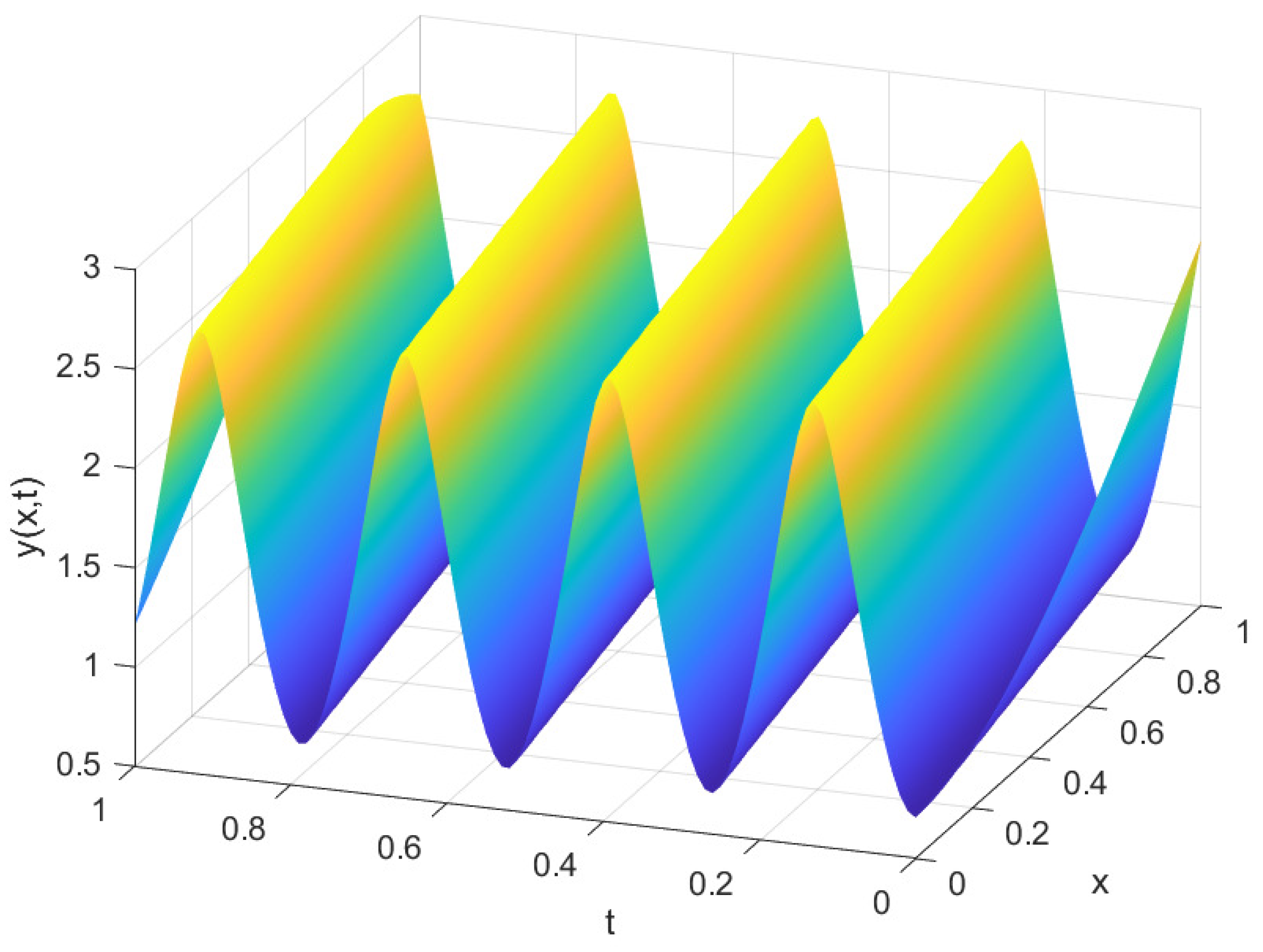
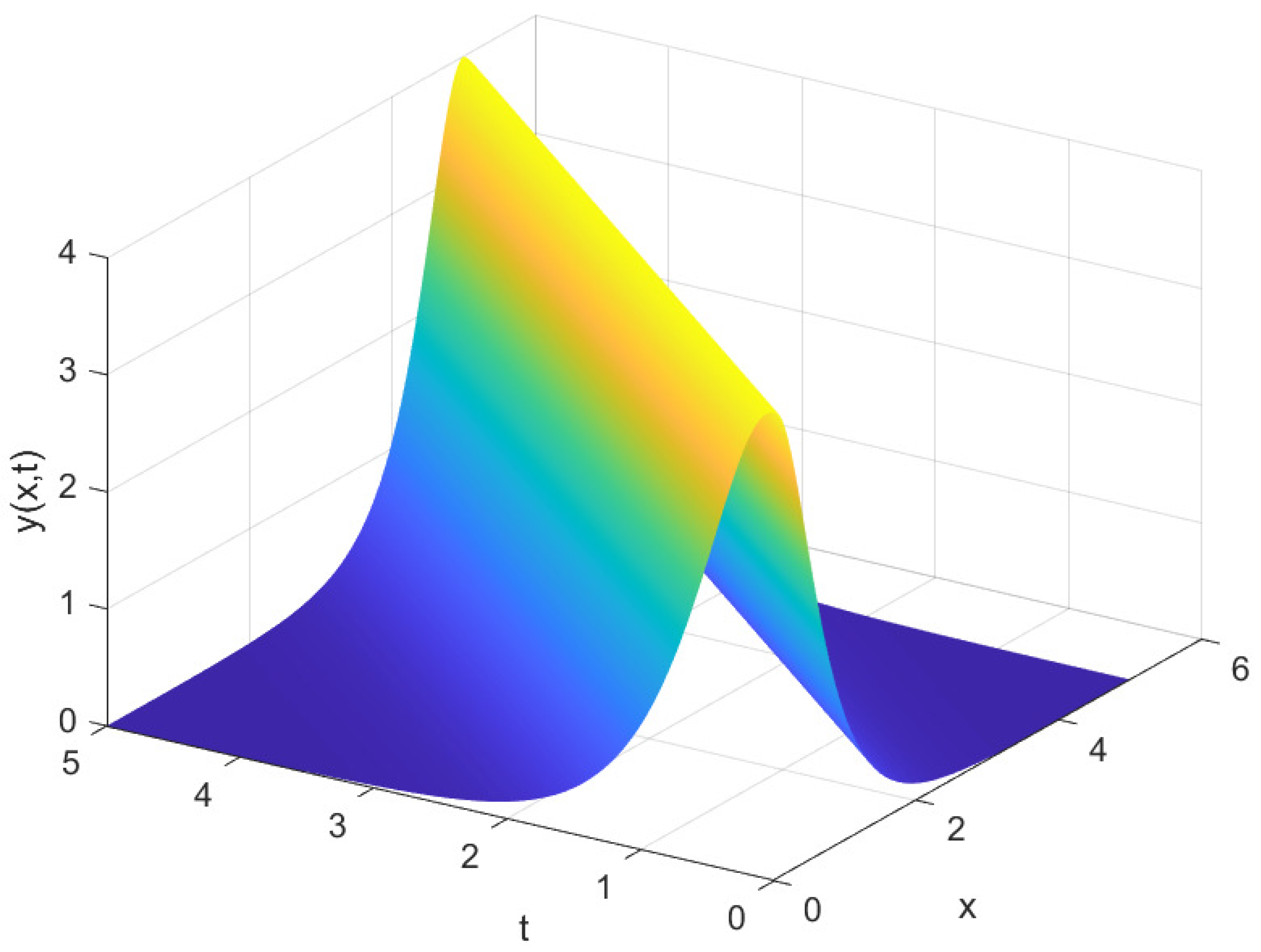
4. Periodic and Solitary Wave Solutions of the System of Ordinary Differential Equations Obtained

According to the values of the smallest powers of the solutions’ $y\left(z\right)$ and $\psi \left(z\right)$ expansions in the Puiseux series obtained during the course of the Painlevé test, we look for exact solutions according to the simplest equation algorithm (for examples of its applications and variations see, for instance, refs. [27,28,29,30,31]) in the following form:

$$\begin{array}{c}y\left(z\right)=\sqrt{V\left(z\right)},\psi \left(z\right)=p+\frac{r}{V\left(z\right)}+sV,\end{array}$$

(28)

where $V\left(z\right)$ is the solution of a simpler equation, which reads

$$\begin{array}{c}{V}_z^2=a{V}^4+b{V}^3+c{V}^2+dV+h,\end{array}$$

(29)

in which p, r, s, a, b, c, d, and h are unknown real parameters to be determined.

Substituting the ansatz (28) into Equations (7) and (8) and taking into account Equation (29) differentiated once and twice with respect to z,

$$\begin{array}{c}{V}_{zz}=2a{V}^3+\frac{3}{2}b{V}^2+cV+\frac{d}{2}\end{array}$$

(30)

and

$$\begin{array}{c}{V}_{zzz}=6a{V}^2{V}_z+3bV{V}_z+c{V}_z,\end{array}$$

(31)

yields a polynomial in a new unknown function $V\left(z\right)$. Equating coefficients at different powers of $V\left(z\right)$ to zero in the resulting equation, we obtain the following four parameter restrictions that can be realized for the system of Equations (7) and (8) to possess an exact solution

$$s_1=\frac{3}{4},a_1=-\frac{1}{4},b_1=0,c_1=-6r_1+4C_{0_1},h_1=-4r_1^2,p_1=0.$$

(32)

$$s_2=\frac{5}{8},a_2=-\frac{1}{16},b_2=0,c_2=-r_2,d_2=0,h_2=-4r_2^2,p_2=0,C_{0_2}=2r_2.$$

(33)

$$s_3=\frac{5}{4},a_3=-\frac{1}{4},b_3=0,c_3=-2r_3,d_3=0,h_3=-4r_3^2,p_3=0,C_{0_3}=-2r_3.$$

(34)

$$s_4=\frac{3}{4},a_4=-\frac{1}{4},b_4=-2p_4,c_4=-4p_4^2+2r_4,h_4=-4r_4^2,C_{0_4}=-4p_4^2+2r_4.$$

(35)

In Formulas (32)–(35), $s_i,a_i,b_i,c_i,d_i,h_i,p_i,C_{0_i},i=1..4$ are unknown parameters from the substitutions (28) and (29), where i corresponds to the number of parameter configurations in the partial exact solution.

We find that in the first partial case, $y_1\left(z\right)$ and ${\psi }_1\left(z\right)$ are determined by the solution of the following equation:

$$\begin{array}{c}{V}_z^2=-\frac{1}{4}{V}^4+(4C_{0_1}-6r_1)V^2+d_{1}V-4r_1^2,\end{array}$$

(36)

where $d_1$ and $r_1$ are arbitrary constants.

Accordingly, we have that $y_2\left(z\right)$ and ${\psi }_2\left(z\right)$ are expressed via the solution $V_2\left(z\right)$ of the differential equation, which reads

$$V_z^2=-\frac{1}{16}{V}^4-r_2{V}^2-4r_2^2=-{\left(\frac{1}{4}{V}^2+2r_2\right)}^2,$$

(37)

where $r_2$ is an arbitrary constant.

Substituting (34) into Equation (29) yields an ordinary differential equation for determining $y_3\left(z\right)$ and ${\psi }_3\left(z\right)$

$$V_z^2=-\frac{1}{4}{V}^4-2r_3{V}^2-4r_3^2=-{\left(\frac{1}{2}{V}^2+2r_3\right)}^2,$$

(38)

where $r_3$ is an arbitrary constant.

Finally, we obtain the following equation for finding the partial exact solutions $y_4\left(z\right)$ and ${\psi }_4\left(z\right)$ in the fourth case of parameter values (35):

$$V_z^2=-\frac{1}{4}{V}^4-2p_4{V}^3+(2r_4-4p_4^2)V^2+d_{4}V-4r_4^2,$$

(39)

where $r_4,d_4$, and $p_4$ are arbitrary constants.

Now, we solve the above equations. First, we rewrite Equation (36) as

$$V_z^2=-\frac{1}{4}(V-{\alpha }_1)(V-{\beta }_1)(V-{\gamma }_1)(V-{\delta }_1),$$

(40)

where ${\alpha }_1,{\beta }_1,{\gamma }_1,{\delta }_1$ are real roots of the following algebraic equation:

$$V^4-8(2C_{0_1}-3r_1)V^2-4d_{1}V+16r_1^2\equiv (V-{\alpha }_1)(V-{\beta }_1)(V-{\gamma }_1)(V-{\delta }_1)=0.$$

(41)

Making the following substitutions in Equation (40):

$$V\left(z\right)=\frac{{\beta }_1\left({\alpha }_1-{\delta }_1\right)v^2\left(z\right)+{\alpha }_1({\delta }_1-{\beta }_1)}{({\alpha }_1-{\delta }_1)v^2\left(z\right)+{\delta }_1-{\beta }_1},z^{\prime }={\chi }_{1}z,$$

(42)

where

$${\chi }_1=\frac{\sqrt{({\beta }_1-{\delta }_1)({\gamma }_1-{\alpha }_1)}}{4}$$

(43)

yields

$${\left(\frac{dv}{d{z}^{\prime }}\right)}^2=(1-v^2)(1-k_1^2{v}^2),$$

(44)

which is an equation for Jacobi elliptic sine with

$$k_1^2=\frac{({\alpha }_1-{\delta }_1)({\gamma }_1-{\beta }_1)}{({\beta }_1-{\delta }_1)({\gamma }_1-{\alpha }_1)}.$$

(45)

Consequently, the solution of Equation (36) reads

$$V_1\left(z\right)=\frac{{\beta }_1({\alpha }_1-{\delta }_1){\mathrm{sn}}^2({\chi }_1(z-z_1),k_1)+{\alpha }_1({\delta }_1-{\beta }_1)}{({\alpha }_1-{\delta }_1){\mathrm{sn}}^2({\chi }_1(z-z_1),k_1)+{\delta }_1-{\beta }_1},$$

(46)

where $z_1$ is a constant of integration.

Coming back to the original variables $y\left(z\right)$ and $\psi \left(z\right)$ yields the following exact solutions in the first case of parameter values (32):

$$y_1\left(z\right)={\left(\frac{{\beta }_1({\alpha }_1-{\delta }_1){\mathrm{sn}}^2({\chi }_1(z-z_1),k_1)+{\alpha }_1({\delta }_1-{\beta }_1)}{({\alpha }_1-{\delta }_1){\mathrm{sn}}^2({\chi }_1(z-z_1),k_1)+{\delta }_1-{\beta }_1}\right)}^{\frac{1}{2}},$$

(47)

and

$$\begin{array}{c}{\psi }_1\left(z\right)=\frac{r_1({\alpha }_1-{\delta }_1){\mathrm{sn}}^2({\chi }_1(z-z_1),k_1)+r_1({\delta }_1-{\beta }_1)}{{\beta }_1({\alpha }_1-{\delta }_1){\mathrm{sn}}^2({\chi }_1(z-z_1),k_1)+{\alpha }_1({\delta }_1-{\beta }_1)}+\\ \\ +\frac{3}{4}\frac{{\beta }_1({\alpha }_1-{\delta }_1){\mathrm{sn}}^2({\chi }_1(z-z_1),k_1)+{\alpha }_1({\delta }_1-{\beta }_1)}{({\alpha }_1-{\delta }_1){\mathrm{sn}}^2({\chi }_1(z-z_1),k_1)+{\delta }_1-{\beta }_1}.\end{array}$$

(48)

As we have previously made the substitution ${\varphi }_z=\psi$, the phase is expressed as ${\varphi }_1\left(z\right)=\int {\psi }_1\left(z\right)dz$. Unfortunately, this solution is too cumbersome to present here.

The solutions described by Equations (47) and (48) contain three arbitrary constants: $d_1,r_1$, and $z_1$. When two of the real roots of Equation (41) coincide, the solutions obtained can be reduced to solitary waves. Setting ${\gamma }_1={\delta }_1$ gives $k_1^2=1$, in which case, Jacobi elliptic sine is reduced in the following way:

$$\mathrm{sn}({\chi }_1(z-z_1),k_1)=tanh\left({\chi }_1(z-z_1)\right).$$

Therefore, the amplitude of the solitary wave solution reads

$$y_1^s\left(z\right)={\left(\frac{{\beta }_1({\alpha }_1-{\delta }_1){tanh}^2{\chi }_1(z-z_1)+{\alpha }_1({\delta }_1-{\beta }_1)}{({\alpha }_1-{\delta }_1){tanh}^2{\chi }_1(z-z_4)+{\delta }_1-{\beta }_1}\right)}^{\frac{1}{2}}.$$

(49)

and the phase (${\varphi }_1^s\left(z\right)=\int {\psi }_1^s\left(z\right)dz$) is expressed by the formula

$$\begin{array}{c}{\psi }_1^s\left(z\right)=p_1+\frac{r_1({\alpha }_1-{\delta }_1){tanh}^2{\chi }_1(z-z_1)+r_1({\delta }_1-{\beta }_1)}{{\beta }_1({\alpha }_1-{\delta }_1){tanh}^2{\chi }_1(z-z_1)+{\alpha }_1({\delta }_1-{\beta }_1)}+\\ +\frac{3}{4}\frac{{\beta }_1({\alpha }_1-{\delta }_1){tanh}^2{\chi }_1(z-z_1)+{\alpha }_1({\delta }_1-{\beta }_1)}{({\alpha }_1-{\delta }_1){tanh}^2{\chi }_1(z-z_1)+{\delta }_1-{\beta }_1}.\end{array}$$

(50)

In Equations (49) and (50), we have

$${\chi }_1=\frac{1}{4}\sqrt{({\beta }_1-{\delta }_1)({\delta }_1-{\alpha }_1)}.$$

(51)

Figure 1 and Figure 2 contain examples of plots of periodic and solitary wave solutions described by Equations (47) and (49).

In the second case of parameter values, Equation (37) can be easily integrated and has the solutions as follows:

$$V_2\left(z\right)=2\sqrt{-2r_2}tanh\left(\frac{\sqrt{2r_2}(z-z_2)}{2}\right),$$

(52)

where $z_2$ is an arbitrary constant. This solution cannot be used to describe solitary waves because it is a kink.

For the third case, Equation (38) is integrated in the same fashion as Equation (37) and has the solution expressed by the formula

$$V_3\left(z\right)=2\sqrt{-r_3}tanh\left(\sqrt{r_3}(z-z_3)\right),$$

(53)

where $z_3$ is an arbitrary constant. This solution also describes a kink.

Finally, we rewrite Equation (39) as

$$V_z^2=-\frac{1}{4}(V-{\alpha }_4)(V-{\beta }_4)(V-{\gamma }_4)(V-{\delta }_4),$$

(54)

where ${\alpha }_4,{\beta }_4,{\gamma }_4,{\delta }_4$ are real roots of the algebraic equation

$$V^4+8p_4{V}^3-4(2r_4-4p_4^2)V^2-4d_{4}V+16r_4^2\equiv (V-{\alpha }_4)(V-{\beta }_4)(V-{\gamma }_4)(V-{\delta }_4)=0.$$

(55)

Making the substitution in Equation (54) in the following way:

$$V\left(z\right)=\frac{{\beta }_4\left({\alpha }_4-{\delta }_4\right)v^2\left(z\right)+{\alpha }_4({\delta }_4-{\beta }_4)}{({\alpha }_4-{\delta }_4)v^2\left(z\right)+{\delta }_4-{\beta }_4},z^{\prime }={\chi }_{4}z,$$

(56)

where

$${\chi }_4=\frac{\sqrt{({\beta }_4-{\delta }_4)({\gamma }_4-{\alpha }_4)}}{4},$$

(57)

yields the following equation

$${\left(\frac{dv}{d{z}^{\prime }}\right)}^2=(1-v^2)(1-k_4^2{v}^2),$$

(58)

which has a general solution described by Jacobi elliptic sine $\mathrm{sn}({\chi }_4(z-z_4),k_4)$, where $k_4$ is defined as follows:

$$k_4^2=\frac{({\alpha }_4-{\delta }_4)({\gamma }_4-{\beta }_4)}{({\beta }_4-{\delta }_4)({\gamma }_4-{\alpha }_4)},$$

(59)

and where $z_4$ is an integration constant.

Consequently, the solution of Equation (36) in the fourth case reads

$$V_4\left(z\right)=\frac{{\beta }_4({\alpha }_4-{\delta }_4){\mathrm{sn}}^2({\chi }_4(z-z_4),k_4)+{\alpha }_4({\delta }_4-{\beta }_4)}{({\alpha }_4-{\delta }_4){\mathrm{sn}}^2({\chi }_4(z-z_4),k_4)+{\delta }_4-{\beta }_4}.$$

(60)

Returning to the original variables, we have

$$y_4\left(z\right)={\left(\frac{{\beta }_4({\alpha }_4-{\delta }_4){\mathrm{sn}}^2({\chi }_4(z-z_4),k_4)+{\alpha }_4({\delta }_4-{\beta }_4)}{({\alpha }_4-{\delta }_4){\mathrm{sn}}^2({\chi }_4(z-z_4),k_4)+{\delta }_4-{\beta }_4}\right)}^{\frac{1}{2}}$$

(61)

and

$$\begin{array}{c}{\psi }_4\left(z\right)=p_4+\frac{r_4({\alpha }_4-{\delta }_4){\mathrm{sn}}^2({\chi }_4(z-z_4),k_4)+r_4({\delta }_4-{\beta }_4)}{{\beta }_4({\alpha }_4-{\delta }_4){\mathrm{sn}}^2({\chi }_4(z-z_4),k_4)+{\alpha }_4({\delta }_4-{\beta }_4)}+\\ +\frac{3}{4}\left(\frac{{\beta }_4({\alpha }_4-{\delta }_4){\mathrm{sn}}^2({\chi }_4(z-z_4),k_4)+{\alpha }_4({\delta }_4-{\beta }_4)}{({\alpha }_4-{\delta }_4){\mathrm{sn}}^2({\chi }_4(z-z_4),k_4)+{\delta }_4-{\beta }_4}\right).\end{array}$$

(62)

As we have previously made the substitution ${\varphi }_z=\psi$, the phase is expressed as ${\varphi }_4\left(z\right)=\int {\psi }_4\left(z\right)dz$. Unfortunately, this solution is too cumbersome to present here.

The solutions defined by Equations (61) and (62) in the general case describe periodic waves and contain four arbitrary constants: $p_4,r_4,d_4$, and $z_4$. Provided that Equation (55) has two coinciding real roots, the solutions obtained can be reduced to solitary waves. Setting ${\gamma }_4={\delta }_4$ yields $k_4^2=1$, from which it follows that

$$\mathrm{sn}({\chi }_4(z-z_4),k_4)=tanh\left({\chi }_4(z-z_4)\right),$$

so the amplitude of the solitary wave solution is expressed as

$$y_4^s\left(z\right)={\left(\frac{{\beta }_4({\alpha }_4-{\delta }_4){tanh}^2{\chi }_4(z-z_4)+{\alpha }_4({\delta }_4-{\beta }_4)}{({\alpha }_4-{\delta }_4){tanh}^2{\chi }_4(z-z_4)+{\delta }_4-{\beta }_4}\right)}^{\frac{1}{2}}.$$

(63)

and its phase (${\varphi }_4^s\left(z\right)=\int {\psi }_4^s\left(z\right)dz$) is described by the formula

$$\begin{array}{c}{\psi }_4^s\left(z\right)=p_4+\frac{r_4({\alpha }_4-{\delta }_4){tanh}^2{\chi }_4(z-z_4)+r_4({\delta }_4-{\beta }_4)}{{\beta }_4({\alpha }_4-{\delta }_4){tanh}^2{\chi }_4(z-z_4)+{\alpha }_4({\delta }_4-{\beta }_4)}+\\ +\frac{3}{4}\frac{{\beta }_4({\alpha }_4-{\delta }_4){tanh}^2{\chi }_4(z-z_4)+{\alpha }_4({\delta }_4-{\beta }_4)}{({\alpha }_4-{\delta }_4){tanh}^2{\chi }_4(z-z_4)+{\delta }_4-{\beta }_4}.\end{array}$$

(64)

In Equations (63) and (64), we have

$${\chi }_4=\frac{1}{4}\sqrt{({\beta }_4-{\delta }_4)({\delta }_4-{\alpha }_4)}.$$

(65)

Thus, the amplitudes of the solitary waves of Equation (1) can be described by formulas (49) and (63), and the phases of the solitary waves can accordingly be described by Equations (50) and (64), provided that algebraic Equations (41) and (55) have two coinciding real roots, so their discriminants $D_1$ and $D_4$ are zero.

5. Conclusions

This paper has explored the analytical properties of the third-order partial differential equation from the Kaup–Newell hierarchy. In the second section, the studied equation, with the aid of traveling wave variables, was reduced to a system of two ordinary differential equations describing the amplitude and phase of the solution. In the third section, the Painlevé analysis was applied to obtain local solutions of the system in Puiseux series. The fourth section contained periodic and solitary wave solutions of the traveling reduction of the studied equation, obtained using the simplest equation method. The exact analytical results obtained in this paper could facilitate the investigation of higher-order flows of other integrable nonlinear dynamical systems and provide a theoretical basis for possible experimental studies and applications. Potentially, one could investigate higher-order equations from the hierarchy and compare their exact solutions to the solution of the third-order equation.

References

1. Jawad, A.J.A.M.; Al Azzawi, F.J.I.; Biswas, A.; Khan, S.; Zhou, Q.; Moshokoa, S.P.; Belic, M.R. Bright and singular optical solitons for Kaup–Newell equation with two fundamental integration norms. Optik 2019, 182, 594–597. [Google Scholar] [CrossRef]
2. Biswas, A.; Ekici, M.; Sonmezoglu, A.; Alqahtani, R.T. Sub-pico-second chirped optical solitons in mono-mode fibers with Kaup–Newell equation by extended trial function method. Optik 2018, 168, 208–216. [Google Scholar] [CrossRef]
3. Wang, K.L. Novel solitary wave and periodic solutions for the nonlinear Kaup–Newell equation in optical fibers. Opt. Quant. Electron. 2024, 56, 514. [Google Scholar] [CrossRef]
4. Salas, A.H.; El-Tantawy, S.A.; Youssef, A.A.A.R. New solutions for chirped optical solitons related to Kaup-Newell equation: Application to plasma physics. Optik 2020, 218, 165203. [Google Scholar] [CrossRef]
5. Yıldırım, Y.; Biswas, A.; Zhou, Q.; Alshomrani, A.S.; Belic, M.R. Sub pico-second optical pulses in birefringent fibers for Kaup–Newell equation with cutting-edge integration technologies. Results Phys. 2019, 15, 102660. [Google Scholar] [CrossRef]
6. Ahmed, H.M.; Rabie, W.B.; Ragusa, M.A. Optical solitons and other solutions to Kaup–Newell equation with Jacobi elliptic function expansion method. Anal. Mat. Phys. 2021, 11, 1–16. [Google Scholar] [CrossRef]
7. Zayed, E.M.; El-Horbaty, M.; Gepreel, K.A. Dispersive optical soliton solutions in birefringent fibers with stochastic Kaup–Newell equation having multiplicative white noise. Math. Method. Appl. Sci. 2024, 47, 352–370. [Google Scholar] [CrossRef]
8. Kaup, D.J.; Newell, A.C. An exact solution for a derivative Schrödinger equation. J. Math. Phys. 1979, 19, 798. [Google Scholar] [CrossRef]
9. Imai, K. Generalization of the Kaup-Newell inverse scattering formulation and Darboux transformation. J. Phys. Soc. Jpn. 1999, 68, 355–359. [Google Scholar] [CrossRef]
10. Ablowitz, M.J.; Kaup, D.J.; Newell, A.C.; Segur, H. The inverse scattering transform-Fourier analysis for nonlinear problems. Stud. Appl. Math 1974, 53, 249–315. [Google Scholar] [CrossRef]
11. Grosse, H. New solitons connected to the Dirac equation. Phys. Rep. 1986, 134, 297–304. [Google Scholar] [CrossRef]
12. Solli, D.R.; Ropers, C.; Koonath, P.; Jalali, B. Optical rogue waves. Nature 2007, 450, 1054–1057. [Google Scholar] [CrossRef]
13. He, J.; Wang, L.; Li, L.; Porsezian, K.; Erdélyi, R. Few-cycle optical rogue waves: Complex modified Korteweg–de Vries equation. Phys. Rev. E 2014, 89, 062917. [Google Scholar] [CrossRef]
14. Zhu, J.Y.; Chen, Y. A new form of general soliton solutions and multiple zeros solutions for a higher-order Kaup–Newell equation. J. Math. Phys. 2021, 62, 12. [Google Scholar] [CrossRef]
15. Lin, H.; He, J.; Wang, L.; Mihalache, D. Several categories of exact solutions of the third-order flow equation of the Kaup–Newell system. Nonlinear Dynam. 2020, 100, 2839–2858. [Google Scholar] [CrossRef]
16. Clarkson, P.A.; Cosgrove, C.M. Painleve analysis of the non-linear Schrodinger family of equations. J. Phys. A Math. Gen. 1987, 2, 2003. [Google Scholar] [CrossRef]
17. Lü, X.; Peng, M. Painlevé-integrability and explicit solutions of the general two-coupled nonlinear Schrödinger system in the optical fiber communications. Nonlinear Dynam. 2013, 73, 405–410. [Google Scholar] [CrossRef]
18. Kudryashov, N.A.; Safonova, D.V.; Biswas, A. Painlevé analysis and a solution to the traveling wave reduction of the Radhakrishnan—Kundu—Lakshmanan equation. Regul. Chaotic Dyn. 2019, 24, 607–614. [Google Scholar] [CrossRef]
19. Kudryashov, N.A.; Safonova, D.V. Painlevé analysis and traveling wave solutions of the fourth-order differential equation for pulse with non-local nonlinearity. Optik 2021, 227, 166019. [Google Scholar] [CrossRef]
20. Kudryashov, N.A.; Safonova, D.V. Nonautonomous first integrals and general solutions of the KdV-Burgers and mKdV-Burgers equations with the source. Math. Meth. Appl. Sci. 2019, 42, 4627–4636. [Google Scholar] [CrossRef]
21. Kudryashov, N.A. Painlevé analysis and exact solutions of the Korteweg–de Vries equation with a source. Appl. Math. Lett. 2015, 41, 41–45. [Google Scholar] [CrossRef]
22. Ablowitz, M.J.; Ramani, A.; Segur, H. A connection between nonlinear evolution equations and ordinary differential equations of P-type. I. J. Math Phys. 1980, 21, 715–721. [Google Scholar] [CrossRef]
23. Goriely, A. Integrability and Nonintegrability of Dynamical Systems; World Scientific: Singapore, 2001; Volume 19. [Google Scholar]
24. Tabor, M.; Weiss, J. Analytic structure of the Lorenz system. Phys. Rev. A 1981, 24, 2157. [Google Scholar] [CrossRef]
25. Rañada, A.F.; Ramani, A.; Dorizzi, B.; Grammaticos, B. The weak-Painlevé property as a criterion for the integrability of dynamical systems. J. Math. Phys. 1985, 26, 708–710. [Google Scholar] [CrossRef]
26. Ramani, A.; Dorizzi, B.; Grammaticos, B. Painlevé conjecture revisited. Phys. Rev. Lett. 1982, 49, 1539–1541. [Google Scholar] [CrossRef]
27. Kudryashov, N.A. Simplest equation method to look for exact solutions of nonlinear differential equations. Chaos. Soliton. Fract. 2005, 24, 1217–1231. [Google Scholar] [CrossRef]
28. Zayed, E.M.; Shohib, R.M. Optical solitons and other solutions to Biswas–Arshed equation using the extended simplest equation method. Optik 2019, 185, 626–635. [Google Scholar] [CrossRef]
29. Kudryashov, N.A. Method for finding highly dispersive optical solitons of nonlinear differential equations. Optik 2020, 206, 163550. [Google Scholar] [CrossRef]
30. Rasheed, N.M.; Al-Amr, M.O.; Az-Zo’bi, E.A.; Tashtoush, M.A.; Akinyemi, L. Stable optical solitons for the Higher-order Non-Kerr NLSE via the modified simple equation method. Mathematics 2021, 9, 1986. [Google Scholar] [CrossRef]
31. Jawad, A.J.A.M.; Petković, M.D.; Biswas, A. Modified simple equation method for nonlinear evolution equations. Appl. Math. Comput. 2010, 217, 869–877. [Google Scholar]
Figure 1. Plot of the periodic solution y ( x , t ) (49) at r 1 = 1 , d 1 = 1 , C 0 1 = 10 .
Mathematics 12 01632 g001
Figure 2. Plot of the solitary solution y ( x , t ) (49) at r 1 = 0 , d 1 = 0 , C 0 1 = 1 .
Mathematics 12 01632 g002
Disclaimer/Publisher’s Note: The statements, opinions and data contained in all publications are solely those of the individual author(s) and contributor(s) and not of MDPI and/or the editor(s). MDPI and/or the editor(s) disclaim responsibility for any injury to people or property resulting from any ideas, methods, instructions or products referred to in the content.