Chaotic Phenomena, Sensitivity Analysis, Bifurcation Analysis, and New Abundant Solitary Wave Structures of The Two Nonlinear Dynamical Models in Industrial Optimization

Abstract

In this research, we discussed the different chaotic phenomena, sensitivity analysis, and bifurcation analysis of the planer dynamical system by considering the Galilean transformation to the Lonngren wave equation (LWE) and the (2 + 1)-dimensional stochastic Nizhnik–Novikov–Veselov System (SNNVS). These two important equations have huge applications in the fields of modern physics, especially in the electric signal in data communication for LWE and the mechanical signal in a tunnel diode for SNNVS. A different chaotic nature with an additional perturbed term was also highlighted. Concerning the theory of the planer dynamical system, the bifurcation analysis incorporating phase portraits of the dynamical systems of the declared equations was performed. Additionally, a sensitivity analysis was used to monitor the sensitivity of the mentioned equations. Also, we extracted new, abundant solitary wave structures with the graphical phenomena of the mentioned nonlinear mathematical models. By conducting an expansion method on the abovementioned equations, we generated three types of soliton structures, which are rational function, trigonometric function, and hyperbolic function. By simulating the 3D, contour, and 2D graphs of these obtained solitons, we scrutinized the behavior of the waves affecting the nonlinear terms. The figures show that the solitary waves obtained from LWE are efficient in analyzing electromagnetic wave signals in the cable lines, and the solitary waves from SNNVS are essential in any stochastic system like a sound wave. Moreover, by taking some values of the parameters, we found some interesting soliton shapes, such as compaction soliton, singular periodic solution, bell-shaped soliton, anti-kink-shaped soliton, one-sided kink-shaped soliton, and some flat kink-shaped solitons, etc. This article will have a great impact on nonlinear science due to the new solitary wave structures with different complex phenomena, sensitivity analysis, and bifurcation analysis.

1. Introduction

Nonlinear partial differential equations (NPDEs) make an indispensable impact on giving the model for characterizing the complex natural occurrence of many scientific and engineering phenomena, namely, optical fibers, mechanics, plasma physics, reaction models, chemical kinematics, fluid dynamics, relativistic physics, biological science, and so on [1,2,3,4,5,6,7,8,9,10,11,12,13,14,15,16,17,18,19,20,21,22,23,24,25,26,27,28,29,30,31,32,33,34,35,36,37,38,39,40,41,42,43,44,45]. It is highly important to investigate the progressive wave-like solution for the best perception of NLPDEs and their application in real life. Lately, different kinds of techniques have been exhibited for generating numerical and analytical demonstrations by many experts, such as the Riccati equation method [1], the F-expansion technique [2,3], the auxiliary equation method [4,5], the Jacobi elliptic function method [6,7], the direct algebraic function technique [8,9], the Cole–Hopf conversion technique [10,11], the tanh-function method [12,13], the Backlund transform technique [14,15], the Hirota’s bilinear technique [16,17,18], the exp($-\varphi \left(\xi \right)$)-expansion method [19,20], the generalized Kudryashov method [21,22], the homotopy exploration technique [23], the homogeneous balance technique [24,25,26], the variational iteration method [27], the sine cosine algorithm [28], and the $\left(\frac{G^{\prime }}{G^{\prime }+G+A} \right)$-expansion technique [29,30,31]. In addition, the $\left(G^{\prime }/G\right)$-expansion technique was introduced by Wang et al. for describing the outcomes of NLPDEs [32]. Many investigators have applied this technique in their investigative works [33,34,35,36,37,38,39,40]. In addition to these, many investigators aspired to look for other alternatives that are more diligent and better than the former technique. Recently, Iqbal et al. [41] and Miah et al. [42] have applied the $\left(G^{\prime }/G,1/G\right)$-expansion technique to attain new soliton solutions for the mZK equation and the Gerdjikov–Ivanov equation and have applied the abundant closed-form wave solution to some NLEEs in mathematical physics, respectively. Moreover, many scientists [43,44,45,46,47,48] have chosen it as a mechanism to obtain the solution for NLPDEs. In this program, we detail and engage the $\left(G^{\prime }/G,1/G\right)$-expansion method to analyze the LWE and the (2 + 1)-dimensional SNNVS of the nonlinear electrical transmission line and the propagation of the stochastic systems, which have not been yet been tried with our method.

Lately, a great deal of research has been completed on nonlinear systems. Many disciplines, especially engineering, telecommunications, and ecology alongside economics, have explored bifurcation as well as chaotic nature, which is an appealing nonlinear phenomenon. We can better understand the process in which systems move from a stable state to an unstable state by having an in-depth knowledge of bifurcations. When the behavior of a dynamical system depends extensively on the initial condition, it is categorized as chaotic. Chaos theory, which has implications in ecology, weather forecasting, and financial markets, emphasizes the innate difficulty and variability of dynamic systems. Moreover, the Runge–Kutta technique is exercised for the sensitivity analysis of a dynamical system. The entire analysis provides insightful information on the suggested dynamical systems, which is amazing and useful for engineering and mathematical physics, as well as for developing a better comprehension of real-world occurrences and supporting control alongside anticipation.

The novelty of our research work is that our obtained results from the LWE, also known as the wave equation in general, can give the fundamental concept in physics and engineering that describes the behavior of waves. Also, our obtained solutions can be used in numerous applications across various fields, including acoustics; the attained solutions of the LWE can be used to study the propagation of sound waves in different mediums. This is crucial in designing acoustic systems in concert halls, auditoriums, and soundproofing materials. In seismology, seismologists can use these solutions to analyze seismic waves generated by earthquakes. This helps in understanding the Earth’s interior structure and predicting the impact of seismic events. In electromagnetics, our obtained results can be applied to describe the behavior of electromagnetic waves, including light, radio waves, and microwaves. Our results can also be used in designing antennas, optical fibers, and other communication systems. In engineering, engineers may use our results from the LWE to analyze and design structures subjected to dynamic loads, such as vibrations and oscillations. This is crucial in fields like civil engineering, mechanical engineering, and aerospace engineering. In medical imaging, techniques like ultrasound and MRI rely on the principles of wave propagation. Understanding the wave equation is essential in developing and interpreting the images produced by these medical imaging modalities. In oceanography, oceanographers may use the results to study ocean waves and currents, which are essential for understanding climate patterns, coastal erosion, and navigation safety. In quantum mechanics, the results can describe the behavior of quantum particles such as electrons and photons. This is fundamental for understanding the behavior of matter at the atomic and subatomic levels. In optics, these wave solutions are crucial for understanding phenomena like diffraction, interference, and the polarization of light. This understanding can be applied in designing optical instruments, lenses, and imaging systems. In material science, understanding how waves propagate through materials is crucial for studying properties like elasticity, conductivity, and thermal conductivity. This knowledge is applied in various industries, including construction, electronics, and aerospace. In geophysics, geophysicists can use our results to study various phenomena such as seismic exploration for oil and gas, groundwater mapping, and environmental monitoring.

These are just a few examples of how the obtained results can be applied in real-life scenarios across different disciplines. The equation’s versatility and fundamental nature make it a cornerstone of modern physics and engineering. The LWE is of the following form [49,50],

$${\left(u_{xx}-\alpha u+\beta u^2\right)}_{tt}+u_{xx}=0,$$

(1)

with two arbitrary constants $\alpha$ and $\beta$.

The (2 + 1)-dimensional SNNVS is a mathematical model that describes certain physical phenomena in a specific mathematical framework. Our obtained results from the SNNVS have potential applications in various fields of science and technology.

In nonlinear optics, the obtained solutions can be used to describe the behavior of optical solitons in certain nonlinear optical media. Understanding and controlling solitons are important for developing technologies such as optical communication systems and fiber optics. In plasma physics, the obtained solutions may have applications in modeling certain behaviors in plasma physics, such as wave propagation and turbulence in plasmas. This is relevant in fields like nuclear fusion research and astrophysics. In fluid dynamics, the equation and its results governing fluid flow often exhibit nonlinear behavior similar to that described by the SNNVS. Understanding such behavior is crucial in various engineering applications, including weather prediction, aerodynamics, and oceanography. The obtained solutions can be related to certain aspects of quantum field theory and integrable systems. While the direct applications in everyday life may not be obvious, advancements in theoretical physics can lead to technological breakthroughs in the future. In mathematical physics research, the study of our soliton solutions to the SNNVS contributes to theoretical developments in mathematical physics. While this may not have immediate practical applications, it advances our understanding of fundamental physical principles, which can eventually lead to technological innovations. In materials science, understanding the mathematical properties of our results can provide insights into the behavior of complex materials, such as ferroelectric or ferromagnetic materials, which have applications in electronic devices, sensors, and data storage. In biophysics, nonlinear dynamics play a role in modeling certain biological processes, such as the propagation of nerve impulses or the dynamics of biochemical reactions. Insights gained from studying nonlinear systems like the obtained solutions of SNNVS can contribute to understanding biological phenomena.

Overall, while the obtained solutions of (2 + 1)-dimensional SNNVS may not have direct applications in everyday life, they are a valuable mathematical model that contributes to our understanding of complex physical phenomena and has potential applications in various scientific and technological fields. Now, the (2 + 1)-dimensional SNNVS with the Ito sense of augmentative noise [51,52] is as follows:

$$u_t+k{u}_{xxx}+r{u}_{yyy}+s{u}_x+q{u}_y-3k{\left(uv\right)}_x-3r{\left(uw\right)}_y+\sigma u{\beta }_t=0,$$

(2)

$$u_x=v_y, u_y=w_x$$

(3)

This paper has been arranged in this fashion: In Section 1, we give a brief introduction. We narrate the expansion method in Section 2. In Section 3, the applications of the LWE for chaotic, sensitivity, bifurcation, and soliton solutions are introduced. In Section 4, the applications of the SNNVS for chaotic, sensitivity, bifurcation, and soliton solutions are introduced. We give the graphical declaration in Section 5. In Section 6, we give the conclusion of this article.

2. Exposition of the Mentioned Method

Here, we give an exploration of the $\left(G^{\prime }/G,1/G\right)$-expansion method for tracing the actual results of two given convective equations. We take into consideration an ordinary differential equation (ODE) given below,

$$G^{″\left(\tau \right)}+\lambda G\left(\tau \right)=l,$$

(4)

and consider

$$Q=G^{\prime }/G,R=1/G.$$

(5)

In the above two equations, we set two connections between $Q$ and $R$ as

$$Q^{\prime }=-Q^2+lR-\lambda ,R^{\prime }=-QR.$$

(6)

Depending on $\lambda$ (positive, negative, or zero), Equation (4) provides us with the three types of results below,

Category 1.

For  $\lambda >0,$ we write the result of Equation (4) as [41,42,43,44,45,46,47,48],

$$G\left(\tau \right)=c_1\mathit{sin}\left(\sqrt{\lambda }\tau \right)+c_2\mathit{cos}\left(\sqrt{\lambda }\tau \right)+\frac{l}{\lambda },$$

(7)

and hence,

$$R^2=\frac{\lambda \left(Q^2-2lR+\lambda \right)}{{\lambda }^2\gamma -l^2},$$

(8)

where  $\gamma ={c_1}^2+{c_2}^2$.

Category 2.

For  $\lambda <0,$ the result of Equation (4) as [41,42,43,44,45,46,47,48],

$$G\left(\tau \right)=c_1\mathit{sin}h\left(\sqrt{-\lambda }\tau \right)+c_2\mathit{cos}h\left(\sqrt{-\lambda }\tau \right)+\frac{l}{\lambda },$$

(9)

and hence,

$$R^2=\frac{-\lambda \left(Q^2-2lR+\lambda \right)}{{\lambda }^2\delta +l^2},$$

(10)

where  $\delta ={c_1}^2-{c_2}^2$.

Category 3.

For  $\lambda =0$, the result of Equation (4) [41,42,43,44,45,46,47,48],

$$G\left(\tau \right)=\frac{l}{2}{\tau }^2+c_1\tau +c_2,$$

(11)

and

$$R^2=\frac{\left(Q^2-2lR\right)}{c_1^2-2l{c}_2}.$$

(12)

We suppose that an NLPDE of polynomial $P$ in $u\left(x,y,t\right)$ with some orders is given in the following way,

$$P\left(u,u_x,u_y,u_t,u_{xx},{u_{yy},u_{tt},u}_{xy},u_{xt},u_{yt}...\right)=0.$$

(13)

Thereafter, the details of the $\left(G^{\prime }/G,1/G\right)$-expansion method are the following steps:

Step 1. Applying the traditional transformation process, we write $u$ as a function of one variable,

$$u\left(x,y,t\right)=u\left(\tau \right), \tau =mx+ny-pt,$$

(14)

where $m$, $n$, $p$ are nonzero constants. Next, the corresponding ODE of Equation (13) is

$$O\left(u,-p{u}^{\prime },m{u}^{\prime },n{u}^{\prime },u^{″},u^{″},\dots \right)=0,$$

(15)

where polynomial $O$ is in $u\left(\tau \right)$ and its various order derivatives concerning $\tau$.

Step 2. We write a solution in Equation (15) in the function of $Q\left(\tau \right)$ and $R\left(\tau \right)$ as the following,

$$u\left(\tau \right)={\sum }_{m=0}^T{a}_m{Q}^m+{\sum }_{m=1}^T{b}_m{Q}^{m-1}R,$$

(16)

and the parameters $a_m\left(m=0, 1, 2,\dots ,T\right)$, $b_m\left(m=1, 2,\dots ,T\right), c,\lambda ,$ and $l$ will be gained through step 3. The balance number is obtained by applying the homogenous balance rules between the heights power nonlinear term and the heights differential term. In Equation (16), we put the obtained balance number, and after inserting it in Equation (15) and then using Equations (6), (8), (10), and (12), we change the left part of Equation (15) in $Q \mathrm{and} R,$ where the degree of Q is not greater than one and take it from zero up to any integral value.

Step 3. By equating the same index of the expression from the two parts, we obtain a pattern of algebraic solutions in $a_{m,} b_m, c,\lambda ,l,c_1, \mathrm{and} c_2$. Now, using computational software (we use Mathematica 13.1), we gain the results of obtaining an algebraic system. By putting the obtained results in Equation (16), we attain the outcomes of Equation (15). Now, by setting $\tau =\left(mx+ny-pt\right)$ in the outcomes of Equation (15), we attain the results of Equation (13). For more details of the mentioned method, visit [41,42,43,44,45,46,47,48].

3. Application of the LWE

In this section, the $\left(G^{\prime }/G,1/G\right)$-expansion method is engaged to extract the wave soliton solutions and to consider the following transformation,

$$u\left(x,t\right)=u\left(\tau \right) \mathrm{and} \tau =x-ct,$$

(17)

where $‘c’$ implies the wave velocity. Applying this transformation, we convert the LWE presented in Equation (1) to the following ODE,

$$c^2{u}^{″}+\left(1-c^2\alpha \right)u+c^2\beta u^2=0;$$

(18)

the prime implicates the derivative regarding $\tau$.

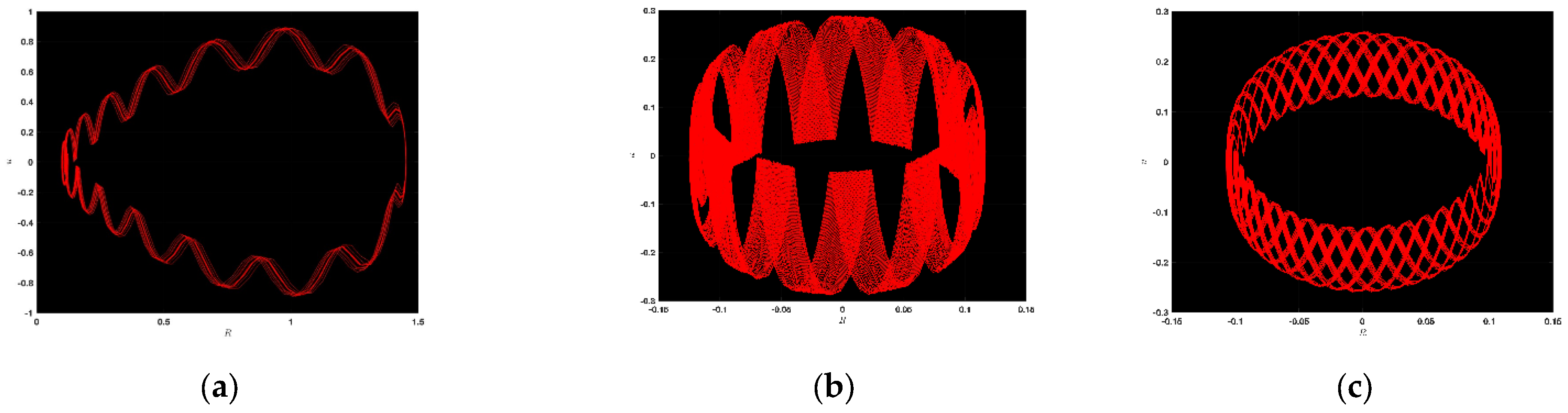
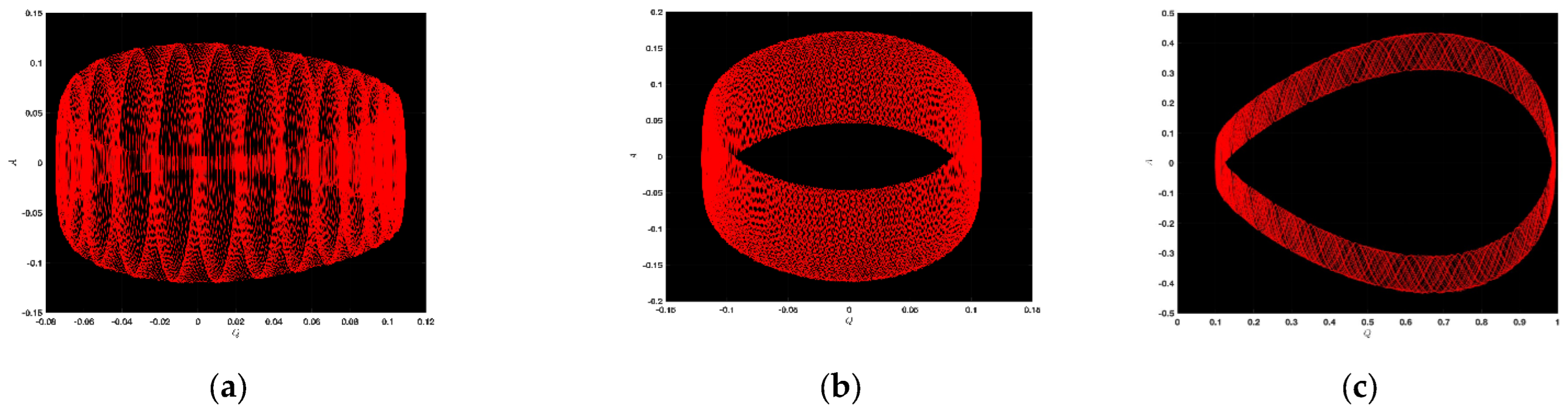
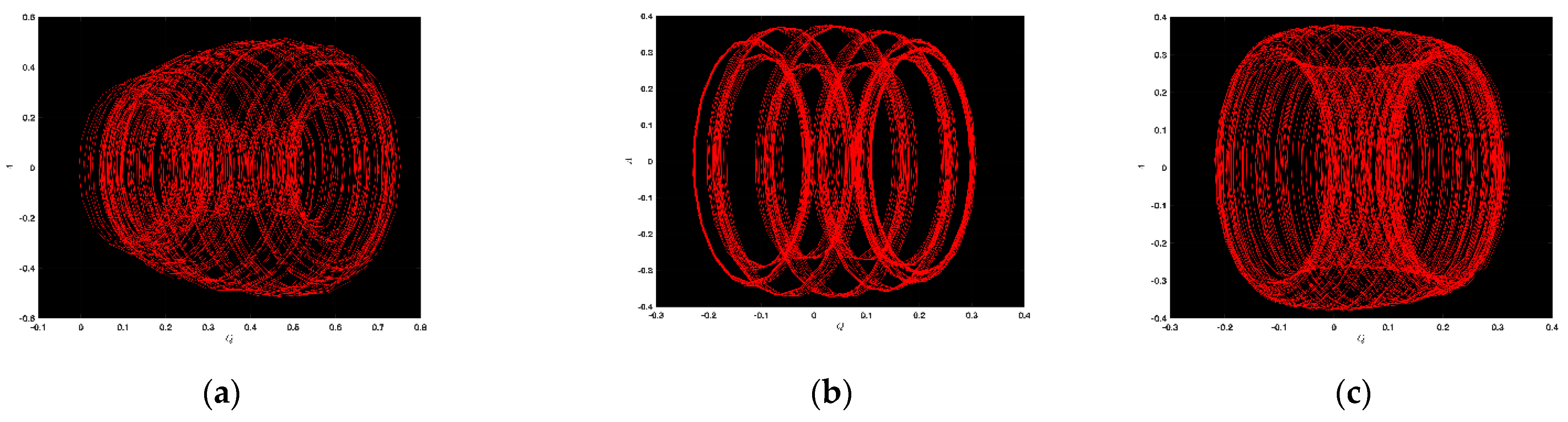
3.1. Chaotic Analysis of LWE

Here, we adapt Equation (18) within the planer dynamical system by considering the Galilean transformation [53,54,55,56],

$$\left\{\begin{array}{c}\frac{du\left(\tau \right)}{d\tau }=R \\ \frac{dR\left(\tau \right)}{d\tau }=W_1{u}^2\left(\tau \right)+W_{2}u\left(\tau \right) \end{array},\right.$$

(19)

in which $W_1=-\beta , W_2=\frac{c^2\alpha -1}{c^2}$. The perturbation term ${\zeta }_1\mathit{cos}\left({\zeta }_{2}t\right)$, where ${\zeta }_1$ stands for amplitude and ${\zeta }_2$ stands for the frequency, is introduced in the dynamical system of Equation (19) so that we can understand the chaotic character of the announced equation,

$$\left\{\begin{array}{l}\frac{du\left(t\right)}{dt}=R \\ \frac{dR\left(t\right)}{dt}=W_1{u}^2\left(t\right)+W_{2}u\left(t\right)+{\zeta }_1\mathit{cos}\left({\zeta }_{2}t\right) \end{array}.\right.$$

(20)

In this instance, the chaotic character of the above dynamical system is graphed for many specific values of the parameters. In Figure 1a, $\alpha =2, \beta =2, c=4, {\zeta }_1=2, \mathrm{and} {\zeta }_2=\pi /2$; in Figure 1b, $\alpha =-2, \beta =2, c=4, {\zeta }_1=2, \mathrm{and} {\zeta }_2=\pi /2$; in Figure 1c, $\alpha =0.5, \beta =-1, c=0.5, {\zeta }_1=1, \mathrm{and} {\zeta }_2=\pi /2$; in Figure 2a, $\alpha =2, \beta =2, c=1, {\zeta }_1=2, \mathrm{and} {\zeta }_2=\pi$; in Figure 2b, $\alpha =-3, \beta =-2, c=1, {\zeta }_1=1, \mathrm{and} {\zeta }_2=\pi$; in Figure 2c, $\alpha =-1, \beta =1, c=1, {\zeta }_1=1, \mathrm{and} {\zeta }_2=\pi$; in Figure 3a, $\alpha =1, \beta =1, c=2, {\zeta }_1=1, \mathrm{and} {\zeta }_2=2\pi$; in Figure 3b, $\alpha =-3, \beta =-2, c=2, {\zeta }_1=1, \mathrm{and} {\zeta }_2=2\pi$; and in Figure 3c, $\alpha =-3, \beta =2, c=2, {\zeta }_1=1, \mathrm{and} {\zeta }_2=2\pi$. In Figure 1a,b, we find out complex dynamics, and in Figure 1c, we have the limit cycle. In Figure 2a, we observe ringlet dynamics alongside Figure 2b as well as Figure 2c, which also depict strange dynamics. In addition, the limit cycle is displayed in Figure 3a; likewise, ringlet dynamics are also displayed in Figure 3b,c. Some strong and clear chaotic phenomena are designed that may be advantageous in mathematical physics and modern engineering.

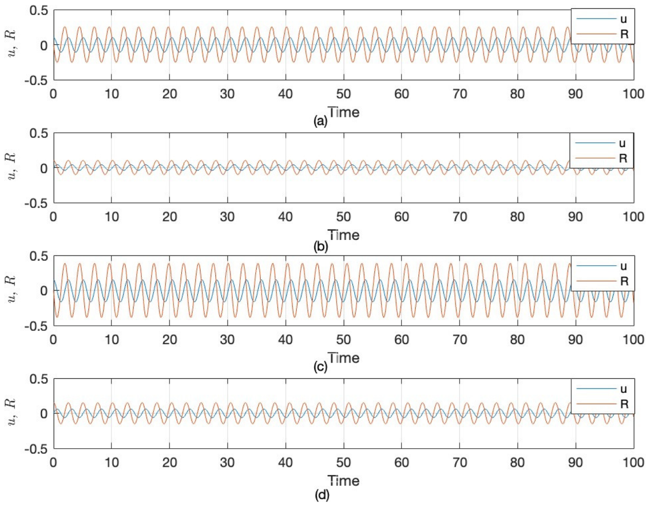
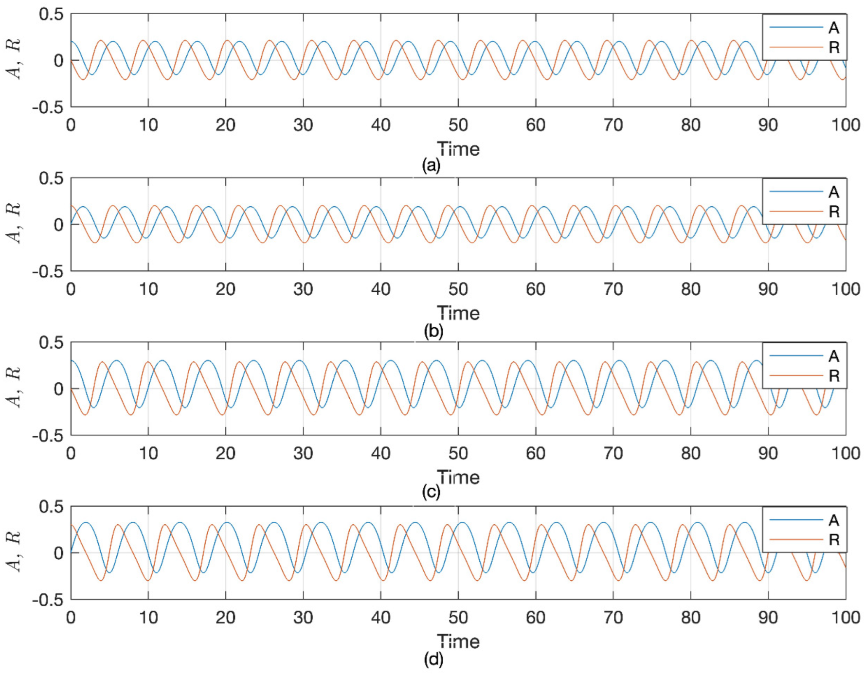
3.2. Sensitivity Analysis of LWE

In this subsection, our aim is to observe the sensitivity nature of the dynamic system stated in Equation (19). To complete this activity, we resolve the ensuing dynamical system in Equation (19) with the aid of the Runge–Kutta technique. The particular values of the parameters $\alpha =5, \beta =5, \mathrm{and} c=0.3$ are picked up for this instance. Furthermore, we assume the initial condition of the dynamical system as follows [53,54,55,56]:

(i)

$u\left(0\right)=0.1$ and $R=0$;

(ii)

$u\left(0\right)=0$ and $R=0.1$;

(iii)

$u\left(0\right)=0.15$ and $R=0$;

(iv)

$u\left(0\right)=0$ and $R=0.15$

The outcome is illustrated in Figure 4 for the abovementioned initial conditions, in which the blue curve represents the dynamics of class $u,$ and the orange curve signifies the dynamics of class $R$. It is demonstrated in Figure 4 that small alterations to the initial states have a major impact on the dynamical system.

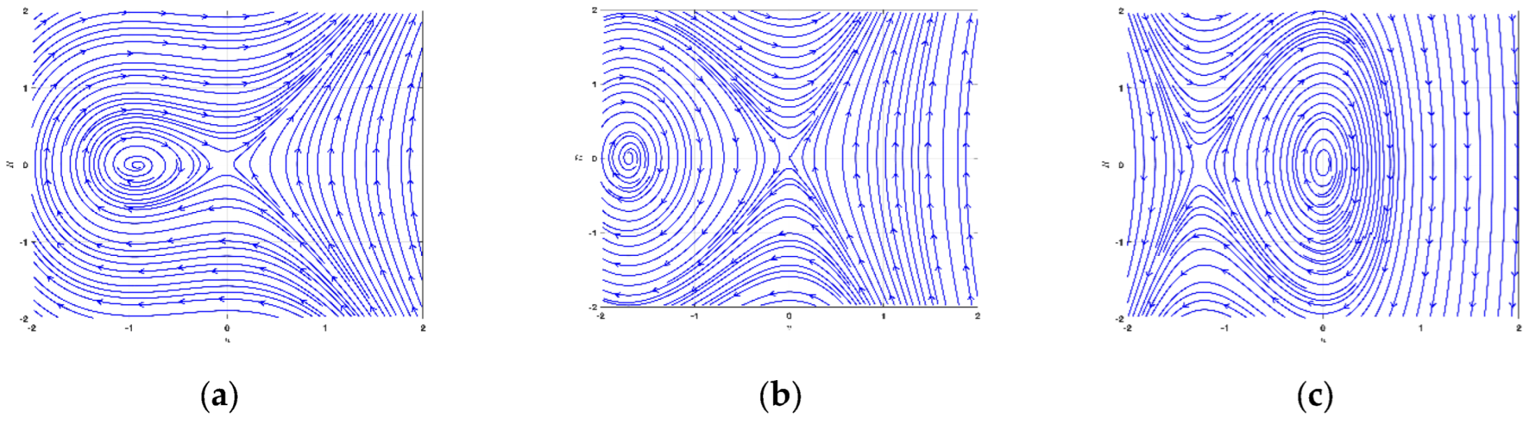
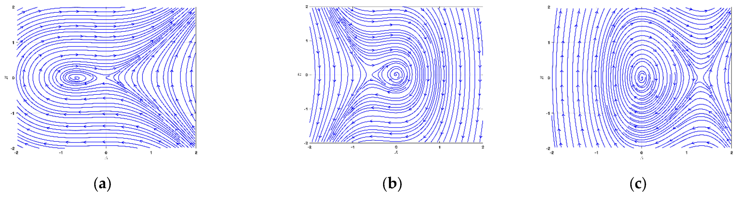
3.3. Bifurcation and Phase Portrait Analysis of LWE

The planer dynamical system in Equation (19) yields the subsequent Hamiltonian function as follows [53,54,55,56]:

$${\mathcal{H}}_1\left(u, R\right)=\frac{R^2}{2}-\frac{W_1{u}^3}{3}-\frac{W_2{u}^2}{2}={\mathcal{k}}_1.$$

Here, the Hamiltonian constant is represented by ${\mathcal{k}}_1$. We have the equilibrium positions at $\left(0, 0\right)$ and $\left(-\frac{W_2}{W_1}, 0\right),$ and we subsequently solve the next system,

$$\left\{\begin{array}{l}R=0 \\ {W_{1}u}^2+W_{2}u=0\end{array}.\right.$$

One can evaluate the Jacobian of the dynamical system in Equation (19):

$${\mathcal{D}}_1\left(u, R\right)=\left|\begin{array}{cc}0& 1\\ 2W_{1}u+W_2& 0\end{array}\right|=-2W_{1}u-W_2.$$

From the Planar dynamical systems theory, we have the following circumstances [53,54,55,56]:

• The equilibrium position $\left(u, R\right)$ denotes a saddle point, whereas ${\mathcal{D}}_1\left(u, R\right)<0$;
• The equilibrium position $\left(u, R\right)$ stands for a center point, whereas ${\mathcal{D}}_1\left(u, R\right)>0$;
• The equilibrium position $\left(u, R\right)$ characterizes a cuspid point, whereas ${\mathcal{D}}_1\left(u, R\right)=0$.

In the succeeding part, we obtain many situations that are discussed in depth for various conceivable parameter selections.

Instance 1: $W_1>0$ and $W_2>0$.

In Figure 5a, the equilibrium position $\left(0, 0\right)$ implies a saddle point that, together with the equilibrium position $\left(-0.9375, 0\right),$ implies a center point by selecting the parameters $\alpha =1, \beta =-1, \mathrm{and} c=4$.

Instance 2: $W_1>0$ and $W_2>0$

In Figure 5b, the equilibrium position $\left(0, 0\right)$ signifies a saddle point alongside the equilibrium position $\left(-1.7188, 0\right),$ which signifies a center point upon choosing the value of the parameters $\alpha =5, \beta =-2, \mathrm{and} c=0.8$.

Instance 3: $W_1<0$ and $W_2<0$

In Figure 5c, the equilibrium position $\left(0, 0\right)$ expresses a center point, and the equilibrium position $\left(-1.2222, 0\right)$ expresses a saddle point for the value of the parameters $\alpha =5, \beta =5, \mathrm{and} c=0.3$.

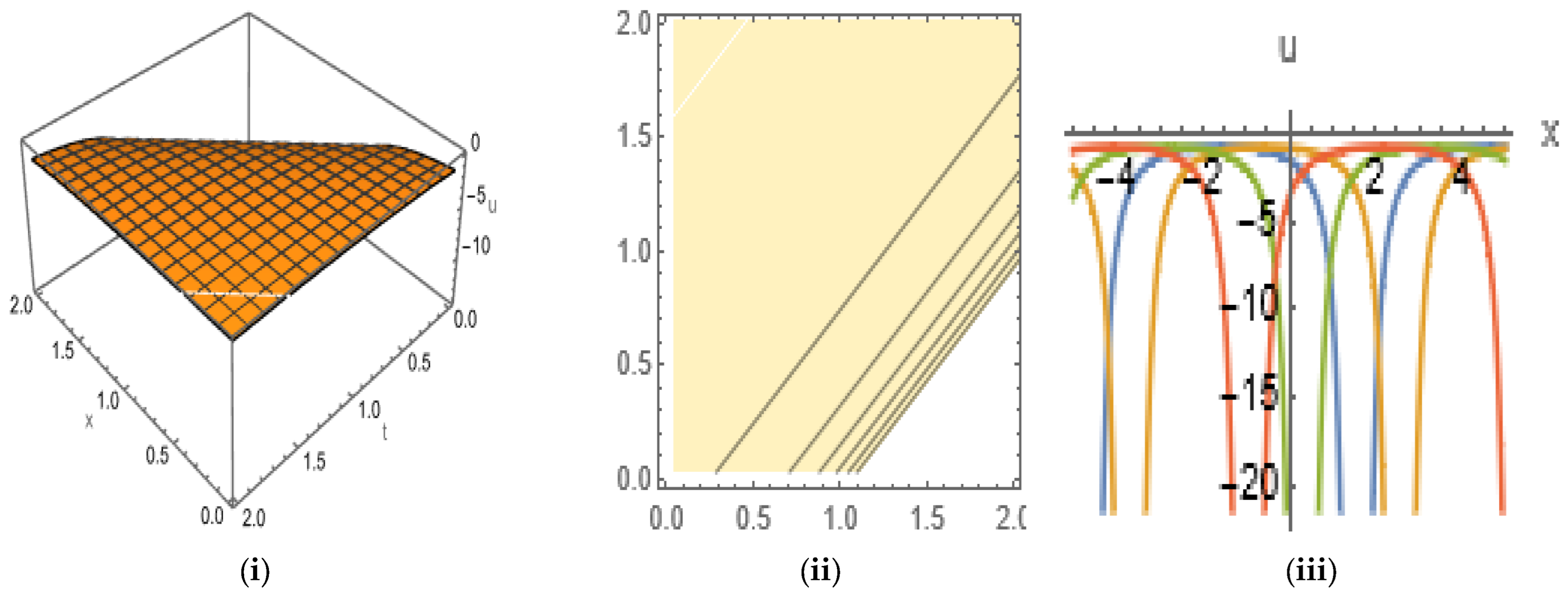
3.4. Soliton Solutions of LWE

In Equation (18), we apply the balance rule and obtain the balance number $T=2$. After placing this in Equation (16), we obtain

$$u\left(\tau \right)=a_0+a_{1}Q\left(\tau \right)+a_2{Q}^2\left(\tau \right)+b_{1}R\left(\tau \right)+b_{2}Q\left(\tau \right)R\left(\tau \right),$$

(21)

where the functions $Q\left(\tau \right)$ and $R\left(\tau \right)$ are stated in Equations (5) and (6). According to the signs of $\lambda$, the three kinds of basic outcomes of Equation (18) are as follows:

Case-1. For $\lambda >0$.

By taking two times differentiation of Equation (21) and utilizing Equations (6) and (8), we change the back side of Equation (21) in the variables of $Q$ and $R$. Now, by equating the constants of the coefficients in the gained polynomials to zero, we attain an algebraic system for the constants $a_0$, $a_1$, $a_2$, $b_1$, $b_2$, $\lambda ,$ and $c$. Lastly, by completing the procedure and applying the program Mathematica, we obtain two pairs of constants:

Set I:

$$a_0=\frac{-3\left(1-{\alpha c}^2\right)}{\beta c^2}, a_1=0, a_2=\frac{-3}{\beta }, b_1=\frac{3l}{\beta },$$

$$b_2=\pm \frac{3\sqrt{c^4{\alpha }^2\gamma -2c^2\alpha \gamma +\gamma -c^4{l}^2}}{\beta c\sqrt{1-\alpha c^2}} \mathrm{and} \lambda =\frac{1-\alpha c^2}{c^2};\alpha <\frac{1}{c^2}.$$

(22)

Set II:

$$a_0=\frac{-2\left(\alpha c^2-1\right)}{c^2\beta }, a_1=0, a_2=\frac{-3}{\beta }, b_1=\frac{3l}{\beta },$$

$$b_2=\pm \frac{3\sqrt{c^4{\alpha }^2\gamma -2c^2\alpha \gamma +\gamma -c^4{l}^2}}{\beta c\sqrt{\alpha c^2-1}} \mathrm{and} \lambda =\frac{\alpha c^2-1}{c^2} ; \alpha >\frac{1}{c^2}.$$

(23)

Now, after inserting the above set of values into Equation (21), we acquire the outputs of Equation (18). First, for set I,

$$\begin{array}{l}u\left(\tau \right)=\frac{-3\left(1-{\alpha c}^2\right)}{\beta c^2}-\frac{3\lambda }{\beta }{\left[\frac{c_1\mathit{cos}\left(\sqrt{\lambda }\tau \right)-c_2\mathit{sin}\left(\sqrt{\lambda }\tau \right)}{c_1\mathit{sin}\left(\sqrt{\lambda }\tau \right)+c_2\mathit{cos}\left(\sqrt{\lambda }\tau \right)+\frac{l}{\lambda }}\right]}^2+\frac{3l}{\beta }\frac{1}{\left[c_1\mathit{sin}\left(\sqrt{\lambda }\tau \right)+c_2\mathit{cos}\left(\sqrt{\lambda }\tau \right)+\frac{l}{\lambda }\right]}\pm \\ \frac{3\sqrt{\lambda }\sqrt{c^4{\alpha }^2\gamma -2c^2\alpha \gamma +\gamma -c^4{l}^2}}{\beta c\sqrt{1-\alpha c^2}}\frac{\left[c_1\mathit{cos}\left(\sqrt{\lambda }\tau \right)-c_2\mathit{sin}\left(\sqrt{\lambda }\tau \right)\right]}{{\left[c_1\mathit{sin}\left(\sqrt{\lambda }\tau \right)+c_2\mathit{cos}\left(\sqrt{\lambda }\tau \right)+\frac{l}{\lambda }\right]}^2},\end{array}$$

(24)

where $\lambda =\frac{1-\alpha c^2}{c^2}$ and $\alpha <\frac{1}{c^2}$. Now, taking $c_1=0$ and $l=0$ but $c_2\ne 0$ and inserting $\lambda =\frac{1-\alpha c^2}{c^2}$, $\tau =x-ct$ in Equation (24),

$$u\left(x,t\right)=\frac{-3\left(1-{\alpha c}^2\right)}{\beta c^2}\left[{\mathit{sec}}^2\{\sqrt{1-{\alpha c}^2}\left(\frac{x}{c}-t\right)\}\pm \mathit{tan}\{\sqrt{1-{\alpha c}^2}\left(\frac{x}{c}-t\right)\}\mathit{sec}\{\sqrt{1-{\alpha c}^2}\left(\frac{x}{c}-t\right)\}\right].$$

(25)

Again, when choosing $c_2=0$ and $l=0$ but $c_1\ne 0$,

$$u\left(x,t\right)=\frac{-3\left(1-{\alpha c}^2\right)}{\beta c^2}\left[{\mathit{cosec}}^2\{\sqrt{1-{\alpha c}^2}\left(\frac{x}{c}-t\right)\}\pm \mathit{cot}\{\sqrt{1-{\alpha c}^2}\left(\frac{x}{c}-t\right)\}\mathit{cosec}\{\sqrt{1-{\alpha c}^2}\left(\frac{x}{c}-t\right)\}\right]$$

(26)

where $\alpha <\frac{1}{c^2}$. For set II,

$$\begin{array}{l}u\left(\tau \right)=\frac{-2\left(\alpha c^2-1\right)}{\beta c^2}-\frac{3\lambda }{\beta }{\left[\frac{c_1\mathit{cos}\left(\sqrt{\lambda }\tau \right)-c_2\mathit{sin}\left(\sqrt{\lambda }\tau \right)}{c_1\mathit{sin}\left(\sqrt{\lambda }\tau \right)+c_2\mathit{cos}\left(\sqrt{\lambda }\tau \right)+\frac{l}{\lambda }}\right]}^2+\frac{3l}{\beta }\frac{1}{\left[c_1\mathit{sin}\left(\sqrt{\lambda }\tau \right)+c_2\mathit{cos}\left(\sqrt{\lambda }\tau \right)+\frac{l}{\lambda }\right]}\pm \\ \frac{3\sqrt{\lambda }\sqrt{c^4{\alpha }^2\gamma -2c^2\alpha \gamma +\gamma -c^4{l}^2}}{\beta c\sqrt{\alpha c^2-1}}\frac{\left[c_1\mathit{cos}\left(\sqrt{\lambda }\tau \right)-c_2\mathit{sin}\left(\sqrt{\lambda }\tau \right)\right]}{{\left[c_1\mathit{sin}\left(\sqrt{\lambda }\tau \right)+c_2\mathit{cos}\left(\sqrt{\lambda }\tau \right)+\frac{l}{\lambda }\right]}^2},\end{array}$$

(27)

where $\lambda =\frac{\alpha c^2-1}{c^2}$ and $\alpha >\frac{1}{c^2}$. By taking $c_1=0$ and $l=0$ but $c_2\ne 0$,

$$\begin{gathered} \left(x,t\right)=\frac{-2\left(\alpha c^2-1\right)}{\beta c^2}-\frac{3\left(\alpha c^2-1\right)}{\beta c^2} \\ \mathit{tan}\{\sqrt{\alpha c^2-1}\left(\frac{x}{c}-t\right)\}\mathit{sec}\{\sqrt{\alpha c^2-1}\left(\frac{x}{c}-t\right)\}, \end{gathered}$$

(28)

where $\alpha >\frac{1}{c^2}$. When choosing $c_2=0$ and $l=0$ but $c_1\ne 0$,

$$\begin{gathered} u\left(x,t\right)=\frac{-2\left(\alpha c^2-1\right)}{\beta c^2}-\frac{3\left(\alpha c^2-1\right)}{\beta c^2} \\ \mathit{cot}\{\sqrt{\alpha c^2-1}\left(\frac{x}{c}-t\right)\}\mathit{cosec}\{\sqrt{\alpha c^2-1}\left(\frac{x}{c}-t\right)\}, \end{gathered}$$

(29)

where $\alpha >\frac{1}{c^2}$.

Case-2. For $\lambda <0$, similarly to case-1, other two sets of solutions have been found as follows:

Set I:

$$\begin{gathered} a_0=\frac{3\left({\alpha c}^2-1\right)}{c^2\beta }, a_1=0, a_2=\frac{-3}{\beta }, b_1=\frac{3l}{\beta }, \\ b_2=\pm \frac{3\sqrt{c^4{\alpha }^2\delta -2c^2\alpha \delta +\delta -c^4{l}^2}}{\beta c\sqrt{\alpha c^2-1}} \mathrm{and} \lambda =\frac{1-\alpha c^2}{c^2};\alpha >\frac{1}{c^2}. \end{gathered}$$

(30)

Set II:

$$\begin{gathered} a_0=\frac{2\left(1-\alpha c^2\right)}{c^2\beta }, a_1=0, a_2=\frac{-3}{\beta }, b_1=\frac{3l}{\beta }, \\ b_2=\pm \frac{3\sqrt{c^4{\alpha }^2\delta -2c^2\alpha \delta +\delta -c^4{l}^2}}{\beta c\sqrt{1-\alpha c^2}} \mathrm{and} \lambda =\frac{\alpha c^2-1}{c^2} ; \alpha <\frac{1}{c^2}. \end{gathered}$$

(31)

Similarly, for Set I,

$$\begin{array}{l}u\left(\tau \right)=\frac{3\left({\alpha c}^2-1\right)}{\beta c^2}+\frac{3\lambda }{\beta }{\left[\frac{c_1\mathit{cos}h\left(\sqrt{-\lambda }\tau \right)-c_2\mathit{sin}h\left(\sqrt{-\lambda }\tau \right)}{c_1\mathit{sin}h\left(\sqrt{-\lambda }\tau \right)+c_2\mathit{cos}h\left(\sqrt{-\lambda }\tau \right)+\frac{l}{\lambda }}\right]}^2+\frac{3l}{\beta }\frac{1}{\left[c_1\mathit{sin}h\left(\sqrt{-\lambda }\tau \right)+c_2\mathit{cos}h\left(\sqrt{-\lambda }\tau \right)+\frac{l}{\lambda }\right]}\pm \\ \frac{3\sqrt{-\lambda }\sqrt{c^4{\alpha }^2\delta -2c^2\alpha \delta +\delta -c^4{l}^2}}{\beta c\sqrt{\alpha c^2-1}}\frac{\left[c_1\mathit{cos}h\left(\sqrt{-\lambda }\tau \right)-c_2\mathit{sin}h\left(\sqrt{-\lambda }\tau \right)\right]}{{\left[c_1\mathit{sin}h\left(\sqrt{-\lambda }\tau \right)+c_2\mathit{cos}h\left(\sqrt{-\lambda }\tau \right)+\frac{l}{\lambda }\right]}^2},\end{array}$$

(32)

where $\lambda =\frac{-(\alpha c^2-1)}{c^2}$ and $\alpha >\frac{1}{c^2}$. Now, taking $c_2=0$, and $l=0$ but $c_1\ne 0$,

$$\begin{gathered} u\left(x,t\right)=\frac{-3\left({\alpha c}^2-1\right)}{\beta c^2} \\ \mathit{cosec}{h}^2\{\sqrt{{\alpha c}^2-1}\left(\frac{x}{c}-t\right)\}\pm \frac{3\left({\alpha c}^2-1\right)}{\beta c^2}\mathit{cot}h\{\sqrt{{\alpha c}^2-1}\left(\frac{x}{c}-t\right)\}\mathit{cosec}h\{\sqrt{{\alpha c}^2-1}\left(\frac{x}{c}-t\right)\}, \end{gathered}$$

(33)

where $\alpha >\frac{1}{c^2}$. For set II,

$$\begin{gathered} u\left(\tau \right)=\frac{2\left(1-\alpha c^2\right)}{c^2\beta }+\frac{3\lambda }{\beta }{\left[\frac{c_1\mathit{cos}h\left(\sqrt{-\lambda }\tau \right)-c_2\mathit{sin}h\left(\sqrt{-\lambda }\tau \right)}{c_1\mathit{sin}h\left(\sqrt{-\lambda }\tau \right)+c_2\mathit{cos}h\left(\sqrt{-\lambda }\tau \right)+\frac{l}{\lambda }}\right]}^2+\frac{3l}{\beta }\frac{1}{\left[c_1\mathit{sin}h\left(\sqrt{-\lambda }\tau \right)+c_2\mathit{cos}h\left(\sqrt{-\lambda }\tau \right)+\frac{l}{\lambda }\right]}\pm \\ \frac{3\sqrt{-\lambda }\sqrt{c^4{\alpha }^2\delta -2c^2\alpha \delta +\delta -c^4{l}^2}}{\beta c\sqrt{1-\alpha c^2}}\frac{\left[c_1\mathit{cos}h\left(\sqrt{-\lambda }\tau \right)-c_2\mathit{sin}h\left(\sqrt{-\lambda }\tau \right)\right]}{{\left[c_1\mathit{sin}h\left(\sqrt{-\lambda }\tau \right)+c_2\mathit{cos}h\left(\sqrt{-\lambda }\tau \right)+\frac{l}{\lambda }\right]}^2}, \end{gathered}$$

(34)

where $\lambda =\frac{-(1-\alpha c^2)}{c^2}$ and $\alpha <\frac{1}{c^2}$. By taking $c_2=0$ and $l=0$ but $c_1\ne 0$,

$$\begin{gathered} u\left(x,t\right)=\frac{-2\left({1-\alpha c}^2\right)}{\beta c^2}-\frac{3\left({1-\alpha c}^2\right)}{\beta c^2} \\ {[\mathit{coth}}^2\{\sqrt{{1-\mathsf{\alpha }\mathrm{c}}^2}\left(\frac{\mathrm{x}}{\mathrm{c}}-\mathrm{t}\right)\}\pm \mathit{cot}h\{\sqrt{{1-\alpha c}^2}\left(\frac{x}{c}-t\right)\}\mathit{cosec}h\{\sqrt{{1-\alpha c}^2}\left(\frac{x}{c}-t\right)\}], \end{gathered}$$

(35)

where $\alpha <\frac{1}{c^2}$.

Case-3. For $\lambda =0$.

Like the above two cases, we attain

$$a_0=0, a_1=0, a_2=\frac{-3}{\beta }, b_1=\frac{3l}{\beta }, b_2=\pm \frac{3\sqrt{c_1^2-2l{c}_2}}{\beta }, \mathrm{and} c=\pm \frac{1}{\sqrt{\alpha }}.$$

(36)

Using Equations (21) and (36),

$$u\left(\tau \right)=\frac{-3}{\beta }{\left(\frac{l\tau +c_1}{\frac{l}{2}{\tau }^2+c_1\tau +c_2}\right)}^2+\frac{3}{\beta }\frac{l}{\left(\frac{l}{2}{\tau }^2+c_1\tau +c_2\right)}\pm \frac{3\sqrt{c_1^2-2l{c}_2}}{\beta }\frac{l\tau +c_1}{{\left(\frac{l}{2}{\tau }^2+c_1\tau +c_2\right)}^2} .$$

(37)

Now, inserting $c_2=0$ and $l=0$ but $c_1\ne 0$,

$$u\left(x,t\right)=\frac{-6}{\beta {\left(x-ct\right)}^2},$$

(38)

where $c=\pm \frac{1}{\sqrt{\alpha }}$.

4. Application of the SNNVS

Here, we assign the following transformation:

$$\left.\begin{array}{c}u\left(x,y,t\right)=A\left(\tau \right)e^{\left(-\sigma \beta \left(t\right)-\frac{{\sigma }^2}{2}t\right)}\\ v\left(x,y,t\right)=B\left(\tau \right)e^{\left(-\sigma \beta \left(t\right)-\frac{{\sigma }^2}{2}t\right)}\\ w\left(x,y,t\right)=C\left(\tau \right)e^{\left(-\sigma \beta \left(t\right)-\frac{{\sigma }^2}{2}t\right)}\end{array}\right],$$

(39)

Here, $\tau =mx+ny-pt$ and $A$, $B$, $C$ are deductive functions with the non-zero constants $m$, $n$, $p,$ and ‘$\sigma$’ is the noise stability parameter. Placing Equation (39) into Equations (2) and (3), we obtain,

$$\begin{gathered} \frac{du}{dt}=\left(-p{A}^{\prime }-\sigma A{\beta }_t\right)e^{\left(-\sigma \beta \left(t\right)-\frac{{\sigma }^2}{2}t\right)}, \frac{du}{dx}=m{A}^{\prime e^{\left(-\sigma \beta \left(t\right)-\frac{{\sigma }^2}{2}t\right)}}, \frac{du}{dy}=n{A}^{\prime e^{\left(-\sigma \beta \left(t\right)-\frac{{\sigma }^2}{2}t\right)}}, \\ \frac{d^{3}u}{d{x}^3}=m^3{A}^{‴e^{\left(-\sigma \beta \left(t\right)-\frac{{\sigma }^2}{2}t\right)}}, \frac{d^{3}u}{d{y}^3}=n^3{A}^{‴e^{\left(-\sigma \beta \left(t\right)-\frac{{\sigma }^2}{2}t\right)}}, \frac{d}{dx}\left(uv\right)=m{\left(AB\right)}^{\prime e^{\left(-\sigma \beta \left(t\right)-\frac{{\sigma }^2}{2}t\right)}}, \\ \frac{d}{dy}\left(uw\right)=n{\left(AC\right)}^{\prime }{e}^{\left(-\sigma \beta \left(t\right)-\frac{{\sigma }^2}{2}t\right)}, \end{gathered}$$

where $\frac{{\sigma }^2}{2}t$ is the it $\widehat{\mathrm{o}}$ term. Now, we have the characteristic relations, which are given below:

$$\left(k{m}^3+r{n}^3\right)A^{‴}+\left(sm+qn-p\right)A^{\prime }-3km{\left(AB\right)}^{\prime }{e}^{\left(-\sigma \beta \left(t\right)-\frac{{\sigma }^2}{2}t\right)}-3rn{\left(AC\right)}^{\prime }{e}^{\left(-\sigma \beta \left(t\right)-\frac{{\sigma }^2}{2}t\right)}=0,$$

(40)

$$m{A}^{\prime }=n{B}^{\prime }\mathrm{and} n{A}^{\prime }=m{C}^{\prime }.$$

(41)

By integrating (41) with regard to $\tau$ and taking the constant of integration as equal to zero, we obtain

$$mA=nB \mathrm{and} nA=mC.$$

(42)

Putting (42) in (40),

$$\left(k{m}^3+r{n}^3\right)A^{‴}+\left(sm+qn-p\right)A^{\prime }-3\left(\frac{k{m}^2}{n}+\frac{r{n}^2}{m}\right)e^{\left(-\sigma \beta \left(t\right)-\frac{{\sigma }^2}{2}t\right)}{\left(A^2\right)}^{\prime }=0.$$

(43)

Now, we take the expectation on both sides of Equation (43), and after calculating, we have,

$$\left(k{m}^3+r{n}^3\right)A^{‴}+\left(sm+qn-p\right)A^{\prime }-3\left(\frac{k{m}^2}{n}+\frac{r{n}^2}{m}\right){\left(A^2\right)}^{\prime }=0.$$

(44)

Then, we integrate with respect to $\tau$,

$$A^{″}+M_{1}A-M_2{A}^2=0,$$

(45)

where $M_1=\frac{sm+qn-p}{k{m}^3+r{n}^3}$ and $M_2=\frac{3}{mn}$ if $k{m}^3+{rn}^3\ne 0$ and $mn\ne 0$.

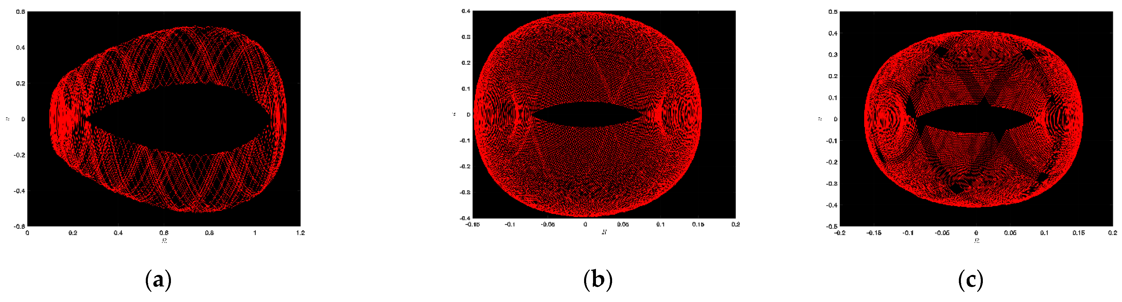
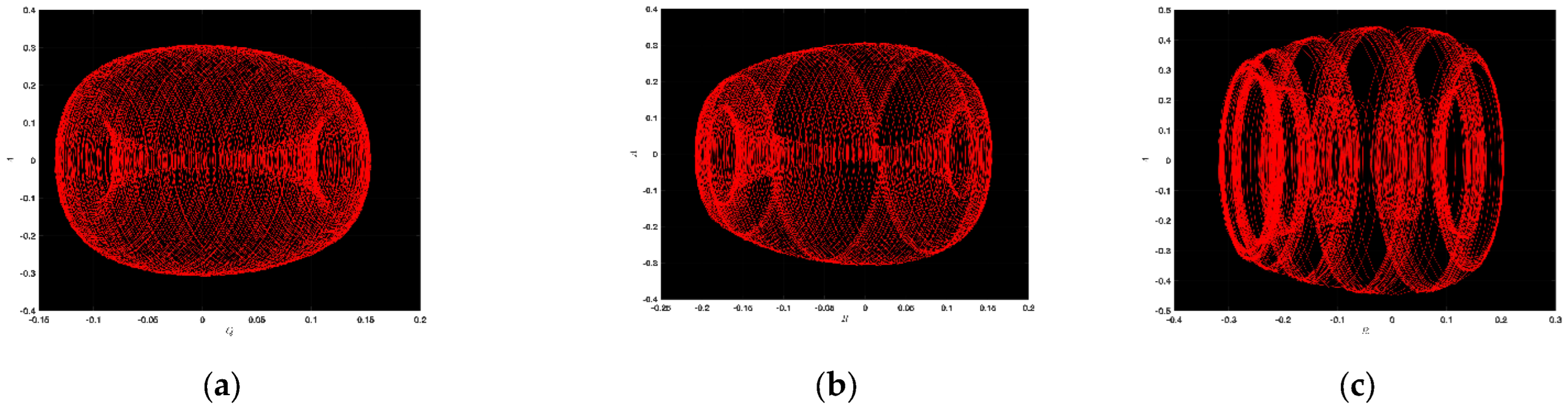
4.1. Chaotic Analysis of SNNVS

Here, we utilize the Galilean transformation for Equation (45), which supplies us with the ensuing planer dynamical system [53,54,55,56],

$$\left\{\begin{array}{c}\frac{dA\left(\tau \right)}{d\tau }=R \\ \frac{dR\left(\tau \right)}{d\tau }=W_3{A}^2\left(\tau \right)+W_{4}A\left(\tau \right) \end{array},\right.$$

(46)

wherein $W_3=M_2=\frac{3}{mn}, W_4=-M_1=-\frac{sm+qn-p}{k{m}^3+r{n}^3}$. To accomplish the chaotic nature of the declared equation, the perturbation term ${\zeta }_3\mathit{cos}\left({\zeta }_{4}t\right)$, having the magnitude ${\zeta }_3$ and the frequency ${\zeta }_4$, is added into the dynamical system declared in Equation (46):

$$\left\{\begin{array}{l}\frac{dA\left(t\right)}{dt}=R \\ \frac{dR\left(t\right)}{dt}=W_3{A}^2\left(t\right)+W_{4}A\left(t\right)+{\zeta }_3\mathit{cos}\left({\zeta }_{4}t\right) \end{array}.\right.$$

(47)

We illustrate the chaotic character of the advocated dynamical system along with the abundant values of the parameters. In Figure 6a, $s=1, q=1, p=1, r=1, k=1, m=1, n=1, {\zeta }_3=1, \mathrm{and} {\zeta }_4=\pi /2$; in Figure 6b, $s=3, q=2, p=2, r=2, k=1, m=-2, n=1, {\zeta }_3=1, \mathrm{and} {\zeta }_4=\pi /2$; in Figure 6c, $s=-3, q=2, p=2, r=2, k=1, m=-2, n=1, {\zeta }_3=1, \mathrm{and} {\zeta }_4=\pi /2$; in Figure 7a, $s=-3, q=1, p=3, r=2, k=1, m=-2, n=1, {\zeta }_3=1, \mathrm{and} {\zeta }_4=\pi$; in Figure 7b, $s=1, q=1, p=1, r=1, k=1, m=-3, n=-3, {\zeta }_3=1, \mathrm{and} {\zeta }_4=\pi$; in Figure 7c, $s=2, q=-3, p=3, r=-3, k=4, m=2, n=3, {\zeta }_3=1, \mathrm{and} {\zeta }_4=\pi$; in Figure 8a, $s=2, q=2, p=1, r=1, k=1, m=1, n=1, {\zeta }_3=1, \mathrm{and} {\zeta }_4=2\pi$; in Figure 8b, $s=2, q=2, p=1, r=1, k=2, m=-1, n=1, {\zeta }_3=1, \mathrm{and} {\zeta }_4=2\pi$; and in Figure 8c, $s=2, q=1, p=3, r=1, k=2, m=1, n=-2, {\zeta }_3=2, \mathrm{and} {\zeta }_4=2\pi$.

Now, it is evident from the demonstrated figure that complex dynamics are presented in Figure 6a, and also that the limit cycles are presented in Figure 6b,c. Moreover, strange dynamics are offered in Figure 7a,c; also, in Figure 7c, one can see the periodic dynamics. In addition, Figure 8a,b supplies us the surprising nature along with Figure 8c, which gives us the periodic dynamics. From the above observation, we are confident that this analysis detects insights into the dynamical system and that it might be valuable as well as advantageous in modern physics, advanced mathematics, and innovative engineering.

4.2. Sensitivity Analysis of SNNVS

Here, the sensitivity of the dynamical system in Equation (46) is reviewed. To finalize its sensitivity, we choose the definite value of the parameters $s=2, q=2, p=1, r=1, k=1, m=1, n=1, \mathrm{and} \beta =1$. We also set the initial conditions for the selected dynamical system as follows [53,54,55,56]:

(i)

$A\left(0\right)=0.2$ and $R=0$;

(ii)

$A\left(0\right)=0$ and $R=0.2$;

(iii)

$A\left(0\right)=0.3$ and $R=0$;

(iv)

$A\left(0\right)=0$ and $R=0.3$

In Figure 9, the sensitivity nature of the proposed system for numerous situations of initial positions are depicted, where the dynamics of class $A$ and the dynamics of class $R$ are symbolized by blue curves and orange curves, respectively. From a close inspection of Figure 9, we realize a major change in the dynamical system’s nature, where one could employ a tiny alteration in the initial position.

4.3. Bifurcation and Phase Portrait Analysis of SNNVS

The dynamical system in Equation (46) offers the Hamiltonian function [53,54,55,56],

$${\mathcal{H}}_2\left(A,R\right)=\frac{R^2}{2}-\frac{W_3{A}^3}{3}-\frac{W_4{A}^2}{2}={\mathcal{h}}_2.$$

Herein, the Hamiltonian constant is identified by ${\mathcal{h}}_2$. Now, the equilibrium standpoints $\left(0, 0\right), \left(-\frac{W_4}{W_3}, 0\right)$ can be determined after the resolution of the dynamical system in Equation (46),

$$\left\{\begin{array}{l}R=0 \\ {W_{3}A}^2+W_{4}A=0\end{array}\right..$$

Using the dynamical system in Equation (46), we obtain the Jacobian form as

$${\mathcal{D}}_2\left(A,R\right)=\left|\begin{array}{cc}0& 1\\ 2W_{3}A+W_4& 0\end{array}\right|=-2W_{3}A-W_4.$$

One might know the following decisions from Planar dynamical systems [53,54,55,56]:

• The equilibrium standpoint $\left(A,R\right)$ refer to a saddle point, while ${\mathcal{D}}_2\left(A,R\right)<0$;
• The equilibrium standpoint $\left(A,R\right)$ means a center point, while ${\mathcal{D}}_2\left(A,R\right)>0$;
• The equilibrium standpoint $\left(A,R\right)$ implies a cuspid point, while ${\mathcal{D}}_2\left(A,R\right)=0$.

Upon electing the compatible values of the parameters, we have a list of the following results:

Instance 1: $W_3>0$ and $W_4>0$

In Figure 10a, the equilibrium standpoint $\left(0, 0\right)$ shows a saddle point, and the equilibrium standpoint $\left(-0.6857, 0\right)$ shows a center point after taking the parameters as $m=3, n=2, k=-1, r=-1, s=3, p=1, \mathrm{and} q=2$.

Instance 2: $W_3<0$ and $W_4<0$

In Figure 10b, the equilibrium standpoint $\left(0, 0\right)$ displays a center point together with the equilibrium standpoint $\left(-0.5556, 0\right)$, which displays a saddle point by opting the value of the parameters as $m=1, n=-1, k=2, r=-1, s=1, p=-5, \mathrm{and} q=1$.

Instance 3: $W_3>0$ and $W_4<0$

In Figure 10c, the equilibrium standpoint $\left(0, 0\right)$ exhibits a center point, and the equilibrium standpoint $\left(1.3333, 0\right)$ exhibits a saddle point by picking the parameters as $m=1, n=1, k=2, r=-1, s=1, p=-2, \mathrm{and} q=1$.

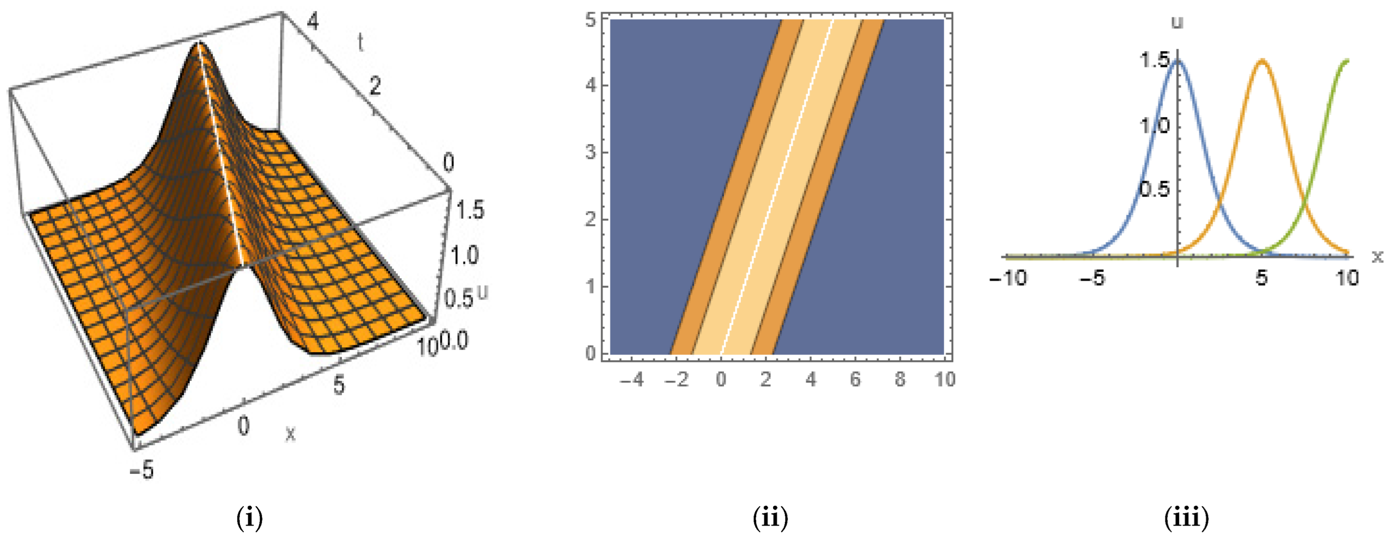
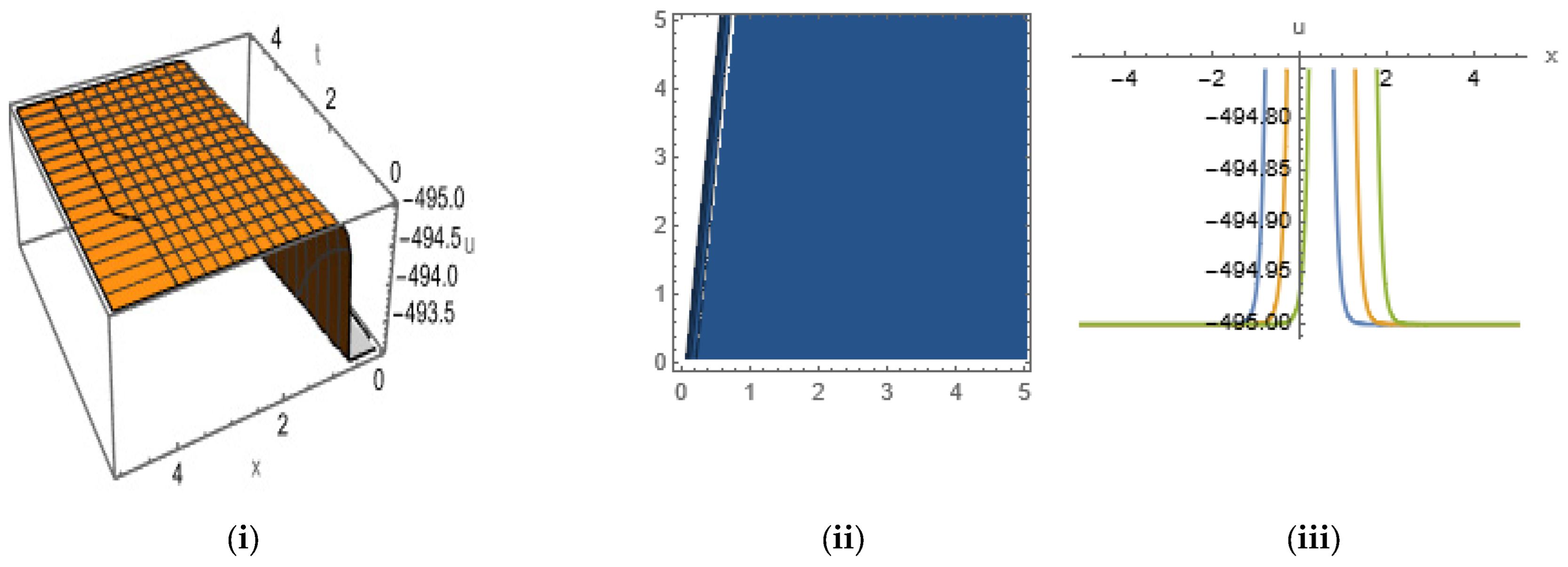
4.4. Soliton Solutions of SNNVS

Balancing the principle in Equation (45) is as follows:

$$u\left(\tau \right)=a_0+a_{1}Q\left(\tau \right)+a_2{Q}^2\left(\tau \right)+b_{1}R\left(\tau \right)+b_{2}Q\left(\tau \right)R\left(\tau \right),$$

(48)

where the functions $Q\left(\tau \right)$ and $R\left(\tau \right)$ are explained in Equations (5) and (6). Subject to the signs of λ, we obtain three cases:

Case-1. For positive values, i.e., $\lambda >0$:

By doing two times differentiation in Equation (48) and engaging Equations (6) and (8), we convert the back side of Equation (48) in $Q \mathrm{and} R$ variables. Now, balancing the coefficients in the acquired polynomial and taking zero, we gain a system of equations in the constants $a_0$,$a_1$,$a_2$, $b_1$, $b_2$, $\lambda ,$ and $c$. After finishing this action and employing the program Mathematica, we have two sets of results:

Set I:

$$a_0=\frac{-2M_1}{M_2}, a_1=0, { a}_2=\frac{3}{M_2}, b_1=\frac{-3l}{M_2}, b_2=\pm \frac{3\sqrt{\gamma M_1^2-l^2}}{\sqrt{{-M}_1}{M}_2} \mathrm{and} \lambda =-M_1; M_1<0.$$

(49)

Set II:

$$a_0=\frac{3M_1}{M_2}, a_1=0, a_2=\frac{3}{M_2}, b_1=\frac{-3l}{M_2}, b_2=\pm \frac{3\sqrt{\gamma M_1^2-l^2}}{\sqrt{M_1}{M}_2} \mathrm{and} \lambda =M_1; M_1>0.$$

(50)

For set I, we obtain the soliton solution of Equation (45),

$$u\left(\tau \right)=\frac{-2M_1}{M_2}+\frac{3\lambda }{M_2}{\left[\frac{c_1\mathit{cos}\left(\sqrt{\lambda }\tau \right)-c_2\mathit{sin}\left(\sqrt{\lambda }\tau \right)}{c_1\mathit{sin}\left(\sqrt{\lambda }\tau \right)+c_2\mathit{cos}\left(\sqrt{\lambda }\tau \right)+\frac{l}{\lambda }}\right]}^2-\frac{3l}{M_2}\frac{1}{\left[c_1\mathit{sin}\left(\sqrt{\lambda }\tau \right)+c_2\mathit{cos}\left(\sqrt{\lambda }\tau \right)+\frac{l}{\lambda }\right]}\pm \frac{3\sqrt{\lambda }\sqrt{\gamma M_1^2-l^2}}{\sqrt{{-M}_1}{M}_2}\frac{\left[c_1\mathit{cos}\left(\sqrt{\lambda }\tau \right)-c_2\mathit{sin}\left(\sqrt{\lambda }\tau \right)\right]}{{\left[c_1\mathit{sin}\left(\sqrt{\lambda }\tau \right)+c_2\mathit{cos}\left(\sqrt{\lambda }\tau \right)+\frac{l}{\lambda }\right]}^2},$$

(51)

where $\lambda =-M_1; M_1<0$. By taking $c_1=0$, and $l=0$ but $c_2\ne 0$, we attain solutions of SNNVS,

$$\begin{gathered} u\left(x,y,t\right)=\frac{-2M_1}{M_2}-\frac{3M_1}{M_2} \\ {\tan }^2\left\{\sqrt{-M_1}\left(mx+ny-pt\right)\right\}\pm \frac{{3M}_1}{M_2}\mathit{tan}\left\{\sqrt{-M_1}\left(mx+ny-pt\right)\right\}\mathit{sec}\left\{\sqrt{-M_1}\left(mx+ny-pt\right)\right\}, \end{gathered}$$

(52)

where $M_1<0$. Choosing $c_2=0$ and $l=0$ but $c_1\ne 0$,

$$u\left(x,y,t\right)=\frac{-2M_1}{M_2}-\frac{3M_1}{M_2}\left[{\mathit{cot}}^2\left\{\sqrt{-M_1}\left(mx+ny-pt\right)\right\}\pm \mathit{cot}\left\{\sqrt{-M_1}\left(mx+ny-pt\right)\right\}\mathit{cosec}\left\{\sqrt{-M_1}\left(mx+ny-pt\right)\right\}\right],$$

(53)

where $M_1<0$. For set II,

$$u\left(\tau \right)=\frac{3M_1}{M_2}+\frac{3\lambda }{M_2}{\left[\frac{c_1\mathit{cos}\left(\sqrt{\lambda }\tau \right)-c_2\mathit{sin}\left(\sqrt{\lambda }\tau \right)}{c_1\mathit{sin}\left(\sqrt{\lambda }\tau \right)+c_2\mathit{cos}\left(\sqrt{\lambda }\tau \right)+\frac{l}{\lambda }}\right]}^2-\frac{3l}{M_2}\frac{1}{\left[c_1\mathit{sin}\left(\sqrt{\lambda }\tau \right)+c_2\mathit{cos}\left(\sqrt{\lambda }\tau \right)+\frac{l}{\lambda }\right]}\pm \frac{3\sqrt{\lambda }\sqrt{\gamma M_1^2-l^2}}{\sqrt{M_1}{M}_2}\frac{\left[c_1\mathit{cos}\left(\sqrt{\lambda }\tau \right)-c_2\mathit{sin}\left(\sqrt{\lambda }\tau \right)\right]}{{\left[c_1\mathit{sin}\left(\sqrt{\lambda }\tau \right)+c_2\mathit{cos}\left(\sqrt{\lambda }\tau \right)+\frac{l}{\lambda }\right]}^2},$$

(54)

where $\lambda =M_1; M_1>0$. Similar to set I, setting $c_1=0$ and $l=0$ but $c_2\ne 0$,

$$\begin{gathered} u\left(x,y,t\right)=\frac{3M_1}{M_2} \\ {\sec }^2\left\{\sqrt{M_1}\left(mx+ny-pt\right)\right\}\pm \frac{3M_1}{M_2}\mathit{tan}\left\{\sqrt{M_1}\left(mx+ny-pt\right)\right\}\mathit{sec}\left\{\sqrt{M_1}\left(mx+ny-pt\right)\right\}, \end{gathered}$$

(55)

where $M_1>0$. For choosing $c_2=0$ and $l=0$ but $c_1\ne 0$,

$$\begin{gathered} u\left(x,y,t\right)=\frac{3M_1}{M_2} \\ {\mathit{cosec}}^2\left\{\sqrt{M_1}\left(mx+ny-pt\right)\right\}\pm \frac{3M_1}{M_2}\mathit{cot}\left\{\sqrt{M_1}\left(mx+ny-pt\right)\right\}\mathit{cosec}\left\{\sqrt{M_1}\left(mx+ny-pt\right)\right\}, \end{gathered}$$

(56)

where $M_1>0$.

Case-2. For negative values, i.e., $\lambda <0$, we find two sets:

Set I:

$$a_0=\frac{-2M_1}{M_2}, a_1=0, a_2=\frac{3}{M_2}, b_1=\frac{-3l}{M_2}, b_2=\pm \frac{3\sqrt{l^2+\delta M_1^2}}{\sqrt{M_1}{M}_2} \mathrm{and} \lambda =-M_1; M_1>0.$$

(57)

Set II:

$$a_0=\frac{3M_1}{M_2}, a_1=0, a_2=\frac{3}{M_2}, b_1=\frac{-3l}{M_2}, b_2=\pm \frac{3\sqrt{l^2+\delta M_1^2}}{\sqrt{-M_1}{M}_2} \mathrm{and} \lambda =M_1; M_1<0.$$

(58)

Similarly, for set I,

$$\begin{array}{l}u\left(\tau \right)=\frac{-2M_1}{M_2}-\frac{3\lambda }{M_2}{\left[\frac{c_1\mathit{cos}h\left(\sqrt{-\lambda }\tau \right)+c_2\mathit{sin}h\left(\sqrt{-\lambda }\tau \right)}{c_1\mathit{sin}h\left(\sqrt{-\lambda }\tau \right)+c_2\mathit{cos}h\left(\sqrt{-\lambda }\tau \right)+\frac{l}{\lambda }}\right]}^2-\frac{3l}{M_2}\frac{1}{\left[c_1\mathit{sin}h\left(\sqrt{-\lambda }\tau \right)+c_2\mathit{cos}h\left(\sqrt{-\lambda }\tau \right)+\frac{l}{\lambda }\right]}\pm \\ \frac{3\sqrt{-\lambda }\sqrt{l^2+\delta M_1^2}}{\sqrt{M_1}{M}_2}\frac{\left[c_1\mathit{cos}h\left(\sqrt{-\lambda }\tau \right)-c_2\mathit{sin}h\left(\sqrt{-\lambda }\tau \right)\right]}{{\left[c_1\mathit{sin}h\left(\sqrt{-\lambda }\tau \right)+c_2\mathit{cos}h\left(\sqrt{-\lambda }\tau \right)+\frac{l}{\lambda }\right]}^2},\end{array}$$

(59)

where $\lambda =-M_1$; $M_1>0$. Taking $c_2=0$ and $l=0$ but $c_1\ne 0$,

$$\begin{gathered} u\left(x,y,t\right)=\frac{-2M_1}{M_2}+\frac{3M_1}{M_2} \\ {\cot \mathrm{h}}^2\left\{\sqrt{M_1}\left(mx+ny-pt\right)\right\}\pm \frac{3M_1}{M_2}\mathit{cot}h\{\sqrt{M_1}\left(mx+ny-pt\right)\}\mathit{cosec}h\{\sqrt{M_1}\left(mx+ny-pt\right)\}, \end{gathered}$$

(60)

where $M_1>0$. We take set II:

$$\begin{array}{l}u\left(\tau \right)=\frac{3M_1}{M_2}-\frac{3\lambda }{M_2}{\left[\frac{c_1\mathit{cos}h\left(\sqrt{-\lambda }\tau \right)+c_2\mathit{sin}h\left(\sqrt{-\lambda }\tau \right)}{c_1\mathit{sin}h\left(\sqrt{-\lambda }\tau \right)+c_2\mathit{cos}h\left(\sqrt{-\lambda }\tau \right)+\frac{l}{\lambda }}\right]}^2-\frac{3l}{M_2}\frac{1}{\left[c_1\mathit{sin}h\left(\sqrt{-\lambda }\tau \right)+c_2\mathit{cos}h\left(\sqrt{-\lambda }\tau \right)+\frac{l}{\lambda }\right]}\pm \\ \frac{3\sqrt{-\lambda }\sqrt{l^2+\delta M_1^2}}{\sqrt{-M_1}{M}_2}\frac{\left[c_1\mathit{cos}h\left(\sqrt{-\lambda }\tau \right)-c_2\mathit{sin}h\left(\sqrt{-\lambda }\tau \right)\right]}{{\left[c_1\mathit{sin}h\left(\sqrt{-\lambda }\tau \right)+c_2\mathit{cos}h\left(\sqrt{-\lambda }\tau \right)+\frac{l}{\lambda }\right]}^2},\end{array}$$

(61)

where $\lambda =M_1$; $M_1<0$. Taking $c_2=0$ and $l=0$ but $c_1\ne 0$,

$$\begin{gathered} u\left(x,y,t\right)=\frac{3M_1}{M_2}-\frac{3M_1}{M_2}{[\cot \mathrm{h}}^2\left\{\sqrt{{-M}_1}\left(mx+ny-pt\right)\right\}\pm \mathit{cot}h\{\sqrt{{-M}_1}\left(mx+ny-pt\right)\} \\ \mathit{cosec}h\{\sqrt{{-M}_1}\left(mx+ny-pt\right)\}], \end{gathered}$$

(62)

where $M_1<0$.

Remark 1.

For$\lambda =0$, we cannot find any convenient solution using this method.

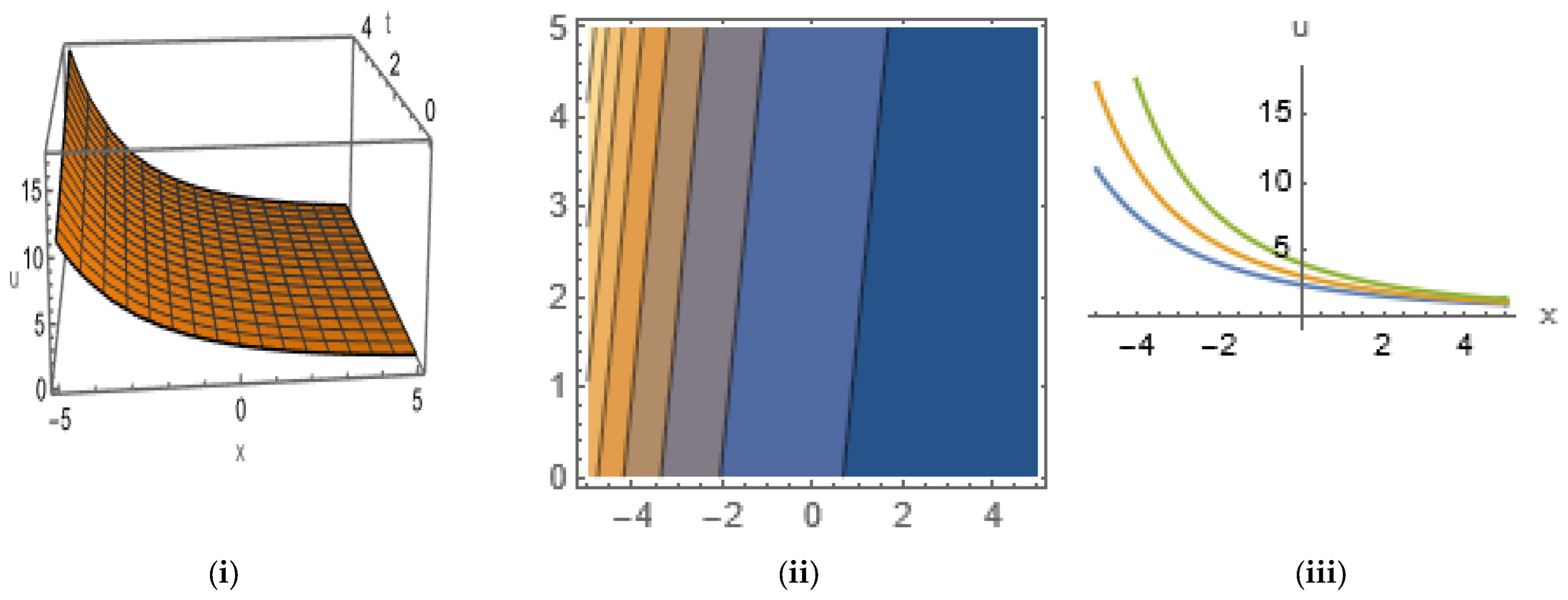
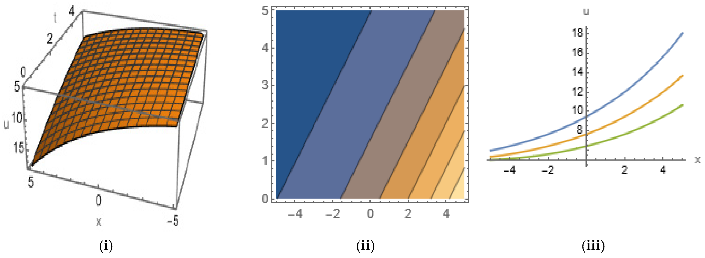
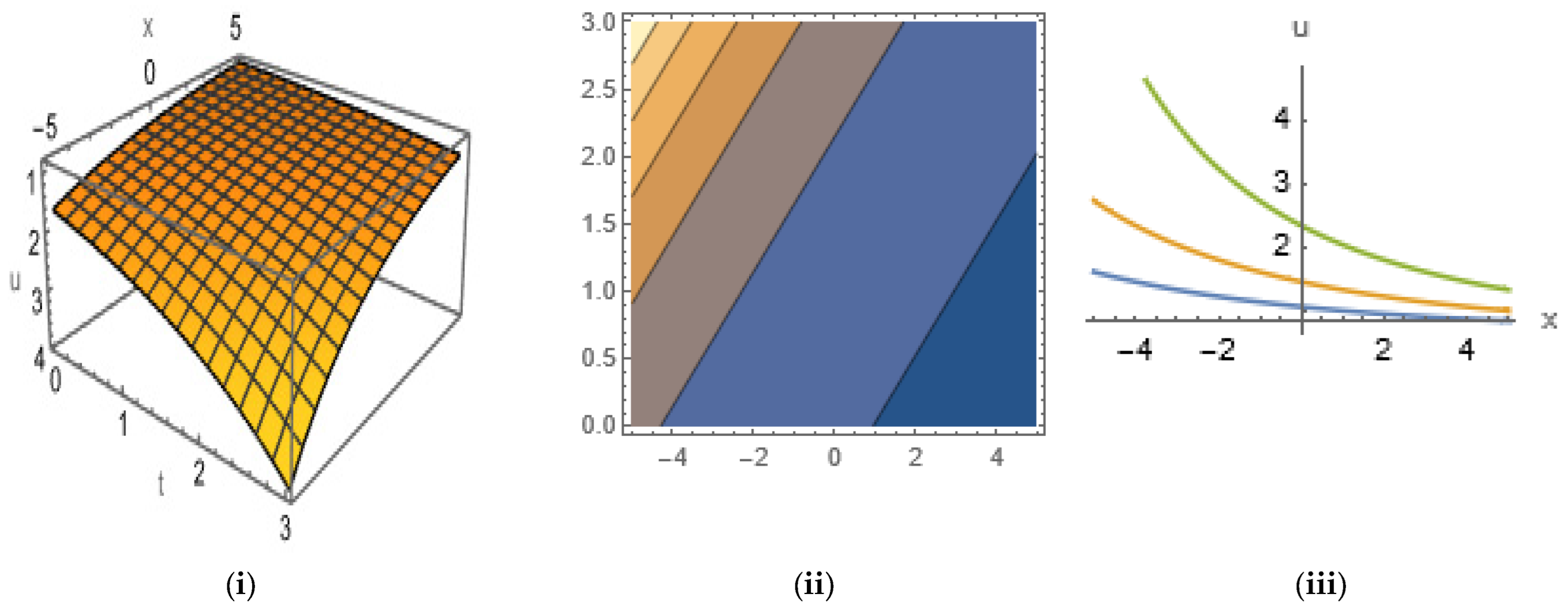
5. Graphical Representation of Soliton Solutions

In this section, we give the picturesque description of the gained solutions of the LWE and the (2 + 1)-dimensional SNNVS. The attained results are trigonometric, hyperbolic, and rational function types. The acquired results of Equations (25), (26), (28), (29), (52), (53), and (56) are of trigonometric function; the results in Equations (33), (35), (59), and (61) are of hyperbolic function; and the results in Equations (37) and (38) are of algebraic function types. For the values taken as constant, we obtain the graph of the above explicit solutions in 3D, 2D, and contour forms as given in Figure 11, Figure 12, Figure 13, Figure 14, Figure 15, Figure 16 and Figure 17.

In Figure 11, we plot Equation (25) by taking the values $\alpha =-0.01$, $\beta =2$, and $c=1$ in 3D and 2D ($t=0, 1, 5, 10$ with the range $-5\le x\le 5$) shapes, along with their contour shapes, by giving a compaction soliton within the range $x\in \left[0, 2\right]$, $t\in \left[0, 2\right]$. From the contour plot, we observe that the energy density is distributed uniformly in the region $x\in \left[1, 2\right]$, $t\in \left[0, 5\right]$, and from 2D shape we see that as time increases, figures with equal amplitudes and equal widths are displaced from left to right.

In Figure 12, we plot Equation (29) by taking the values $\alpha =2$, $\beta =1$, and $c=1$ in 3D and 2D ($t=0, 5, 10$ with the range $-5\le x\le 5$) shapes, along with their contour shapes, by giving a singular periodic solution within the range $x\in \left[-5, 5\right]$, $t\in \left[0, 5\right]$. From the contour plot, we observe that the energy density is distributed uniformly in the vertical region with $x\in \left[2.5, 3\right]$, and from 2D shape, we see that as time increases, figures with equal amplitudes and equal widths are displaced from left to right.

In Figure 13, we plot Equation (28) by taking the values $\alpha =2$, $\beta =1$, and $c=1$ in 3D and 2D ($t=0, 5, 10$ with the range $-10\le x\le 10$) shapes, along with their contour shapes, by giving a bell-shaped soliton within the range $x\in \left[-5, 10\right]$, $t\in \left[0, 5\right]$. From the contour plot, we observe that the energy density is distributed discontinuously in the inclined region $x\in \left[-2, 2\right]$, and from 2D shape, we see that as time increases, figures with equal amplitudes and equal widths are displaced from left to right.

In Figure 14, we plot Equation (35) by taking the values $\alpha =1$, $\beta =1$, and $c=0.1$ in 3D and 2D ($t=0, 5, 10$ with the range $-5\le x\le 5$) shapes, along with their contour shapes, by giving an anti-kink-shaped soliton within the range $x\in \left[0, 5\right]$, $t\in \left[0, 5\right]$. From the contour plot, we observe that the energy density is distributed uniformly except the vertical strip of the region $x\in \left[0, 0.1\right]$, $t\in \left[0, 5\right]$, and from 2D shape, we see that the amplitude remains the same, but width of the figures increases as time increases.

In Figure 15, we plot Equation (52) by taking the values $M_1=-3$, $M_2=2$, $m=0.1$, $n=0.1$, $p=0.02$, $\mathrm{and} y=1$ in 3D and 2D ($t=0, 5, 10$ with the range $-5\le x\le 5$) shapes, along with their contour shapes, by giving a one-sided, anti-kink-shaped soliton within the range $x\in \left[-5, 5\right]$, $t\in \left[0, 5\right]$. From the contour plot, we observe that the energy density is at maximum in the region $x\in \left[-4,-2\right]$, $t\in \left[0, 5\right]$, and from 2D shape, we see that the amplitude and width of the figures decrease as time increases.

In Figure 16, we plot Equation (54) by taking the values $M_1=-1$, $M_2=0.1$, $m=0.1$, $n=1$, $p=0.1$, $\mathrm{and} y=1$ in 3D and 2D ($t=0, 2, 4$ with the range $-5\le x\le 5$) shapes, along with their contour shapes, by giving a flat kink-shaped soliton within the range $x\in \left[-5, 5\right]$, $t\in \left[0, 5\right]$. From the contour plot, we observe that the energy density is at maximum in the region $x\in \left[0, 4\right]$, $t\in \left[0, 4\right]$, and from 2D shape, we see that the amplitude and width of the figures decrease as time increases.

In Figure 17, we plot Equation (56) by taking the values $M_1=1$, $M_2=2$, $m=0.1$, $n=2$, $p=0.2$, $\mathrm{and} y=1$ in 3D and 2D ($t=0, 2, 4$ with the range $-5\le x\le 5$) shapes, along with their contour shapes, by giving a compaction soliton within the range $x\in \left[-5, 5\right]$, $t\in \left[0, 3\right]$. From the contour plot, we observe that the energy density is at maximum in the region $x\in \left[-4,-2\right]$, $t\in \left[1, 3\right]$, and from 2D shape, we see that the amplitude and width of the figures decrease as time increases.

6. Conclusions

In the recent study, we successfully investigated some important analyses, chaotic phenomena, sensitivity, and bifurcation to the LWE and the SNNVS. In chaotic phenomena, we plotted different physically applicable patterns such as limit cycle, complex dynamics, ringlet dynamics, strange dynamics, periodic dynamics, etc. For both mathematical models, we applied sensitivity analyses, and we discovered that these systems’ outcomes are very sensitive to their initial states. Bifurcation analysis was exploited to figure out the equilibrium points of the relevant systems. Also, we extracted new, abundant wave soliton solutions of the mentioned equations by applying the double-variable expansion method. The graphical demonstration of the soliton solutions implies that the formations of the attained solutions are of compaction soliton, parabolic-shaped soliton, singular periodic solution, bell-shaped soliton, anti-kink-shaped soliton, one-sided kink-shaped soliton, flat kink-shaped solitons, etc. Our obtained results may be used to explore the naturalistic phenomena subject to the nonlinear partial differential equation. Finally, we have checked our results by back substitute through Mathematica software. The obtained solutions might be important for exposing the naturalistic occurrence arising in science and engineering, which can amplify the impact on posterior research work. This article will have great impact on nonlinear science due to the new solitary wave structures with different complex phenomena, sensitivity analysis, and bifurcation analysis.

References

1. Malwe, B.H.; Betchewe, G.; Doka, S.Y.; Kofane, T.C. Travelling wave solutions and soliton solutions for the nonlinear transmission line using the generalized Riccati equation mapping method. Nonlinear Dyn. 2016, 84, 171–177. [Google Scholar] [CrossRef]
2. Pandir, Y.; Gurefe, Y. A new version of the generalized F-expansion method for the fractional Biswas-Arshed equation and Boussinesq equation with the beta-derivative. J. Funct. Spaces 2023, 3, 1–14. [Google Scholar] [CrossRef]
3. Zhao, Y.M. F-expansion method and its application for finding new exact solutions to the Kudryashov-Sinelshchikov equation. J. Appl. Math. 2023, 2023, 895760. [Google Scholar] [CrossRef]
4. Na, S. Auxiliary equation method and new solutions of Klein-Gordon equation. Chaos Solitons Fractals 2007, 31, 943–950. [Google Scholar]
5. Liu, Y.; Wu, G. Using a new auxiliary equation to construct abundant solutions for nonlinear evolution equations. J. Appl. Math. Phys. 2021, 9, 12. [Google Scholar] [CrossRef]
6. SLiu, K.; Fu, Z.T.; Liu, S.D.; Zhao, Q. Jacobi elliptic function method and periodic wave solutions of nonlinear wave equations. Phys. Lett. A 2001, 289, 69–74. [Google Scholar]
7. Hussain, A.; Chahlaoui, Y.; Zaman, F.D.; Parveen, T.; Hassan, A.M. The Jacobi elliptic function method and its application for the stochastic NNV system. Alex. Eng. J. 2023, 81, 347–359. [Google Scholar] [CrossRef]
8. Seadawy, A.R.; Rashidy, K.E. Travelling wave solution for some coupled nonlinear evolution equations. Math. Comput. Model. 2013, 57, 1371–1379. [Google Scholar] [CrossRef]
9. Taghizadeh, N.; Neirameh, A.; Shokooh, S. New application of the direct algebraic method to Eckhaus equation. Trends Appl. Sci. Res. 2012, 7, 476–482. [Google Scholar] [CrossRef]
10. Ohwada, T. Cole-Hopf transformation as a numerical tool for the Burgers equation. Appl. Comput. Math. 2009, 8, 107–113. [Google Scholar]
11. Rong, F.; Li, Q.; Shi, B.; Chai, Z. A lattice Boltzmann model based on Cole-Hopf transformation for N-dimensional coupled Burgers’ equations. Comput. Math. Appl. 2023, 134, 101–111. [Google Scholar] [CrossRef]
12. Mamun, A.A.; Ananna, S.N.; Gharami, P.P.; An, T.; Asaduzzaman, M. The improved modified extended tanh-function method to develop the exact travelling wave solutions of a family of 3D fractional WBBM equations. Results Phys. 2022, 41, 105969. [Google Scholar] [CrossRef]
13. Wang, X.; Wu, J.; Wu, J.; Wang, Y.; Chen, C. Extended tanh-function method and its applications in nonlocal complex mKdV equations. Mathematics 2022, 10, 3250. [Google Scholar] [CrossRef]
14. Carillo, S.; Schiebold, C. Soliton equations: Admitted solutions and invariances via Bäcklund transformations. Open Commun. Nonlinear Math. Phys. 2024, 1, 1–11. [Google Scholar] [CrossRef]
15. Liu, J.G.; He, Y. New periodic solitary wave solutions for the (3+1)-dimensional generalized shallow water equation. Nonlinear Dyn. 2017, 90, 363–369. [Google Scholar] [CrossRef]
16. Wazwaz, A.M. The Hirota’s bilinear method and the tanh-coth method for multiple-soliton solutions of the Sawada-Kotera-Kadomstsev-Petviashvili equation. Appl. Math. Comput. 2008, 200, 160–166. [Google Scholar]
17. Kumar, S.; Mohan, B. A novel and efficient method for obtaining Hirota’s bilinear form for the nonlinear evolution equation in (n+1)-dimensions. Partial. Differ. Equ. Appl. Math. 2022, 5, 100274. [Google Scholar] [CrossRef]
18. Ghanbari, B. Employing Hirota’s bilinear form to find novel lump waves solutions to an important nonlinear model in fluid mechanics. Results Phys. 2021, 29, 104689. [Google Scholar] [CrossRef]
19. Chadwick, E.; Hatam, A.; Kazem, S. Exponential function method for solving nonlinear ordinary differential equations with constant coefficients on a semi-infinite domain. Proc.-Indian Acad. Math. Sci. 2016, 126, 79–97. [Google Scholar] [CrossRef]
20. Kadkhoda, N.; Jafari, H. Analytical solutions of the Gerdjikov-Ivanov equation by using exp(−Φ(ξ))-expansion method. Optic 2017, 139, 72–76. [Google Scholar] [CrossRef]
21. Rahman, M.M.; Habib, M.A.; Ali, H.M.S.; Miah, M.M. The generalized Kudryashov method: A renewed mechanism for performing exact solitary wave solutions of some NLEEs. J. Mech. Contin. Math. Sci. 2019, 14, 323–339. [Google Scholar] [CrossRef]
22. Ekici, M. Exact solutions to some nonlinear time-fractional evolution equations using the generalized Kudryashov method in mathematical physics. Symmetry 2023, 15, 1961. [Google Scholar] [CrossRef]
23. Yousif, A.A.; AbdulKhaleq, F.A.; Mohsin, A.K.; Mohammed, O.H.; Malik, A.M. A developed technique of homotopy analysis method for solving nonlinear systems of Volterra integro-differential equations of fractional order. Partial. Differ. Equ. Appl. Math. 2023, 8, 100548. [Google Scholar] [CrossRef]
24. Gusu, D.M.; Gudeta, W. Solving Nonlinear Partial Differential Equations of Special Kinds of 3rd Order Using Balance Method and Its Models. Int. J. Differ. Equ. 2023, 2023, 7663326. [Google Scholar] [CrossRef]
25. Wang, M.; Li, X. Simplified homogeneous balance method and its applications to the Whitham-Broer-Kaup model equations. J. Appl. Math. Phys. 2014, 2, 8. [Google Scholar] [CrossRef]
26. Zayed, E.M.E.; Alurrfi, K.A.E. The homogeneous balance method and its applications for finding the exact solutions for nonlinear evolution equations. Ital. J. Pure Appl. Math. 2014, 33, 307–318. [Google Scholar]
27. Neamaty, A.; Agheli, B.; Darzi, R. Variational iteration method and He’s polynomials for time-fractional partial differential equations. Prog. Fract. Differ. Appl. 2015, 1, 47–55. [Google Scholar]
28. Pham, V.H.S.; Dang, N.T.N.; Nguyen, V.N. Enhancing engineering optimization using hybrid sine cosine algorithm with Roulette wheel selection and opposition-based learning. Sci. Rep. 2024, 14, 694. [Google Scholar] [CrossRef] [PubMed]
29. Iqbal, M.A.; Miah, M.M.; Ali, H.M.S.; Shahen, N.H.M.; Deifalla, A. New applications of the fractional derivative to extract abundant soliton solutions of the fractional order PDEs in mathematics physics. Partial. Differ. Equ. Appl. Math. 2024, 9, 100597. [Google Scholar] [CrossRef]
30. Iqbal, M.A.; Miah, M.M.; Rasid, M.M.; Alshehri, H.M.; Osman, M.S. An investigation of two integro-differential KP hierarchy equations to find out closed form solitons in mathematical physics. Arab. J. Basic Appl. Sci. 2023, 30, 535–545. [Google Scholar] [CrossRef]
31. Ganie, A.H.; Sadek, L.H.; Tharwat, M.M.; Iqbal, M.A.; Miah, M.M.; Rasid, M.M.; Elazab, N.S.; Osman, M.S. New investigation of the analytical behaviors for some nonlinear PDEs in mathematical physics and modern engineering. Partial. Differ. Equ. Appl. Math. 2024, 9, 100608. [Google Scholar] [CrossRef]
32. Wang, M.; Li, X.; Zhang, J. The (G’/G)-expansion method and travelling wave solutions of nonlinear evolution equation in mathematical physics. Phys. Lett. A 2008, 372, 417–423. [Google Scholar]
33. Khan, A.T.; Naher, H. Some New Non-Travelling Wave Solutions of the Fisher Equation with Nonlinear Auxiliary Equation. Orient. J. Phys. Sci. 2018, 3, 92–101. [Google Scholar] [CrossRef]
34. Naher, H.; Abdullah, F.A. New approach of (G’/G)-expansion method and new approach of generalized (G’/G)-expansionmethod for nonlinear evolution equation. AIP Adv. 2013, 3, 032116. [Google Scholar] [CrossRef]
35. Zayed, E.M.E. The (G’/G)-expansion method and its applications to some nonlinear evolution equations in the mathematical physics. J. Appl. Math. Comput. 2009, 30, 89–103. [Google Scholar] [CrossRef]
36. Shakeel, M.; Mohyud-Din, S.T. Modified (G’/G)-expansion method with generalized Riccati equation to the sixth-order Boussinesq equation. Ital. J. Pure Appl. Math. 2013, 30, 393–410. [Google Scholar]
37. Saba, F.; Jabeen, S.; Akbar, H.; Mohyud-Din, S.T. Modified alternative (G’/G)-expansion method to general Sawada-Kotera equation of fifth-order. J. Egypt. Math. Soc. 2015, 23, 416–423. [Google Scholar] [CrossRef]
38. Zhu, M. Solving the Burgers-Huxley equation by (G’/G)-expansion method. J. Appl. Math. Phys. 2016, 4, 7. [Google Scholar] [CrossRef]
39. Bin, Z. (G’/G)-expansion method for solving fractional partial differential equations in the theory of mathematical physics. Commun. Theor. Phys. 2012, 58, 623. [Google Scholar]
40. Akçağıl, Ş.; Aydemir, T. Comparison between the (G’/G)-expansion method and the modified extended tanh method. Open Phys. 2016, 14, 88–94. [Google Scholar] [CrossRef]
41. Iqbal, M.A.; Baleanu, D.; Miah, M.M.; Ali, H.M.S.; Alshehri, H.M.; Osman, M.S. New soliton solutions of the mZK equation and the Gerdjikov-Ivanov equation by employing the double (G’/G, 1/G)-expansion method. Results Phys. 2023, 47, 106391. [Google Scholar] [CrossRef]
42. Miah, M.M.; Seadawy, A.R.; Ali, H.M.S.; Akbar, M.A. Abundant closed form wave solutions to some nonlinear evolution equations in mathematical physic. J. Ocean. Eng. Sci. 2020, 5, 269–278. [Google Scholar] [CrossRef]
43. Iqbal, M.A.; Wang, Y.; Miah, M.M.; Osman, M.S. Study on Date-Jimbo-Kashiwara-Miwa equation with conformable derivative dependent on time parameter to find the exact dynamic wave solutions. Fractal Fract. 2022, 6, 4. [Google Scholar] [CrossRef]
44. Inc, M.; Miah, M.M.; Chowdhury, A.; Ali, H.M.S.; Rezazadeh, H.; Akinlar, M.A.; Chu, Y.M. New exact solutions for Kaup-Kupershmidt equation. AIMS Math. 2020, 5, 6726–6738. [Google Scholar] [CrossRef]
45. Sirisubtawee, S.; Koonprasert, S.; Sungnul, S. Some applications of the (G’/G, 1/G)expansion method for finding exact traveling wave solutions of nonlinear fractional evolution equations. Symmetry 2019, 11, 952. [Google Scholar] [CrossRef]
46. Hossain, M.N.; Alsharif, F.; Miah, M.M.; Kanan, M. Abundant New Optical Soliton Solutions to the Biswas–Milovic Equation with Sensitivity Analysis for Optimization. Mathematics 2024, 12, 1585. [Google Scholar] [CrossRef]
47. Chowdhury, M.A.; Miah, M.M.; Iqbal, M.A.; Alshehri, H.M.; Baleanu, D.; Osman, M.S. Advanced exact solutions to the nano-ionic currents equation through MTs and the soliton equation containing the RLC transmission line. Eur. Phys. J. Plus 2023, 138, 502. [Google Scholar] [CrossRef]
48. Miah, M.M.; Iqbal, M.A.; Osman, M.S. A study on stochastic longitudinal wave equation in a magneto-electro-elastic annular bar to find the analytical solutions. Commun. Theor. Phys. 2023, 75, 085008. [Google Scholar] [CrossRef]
49. Duran, S. Travelling wave solutions and simulation of the Lonngren wave equation for tunnel diode. Opt. Quantum Electron. 2021, 53, 8. [Google Scholar] [CrossRef]
50. Roshid, M.M.; Rahman, M.M.; Bashar, M.H.; Hossain, M.M.; Mannaf, M.A.; Roshid, H.O. Dynamical simulation of wave solutions for the M-fractional Lonngren wave equation using two distinct methods. Alex. Eng. J. 2023, 81, 460–468. [Google Scholar] [CrossRef]
51. Ahmad, J.; Mustafa, Z.; Rehman, S.U.; Turki, N.B.; Shah, N.A. Solitary wave structures for the stochastic Nizhnik-Novikov-Veselov system via modified generalized rational exponential function method. Results Phys. 2023, 52, 106776. [Google Scholar] [CrossRef]
52. Shaikh, T.S.; Baber, M.Z.; Ahmed, N.; Iqbal, M.S.; Akgül, A.; Din, S.M.E. Investigation of solitary wave structures for the stochastic Nizhnik–Novikov–Veselov (SNNV) system. Results Phys. 2023, 48, 106389. [Google Scholar] [CrossRef]
53. Jhangeer, A.; Almusawa, H.; Hussain, Z. Bifurcation study and pattern formation analysis of a nonlinear dynamical system for chaotic behavior in traveling wave solution. Results Phys. 2022, 37, 105492. [Google Scholar] [CrossRef]
54. Li, Z.; Hu, H. Chaotic pattern, bifurcation, sensitivity and traveling wave solution of the coupled Kundu-Mukherjee-Naskar equation. Results Phys. 2023, 48, 106441. [Google Scholar] [CrossRef]
55. Rafiq, M.H.; Raza, N.; Jhangeer, A. Dynamic study of bifurcation, chaotic behavior and multi-soliton profiles for the system of shallow water wave equations with their stability. Chaos Solitons Fractals 2023, 171, 113436. [Google Scholar] [CrossRef]
56. Wang, P.; Yin, F.; Rahman, M.U.; Khan, M.A.; Baleanu, D. Unveiling complexity: Exploring chaos and solitons in modified nonlinear Schrödinger equation. Results Phys. 2024, 56, 107268. [Google Scholar] [CrossRef]
Figure 1. Chaotic patterns of the offered dynamical system with specific values of the parameters together with ζ 2 = π / 2 .
Mathematics 12 01959 g001
Figure 2. Chaotic patterns of the offered dynamical system with several values of the parameters together with ζ 2 = π .
Mathematics 12 01959 g002
Figure 3. Chaotic patterns of the offered dynamical system with numerous definite values of the parameters together with ζ 2 = 2 π .
Mathematics 12 01959 g003
Figure 4. Sketch of the sensitivity analysis of the proposed dynamical system upon considering several values of the parameters alongside some initial conditions: (a) u 0 = 0.1 and R = 0 , (b) u 0 = 0 and R = 0.1 , (c) u 0 = 0.15 and R = 0 and (d) u 0 = 0 and R = 0.15 .
Mathematics 12 01959 g004
Figure 5. Bifurcation and phase portrait analyses of the proposed system using different values of the parameters together with miscellaneous states for W 1 and W 2 .
Mathematics 12 01959 g005
Figure 6. Chaotic patterns of the mentioned dynamical system along with many values of the parameters, including ζ 4 = π / 2 .
Mathematics 12 01959 g006
Figure 7. Chaotic patterns of the mentioned dynamical system together with diverse values of the parameters, including ζ 4 = π .
Mathematics 12 01959 g007
Figure 8. Chaotic patterns of the mentioned dynamical system with several values of the parameters, including ζ 4 = 2 π .
Mathematics 12 01959 g008
Figure 9. Sketch of the sensitivity analysis of the proposed dynamical system made by choosing different values of the parameters with specific initial conditions: (a) A 0 = 0.2 and R = 0 , (b) A 0 = 0 and R = 0.2 , (c) A 0 = 0.3 and R = 0 , and (d) A 0 = 0 and R = 0.3 .
Mathematics 12 01959 g009
Figure 10. Bifurcation and phase portrait analyses of the proposed system using different values of the parameters together with miscellaneous states for W 3 and W 4 .
Mathematics 12 01959 g010
Figure 11. The (i) 3D, (ii) contour, and (iii) 2D shapes that have compaction solitons for Equation (25) with the given set of parameters.
Mathematics 12 01959 g011
Figure 12. The (i) 3D, (ii) contour, and (iii) 2D shapes that have singular periodic solitons for Equation (29) with the given set of parameters.
Mathematics 12 01959 g012
Figure 13. The (i) 3D, (ii) contour, and (iii) 2D shapes that have bell-shaped solitons for Equation (33) with the given set of parameters.
Mathematics 12 01959 g013
Figure 14. The (i) 3D, (ii) contour, and (iii) 2D shapes that have anti-kink-shaped solitons for Equation (35) with the given set of parameters.
Mathematics 12 01959 g014
Figure 15. The (i) 3D, (ii) contour, and (iii) 2D shapes that have one-sided anti-kink-shaped solitons for Equation (52) with the given set of parameters.
Mathematics 12 01959 g015
Figure 16. The (i) 3D, (ii) contour, and (iii) 2D shapes that have flat kink-shaped solitons for Equation (53) with the given set of parameters.
Mathematics 12 01959 g016
Figure 17. The (i) 3D, (ii) contour, and (iii) 2D shapes that have compaction solitons for Equation (56) with the given set of parameters.
Mathematics 12 01959 g017
Disclaimer/Publisher’s Note: The statements, opinions and data contained in all publications are solely those of the individual author(s) and contributor(s) and not of MDPI and/or the editor(s). MDPI and/or the editor(s) disclaim responsibility for any injury to people or property resulting from any ideas, methods, instructions or products referred to in the content.