Multi-View and Multimodal Graph Convolutional Neural Network for Autism Spectrum Disorder Diagnosis

Abstract

Autism Spectrum Disorder (ASD) presents significant diagnostic challenges due to its complex, heterogeneous nature. This study explores a novel approach to enhance the accuracy and reliability of ASD diagnosis by integrating resting-state functional magnetic resonance imaging with demographic data (age, gender, and IQ). This study is based on improving the spectral graph convolutional neural network (GCN). It introduces a multi-view attention fusion module to extract useful information from different views. The graph’s edges are informed by demographic data, wherein an edge-building network computes weights grounded in demographic information, thereby bolstering inter-subject correlation. To tackle the challenges of oversmoothing and neighborhood explosion inherent in deep GCNs, this study introduces DropEdge regularization and residual connections, thus augmenting feature diversity and model generalization. The proposed method is trained and evaluated on the ABIDE-I and ABIDE-II datasets. The experimental results underscore the potential of integrating multi-view and multimodal data to advance the diagnostic capabilities of GCNs for ASD.

1. Introduction

Autism Spectrum Disorder (ASD) is a complex developmental condition characterized by challenges in social interaction, communication, and repetitive behaviors [1]. According to the World Health Organization, approximately 1 in 100 children worldwide have ASD. Although the exact causes of ASD remain elusive, a combination of genetic and environmental factors is thought to contribute to its development. Symptoms usually emerge in early childhood, emphasizing the importance of early intervention for better outcomes. Treatment strategies, including behavioral, speech, and occupational therapies, are tailored to individual needs, focusing on enhancing communication, social skills, and daily functioning [2]. While there is no cure for ASD, these interventions can significantly improve the quality of life. Increased prevalence has not only spurred more research into understanding and treating ASD but also fostered more supportive communities for individuals and families affected by the condition.

Earlier machine learning models like Support Vector Machine (SVM), Random Forest (RF), Neural Networks, etc., were able to identify ASD and healthy individuals. Even though the early accuracy was not high, this still brings new hope for the application of AI to the automated diagnosis of ASD. With the development of artificial intelligence (AI), the emergence of deep learning, especially increasingly rich convolutional neural networks, has improved the accuracy of automatic ASD diagnosis. In addition to AI, medical technology is also advancing, with more and more data from different modalities being used for doctors’ diagnoses. Additionally, this data help to improve the performance of deep learning models.

Currently, there are still many issues with using artificial intelligence technology to achieve the automatic diagnosis of ASD. Firstly, researchers have different segmentation methods for brain rs-fMRI, where different brain regions have different functions. These variations in segmentation lead to information loss, making the accurate diagnosis of ASD difficult. Secondly, with the development of medical technology, data from different modalities are increasingly abundant, making the effective utilization of multimodal data an important issue. Lastly, models adapted for multi-view and multimodal data often suffer from insufficient feature representation and unreasonable model structures, making it difficult to effectively integrate data. To address these issues, this paper proposes an improved spectral graph convolutional neural network method for the automatic diagnosis of ASD, called MMGCN. The main contributions of this paper are as follows:

• Multi-View Attention Fusion Module: We introduce a novel module that integrates multiple views of fMRI data, enhancing the network’s ability to capture comprehensive features that are crucial for accurate ASD diagnosis.
• Edge-Building Network Informed by Demographic Data: By incorporating demographic factors such as age and gender, we construct a more informed graph structure, enhancing inter-subject connectivity and relevance.
• Advanced Graph Structure Techniques: We have combined DropEdge regularization with residual connections to combat the common issues of oversmoothing and neighborhood explosion in deep graph convolutional networks. DropEdge selectively drops edges during training to enhance model robustness and prevent overfitting, while residual connections preserve feature diversity and improve generalization across various data presentations.
• Validation and Evaluation on Public Datasets: The enhanced model was rigorously trained and evaluated using the ABIDE-I and ABIDE-II datasets. Our experimental results demonstrate the superiority of our approach compared to existing methods, showcasing its effectiveness in leveraging complex multimodal data for medical diagnostics.

The structure of this paper is as follows: Section 2 provides a literature review and summary of the related work involved in this study. Section 3 introduces the dataset and data preprocessing, providing a detailed explanation of the proposed method. Section 4 presents the results and analysis of parameter analysis, ablation experiments, and comparative experiments conducted on two publicly available datasets. Section 5 summarizes the entire paper and discusses the limitations of the proposed method and future work.

2. Related Work

As medical artificial intelligence progresses, leveraging machine learning technologies for the analysis of medical data, especially imaging data, facilitates the automation of ASD diagnosis.

Wang et al. [3] introduce a novel approach utilizing SVM-RFE on rs-fMRI data to classify autism and control groups with improved accuracy, achieving 90.60% classification accuracy globally and 75.00–95.23% across different sites, highlighting the potential of this FC-based algorithm for enhancing autism diagnosis by accurately identifying the most discriminative brain connectivity features from large datasets. Xu et al. [4] employ an XGB machine learning model to diagnose autism severity in children by analyzing the relationship between their physical fitness and gray matter volume, achieving high accuracy and offering insights into the factors influencing autism severity. Rathore et al. [5] examine topological features for autism classification with fMRI data, using neural networks, SVMs, and RF. They introduce a hybrid model combining topological and correlation features but note that improvements are not consistently significant, cautioning on their reliability in neuroimaging for autism diagnosis. Chen et al. [6] introduce a multimodal framework for early ASD identification in children, integrating eye fixation, facial expression, and cognitive data. Their study employs an optimized RF algorithm and hybrid data fusion, achieving 91% accuracy. Wang et al. [7] propose a multi-center low-rank representation learning method for autism spectrum disorder diagnosis, utilizing rs-fMRI data. Their study transforms data from various centers into a common latent space for classification using the k-nearest neighbor algorithm, demonstrating improved accuracy over other methods. Mostafa et al. [8] employ feature selection to identify 64 discriminative features and achieve 77.7% classification accuracy with Linear Discriminant Analysis, outperforming existing methods.

In recent years, advances in deep learning, especially in convolutional neural networks, have facilitated the development of automatic ASD diagnosis. Guo et al. [9] distinguished ASD from typically developing controls using conventional MRI and ADC data. The primary model, based on ResNet-18, was trained on multiple MRI sequences and evaluated with high performance in FLAIR and ADC sequences, potentially offering new radiological insights into ASD diagnosis. Epalle et al. [10] developed a DNN for ASD classification using ABIDE I data, incorporating multiple atlases for feature learning. The model, trained with hinge loss, achieved higher accuracy than prior methods, highlighting the value of multi-atlas data fusion for improving ASD detection. Ma et al. [11] utilized deep learning with GANs on ABIDE fMRI data to explore amygdala FC in ASD. They identified the slow-5 frequency band as the most accurate for classifying ASD, revealing frequency-specific neural markers and advancing our understanding of ASD’s pathology. Heinsfeld et al. [12] applied deep learning algorithms to the ABIDE dataset to identify neural patterns associated with ASD. Their method combined supervised and unsupervised machine learning, achieving 70% accuracy in classifying ASD versus control subjects. The study revealed an anticorrelation in brain function between anterior and posterior areas in ASD, supporting the anterior–posterior disruption theory in brain connectivity for this disorder. The findings enhance the understanding of ASD’s neural underpinnings and demonstrate the potential of deep learning for analyzing large, heterogeneous brain imaging datasets.

Over the last three years, an increasing number of studies have focused on the automated diagnosis of ASD. Lu et al. [13] developed DeepTSK, a deep learning model that combines MO-TSK FIS for feature extraction and a deep belief network for ASD classification, achieving improved accuracy and interpretability in identifying discriminative functional connectivities from ABIDE datasets. Kashef [14] proposed an enhanced convolutional neural network (ECNN) for diagnosing ASD using brain imaging data from the ABIDE database. The ECNN model utilizes temporal convolutional layers with causal convolutions and dilations, effectively capturing functional connectivity patterns for ASD identification. Experimental results showed that the ECNN achieved 80% accuracy, revealing an inverse correlation between front and back brain functions. Ahmed et al. [15] designed a single volume image generator to convert 4D fMRI data into 2D three-channel images, capturing voxel time points individually. They then utilized these images to train an improved CNN for classifying autism spectrum disorder and typical controls. The study implemented a deep ensemble learning framework, combining CNN with VGG16 features for enhanced classification accuracy. Zhang et al. [16] proposed a deep learning approach with F-score feature selection for diagnosing ASD using fMRI functional connectivity data, achieving high accuracy and offering insights into brain network topology in ASD. The method achieved an average accuracy of 64.53% on intra-site datasets and 70.9% on the ABIDE dataset, revealing a shift from small-world to random network architecture in autism spectrum disorder.

The review of existing automated diagnostic methods for ASD underscores the significant impact of machine learning and deep learning technologies on medical imaging analysis. Techniques such as SVM, RF, neural networks, and CNN have notably improved the accuracy and efficiency of diagnosing ASD. These methods excel at differentiating ASD from control groups through functional connectivity-based algorithms and enhance diagnostic accuracy by integrating multimodal data, including eye movement, facial expressions, and cognitive assessments. Advanced deep learning approaches, employing models like ResNet-18 and GANs, further advance ASD diagnosis by applying sophisticated feature extraction and classification techniques to MRI and fMRI data. Despite these advancements, challenges remain with data variability, model generalization across diverse populations, and the integration of multimodal information. These challenges frame key areas for ongoing research, aiming to refine diagnostic tools to enhance their application and reliability universally. This analysis not only highlights the progress made in the automated diagnosis of ASD but also pinpoints the persistent obstacles that future efforts need to address.

3. Materials and Methods

This study utilizes two modalities of data, namely fMRI and demographic information, to construct the nodes and edges of the graph, respectively. Preprocessed fMRI data from different views undergo feature extraction through two denoising autoencoders to obtain low-dimensional features, followed by feature dimension standardization. Subsequently, the data from different views are aggregated together through global average pooling (GAP) [17]. Weight vectors for different views are learned via a Multilayer Perceptron (MLP) [18], and new feature representations are obtained from the feature function. These obtained features are used to construct the nodes of the graph. The edges of the graph are formed by cosine similarity between pairs of subjects based on demographic information such as age, gender, and IQ, calculated through an edge-building network. The constructed input graph passes through a GCN model consisting of modules such as CL, CLD, and DCL to obtain the output graph, where C represents convolutional layers, L represents the Leaky ReLU activation function, and D represents DropEdge. Additionally, the GCN applies DropEdge and residual connections to alleviate oversmoothing and the problem of neighborhood explosion. The proposed MMGCN is shown in Figure 1.

3.1. Datasets and Data Preprocessing

This study conducts research on diagnosing autism spectrum disorder using two publicly available datasets, ABIDE-I [19] and ABIDE-II [20]. The ABIDE datasets are made accessible to researchers with the aim of promoting data sharing and collaborative research to advance the understanding of autism. All research in this manuscript complies with all relevant ethical regulations. The online available ABIDE dataset is utilized in this study. Ethical approval was not required as confirmed by the license attached with the open-access data, since they were previously approved by each site’s local IRB. All data were obtained with informed consent from the subjects.

The ABIDE-I dataset consists of resting-state functional MRI (rs-fMRI) scans from over 1100 participants gathered across 17 international research sites. It includes a rich array of demographic data for all participants, providing an unprecedented resource to explore brain connectivity and its variations across ASD and control groups. The preprocessing of the ABIDE-I data involves several crucial steps. Initial preprocessing was performed using the Configurable Pipeline for the Analysis of Connectomes (CPAC), which includes motion correction, artifact removal, and spatial smoothing to ensure data integrity and comparability. This was crucial to address the challenges of inter-site variability and to standardize the data before any analysis.

Following the successful implementation of ABIDE-I, ABIDE-II was launched to further enrich the available data. This newer dataset includes additional participants and more diverse neuroimaging data, such as structural MRI and diffusion tensor imaging, collected from over 20 sites. This expansion allows for a broader exploration of neurological patterns and potential biomarkers for ASD. Data preprocessing for ABIDE-II, conducted using the Data Processing Assistant for Resting-State fMRI (DPARSF), mirrored the rigorous standards set by its predecessor but was adapted to accommodate the additional imaging modalities provided.

Both datasets underwent extensive preprocessing to ensure that the fMRI scans were comparable across different acquisition sites and suitable for the high-level computational analyses employed in this study. These preprocessing steps included alignment to a common brain template, the normalization of brain volumes, and smoothing to improve signal-to-noise ratios, which are critical for reliable subsequent analysis. Furthermore, the inclusion of demographic data such as age, gender, and IQ allowed for the examination of their influence on brain connectivity patterns, which is vital for understanding ASD’s diverse manifestations.

In this study, we conducted preprocessing on the ABIDE-I dataset using the CPAC. We encountered issues of missing time series data after processing with the CPAC. To ensure data quality, incomplete data were removed, resulting in a final dataset from ABIDE-I comprising 419 ASD patients and 530 healthy control (HC) individuals. For preprocessing the ABIDE-II dataset, we utilized the DPARSF. We selected 88 ASD patients and 98 HC individuals from different sites. To mitigate potential biases stemming from age, gender, IQ, and other phenotypic factors, this study ensured a balanced distribution of 186 participants.

By utilizing these comprehensive datasets, this study aims to harness advanced machine learning techniques to improve the diagnostic accuracy and understanding of ASD. The multi-site nature of the ABIDE datasets provides a valuable opportunity to assess the robustness of diagnostic algorithms across diverse populations and imaging protocols, making this research applicable on a global scale.

3.2. Multi-View Data Fusion to Build Nodes of the Graph

In this study, we employed graph convolutional neural networks for the classification task. This involves constructing the graph, which includes both the nodes and edges. Commonly used brain atlases for ASD diagnosis include AAL, CC200, CC400, HO, and EZ. Each brain atlas is considered as a separate view. Initially, we preprocessed each view to obtain functional connectivity matrices. Subsequently, we utilized stacked denoising autoencoders [21] to extract low-dimensional features from the original data and reduce feature dimensionality. Finally, the proposed multi-view attention fusion module was employed to integrate features from different views for constructing the nodes of the graph.

For $n$ participants, each participant has $N$ views, and each view can generate a functional connectivity matrix [22]. The Pearson correlation coefficient [23] $r$ approximates the strength of functional connectivity between regions of interest (ROIs), as shown in (1):

$$r_{xy}=\frac{{\displaystyle \sum _{t=1}^T\left(x_t-\overline{x}\right)}\left(y_t-\overline{y}\right)}{\sqrt{{\displaystyle \sum _{t=1}^T{\left(x_t-\overline{x}\right)}^2}}\sqrt{{\displaystyle \sum _{t=1}^T{\left(y_t-\overline{y}\right)}^2}}},$$

(1)

The above equation represents the linear correlation between two time series, $x$ and $y$, of length $T$. Here, $\overline{x}$ and $\overline{y}$ represent the mean time series. After computing the Pearson correlation coefficient between ROIs, the Fisher z transformation [24] is applied to enhance the variance consistency, thus obtaining a functional connectivity matrix for each participant. The same process is applied to the other views of the participant. Therefore, each participant can obtain $N$ functional connectivity matrices.

The functional connectivity matrix is a real symmetric matrix. Based on this fact, the lower triangular values and the main diagonal values of the matrix are removed to avoid redundancy. This is because the lower triangular values duplicate the upper triangular values, and the main diagonal values represent the strength of functional connectivity within the same brain region. Finally, the strictly retained upper triangular portion is vectorized to obtain an $M$-dimensional feature vector. Each participant has $N$ $M$-dimensional feature vectors. It is worth noting that due to different partitioning of views, the number of brain regions partitioned by different views may vary, so the value of $M$ is not unique.

Stacked denoising autoencoders further process the feature vectors. Research by Wang et al. [25] has shown that the number of nodes in the hidden layers significantly affects the performance of autoencoders. To address the non-uniqueness of $M$ for different views, this study designs an adaptive SDA to adjust the number of nodes in the encoder and decoder based on the original features of each view. Compared to traditional autoencoders with a fixed number of hidden layer nodes, our designed autoencoders are more flexible and can more fully learn low-dimensional feature representations from different views. Specifically, $\epsilon$ denotes random noise sampled from a Gaussian distribution [26] with mean 0 and standard deviation $\sigma$. We add Gaussian noise to the data $z$ to obtain new data $z^{\prime }$, as shown in (2).

$$z^{\prime }=z+\epsilon ,$$

(2)

The mean squared error function [27] computes the error between the original input $z$ and the reconstructed input $z^{\prime }$, and the autoencoder is trained to minimize the reconstruction error. Additionally, we employ two denoising autoencoders to construct the SDA. The number of nodes in each layer of the autoencoder is as shown in

Table 1. The structure of autoencoder in different views.

		DAE-1			DAE-2
View	Input Layer	Hidden Layer	Output Layer	Input Layer	Hidden Layer	Output Layer
AAL	6670	3500	6670	3500	2500	3500
CC200	19,900	10,000	19,900	10,000	2500	10,000
CC400	79,800	40,000	79,800	40,000	2500	40,000
HO	6105	3100	6105	3100	2500	3100
EZ	6770	3500	6770	3500	2500	3500

.

The input layer consists of $M$ nodes, corresponding to the dimensionality of each view’s feature vector, while the output layer consists of $F$ nodes, unified as 2500. The design and application of the SDA serve two purposes: firstly, to extract useful low-dimensional features from the original data, and secondly, to reduce the dimensionality and standardize the feature vectors of different dimensions, meeting the requirements for subsequent data processing. After applying the aforementioned processing to $N$ views, for each participant, the original features $X\in {ℝ}^{N\times M}$ are transformed into $X^{\prime }\in {ℝ}^{N\times F}$ through the SDA.

In the multi-view attention fusion module, firstly, GAP learns global features from $X^{\prime }$, transforming the $F$ dimensional feature vectors into a single representation, resulting in a new feature representation $X^{″}\in {ℝ}^{N\times 1}$. Subsequently, an MLP learns the weights $W\in {ℝ}^{N\times 1}$ for each view from $X^{″}$. The input and output dimensions of the MLP are both $N$, with a hidden layer size of $⌈\frac{N}{2}⌉$ nodes. Hence, we obtain different weights for $N$ views. The function $I$ is used to obtain the fused feature representation $X^{‴}$.

$$X^{‴}=I\left(X^{\prime },W\right)={\displaystyle \sum _{i=1}^N{x^{\prime }}_i{w}_i},$$

(3)

As a result, we obtain a new representation $X^{‴}\in {ℝ}^{1\times F}$ embedded into a binary distribution space, which is used to construct a node in the graph. Processing is conducted for $n$ participants, resulting in a feature map $\widehat{X}\in {ℝ}^{n\times F}$ used to construct graph nodes. The process of multi-view data fusion is illustrated in Figure 2.

With the construction of graph nodes completed, the next step is to proceed with constructing the edges of the graph. The constructed graph is further subjected to convolutional operations to learn the high-dimensional features of the participants. The effective combination of unsupervised learning and semi-supervised learning accomplishes the classification task of autism spectrum disorder automatic diagnosis.

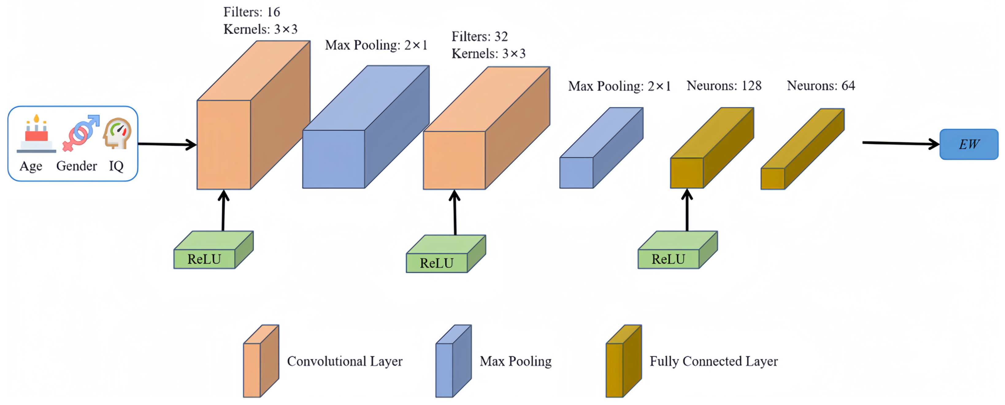
3.3. Multimodal Data Dusion to Build the Edges of the Graph

For constructing the edges of the graph, traditional methods often rely on random initialization or Euclidean distance [28], depending on the associations between the data in the original task. In this study, for the ASD automatic diagnosis task, we propose a method called edge-building network to determine the presence of edges between nodes and assign weights to these edges.

According to clinical reports, the probability of ASD diagnosis is significantly higher in males than in females, making gender one of the crucial factors. Additionally, clinical studies have highlighted distinct characteristics regarding the age of ASD diagnosis. A study by the Centers for Disease Control and Prevention in 2023 found that the prevalence of ASD among 8-year-old children is 2.76%, with approximately 1 in 36 children diagnosed with ASD. In China, ASD is typically diagnosed around the ages of 3 to 4, representing the primary period for diagnosis. ASD prevalence rates among 7- to 9-year-old children are 2.7% in Iceland, 1.2% in Denmark, and 1.8% in Tokyo, Japan. Therefore, age is another crucial factor to be considered. Lastly, research by Watanabe and Rees [29] indicates that compared to control groups associated with IQ and neurotransmitter frequency, the intelligence quotient scores of individuals with autism are predicted by the stability of their brain dynamics. IQ is selected as one of the significant factors for constructing the edges of the graph in this study. Hence, gender, age, and IQ serve as the second modality in this study, utilized for constructing the edges of the graph.

We curated and processed demographic information for each participant from the ABIDE dataset. Specifically, for gender data, males were represented as 1 and females as 2 in the original data. We standardized this representation, mapping gender values to [0, 1], where 0 represents males and 1 represents females. For age data, which originally ranged from 6 to 64, we standardized and rescaled it to fit within the range [0, 1]. Similarly, we processed IQ data, specifically the Full-Scale IQ (FIQ) of participants, which ranged from 41 to 148. We standardized and rescaled the FIQ values to also fit within the range [0, 1]. The gender, age, and IQ data were then vectorized and encoded to generate processed data, which served as the input to the edge-building network.

The edge-building network is a convolutional neural network designed specifically for ASD automatic diagnosis in this study. The network architecture is illustrated in Figure 3. Demographic information undergoes feature learning through the edge-building network, and the edge weights between two participants are calculated using cosine similarity. The purpose of this method is to fully explore and utilize the potential relationships and patterns within demographic information to enhance the diagnostic classification performance of the GCN for ASD.

As shown in Figure 3, the edge-building network consists of two convolutional layers, two pooling layers, and subsequent fully connected layers. Specifically, the first layer is a convolutional layer with 16 filters and a filter size of 3, allowing the model to capture local patterns within demographic data. This layer utilizes the ReLU activation function to introduce non-linearity and facilitate rapid gradient descent. Subsequently, the first pooling layer applies 2 × 1 max-pooling [30] operations to reduce feature dimensions while retaining the most important feature information. The second convolutional layer enhances the model’s learning capacity by further extracting complex feature patterns using 32 filters. Similarly, this layer employs the ReLU activation function [31]. The second pooling layer then applies 2 × 1 max-pooling again to further reduce feature dimensions and aggregate important information. Following the convolutional and pooling layers, the model integrates learned features through a fully connected layer containing 128 neurons. The ReLU activation function is used in this layer to increase the model’s expressive power. Finally, the output layer is designed as another fully connected layer with 64 units, directly outputting feature vectors for cosine similarity calculation. This layer does not use an activation function to facilitate the direct output of feature representations. This design allows us to compute the cosine similarity between individuals based on high-level features extracted by the CNN model, thereby assigning edge weights based on these similarities when constructing edges for the GCN.

By calculating the cosine similarity of demographic information between two participants, we can obtain the edge weight $E{W}_{uv}$ between two nodes as shown in (4):

$$E{W}_{uv}=\frac{UV}{‖U‖‖V‖},$$

(4)

Here, $U$ and $V$ represent the feature vectors of demographic information for two participants after undergoing feature learning with CNN. The value of cosine similarity [32] falls within the range of −1 to 1, where 1 indicates that the two vectors are identical, −1 indicates complete dissimilarity, and 0 denotes independence between the two vectors.

With this design, the edge-building network can effectively extract valuable features from demographic information and utilize these features to determine the edge weights for the GCN. This enables a more refined and accurate analysis of the diagnostic classification of ASD.

3.4. Improved Spectral Graph Convolutional Neural Network

This study is based on improvements to the spectral graph convolutional neural network. DropEdge is proposed, and residual connections are introduced to mitigate the issues of oversmoothing and neighborhood explosion in GCNs. Specifically, the concept of spectral graph convolution [33] exploits the fact that convolution is a multiplication in the Fourier domain. A graph Fourier transform is an operation defined by Laplace’s eigenfunction analog to the Euclidean domain. For a picture, the Laplace operator is actually a Laplace matrix $L$. Specifically, the Laplace matrix can then be expressed as:

$$L=D-A,$$

(5)

which is the degree matrix minus the adjacency matrix. By normalizing the Laplace matrix, we obtain:

$$L=I_N-D^{-\frac{1}{2}}A{D}^{-\frac{1}{2}},$$

(6)

The Laplace matrix, as a positive semidefinite matrix with real symmetry of $\mathsf{\Lambda }$, is capable of spectral decomposition, and further eigendecomposition yields:

$$L=U\mathsf{\Lambda }{U}^T,$$

(7)

where $U=\left(u_1,u_2,\dots ,u_n\right)$ is the eigenmatrix.

The Laplacian eigenvector is the basis of the Fourier transform, and performing a Fourier transform [34] on the graph is equivalent to representing the graph using a linear combination of the Laplacian matrix eigenvectors $U^T$. Therefore, for the features $x$ of the nodes in the graph, the traditional Fourier formula is transformed into a graph-based Fourier formula as follows:

$$f(x)={\displaystyle \int f(t)e^{-i2\pi xt}}dt={\displaystyle \sum _{n=1}^{N}f(n)u_t(n)}=U^{T}x,$$

(8)

According to the convolution theorem, the traditional convolution operation can be transformed into the convolution operation located on the graph as follows:

$$\begin{array}{l}\left(x\ast g\right)\left(t\right)=F^{-1}\left[F\left[x\left(t\right)\right]\odot F\left[g\left(t\right)\right]\right]\\ F^{-1}\left[F\left[x\left(t\right)\right]\odot F\left[g\left(t\right)\right]\right]=U\left(\left(U^{T}x\right)\odot \left(U^{T}g\right)\right)\end{array},$$

(9)

where $\odot$ represents the Hadamard product. We use a learnable convolution $g_{\theta }$ to denote $U^{T}g$. Then, the Hadamard product can be represented in the form of matrix multiplication, and the spectral graph convolution is represented in the following form.

$$U{g}_{\theta }{U}^{T}x,$$

(10)

To improve the computational efficiency and focus on the node neighborhood information and to execute the above computationally heavy spectral convolution, Defferrard et al. [35] proposed using Chebyshev polynomials [36] to approximate the convolution kernel.

$$g_{\theta }={\displaystyle \sum _{k=0}^{K-1}{\beta }_k{T}_k\left(\tilde{\mathsf{\Lambda }}\right)},$$

(11)

where $T_k\left(\cdot \right)$ is a Chebyshev polynomial of order $k$, ${\beta }_k$ is the corresponding coefficient (iteratively updated during training), and $\tilde{\mathsf{\Lambda }}=\frac{2\mathsf{\Lambda }}{{\lambda }_{\max }}-I_N$ is the rescaled eigenvalue diagonal matrix. We substitute (11) into (10) and substitute the matrix operation into the Chebyshev polynomial to obtain the convolution operation for a GCN layer.

$$y=\mathrm{G}\left({\displaystyle \sum _{k=0}^{K-1}{\beta }_k{T}_k\left(U\tilde{\mathsf{\Lambda }}{U}^T\right)x}\right),$$

(12)

where $\mathrm{G}$ is the activation function, and substituting (7) into the above formula, the final convolution operation is defined as:

$$y=\sigma \left({\displaystyle \sum _{k=0}^{K-1}{\beta }_k{T}_k\left(\tilde{L}\right)x}\right),$$

(13)

where $\tilde{L}=\frac{2L}{{\lambda }_{\max }}-I_N$. This eliminates the need for an eigendecomposition of the Laplace matrix [37] during the calculation. In the actual operation, the Chebyshev polynomial can be recursively used using the following property:

$$T_k\left(\tilde{L}\right)=2\tilde{L}{T}_k-1\left(\tilde{L}\right)-T_k-2\left(\tilde{L}\right),$$

(14)

In addition, $T_0\left(\tilde{L}\right)=I_N,T_1\left(\tilde{L}\right)=\tilde{L}$.

CNNs allow for the design and training of deep models, from which we derive the following relationship between layers of the GCN.

$$y^{\left(l+1\right)}=\mathrm{G}\left({\tilde{D}}^{-\frac{1}{2}}\tilde{A}{\tilde{D}}^{-\frac{1}{2}}{y}^{\left(l\right)}{W}^{\left(l\right)}\right),$$

(15)

where $y^{\left(l\right)}$ is the feature representation of layer $l$, $y^{\left(0\right)}=x$, $W^{\left(l\right)}$ is the learnable parameter of layer $l$, and $\tilde{D}$ is the degree matrix of the adjacency matrix $\tilde{A}$.

Deep GCNs are prone to neighborhood explosion and information loss issues. To address these, we introduce residual connections that combine the output of the first layer with the original input via a residual unit as the new output for the first layer. The output of the second layer is combined with the first layer’s output through a residual unit to serve as the new output for the second layer. Similarly, the output of the third layer is combined with the second layer’s output through a residual unit to form the new output for the third layer. Thus, the relationship between the layers of the GCN is shown in (16).

$$y^{\left(l+1\right)}=\mathrm{G}\left({\tilde{D}}^{-\frac{1}{2}}\tilde{A}{\tilde{D}}^{-\frac{1}{2}}{y}^{\left(l\right)}{W}^{\left(l\right)}\right)+y^{\left(l\right)},$$

(16)

The introduction of residual connections not only effectively mitigates the issues of gradient vanishing or explosion in deep networks and alleviates the neighborhood explosion problem in deep GCNs but also supports the construction of deeper network models. This enables the network to learn more complex and abstract feature representations, significantly improving model performance. Furthermore, residual connections, by directly adding the input to the output, allow for the direct flow of data, enabling the network to learn the residual mapping between the input and output.

During the training process of the GCN, we apply DropEdge once for every two layers of the population graph. In the training process, the first two layers do not perform any edge processing to ensure that the GCN can learn all features of the population graph. Before the input to the third layer, DropEdge is applied to the input population graph, meaning edges are randomly deleted from the population graph at a certain ratio. Similarly, DropEdge is applied before the input to the fifth layer. For the DropEdge operation, given an original graph $\mathrm{G}=(\mathrm{V},\mathrm{E})$, where $\mathrm{V}$ is the set of nodes and $\mathrm{E}$ is the set of edges, DropEdge generates a graph $\mathrm{G}=(\mathrm{V}, {\mathrm{E}}^{\prime })$ by randomly removing a certain proportion of edges from $\mathrm{E}$. For a layer in the GCN, after applying the DropEdge operation, the representation can be formulated as:

$$y^{\left(l+1\right)}=\mathrm{G}\left({\tilde{D}}^{-\frac{1}{2}}{\tilde{A}}^{\prime }{\tilde{D}}^{-\frac{1}{2}}{y}^{\left(l\right)}{W}^{\left(l\right)}\right)+y^{\left(l\right)},$$

(17)

where ${\tilde{A}}^{\prime }=A^{\prime }+I_N$ is the adjacency matrix $A^{\prime }$ after DropEdge processing added to the identity matrix $I_N$ (to include self-connections).

DropEdge, as a regularization technique designed for GCNs, can prevent overfitting and mitigate the oversmoothing issue. Its fundamental concept is derived from techniques similar to Dropout, where Dropout prevents model overfitting by randomly dropping some neurons in the neural network during the training process. Similarly, DropEdge randomly removes a portion of the edges in the graph during each training iteration. This approach can be seen as randomly sampling multiple subgraphs for training the GCN during the training process.

The improved spectral graph convolutional neural network designed in this study is shown in Figure 4. There are a total of six convolutional layers, each followed by a Leaky ReLU [38] activation function layer. The DropEdge regularization technique is applied after every two layers. $\otimes$ denotes the residual unit. Finally, we employ Dropout at the 2nd and 4th layers of the network to randomly remove a certain proportion of nodes, thereby increasing the diversity of subgraphs.

4. Results

4.1. Experiment Settings

In this study, we employed 10-fold cross-validation to train and test the ABIDE-I dataset, while adopting leave-one-out cross-validation to evaluate the ABIDE-II dataset. It is worth noting that leave-one-out cross-validation is particularly suitable for analyzing resting-state fMRI data due to its ability to maximize the use of limited sample sizes typical in brain imaging studies. It ensures every data point contributes to model training and validation, providing a comprehensive evaluation of the model’s performance. This approach is crucial in fields where data are scarce and highly variable, allowing for more accurate and detailed assessments essential for medical diagnostics, despite its higher computational demand compared to methods like 10-fold cross-validation. It is critical to conduct feature selection exclusively on the training dataset during each training phase, rather than on the entire dataset, to mitigate the issue of information leakage. This approach is vital for maintaining the credibility of model performance evaluations, an aspect often overlooked by many researchers. Neglecting this concern might result in inflated performance metrics on experimental datasets, whereas the model might underperform on new datasets, especially in scenarios requiring clinical application to new patients. Our methodology ensures consistent performance of the model on both new and experimental clinical data.

In this study, we utilized a third-order Chebyshev polynomial to approximate the convolutional kernel. We trained a GCN using the Adam optimizer for 300 epochs. The learning rate was set to 0.001, with a dropout rate of 0.2 and a DropEdge probability of 0.3. We implemented an early stopping mechanism with a patience parameter of 30 to prevent overfitting. The experiments were conducted on a Linux platform and executed via Python. Specifically, the experiment was run and debugged on a server equipped with an E5-2680 [email protected] GHz CPU and a GeForce RTX 4060 GPU using the Ubuntu 18.04 operating system. The model construction and experiments are implemented based on the PyTorch framework.

The evaluation metrics [39] include Accuracy, Precision, Recall, and Area Under the Curve (AUC), which are used to assess the model performance. Their equations are as follows:

$$\mathrm{Accuracy}=\frac{\mathrm{TP}+\mathrm{TN}}{\mathrm{TP}+\mathrm{TN}+\mathrm{FP}+\mathrm{FN}},$$

(18)

$$\mathrm{Precision}=\frac{\mathrm{TP}}{\mathrm{TP}+\mathrm{FP}},$$

(19)

$$\mathrm{Recall}=\frac{\mathrm{TP}}{\mathrm{TP}+\mathrm{FN}},$$

(20)

$\mathrm{TP}$ (True Positives) refers to the number of samples correctly identified as patients with ASD. $\mathrm{TN}$ (True Negatives) denotes the number of healthy control samples correctly identified as such. $\mathrm{FP}$ (False Positives) represents the number of samples from the healthy control group mistakenly identified as patients with ASD. $\mathrm{FN}$ (False Negatives) is the number of ASD patient samples incorrectly identified as belonging to the healthy control group.

4.2. Parametric Analysis

To ascertain which views contribute beneficially to the model’s performance in the multi-view scenario, we conducted individual experiments using a single-view approach for each different view. Subsequently, the best-performing view was selected for combination in multi-view experiments to determine the number and types of views. This study utilized five views: AAL, CC200, CC400, HO, and EZ. The results of the single-view experiments are presented in

Table 2. Results of single-view experiments.

View	Accuracy (%)	Precision (%)	Recall (%)	AUC
AAL	71.74	71.09	73.20	0.75
CC200	72.37	71.92	74.36	0.76
CC400	73.26	72.24	75.69	0.77
HO	70.42	69.78	72.10	0.74
EZ	69.53	70.11	71.35	0.73

.

From the results of the single-view experiments, it is evident that the CC400 view outperforms others, achieving the highest accuracy of 73.26% among all single-view experiments. Additionally, it demonstrates excellent performance in precision, recall, and AUC values. This suggests that the CC400 view plays a crucial and effective role in the diagnosis of ASD. Following closely, the CC200 view exhibits slightly lower accuracy, precision, recall, and AUC values compared to CC400 but still maintains high diagnostic performance. In contrast, the performance of the AAL, HO, and EZ views is slightly lower, with the EZ view showing the least favorable performance among them.

Next, we sorted the views based on their single-view accuracy and conducted experiments by combining different views into multi-view settings. The results of the multi-view experiments are depicted in Figure 5.

From the figure, it is evident that the performance of the model significantly improves as we move from single-view to multi-view combinations. Among single views, the CC400 view performs the best, with an accuracy of 73.26% and an AUC value of 0.77. When CC400 is combined with CC200, the accuracy increases to 76.45%, and the AUC value improves to 0.80. Further fusion with the AAL view results in the highest performance, with accuracy and AUC values reaching 78.31% and 0.84, respectively. However, when all five views are combined, there is a slight decrease in model performance, with accuracy dropping to 75.10% and AUC value to 0.79. This may suggest that adding more views leads to some redundancy in information among certain views.

4.3. Ablation Study

To evaluate the impact of the proposed multi-view attention fusion module, edge-building network, DropEdge, and residual connections on the model’s performance, we conducted ablation experiments. We conducted a total of five sets of experiments. Using GCN as the baseline model, the first set employed single-view fMRI data as input, with randomly initialized edges and training without DropEdge and residual connections. The second set used multi-view data with randomly initialized edges and without DropEdge and residual connections during training. The third set utilized multi-view data and reconstructed edge weights using the edge-building network, without using DropEdge and residual connections during training. The fourth set employed multi-view data and the edge-building network, utilizing DropEdge during training but without residual connections. The fifth set utilized multimodal data and the edge-building network, employing both DropEdge and residual connections during training. The experimental results are shown in

Table 3. Results of ablation experiments.

Method	Accuracy (%)	Precision (%)	Recall (%)	AUC
GCN	71.14	69.30	74.96	0.74
GCN + Fusion Module	73.62	73.72	77.09	0.77
GCN + Fusion Module + Edge-building network	76.38	76.33	79.82	0.80
GCN + Fusion Module + Edge-building network + DropEdge	77.25	77.51	80.56	0.82
MMGCN	78.31	78.18	81.73	0.84

.

From Table 3, it can be observed that the improved GCN with the multi-view and multimodal enhancements proposed in this paper exhibits the best performance. Specifically, as a baseline, the standalone GCN model provides preliminary performance metrics, including 71.14% accuracy, 69.30% precision, 74.96% recall, and an AUC value of 0.74. Upon incorporation of the multi-view fusion module into the GCN (GCN + Fusion Module), a significant improvement in all performance metrics is observed, indicating that the fusion of information from different brain region atlases can significantly enhance the model’s diagnostic capability. Furthermore, after integrating the edge-building network into the GCN fusion module (GCN + Fusion Module + Edge-building network), there is another increase in performance metrics, validating that leveraging demographic information between subjects to construct graph edges can effectively enhance the model’s classification accuracy. The introduction of the DropEdge technique (GCN + Fusion Module + Edge-building network + DropEdge) enhances the model’s resistance to overfitting, thereby further improving its performance. Finally, the addition of residual connections (Ours) yields the best results, indicating that residual connections help alleviate information loss in deep networks and facilitate the effective propagation of feature information.

4.4. Performance Evaluation

To ensure the comparability of results, we selected models with the same theme as baselines for comparison. They are DAE [40], ASD-DiagNet [41], and GCN [42], respectively. Additionally, to validate the advancement of the proposed MMGCN, we compared it with several state-of-the-art (SOTA) methods, namely MVS-GCN [43], Hi-GCN [44], and EV-GCN [45].

This study of DAE introduces an enhanced approach for analyzing fMRI data through a novel multi-kernel fuzzy clustering method combined with an auto-encoder for dimensionality reduction, significantly improving the clustering of brain networks for disorders like ASD.

ASD-DiagNet is a hybrid learning approach leveraging an autoencoder and a single-layer perceptron for classifying ASD from fMRI data. This method, distinct for its joint learning procedure and data augmentation strategy, outperforms state-of-the-art methods across multiple datasets, achieving significant accuracy improvements in ASD diagnosis.

This study of GCN introduces a novel framework for disease prediction, integrating graph convolutional networks with imaging and non-imaging data, showcasing enhanced prediction accuracy for Autism Spectrum Disorder and Alzheimer’s Disease.

MVS-GCN leverages a novel multi-view learning strategy within graph convolutional networks to better capture the complex relationships in brain connectivity data for disease diagnosis. This approach incorporates diverse data types and sources to construct a comprehensive graph-based representation, aiming to improve the understanding and identification of neurological disorders through advanced computational techniques.

Hi-GCN introduces a hierarchical graph convolutional network framework designed for brain network analysis. It uniquely integrates individual brain functional networks with population-level network correlations through a dual GCN model, aiming to improve the representation and diagnosis of brain disorders by leveraging both topological structure and node features within and across brain networks.

EV-GCN is a new framework enhancing disease prediction by dynamically learning graph edges in a graph convolutional network, integrating both imaging and non-imaging data for improved analysis.

This study utilized 10-fold cross-validation to conduct experiments on the aforementioned methods using the same dataset employed in this paper. The comparative results are shown in

Table 4. Results of comparative experiments on ABIDE-I.

Method	Accuracy (%)	Precision (%)	Recall (%)	AUC
DAE	69.26	63.84	76.41	0.70
ASD-DiagNet	70.41	70.47	71.55	0.72
GCN	71.14	69.30	74.96	0.74
MVS-GCN	70.08	66.23	71.02	0.70
Hi-GCN	74.36	66.89	72.67	0.79
EV-GCN	76.21	77.35	84.40	0.82
MMGCN	78.31	78.18	81.73	0.84

.

From Table 4, it can be observed that DAE achieved an accuracy of 69.26%, precision of 63.84%, recall of 76.41%, and an AUC of 0.70. This method shows strong recall, suggesting it effectively identifies positive cases but struggles with precision. ASD-DiagNet reported improvements with an accuracy of 70.41%, precision of 70.47%, recall of 71.55%, and an AUC of 0.72, indicating a more balanced performance between precision and recall. The GCN demonstrated a further increase in performance with an accuracy of 71.14%, precision of 69.30%, recall of 74.96%, and an AUC of 0.74, showcasing its strength in handling graph-based data. MVS-GCN showed a slight dip in certain metrics with an accuracy of 70.08%, precision of 66.23%, recall of 71.02%, and an AUC of 0.70, indicating challenges in multi-view integration. Hi-GCN significantly improved upon previous models with an accuracy of 74.36%, precision of 66.89%, recall of 72.67%, and an AUC of 0.79, highlighting the benefits of hierarchical modeling in graph networks. EV-GCN achieved impressive results with an accuracy of 76.21%, precision of 77.35%, recall of 84.40%, and an AUC of 0.82, demonstrating its effectiveness in dynamic edge adjustment for graph convolution.

Ours outperformed all mentioned methods, with the highest accuracy of 78.31%, precision of 78.18%, recall of 81.73%, and an AUC of 0.84, showcasing the proposed method’s superior ability to diagnose ASD accurately. In conclusion, while each compared method has its strengths, such as DAE’s recall capability, ASD-DiagNet’s balanced performance, GCN’s graph-based analysis, MVS-GCN’s multi-view integration, Hi-GCN’s hierarchical modeling, and EV-GCN’s dynamic edge adjustment, the MMGCN surpasses them by effectively combining these strengths. It addresses the limitations of each method by providing a comprehensive solution that leverages multi-view and multimodal data, incorporates dynamic edge adjustments, and mitigates the oversmoothing issue in GCNs, leading to the highest reported performance on the ABIDE-I dataset.

We further compare and analyze MMGCN with the other three SOTA methods. The ROC curves of these four methods are shown in Figure 6. In this study, the average ROC curve was used to evaluate the performance of the models. The curves in the figure represent the performance of different models in diagnosing ASD. Specifically, the curves for the MVS-GCN, Hi-GCN, EV-GCN, and MMGCN models show the true positive rate of these models at different false positive rates, respectively. The average ROC curves provide a visual comparison of the overall performance of the models by averaging the ROC curves for each fold of cross-validation. The larger the area of these curves, the greater the diagnostic ability of the model.

As seen in Figure 6, the MMGCN model has the highest AUC of 0.84, indicating the best performance in the ASD diagnosis task. Specifically, the ROC curves of all models show a rapid increase in the true positive rate when the false positive rate is close to 0, indicating better diagnostic performance at low false positive rates. However, as the false positive rate increases, the improvement in the true positive rate for each model gradually slows down. MMGCN outperforms the other models at all false positive rates, maintaining high diagnostic accuracy at different thresholds. In contrast, MVS-GCN performs the worst at high false positive rates, having the lowest true positive rate.

Between a false positive rate of 0.2 and 0.4, the gap between the models begins to widen significantly, with MMGCN performing most prominently at this stage, showing its advantage in balancing false positive and true positive rates. Overall, a detailed analysis of the ROC curves of the four models shows that MMGCN performs best in the ASD diagnostic task, followed by EV-GCN and Hi-GCN, with MVS-GCN performing the least effectively. This demonstrates that in terms of fusing multimodal data and improving the graph convolutional network, the design and implementation of MMGCN significantly enhance diagnostic performance.

To validate the robustness of the proposed MMGCN, we conducted experiments on the ABIDE-II dataset. We selected the same set of methods for comparison, namely DF-MCMPNA [46] and STCAL [47]. The DF-MCMPNA approach innovatively combines deep forest models with a multi-channel message passing and neighborhood aggregation mechanism to enhance brain network classification, focusing on capturing complex topological features effectively. The STCAL model employs a spatial–temporal co-attention learning mechanism to analyze resting-state fMRI data for mental disorder diagnosis, featuring a Guided Co-Attention module and a Sliding Cluster Attention module for enhanced pattern analysis and feature extraction. Due to the small size of the dataset, this study utilized leave-one-out cross-validation, which provides an unbiased estimate. The comparative experimental results are illustrated in Figure 7.

The analysis of Figure 7 reveals a detailed comparison of the proposed MMGCN against DF-MCMPNA and STCAL on the ABIDE-II dataset, focusing on accuracy, precision, recall, and AUC metrics. The MMGCN outperforms DF-MCMPNA and STCAL in all metrics, achieving the highest accuracy (75.62%), precision (74.88%), recall (79.07%), and AUC (0.79). This indicates a superior ability of the proposed method to diagnose ASD more accurately and reliably across these metrics.

The improved performance of the proposed MMGCN can be attributed to its innovative integration of multi-view and multimodal data through an enhanced graph convolutional network framework. This framework effectively leverages the complementary information present in different views and modalities, leading to a more robust and comprehensive analysis of brain networks. The use of advanced techniques such as DropEdge and residual connections further contributes to mitigating common issues like oversmoothing and information loss in deep GCNs, enhancing the model’s learning capability and generalization across different datasets. The superiority of the proposed method reflects its potential to provide more accurate and nuanced insights into ASD diagnosis, underscoring the importance of incorporating diverse data sources and sophisticated model architectures in medical diagnostics research.

4.5. Leave-One-Site-Out Cross-Validation

Since the ABIDE-I dataset is sourced from 17 different sites globally, it is crucial to validate the model’s cross-site capability. Leave-one-site-out cross-validation involves leaving out all data from one site for testing in each training and testing cycle, while data from the remaining sites are used for training. This means there are 17 training and testing cycles, each representing one of the 17 sites. The primary advantage of this method is its ability to assess the model’s generalization performance when faced with new site-specific data that was not included in the training phase. This is crucial for ensuring the robustness and transferability of the model, especially in applications where the model is expected to work across multiple different environments or conditions. In this study, GCN [42] and Hi-GCN [44] were selected as baselines to evaluate their accuracy using leave-one-site-out cross-validation. The results of leave-one-site-out cross-validation are presented in

Table 5. Results of leave-one-site-out cross-validation on ABIDE-I.

Site	Number	GCN	Hi-GCN	MMGCN
CALTECH	32	56.84	62.72	73.23
CMU	26	71.03	73.62	81.53
KKI	46	72.91	78.61	78.71
LEUVEN	54	64.69	70.57	75.80
MAX_MUN	45	47.83	53.52	70.71
NYU	160	72.17	80.98	80.07
OHSU	23	72.53	75.01	79.11
OLIN	33	67.14	69.60	82.04
PITT	51	73.56	79.08	74.87
SBL	27	57.05	62.62	81.71
SDSU	31	64.40	67.25	68.71
STANFORD	37	53.59	62.19	69.27
TRINITY	44	57.84	60.52	69.41
UCLA	90	68.49	71.27	73.76
UM	132	67.91	73.80	82.72
USM	67	70.49	79.00	68.99
YALE	51	66.15	75.01	77.63
Average	56	64.98	70.32	75.78

.

From the results in Table 5, we observe significant variations in accuracy across different sites in leave-one-site-out cross-validation. These findings reflect the heterogeneity among sites in terms of data collection procedures, participant demographics, and scanning protocols. Particularly, some sites exhibit accuracy below 70%, such as SDSU (68.71%), STANFORD (69.27%), TRINITY (69.41%), and USM (68.99%). These below-average performances may indicate that these sites possess unique characteristics or challenges, such as specific distributions of demographic features, variations in scanner settings, or differences in the severity distribution of ASD cases. These factors could potentially impact the model’s generalization capability and diagnostic accuracy.

Furthermore, the proposed MMGCN achieved the best performance for 14 out of the 17 sites, with an average accuracy of 75.78%, demonstrating significant superiority compared to the other two comparison methods. This outcome not only showcases the effectiveness of the proposed approach but also underscores the importance of adopting a multi-view and multi-modal fusion strategy when dealing with multi-site data. By leveraging brain imaging data and demographic information from different views effectively, the method proposed in this study is better equipped to capture the complex biological markers of ASD, thereby achieving more accurate automatic diagnosis in multi-site datasets.

5. Discussion

Observing the experimental results of the parametric analysis, we conclude that due to their broader coverage of brain regions and richer connectivity information, the CC400 and CC200 views exhibit superior performance in ASD diagnosis. This indicates the importance of considering the richness of brain region information and the diagnostic value of views when selecting brain atlas views for ASD diagnosis. Despite variations in the performance of individual views in ASD diagnosis, the functional connectivity information contained in different views is complementary. The AAL view may cover brain regions that are not fully characterized by the CC400 and CC200 views. Therefore, in practical applications, integrating multi-view information can leverage the advantages of each view to enhance the accuracy and robustness of ASD diagnosis. The poorer performance of the HO and EZ views relative to other views may be attributed to their lesser contribution in distinguishing between ASD and non-ASD groups or the sparsity of functional connectivity information in these views. Additionally, the inferior performance of the EZ view may be related to its specific brain region parcellation or coverage, highlighting the need to consider its applicability and limitations when using specific brain atlases.

The performance improvement of the multi-view fusion strategy demonstrates the complementarity between different views. Single views may only capture partial brain functional or structural features of ASD patients, while multi-view fusion can provide more comprehensive information, enhancing the model’s discriminative ability. Although multi-view fusion significantly improves performance initially, the phenomenon of performance decline after fusing all views suggests the need to balance the relationship between information gain and data redundancy during fusion. Too many views may introduce noise or irrelevant information, thereby reducing the model’s accuracy and generalization ability. Optimal performance occurs when the CC400, CC200, and AAL views are fused, indicating that selective view fusion is more effective than comprehensive fusion. Selective fusion can reduce redundant information while leveraging the complementarity of different views to improve model performance. Through multi-view fusion, the model demonstrates better generalization ability. This fusion strategy can effectively utilize information from different brain regions, improving the diagnostic accuracy of ASD, demonstrating the potential of this method in practical applications, and providing insights for future research.

Next, we further discuss the experimental results of the ablation study. The experimental results clearly demonstrate the importance of multi-view and multimodal information in improving ASD diagnostic performance. By integrating different types of data, the model is able to capture more comprehensive brain functional and structural features, thereby enhancing the accuracy of classification. The successful application of the DropEdge technique and residual connections further reveals effective strategies for combating overfitting and information loss when constructing deep learning models. DropEdge, by randomly removing parts of the graph edges, simulates different training subsets, and such regularization techniques effectively improve the model’s generalization ability. Meanwhile, residual connections ensure that even in deep model structures, information can still be effectively propagated, avoiding the problem of gradient disappearance, and allowing the model to learn deeper and more complex feature representations. While this paper primarily focuses on enhancing model performance, the application of multi-view fusion and multimodal information also provides potential avenues for understanding ASD biomarkers. By analyzing the contributions of different modules and techniques to performance improvement, further exploration of key brain regions and demographic features related to ASD can be pursued.

In performance evaluation, DAE demonstrates the potential of autoencoders in feature extraction but lacks the graph-based integration that is crucial for spatial data like fMRI, the accuracy and AUC of which the proposed MMGCN improves by 9.05% and 14%, respectively. ASD-DiagNet utilizes a hybrid learning approach that balances precision and recall better than DAE but still does not fully leverage the graph structure inherent in brain connectivity data. Our proposed MMGCN improves accuracy by 7.90% and AUC by 12%. GCN marks an improvement by incorporating graph-based analysis, yet it does not address the oversmoothing problem or fully utilize multimodal data, areas where the proposed method excels. Our method elevates the accuracy by 7.17% and the AUC by 10% compared to a traditional GCN. MVS-GCN attempts to integrate multi-view data but struggles with achieving consistency across different metrics, underscoring the proposed method’s more effective fusion strategy. Hi-GCN introduces hierarchical modeling to better capture the complex structure of brain networks, but it may not fully account for the multimodal nature of the data, unlike the proposed approach. EV-GCN shows a strong ability to dynamically adjust graph structures, significantly improving diagnosis accuracy. However, it might not fully exploit the multi-view data integration as effectively as the proposed method. Compared to the three SOTA methods, MVS-GCN, Hi-GCN, and EV-GCN, the MMGCN improves accuracy by 8.23%, 3.95%, and 2.10%, respectively.

The result of leave-one-site-out cross-validation not only demonstrates the efficiency and robustness of the MMGCN in multi-site ASD diagnosis tasks but also provides important guidance for future research. When designing deep learning models for diagnosing complex diseases, it is essential to consider the multi-view and multi-modal nature of the data, as well as the heterogeneity of cross-site data.

T-distributed Stochastic Neighbor Embedding (t-SNE) [48] is a nonlinear dimensionality reduction technique, particularly suitable for visualizing high-dimensional data in two- or three-dimensional space. This method aims to preserve the similarities between data points in high-dimensional space when representing them in a lower-dimensional space. As a result, similar data points are placed closer to each other in the reduced space, while dissimilar data points are positioned farther apart. Initially, t-SNE calculates the similarities between data points in the high-dimensional space. Then, it searches for a distribution of points in the lower-dimensional space that reflects these similarities to some extent. t-SNE uses Gaussian distributions to compute the similarities between each pair of data points in the high-dimensional space and converts these similarities into conditional probabilities. In the lower-dimensional space, t-SNE utilizes t-distributions to calculate the similarities between points, which helps address the “crowding problem”, where different categories of data points tend to be clustered together during the dimensionality reduction process. t-SNE seeks the optimal low-dimensional representation of the data by minimizing the Kullback–Leibler divergence between the similarities in the high-dimensional and low-dimensional spaces. This means that it attempts to make the distribution of points in the lower-dimensional space as close as possible to the distribution in the high-dimensional space.

The GCN is used to diagnose ASD, and t-SNE can be employed to visualize the distribution of graph nodes and edges constructed from fMRI and demographic information in a low-dimensional space. By mapping high-dimensional feature spaces into two-dimensional space, we can intuitively observe and analyze the relationships between data points, identifying potential patterns or clusters. Figure 8 illustrates the two-dimensional feature visualization of samples obtained from the original data and the MMGCN in this paper, with blue nodes representing ASD and red nodes representing HCs.

From Figure 8, it can be observed that the original data are distributed chaotically and disorderly in the two-dimensional space, with no clear boundaries. There is no apparent association between the ASD subgraph and the HC subgraph. This indicates the difficulty of the classification task and reflects the randomness of the data we used, demonstrating the robustness of the model. The samples obtained after using the MMGCN exhibit clear patterns in the two-dimensional space. Firstly, samples of the same category cluster together, indicating good intra-class cohesion of the results obtained by the MMGCN. Secondly, there is a certain symmetry between the ASD subgraph and the HC subgraph, reflecting the good inter-class discriminability of the results. Finally, samples of different types have relatively clear boundaries, indicating that our model has good classification performance.

The model’s superior performance is attributed to several key innovations. By integrating multi-view fMRI data through an attention fusion module and incorporating demographic data via an edge-building network, our approach captures a broader spectrum of diagnostic indicators, enhancing both sensitivity and specificity. This integration, combined with advanced regularization techniques such as DropEdge and residual connections, helps mitigate common deep learning challenges like oversmoothing and information loss, ensuring robust model performance across diverse datasets. The results of this study are a testament to the potential of deep learning in advancing the frontiers of medical diagnostics, particularly in the realm of neurodevelopmental disorders. The integration of diverse data sources and the employment of sophisticated model architectures have proven to be a fruitful avenue for enhancing the diagnostic capabilities of GCNs for ASD.

In conclusion, this study marks a significant step forward in the application of artificial intelligence for ASD diagnosis. The proposed method’s success underscores the importance of leveraging multi-view and multimodal data and paves the way for future research that could lead to more accurate, reliable, and accessible diagnostic solutions for neurodevelopmental disorders.

6. Conclusions

In this study, we introduced an enhanced graph convolutional neural network model that integrates fMRI and demographic data for the diagnosis of ASD. By employing a multi-view attention fusion module and an edge-building network, the method addresses the variability and complexity inherent in ASD diagnosis, enhancing the robustness and generalization capabilities of the diagnostic tool. Experimental results using two publicly available datasets demonstrate the superior performance of the MMGCN. Despite the promising outcomes, the study acknowledges certain limitations. The heterogeneous nature of ASD and the variability in data collection protocols across different sites present challenges in creating a universally applicable model. Furthermore, the reliance on demographic data for edge construction may introduce biases if the data are not representative of the broader population. The model’s performance may also be influenced by the quality and resolution of the fMRI data, as well as the selection of brain atlases for node construction. Future work could focus on refining the model to be more adaptable to diverse datasets and populations. This includes exploring methods to mitigate biases and improve the model’s generalization to understudied demographics. Additionally, incorporating more advanced techniques for handling the temporal dynamics of fMRI data could provide deeper insights into the neural underpinnings of ASD. Lastly, the integration of other modalities, such as genetic data or behavioral assessments, could lead to the development of a more comprehensive diagnostic tool for ASD.

References

1. Kenny, L.; Hattersley, C.; Molins, B.; Buckley, C.; Povey, C.; Pellicano, E. Which terms should be used to describe autism? Perspectives from the UK autism community. Autism 2015, 20, 442–462. [Google Scholar] [CrossRef] [PubMed]
2. Hirota, T.; King, B.H. Autism Spectrum Disorder. JAMA 2023, 329, 157–168. [Google Scholar] [CrossRef] [PubMed]
3. Wang, C.; Xiao, Z.; Wu, J. Functional connectivity-based classification of autism and control using SVM-RFECV on rs-fMRI data. Phys. Medica 2019, 65, 99–105. [Google Scholar] [CrossRef] [PubMed]
4. Xu, K.; Sun, Z.; Qiao, Z.; Chen, A. Diagnosing autism severity associated with physical fitness and gray matter volume in children with autism spectrum disorder: Explainable machine learning method. Complement. Ther. Clin. Pract. 2024, 54, 101825. [Google Scholar] [CrossRef] [PubMed]
5. Rathore, A.; Palande, S.; Anderson, J.S.; Zielinski, B.A.; Fletcher, P.T.; Wang, B. Autism Classification Using Topological Features and Deep Learning: A Cautionary Tale. Med. Image Comput. Comput. Assist. Interv. 2019, 11766, 736–744. [Google Scholar] [CrossRef]
6. Chen, J.; Liao, M.; Wang, G.; Chen, C. An intelligent multimodal framework for identifying children with autism spectrum disorder. Int. J. Appl. Math. Comput. Sci. 2020, 30, 435–448. [Google Scholar] [CrossRef]
7. Wang, M.; Zhang, D.; Huang, J.; Shen, D.; Liu, M. Low-Rank Representation for Multi-center Autism Spectrum Disorder Identification. Med. Image Comput. Comput. Assist. Interv. 2018, 11070, 647–654. [Google Scholar] [CrossRef] [PubMed]
8. Mostafa, S.; Tang, L.; Wu, F.-X. Diagnosis of Autism Spectrum Disorder Based on Eigenvalues of Brain Networks. IEEE Access 2019, 7, 128474–128486. [Google Scholar] [CrossRef]
9. Guo, X.; Wang, J.; Wang, X.; Liu, W.; Yu, H.; Xu, L.; Li, H.; Wu, J.; Dong, M.; Tan, W.; et al. Diagnosing autism spectrum disorder in children using conventional MRI and apparent diffusion coefficient based deep learning algorithms. Eur. Radiol. 2022, 32, 761–770. [Google Scholar] [CrossRef]
10. Epalle, T.M.; Song, Y.; Liu, Z.; Lu, H. Multi-atlas classification of autism spectrum disorder with hinge loss trained deep architectures: ABIDE I results. Appl. Soft Comput. 2021, 107, 107375. [Google Scholar] [CrossRef]
11. Ma, H.; Cao, Y.; Li, M.; Zhan, L.; Xie, Z.; Huang, L.; Gao, Y.; Jia, X. Abnormal amygdala functional connectivity and deep learning classification in multifrequency bands in autism spectrum disorder: A multisite functional magnetic resonance imaging study. Hum. Brain Mapp. 2023, 44, 1094–1104. [Google Scholar] [CrossRef]
12. Heinsfeld, A.S.; Franco, A.R.; Craddock, R.C.; Buchweitz, A.; Meneguzzi, F. Identification of autism spectrum disorder using deep learning and the ABIDE dataset. Neuroimage Clin. 2018, 17, 16–23. [Google Scholar] [CrossRef] [PubMed]
13. Lu, Z.; Wang, J.; Mao, R.; Lu, M.; Shi, J. Jointly Composite Feature Learning and Autism Spectrum Disorder Classification Using Deep Multi-Output Takagi-Sugeno-Kang Fuzzy Inference Systems. IEEE ACM Trans. Comput. Biol. Bioinform. 2023, 20, 476–488. [Google Scholar] [CrossRef] [PubMed]
14. Kashef, R. ECNN: Enhanced convolutional neural network for efficient diagnosis of autism spectrum disorder. Cogn. Syst. Res. 2022, 71, 41–49. [Google Scholar] [CrossRef]
15. Ahmed, M.R.; Zhang, Y.; Liu, Y.; Liao, H. Single Volume Image Generator and Deep Learning-Based ASD Classification. IEEE J. Biomed. Health Inf. 2020, 24, 3044–3054. [Google Scholar] [CrossRef] [PubMed]
16. Zhang, J.; Feng, F.; Han, T.; Gong, X.; Duan, F. Detection of Autism Spectrum Disorder using fMRI Functional Connectivity with Feature Selection and Deep Learning. Cogn. Comput. 2022, 15, 1106–1117. [Google Scholar] [CrossRef]
17. Wang, M.; Guo, J.; Wang, Y.; Yu, M.; Guo, J. Multimodal Autism Spectrum Disorder Diagnosis Method Based on DeepGCN. IEEE Trans. Neural Syst. Rehabil. Eng. 2023, 31, 3664–3674. [Google Scholar] [CrossRef]
18. Sarraf, A.; Khalili, S. An upper bound on the variance of scalar multilayer perceptrons for log-concave distributions. Neurocomputing 2022, 488, 540–546. [Google Scholar] [CrossRef]
19. Williams, C.M.; Peyre, H.; Toro, R.; Beggiato, A.; Ramus, F. Adjusting for allometric scaling in ABIDE I challenges subcortical volume differences in autism spectrum disorder. Hum. Brain Mapp. 2020, 41, 4610–4629. [Google Scholar] [CrossRef]
20. Di Martino, A.; O’Connor, D.; Chen, B.; Alaerts, K.; Anderson, J.S.; Assaf, M.; Balsters, J.H.; Baxter, L.; Beggiato, A.; Bernaerts, S.; et al. Enhancing studies of the connectome in autism using the autism brain imaging data exchange II. Sci. Data 2017, 4, 170010. [Google Scholar] [CrossRef]
21. Vincent, P.; Larochelle, H.; Lajoie, I.; Bengio, Y.; Manzagol, P.-A.; Bottou, L. Stacked denoising autoencoders: Learning useful representations in a deep network with a local denoising criterion. J. Mach. Learn. Res. 2010, 11, 3371–3408. [Google Scholar]
22. Messaritaki, E.; Foley, S.; Schiavi, S.; Magazzini, L.; Routley, B.; Jones, D.K.; Singh, K.D. Predicting MEG resting-state functional connectivity from microstructural information. Netw. Neurosci. 2021, 5, 477–504. [Google Scholar] [CrossRef] [PubMed]
23. Xu, H.; Deng, Y. Dependent Evidence Combination Based on Shearman Coefficient and Pearson Coefficient. IEEE Access 2018, 6, 11634–11640. [Google Scholar] [CrossRef]
24. van Aert, R.C.M. Meta-analyzing partial correlation coefficients using Fisher’s z transformation. Res. Synth. Methods 2023, 14, 768–773. [Google Scholar] [CrossRef] [PubMed]
25. Wang, Y.; Yao, H.; Zhao, S. Auto-encoder based dimensionality reduction. Neurocomputing 2016, 184, 232–242. [Google Scholar] [CrossRef]
26. Li, Z.; Hou, B.; Wu, Z.; Guo, Z.; Ren, B.; Guo, X.; Jiao, L. Complete Rotated Localization Loss Based on Super-Gaussian Distribution for Remote Sensing Images. IEEE Trans. Geosci. Remote Sens. 2023, 61, 5618614. [Google Scholar] [CrossRef]
27. Malinen, M.I.; Fränti, P. Clustering by analytic functions. Inf. Sci. 2012, 217, 31–38. [Google Scholar] [CrossRef]
28. Wang, M.; Ma, Z.; Wang, Y.; Liu, J.; Guo, J. A multi-view convolutional neural network method combining attention mechanism for diagnosing autism spectrum disorder. PLoS ONE 2023, 18, e0295621. [Google Scholar] [CrossRef] [PubMed]
29. Watanabe, T.; Rees, G. Brain network dynamics in high-functioning individuals with autism. Nat. Commun. 2017, 8, 16048. [Google Scholar] [CrossRef]
30. Mian, X.; Bingtao, Z.; Shiqiang, C.; Song, L. MCMP-Net: MLP combining max pooling network for sEMG gesture recognition. Biomed. Signal Process. Control 2024, 90, 105846. [Google Scholar] [CrossRef]
31. Xu, Y.; Zhang, H. Convergence of deep ReLU networks. Neurocomputing 2024, 571, 127174. [Google Scholar] [CrossRef]
32. Liu, Z.; Huang, H. Comment on “New cosine similarity and distance measures for Fermatean fuzzy sets and TOPSIS approach”. Knowl. Inf. Syst. 2023, 65, 5151–5157. [Google Scholar] [CrossRef]
33. Bai, J.; Ding, B.; Xiao, Z.; Jiao, L.; Chen, H.; Regan, A.C. Hyperspectral Image Classification Based on Deep Attention Graph Convolutional Network. IEEE Trans. Geosci. Remote Sens. 2022, 60, 3066485. [Google Scholar] [CrossRef]
34. Sandryhaila, A.; Moura, J.M.F. Discrete Signal Processing on Graphs. IEEE Trans. Signal Process. 2013, 61, 1644–1656. [Google Scholar] [CrossRef]
35. Defferrard, M.; Bresson, X.; Vandergheynst, P. Convolutional neural networks on graphs with fast localized spectral filtering. In Proceedings of the 30th Conference on Neural Information Processing Systems (NIPS 2016), Barcelona, Spain, 5–10 December 2016; Volume 29. [Google Scholar]
36. Ganji, R.M.; Jafari, H.; Baleanu, D. A new approach for solving multi variable orders differential equations with Mittag–Leffler kernel. Chaos Solitons Fractals 2020, 130, 109405. [Google Scholar] [CrossRef]
37. Tikhomirov, A.N. Limit Theorem for Spectra of Laplace Matrix of Random Graphs. Mathematics 2023, 11, 764. [Google Scholar] [CrossRef]
38. Nayef, B.H.; Abdullah, S.N.H.S.; Sulaiman, R.; Alyasseri, Z.A.A. Optimized leaky ReLU for handwritten Arabic character recognition using convolution neural networks. Multimed. Tools Appl. 2021, 81, 2065–2094. [Google Scholar] [CrossRef]
39. Canbek, G.; Taskaya Temizel, T.; Sagiroglu, S. BenchMetrics: A systematic benchmarking method for binary classification performance metrics. Neural Comput. Appl. 2021, 33, 14623–14650. [Google Scholar] [CrossRef]
40. Lu, H.; Liu, S.; Wei, H.; Tu, J. Multi-kernel fuzzy clustering based on auto-encoder for fMRI functional network. Expert. Syst. Appl. 2020, 159, 113513. [Google Scholar] [CrossRef]
41. Eslami, T.; Mirjalili, V.; Fong, A.; Laird, A.R.; Saeed, F. ASD-DiagNet: A Hybrid Learning Approach for Detection of Autism Spectrum Disorder Using fMRI Data. Front. Neuroinform. 2019, 13, 70. [Google Scholar] [CrossRef]
42. Parisot, S.; Ktena, S.I.; Ferrante, E.; Lee, M.; Guerrero, R.; Glocker, B.; Rueckert, D. Disease prediction using graph convolutional networks: Application to Autism Spectrum Disorder and Alzheimer’s disease. Med. Image Anal. 2018, 48, 117–130. [Google Scholar] [CrossRef] [PubMed]
43. Wen, G.; Cao, P.; Bao, H.; Yang, W.; Zheng, T.; Zaiane, O. MVS-GCN: A prior brain structure learning-guided multi-view graph convolution network for autism spectrum disorder diagnosis. Comput. Biol. Med. 2022, 142, 105239. [Google Scholar] [CrossRef] [PubMed]
44. Jiang, H.; Cao, P.; Xu, M.; Yang, J.; Zaiane, O. Hi-GCN: A hierarchical graph convolution network for graph embedding learning of brain network and brain disorders prediction. Comput. Biol. Med. 2020, 127, 104096. [Google Scholar] [CrossRef] [PubMed]
45. Huang, Y.; Chung, A.C.S. Disease prediction with edge-variational graph convolutional networks. Med. Image Anal. 2022, 77, 102375. [Google Scholar] [CrossRef] [PubMed]
46. Ji, J.; Li, J. Deep Forest with Multi-Channel Message Passing and Neighborhood Aggregation Mechanisms for Brain Network Classification. IEEE J. Biomed. Health Inf. 2022, 26, 5608–5618. [Google Scholar] [CrossRef] [PubMed]
47. Liu, R.; Huang, Z.A.; Hu, Y.; Zhu, Z.; Wong, K.C.; Tan, K.C. Spatial-Temporal Co-Attention Learning for Diagnosis of Mental Disorders from Resting-State fMRI Data. IEEE Trans. Neural Netw. Learn. Syst. 2023. Epub ahead of print. [Google Scholar] [CrossRef]
48. Ke, Q.; Zhang, J.; Wei, W.; Damasevicius, R.; Wozniak, M. Adaptive Independent Subspace Analysis of Brain Magnetic Resonance Imaging Data. IEEE Access 2019, 7, 12252–12261. [Google Scholar] [CrossRef]
Figure 1. The overall methodological framework.
Mathematics 12 01648 g001
Figure 2. Multi-view data fusion framework.
Mathematics 12 01648 g002
Figure 3. Edge-building network framework.
Mathematics 12 01648 g003
Figure 4. The improved spectral graph convolutional neural network framework.
Mathematics 12 01648 g004
Figure 5. Results of multi-view experiments.
Mathematics 12 01648 g005
Figure 6. ROC curves for different methods.
Mathematics 12 01648 g006
Figure 7. Results of comparative experiments on ABIDE-II.
Mathematics 12 01648 g007
Figure 8. Results of 2D feature visualization. (a) Original feature distribution; (b) post-classification feature distribution.
Mathematics 12 01648 g008